An efficient shape parametrisation by free-form deformation enhanced by active subspace for hull hydrodynamic ship design problems in open source environment

Abstract

In this contribution, we present the results of the application of a parameter space reduction methodology based on active subspaces property to the hull hydrodynamic design problem. In the framework of such typical naval architecture problem, several parametric deformations of an initial hull shape are considered to assess the influence of the shape parameters considered on the hull total drag. The hull resistance, which is the performance parameter associated with each parametric hull, is typically computed by means of numerical simulations of the hydrodynamic flow past the ship. Such problem is extremely relevant at the preliminary stages of the ship design, when several flow simulations are typically carried out by the engineers to establish a certain sensibility on the total drag dependence on the hull geometrical parameters considered and on other physical parameters. Given the high number of geometric and physical parameters involved –which might result in a high number of time consuming hydrodynamic simulations– assessing whether the parameters space can be reduced would lead to considerable computational cost reduction at the design stage. Thus, the main idea of this work is to employ the active subspaces to identify possible lower dimensional structures in the parameter space, or to verify the parameter distribution in the position of the control points. To this end, a fully automated procedure has been implemented to produce several small shape perturbations of an original hull CAD geometry which are then used to carry out high-fidelity flow simulations in different cruise conditions and collect data for the active subspaces analysis. To achieve full automation of the open source pipeline described, both the free form deformation methodology employed for the hull perturbations and the high fidelity solver based on unsteady potential flow theory, with fully nonlinear free surface treatment, are directly interfaced with CAD data structures and operate using IGES vendor-neutral file formats as input files. The computational cost of the fluid dynamic simulations is further reduced through the application of dynamic mode decomposition to reconstruct the final, steady state total drag value given only few initial snapshots of the simulation. The active subspaces analysis is here applied to the geometry of the DTMB-5415 naval combatant hull, which is a common benchmark in ship hydrodynamics simulations, within the SISSA mathLab applied mathematics lab. The contribution will discuss several details of the implementation of the tools developed, as well as the results of their application to the target engineering problem.

1 Introduction

Active subspaces (AS) has emerged as a useful parameter study technique in the last years (see [7]). It allows to identify a low dimensional structure in the parameter space of the scalar output function of interest. It uses a linear combination of all the parameters as new variable in order to reveal such lower dimensional behaviour of the output function. The aim of the present work is to investigate on the application of AS to reduce the number of parameters involved in the deformation of a particular hull geometry. Not only such investigation might result in a direct indication of a model reduction strategy for the problem at hand, but it can also illustrate how the AS algorithm can be applied to generic design problems to check whether a further reduction of dimensionality is possible.

To feed the AS algorithm, the relationship between the shape (input) parameters and the different fluid dynamic performance (output) parameters must be assessed. This has been done through a campaign of high-fidelity fluid dynamic simulations. In each of such simulations, the hull model has been morphed according to the deformation corresponding to the sample point in the parameters space.

As for the shape parametrization strategy, in the framework of reduced order modeling (ROM) we adopted a so-called general purpose shape morphing, that is a technique that does not depend on the particular shape to deform. As possible choices we mention free form deformation (FFD), inverse distance weighting (IDW) or radial basis functions (RBF) interpolation. All these methods basically involve the displacement of some control points in order to deform a domain. The displacements of these control points are what we identify as parameters. In this work we use the FFD since it allows global deformations of the geometry with only few parameters (see [22]).

The fluid dynamic solver used in this work is based on fully nonlinear potential flow model, implemented in the software WaveBEM ([15, 16]). Being directly interfaced with CAD data structures, the solver is able to import the deformed geometries, automatically generate the computational grids and carry out the simulation with no need for human interaction. The unsteady flow simulations were significantly accelerated through the use of dynamic mode decomposition (DMD) methodology. Since its introduction in the fluid mechanics community, DMD has emerged as a useful tool for analyzing the dynamics of nonlinear systems, by the approximation of the Koopman operator (see [21]). We will exploit the linear finite dimensional Koopman operator to reduce the computational cost of a single high-fidelity simulation. The DMD method allows to reconstruct the system dynamics through few snapshots describing the state of the system. With this approximation we can also infer on the future evolution of the system, allowing us to simulate only few seconds using the high-fidelity solver. We underline that both the pressure and velocity fields are reconstructed through the DMD.

The paper will briefly present all the aforementioned methodologies, and details of their application to the hull design problem considered. The results of the combined application of DMD and AS to the outputs of the fluid dynamic simulations will also be presented and discussed.

2 Estimation of the resistance of a hull advancing in calm water

In this section we introduce the problem of the estimation of the resistance of a ship advancing in calm water. The hull shape considered in this work is that of the DTMB 5415, which was conceived for the preliminary design of a US Navy Combatant ship and includes a sonar dome and a transom stern (see Figure 1). Given the abundance of experimental data available in the literature (among others, we cite [19]) has become a common benchmark for naval hydrodynamics simulation tools.

Figure 1: Reference domain $\Omega$, that is the DTMB 5415 hull.

We denote with $\Omega\subset\mathbb{R}^{3}$ the domain (see Figure 1) associated with our model hull. More specifically, $\Omega$ is our reference domain, and corresponds with the undeformed DTMB 5415 hull — the latter assumption is not fundamental for the remainder of the paper, but is convenient for practical reasons. We must here remark that the domain considered in the fluid dynamic simulations is in principle the volume of water $\Omega_{w}$ surrounding the hull. Further details about the fluid dynamic domain will be provided in the following sections.

We define the shape morphing $\mathcal{M}(\boldsymbol{x};\boldsymbol{\mu}):\mathbb{R}^{3}\to\mathbb{R}^{3}$ that maps the reference domain $\Omega$ into the deformed domain $\Omega(\boldsymbol{\mu})$, namely:

$$\Omega(\boldsymbol{\mu})=\mathcal{M}(\Omega;\boldsymbol{\mu}).$$

It is quite natural to infer that the flow field, and thus the result of the fluid dynamic simulations, will depend on the specific hull shape considered. In turn, such shape is associated to the parameters defining the morphing $\mathcal{M}$ — which will be extensively defined in the next sections. One of the main purposes of this contribution is then to investigate the effect of the morphing parameters on the total resistance, the main fluid dynamic performance parameter. We must here remark that one of the geometrical quantities having the most effect on the resistance is the immersed volume of a hull shape, as higher volumes will generate higher drag values. If designers only consider the absolute resistance value, they might then disregard hull shapes that have relatively good drag performances despite having higher immersed volume. This is of course undesired and could be avoided adopting different strategies. A first possibility is considering a resistance value which is nondimensionalized using a measure of the displaced volume. In alternative, the morphing parameters could be constrained so as to impose a fixed hull immersed volume. Unfortunately, the former solution poses some problem in the identification of the most suitable nondimensionalization strategy resulting in resistance output indices truly independent of the hull immersed volume. As for the latter possibility, it would lead to an undesired complication of the shape parametrization methodology. In this work the effect of immersed volume variations on the hull resistance is taken into account in a more natural fashion. In the fluid dynamic simulations, the rigid motions of the hull are also considered. In this way, once the ship displacement is imposed, the hull shape considered in the simulation reaches the equilibrium position under the action of gravity and hydrodynamic forces. When a shape morphing is characterized by a higher volume, the computed sink will reduce to obtain the same vertical component of the hydrodynamic force. This ensures that each shape is compared on a level ground.

By a practical standpoint, once a point in the parameter domain $\mathbb{D}$ is identified, the specific hull geometry is provided to the fluid dynamic solver, which carries out a flow simulation to come up with a resistance estimate. In this framework free form deformation has been employed for the generation of a very large number of hull geometries based on the DTMB 5415 naval combatant hull shape morphing. Each geometry generated has been used to set up a high-fidelity hydrodynamic simulation with the desired ship displacement and hull speed. Since the serial time dependent high-fidelity simulations are quite time consuming, taking approximatively 24 hours to reach a steady state solution, we adopted a reduction strategy based on dynamic mode decomposition (DMD) to cut the overall computational cost of each simulation to roughly 10 hours. The output resistances for all the configurations tested have been finally analyzed by means of active subspaces (AS) in order to verify if a further reduction in the parameter space is feasible, which could significantly speed up the work of designers.

In the next sections, we will provide a brief description of the unsteady fully nonlinear potential fluid dynamic model used to carry out the high-fidelity simulations. We refer the interested reader to [15, 17, 16] for further information on the fully nonlinear potential free surface model, on its application to complex hull geometries, and on the treatment of the hull rigid motions respectively. In addition, we will describe the free form deformation morphing methodology implemented, and describe the dynamic mode decomposition strategy used to cut the computational time of the simulations. Finally, the active subspaces used to analyze the resistance dependence on the morphing parameters will be presented.

3 Fully nonlinear potential model

In the simulations we are only considering the motion of a ship advancing at constant speed in calm water. For such reason we solve the problem in a global, translating reference frame $\widehat{XYZ}$, which is moving with the constant horizontal velocity of the boat $\boldsymbol{V}_{\infty}=(V_{\infty},0,0)$. Thus, the $X$ axis of the reference frame is aligned with $\boldsymbol{V}_{\infty}$, the $Z$ axis is directed vertically (positive upwards), while the $Y$ axis is directed laterally (positive port side).

As aforementioned, the domain $\Omega_{w}(t)$ in which we are interested in computing the fluid velocity and pressure is represented by the portion of water surrounding the ship hull. The time varying shape of such domain — and in particular that of its boundary with the air above — is one of the unknowns of the fluid dynamic problem. By convention, we place the origin of the vertical axis $Z$ in correspondence with the undisturbed free surface level, and we start each simulation at time $t=0$ from such undisturbed configuration. Thus, $\Omega_{w}(t=0)=\mathbb{R}^{3}_{Z-}\ \Omega$, where $\mathbb{R}^{3}_{Z-}$ indicates the lower half-space of $\mathbb{R}^{3}$, for which $Z\leq 0$.

If overturning waves are not observed (which is typically the case for low cruise velocities typical of a ship), the domain $\Omega_{w}(t)$ is simply connected. So under the assumptions of irrotational flow and non viscous fluid the velocity field $\boldsymbol{v}(\boldsymbol{X},t)$ admits a representation through a scalar potential function $\Phi(\boldsymbol{X},t)$, namely

$$\boldsymbol{v}={\boldsymbol{\nabla}}\Phi={\boldsymbol{\nabla}}\left(\boldsymbol{V}_{\infty}\cdot\boldsymbol{X}+\phi\right)\qquad\qquad\forall\ \boldsymbol{X}\in\Omega_{w}(t),$$ (1)

in which $\phi(\boldsymbol{X},t)$ is the perturbation potential. Under the present assumptions, the equations of motion simplify to the unsteady Bernoulli equation and to the Laplace equation for the perturbation potential:

$$\frac{\partial\phi}{\partial t}+\frac{1}{2}\left|{\boldsymbol{\nabla}}\phi+\boldsymbol{V}_{\infty}\right|^{2}+\frac{p-p_{a}}{\rho}-\boldsymbol{g}\cdot\boldsymbol{X}=C(t)\qquad \text{ in }\Omega_{w}(t),$$ (2a)

$$\Delta\phi=0 \text{ in }\Omega_{w}(t),$$ (2b)

where $C(t)$ is an arbitrary function of time, and $\boldsymbol{g}=(0,0,-g)$, is the gravity acceleration vector, directed along the $z$ axis. In the equation the constant water density $\rho$ and atmospheric reference pressure $p_{a}$ are also appearing. A noteworthy characteristic of the fluid dynamic problem at hand, is that the unknowns of such mathematical problem $\phi$ and $p$ are uncoupled. This means that the solution of the Poisson problem in Eq. (2b) can be obtained independently of the pressure field. Once such solution is obtained, the pressure can be obtained through a postprocessing step based on Bernoulli Eq. (2a). Thus, the Laplace equation is the governing equation of our model. Such equation is complemented by non penetration boundary conditions on the hull surface $\Gamma^{b}(t)$ and water basin bottom boundary $\Gamma^{bot}(t)$, and by homogeneous Neumann boundary conditions on the truncation boundaries $\Gamma^{far}(t)$ of the numerical domain. The bottom of the basin is located at a depth corresponding to 2 boat lenghts, while the truncation boundaries are located approximatively at a distance from the boat of 6 boat lengths in the longitudinal direction $X$ and of 2 boat lengths in the lateral direction $Y$). On the water free surface $\Gamma^{w}(t)$, we employ the kinematic and dynamic Semi-Lagrangian fully nonlinear boundary conditions, which respectively read

$$\frac{\delta\eta}{\delta t} = \frac{\partial\phi}{\partial z}+{\boldsymbol{\nabla}}\eta\cdot\left(\boldsymbol{w}-{\boldsymbol{\nabla}}\phi-\boldsymbol{V}_{\infty}\right)\qquad\text{ in }\Gamma^{w}(t),$$ (3)

$$\frac{\delta\phi}{\delta t} = -g\eta+\frac{1}{2}|{\boldsymbol{\nabla}}\phi|^{2}+{\boldsymbol{\nabla}}\phi\cdot\left(\boldsymbol{w}-{\boldsymbol{\nabla}}\phi-\boldsymbol{V}_{\infty}\right)\qquad\text{ in }\Gamma^{w}(t).$$ (4)

The former equation expresses the fact that a material point moving on the free surface will stay on the free surface — here assumed to be a single valued function $\eta(X,Y,t)$ of the horizontal coordinates $X$ and $Y$. The latter condition is derived from Bernoulli Eq. (2a), under the assumption of constant atmospheric pressure on the water surface. This peculiar form of the fully nonlinear boundary conditions was proposed in [4]. Eq. (3) allows for the computation of the vertical velocity of markers which move on the water free surface with a prescribed horizontal speed $(w_{X},w_{Y})$. Eq. (4) is used to obtain the velocity potential values in correspondence with such markers. The resulting vector $\boldsymbol{w}=(w_{X},w_{Y},\frac{\delta\eta}{\delta t})=\dot{\boldsymbol{X}}$ is the time derivative of the position of the free surface markers. In this work, such free surface markers are chosen as the free surface nodes of the computational grid. To avoid an undesirable mesh nodes drift along the water stream, the markers arbitrary horizontal velocity is set to 0 along the $X$ direction. The $Y$ component of the water nodes in contact with the ship — which is moved according with the computed linear and angular displacements — is chosen so as to keep such nodes on the hull surface. As for the remaining water nodes, the lateral velocity value is set to preserve mesh quality.

3.1 Three dimensional hull rigid motions

The equations governing the fluid dynamic problems are interfaced with the equations describing the dynamics of the hull — here supposed rigid. The evolution equation for the hull baricenter position $\boldsymbol{X}^{G}(t)$ is obtained via the linear momentum conservation equation, which in the case of our hydrodynamics simulation framework reads

$$m_{s}\ddot{\boldsymbol{X}}^{G}(t)=m_{s}\boldsymbol{g}+\boldsymbol{F}^{w}(t).$$ (5)

In Eq. (5), $m_{s}$ represents the mass of the ship, while the hydrodynamic force vector $\boldsymbol{F}^{w}(t)$ is obtained as the sum of the pressure and viscous forces on the hull.

The angular momentum conservation is instead written to obtain an evolution equation for the angular velocity ${\boldsymbol{\omega}}$ of the hull, namely

$$R(t)I^{G}R(t)^{T}\dot{{\boldsymbol{\omega}}}(t)+{\boldsymbol{\omega}}(t)\times R(t)I^{G}R(t)^{T}{\boldsymbol{\omega}}(t)=\boldsymbol{M}^{w}(t),$$ (6)

where the hydrodynamic moment vector $\boldsymbol{M}^{w}(t)$ is the sum of the moment about the ship center of gravity of the pressure and viscous forces on hull, propeller and appendages. At a closer look, a further unknown appears in Eq. (6). The rotation matrix $R(t)$ is in fact to be determined during the simulation. Such matrix allows for the conversion of points coordinates from the global reference frame $\widehat{XYZ}$ to the hull attached reference frame $\widehat{xyz}$ in which the hull geometry is described and the hull moment of inertia $I^{G}$ is computed, namely $\boldsymbol{X}(t)=R(t)\boldsymbol{x}+\boldsymbol{X}^{G}(t)$. To obtain a set of equations which govern the time evolution of $R(t)$, we resort to hull quaternions (again, we refer to [23] and [17] for further detail on quaternions and their application to hull dynamics respectively). For the present work purposes a quaternion is a particular type of four element vector, namely $\boldsymbol{q}(t)=\left[s,\boldsymbol{v}\right]=s+v_{X}(t)\boldsymbol{e}_{X}+v_{Y}(t)\boldsymbol{e}_{Y}+v_{Z}(t)\boldsymbol{e}_{Z}$. If the norm of a quaternion (defined as $||\boldsymbol{q}(t)||=\sqrt{s(t)^{2}+v_{X}(t)^{2}+v_{Y}(t)^{2}+v_{Z}(t)^{2}}$) has a unit value, the quaternion identifies a rotation matrix by means of the relation

$$R=\left[\begin{array}[]{c c c}1-2v_{Y}^{2}-2v_{Z}^{2}&2v_{X}v_{Y}-2sv_{Z}&2v_{X}v_{Z}+2sv_{Y}\\ 2v_{X}v_{Y}+2sv_{Z}&1-2v_{Y}^{2}-2v_{Z}^{2}&2v_{Y}v_{Z}-2sv_{X}\\ 2v_{X}v_{Z}-2sv_{Y}&2v_{Y}v_{Z}+2sv_{X}&1-2v_{Y}^{2}-2v_{Z}^{2}\end{array}\right],$$ (7)

in which to lighten the notation we omitted the time dependence of both $R(t)$ and the components of $\boldsymbol{q}(t)$. Thus, a unit quaternion is associated with the hull, and allows for the computation of the rotation matrix at all times. The equation describing the time evolution for the hull unit quaternion $\boldsymbol{q}(t)$ is

$$\dot{\boldsymbol{q}}(t)={\displaystyle{1\over 2}}{\boldsymbol{\omega}}_{q}(t)\boldsymbol{q}(t),$$ (8)

where ${\boldsymbol{\omega}}_{q}(t)=\left[0,{\boldsymbol{\omega}}(t)\right]$ is the quaternion associated with the angular velocity vector ${\boldsymbol{\omega}}(t)$, and the quaternion internal product is defined as

$$\boldsymbol{q}_{1}\boldsymbol{q}_{2}=\left[s_{1},\boldsymbol{v}_{1}\right]\left[s_{2},\boldsymbol{v}_{2}\right]=\left[s_{1}s_{2}-\boldsymbol{v}_{1}\cdot\boldsymbol{v}_{2}\,,\,s_{1}\boldsymbol{v}2+s_{2}\boldsymbol{v}1+\boldsymbol{v}_{1}\times\boldsymbol{v}_{2}\right].$$ (9)

As quaternions only have four entries, there only is one extra variable used to describe the three degrees of freedom of a three dimensional rotation. This is far less redundant than writing an evolution equation for each of the nine entries in a three dimensional rotation matrix. The residual redundant degree of freedom involved in the hull quaternion evolution is easily eliminated imposing a unit constraint on its norm, so as to ensure that the hull quaternion always represents a pure rotation.

4 Discretization and numerical solution

The boundary value problem described in the previous section is governed by the linear Laplace operator. Nonetheless, the presence of boundary conditions Eqs. (3) and (4) make the problem nonlinear. More sources of nonlinearity are given by continuous change of the domain shape over time and by the arbitrary shape of the ship hull. At each time instant, we will compute the values of the unknown potential and node displacement fields by solving a specific nonlinear problem resulting from the spatial and time discretization of the original boundary value problem. The spatial discretization of the Laplace problem is based upon a boundary integral formulation described in detail in [15] and [12]. The domain boundary is partitioned into quadrilateral cells, on which bi-linear shape functions are used to approximate the surface, the flow potential values, and the normal component of its surface gradient. The resulting iso-parametric Boundary Element Method (BEM, see [5]) consists in collocating a Boundary Integral Equation (BIE) in correspondence with each node of the numerical grid, and computing a numerical approximation the integrals appearing in such equation. The linear algebraic equations obtained from such spatial discretization step are combined with the Ordinary Differential Equations (ODE) derived from the finite element spatial discretization of the fully nonlinear free surface boundary conditions in Eqs. (3) and (4). The spatial discretization described is carried out making use of the deal.II open source library for C++ implementation of finite element discretizations (see [3, 2]). To enforce strong coupling between the fluid and structural problem, the aforementioned system of Differential Algebraic Equations (DAE) is complemented by the equations of the rigid hull dynamics. The fully coupled DAE system solution is time integrated by means of an arbitrary order and arbitrary time step implicit Backward Difference Formula (BDF) scheme implemented in the IDA package of the open source C++ library SUNDIALS described in [13]. The potential flow model described has been implemented in a stand alone C++ software, the main features of which are described in [15].

As for the output of the simulations considered in this work, at each time step of the simulation, the wave resistance is computed as

$$R^{w}=\int_{\Gamma^{b}}p\boldsymbol{n}\,d\Gamma\cdot\boldsymbol{e}_{X},$$ (10)

where $p$ is the pressure value obtained introducing the computed potential in Eq. (2a). The inviscid fluid dynamic model drag prediction is then corrected by adding a viscous drag contribution obtained by means of the ITTC-57 formula reported in [18]. A full assessment of the accuracy of the high-fidelity fluid structure interaction solver described is clearly beyond the scope of the present work. Yet, for all the Froude numbers tested the computed total drag difference with respect to the measurements reported by [19] is less then 6% (again, we refer the interested reader to [15, 17, 16] for more details). Given the fact that all the geometries tested are deformations of the present hull, it is reasonable to infer that for each simulation carried out the accuracy of the high-fidelity model prediction will be similar to that of the results presented.

No parallel version of the fluid dynamic solver has currently been developed. For such reason, the computational time of 24 hours for each simulation (accounting for approximatively 5000 cells) is not particularly competitive with respect to parallel RANS solvers. Yet, the extremely small size of the simulation outputs and the simplicity of the surface mesh required for the simulations make the present solver ideal for fully automated simulation campaigns based on shape parametrization. Moreover, the solver is complemented with a mesh module directly interfaced with CAD data structures based on the methodologies for surface mesh generation described in [8]. At the start of each simulation, such feature allows for fully automated mesh generation from each hull shape assigned in the form of a — possibly non water-tight — IGES geometry. This makes the fully nonlinear potential solver described a particularly useful tool when used in the framework of design pipelines which involve testing a high number of parametrised shapes. As we will see, not only human user interaction is not required to carry out several hundreds simulations; but in addition the extremely reduced dimension of the BEM solution files allows for very simple file storing and for a fast post processing phase.

5 Shape parametrization through free form deformation

In this section we will briefly describe how the free form deformation (FFD) shape morphing strategy has been used to produce a parametrised set of modified DTMB 5415 hulls to be used in the fluid dynamic simulations. FFD is a versatile parametrization technique used for shape optimization in a variety of fields such as aerospace engineering, structural mechanics, and biomedical engineering among others. For further insight on the original formulation of FFD we suggest to see [22], while for a recent work we suggest [20]. One of the main features of FFD, is that it does not directly manipulate the geometrical object at hand. Instead it deforms a lattice of points built around the object itself, manipulating the whole space in which the geometry is embedded. This lattice has the topology of a hypercube of dimension equal to the dimension of the geometry we want to morph (3D in this work). The lattice is deformed using a trivariate tensor-product of B-spline functions. This produces a continuous and smooth deformation of the geometry. Such methodology has been implemented into a stand alone Python package PyGeM [1], which has been used to obtain the morphed geometries considered in the present work.

Figure 2 displays a detail of the DTMB 5415 sonar dome, surrounded by the points composing the FFD lattice. FFD is devised to only deform objects which fall within the FFD lattice, so the picture indicates that in this work we are only modifying the shape of the DTMB 5415 sonar dome. The green lattice points in the picture are the ones that have been moved to produce the deformations of domain $\Omega$ used in this work.

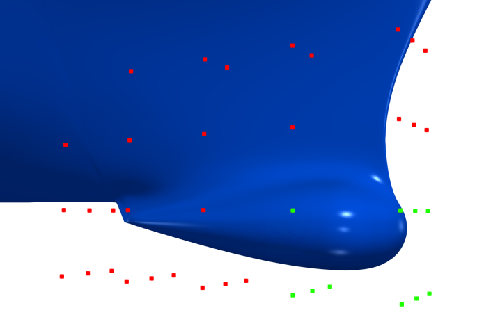
Figure 2: Control points of the FFD lattice around the bulbous bow. The points which are displaced to generate the hull deformations are indicated with the green color.

The FFD procedure can be in fact subdivided into three steps. First, the physical domain $\Omega$ is mapped to the reference domain $\widehat{\Omega}$ through a map $\psi$. Then, some control points (the green ones in the picture, in our case) $\boldsymbol{P}$ of the lattice are moved. Note that the displacement of such points are the parameters $\boldsymbol{\mu}$ that identify a particular deformed geometry. Once the lattice has been deformed, trivariate tensor-products of B-spline functions are used to compute the map $\widehat{T}$ that associates the original lattice to the deformed one. Finally, the back mapping from the deformed reference domain is applied to the deformed physical domain $\Omega(\boldsymbol{\mu})$ using the map $\psi^{-1}$. So it possible to express the FFD map $\mathcal{M}(\boldsymbol{x};\boldsymbol{\mu}):\Omega\subset\mathbb{R}^{3}\to\Omega(\boldsymbol{\mu})\subset\mathbb{R}^{3}$ by the composition of these three maps, i.e.

$$\mathcal{M}(\cdot\,;\boldsymbol{\mu})=(\psi^{-1}\circ\widehat{T}\circ\psi)(\cdot\,;\boldsymbol{\mu}).$$ (11)

In our case we have chosen $\boldsymbol{\mu}\in\mathbb{D}:=[-0.3,0.3]^{8}$, that results in a wide range of different bulbous bow configurations (see Figure 3 for an idea of different possible deformations). For sake of clarity we underline that the undeformed original domain is obtained setting all the geometrical parameters to 0. The main purpose of this work is to carry out a rather wide exploration of the shape parameter space, to assess the dependence of the output parameters on the shape morphing parameters. That is why the parameters bounds are chosen so as to be able to obtain somewhat significant — and yet physically meaningful — deformations of the bow bulb.

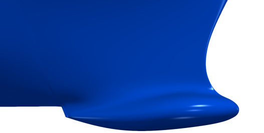
Figure 3: Two different examples of deformations.

6 System evolution reconstruction with dynamic mode decomposition

As mentioned, the unsteady and nonlinear fluid dynamic model adopted results in rather expensive simulations. Of course this could in principle reduced through full parallelization of the software developed which, however, has yet to be carried out. In this work, the computational cost of each simulation carried out has been reduced through the first application application of the dynamic mode decomposition (DMD) to our fully nonlinear potential solver output.

Dynamic mode decomposition (DMD) is a data-driven algorithm that provides a finite approximation of the infinite dimensional Koopman operator (see [14]). Proposed in [21] for fluid dynamics analysis, this technique has become popular in the last years mainly because (i) it allows to approximate nonlinear dynamics through low-rank structures that evolve in time and (ii) it relies only on the data, avoiding assumptions on the underlying system. We have implemented this algorithm, as well as many of its variants, in an open source Python package on GitHub, called PyDMD [10]. In this section we will introduce the DMD algorithm and we will discuss the fluid dynamic problem at hand as an example of its application. For an application of DMD to snapshots obtained from the solution of RANS equations see [9].

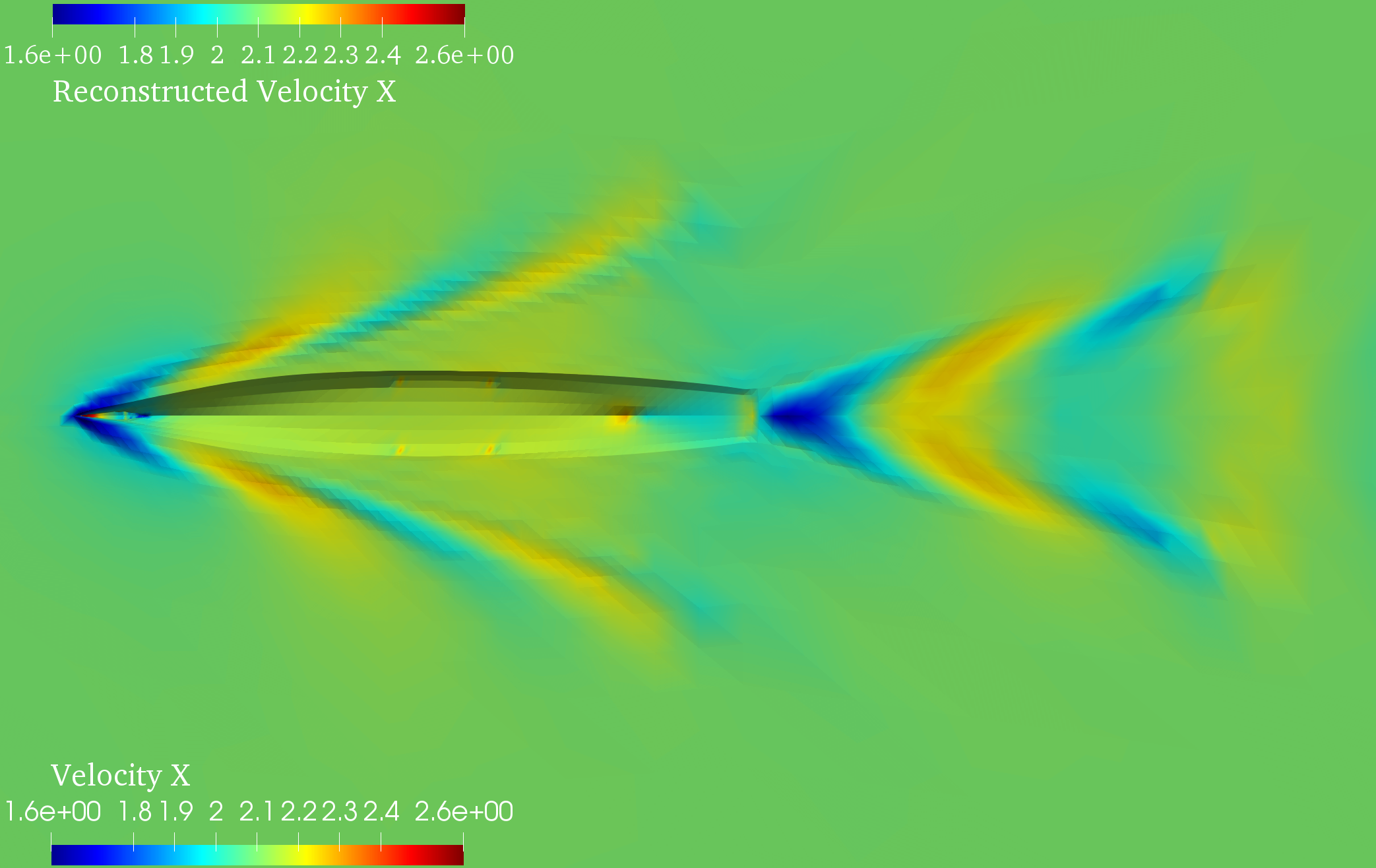
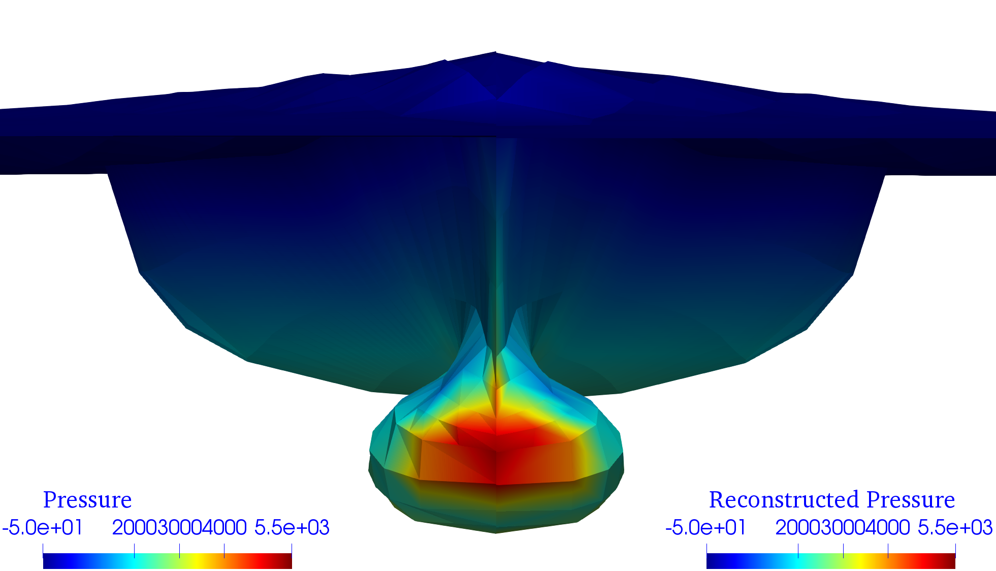
Figure 4: A comparison between the original output of the fluid dynamic simulations and the DMD reconstructed one. The top image represents a contour plot of water $X$ velocity around a morphing of the DTMB 5415 hull advancing at $\text{Fr}=0.28$ in calm water. The top half of the plot depicts the reconstructed fluid velocity, while the bottom half represents the one resulting from the high-fidelity computation. The bottom image is a front view of a contour plot of the pressure field on the hull and water surface. In this case, the left part of the plot refers to the high-fidelity solution, while the right half refers to the reconstructed pressure.

Let the variable $x_{k}$ represent the state of the evolving system at time $t_{k}=k\Delta t$. Basically, we want to find a linear finite dimensional Koopman operator $\mathbf{A}$ such that:

$$x_{k+1}=\mathbf{A}x_{k}$$ (12)

In order to build this operator, we collect a series of data vectors $\{x_{i}\}_{i=1}^{l}$, which we will refer to as snapshots from now on, and which represent the time-equispaced system states. We assume all the snapshots have the same dimension, that is $x_{k}\in\mathbb{R}^{n}$ for all $k=1,\dotsc,l$, and we assume the dimension $n$ of a snapshot is larger that the number of snapshots $l$, i.e. $n>l$. We arrange the snapshots in two matrices, $\mathbf{S}$ and $\mathbf{\dot{S}}$, as

$$\mathbf{S}=\begin{bmatrix}x_{1}^{1}&x_{2}^{1}&\cdots&x_{l-1}^{1}\\ x_{1}^{2}&x_{2}^{2}&\cdots&x_{l-1}^{2}\\ \vdots&\vdots&\ddots&\vdots\\ x_{1}^{n}&x_{2}^{n}&\cdots&x_{l-1}^{n}\end{bmatrix},\quad\quad\mathbf{\dot{S}}=\begin{bmatrix}x_{2}^{1}&x_{3}^{1}&\cdots&x_{l}^{1}\\ x_{2}^{2}&x_{3}^{2}&\cdots&x_{l}^{2}\\ \vdots&\vdots&\ddots&\vdots\\ x_{2}^{n}&x_{3}^{n}&\cdots&x_{l}^{n}\end{bmatrix}$$ (13)

in order to build the linear operator by minimizing $\|\mathbf{\dot{S}}-\mathbf{A}\mathbf{S}\|_{2}$. We underline that each column of $\mathbf{\dot{S}}$ contains the state vector at the next timestep of the one in the corresponding $\mathbf{S}$ column. Hence, the best-fit matrix $\mathbf{A}$ is given by:

$$\mathbf{A}=\mathbf{\dot{S}}\mathbf{S}^{\dagger}$$ (14)

where the symbol ^† denotes the Moore-Penrose pseudo-inverse. Since the snapshots usually have high dimension for complex systems, the matrix $\mathbf{A}$ becomes very large and it is difficult to manipulate. The DMD algorithm projects the data onto a low-rank subspace defined by the Proper Orthogonal Decomposition (POD) modes, then computes the low-dimensional operator $\tilde{\mathbf{A}}$. This operator is used to reconstruct the leading nonzero eigenvalues and eigenvectors of the full-dimensional operator $\mathbf{A}$ without ever explicitly computing $\mathbf{A}$. Using the truncated singular value decomposition of matrix $\mathbf{S}\approx\mathbf{U}_{r}\mathbf{\Sigma}_{r}\mathbf{V}^{*}_{r}$ with rank $r$, we can build the low-rank linear operator as:

$$\mathbf{\tilde{A}}=\mathbf{U}_{r}^{*}\mathbf{A}\mathbf{U}_{r}=\mathbf{U}_{r}^{*}\mathbf{\dot{S}}\mathbf{S}^{\dagger}\mathbf{U}_{r}=\mathbf{U}_{r}^{*}\mathbf{\dot{S}}\mathbf{V}_{r}\mathbf{\Sigma}_{r}^{-1}\mathbf{U}_{r}^{*}\mathbf{U}_{r}=\mathbf{U}_{r}^{*}\mathbf{\dot{S}}\mathbf{V}_{r}\mathbf{\Sigma}_{r}^{-1}.$$ (15)

We can now reconstruct the eigenvectors and eigenvalues of the matrix $\mathbf{A}$ using the eigendecomposition $\mathbf{\tilde{A}}\mathbf{W}=\mathbf{W}\mathbf{\Lambda}$. In detail (see [27]), the DMD modes $\mathbf{\Theta}$ can be computed by projecting the low-rank eigenvectors on the high-dimensional space $\mathbf{\Phi}=\mathbf{U}_{r}\mathbf{W}$ (projected modes) or computing the eigenvectors of $\mathbf{A}$ as $\mathbf{\Theta}=\mathbf{\dot{S}}\mathbf{V}_{r}\mathbf{\Sigma}_{r}^{-1}\mathbf{W}$ (exact modes). Moreover, the eigenvalues of $\mathbf{\tilde{A}}$ correspond to the nonzero eigenvalues of $\mathbf{A}$, and they contain the growth/decay rate and the frequencies of the corresponding modes. We recall Eq. (12) and underline that $\mathbf{A}=\mathbf{\Theta}\mathbf{\Lambda}\mathbf{\Theta^{\dagger}}$. The generic snapshot $x_{k+1}$ can be reconstructed by premultiplying the first snapshot $k$ times by the linear operator, such that $x_{k+1}=\mathbf{A}^{k}x_{1}=(\mathbf{\Theta}\mathbf{\Lambda}\mathbf{\Theta^{\dagger}}\dotsc\mathbf{\Theta}\mathbf{\Lambda}\mathbf{\Theta^{\dagger}})x_{1}$. Hence the state of the system can be approximated, for any time $t_{k+1}$ as:

$$x_{k+1}=\mathbf{\Theta}\mathbf{\Lambda}^{k}\mathbf{\Theta}^{\dagger}x_{1}$$ (16)

where the vector $\mathbf{\Theta}^{\dagger}x_{1}$ is usually called amplitudes.

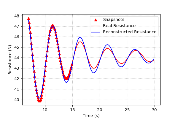
Figure 5: Comparison of high-fidelity (red continuous curve) and DMD reconstructed (blue continuous curve) total resistance time history. The triangular markers in the plot denote the times at which the snapshots for the DMD have been stored.

The application of DMD to the computational fluid dynamics simulations in this work is carried out collecting the snapshots within the temporal window $t=[7\ s,15\ s]$, with $\Delta t=0.1\ s$. As both the motion of the hull and of the free surface nodes are computed in the simulations, the DMD algorithm is educated using snapshot vectors which include the grid nodes coordinates, along with the flow velocity and pressure. The DMD algorithm has been used to compute a rather accurate approximation of the whole fluid dynamic problem solution up to $t=30\ s$, at the mere cost of a post processing phase requiring only few seconds. This led to a significant reduction of the computational cost, dropping the time required for each $30\ s$ simulation from $24\ h$ to $10\ h$.

Figure 4 compares the high-fidelity fluid dynamic solution at $t=30\ s$ with the one which has been reconstructed through the described DMD strategy. The figure includes both pressure and velocity field plots, which have been split in half to give a parallel view of both the high-fidelity and reconstructed field. Despite the DMD has been extrapolated from snapshots that are alder than $t=15\ s$, no difference between original and reconstructed flow and water elevation fields is appreciable in the contour plots. Figure 5 represents a comparison of time history of the hull resistance computed from the high-fidelity and DMD reconstructed hull pressure field. Again, the DMD approximated time history seems able to reconstruct with good approximation the the high-fidelity values. This is especially true for the last instants of the simulation, which are used to compute the final value of the total hull resistance, one of the output parameters considered in this work.

7 Parameter space verification and reduction by active subspaces

The active subspaces (AS) property has been brought to attention recently through the work of P. Constantine [7]. The AS property is a characteristic of the scalar function relating the scalar output to the parameters $\boldsymbol{\mu}$, and of a probability density function associated to such function. By a qualitative standpoint, AS is typically exploited to assess whether the parameter space allows for a significant — and of course useful — dimension reduction. By a quantitative standpoint, it can also be used to assess the sensitivity of the output with respect to each parameter considered. The main idea of AS is to operate in the parameters space, rescaling the inputs $\boldsymbol{\mu}$ and then rotating them with respect to the origin. In some cases (see [24, 26, 25]), such procedure reveals in lower dimension behavior of the output function $f(\boldsymbol{\mu})$ (the total resistance or the hull sink and trim, in our case). We underline that AS does not identify a subset of the inputs as important, instead it identifies a set of important directions in the space of all inputs. These directions (which are linear combinations of the input variables) are the ones along which the output function varies the most on average. When an active subspace is identified for the problem of interest, it is possible to perform different parameter studies.

Now we review how it is possible to find active subspaces. Let us assume $f:\mathbb{R}^{m}\rightarrow\mathbb{R}$ is a scalar function and $\rho:\mathbb{R}^{m}\rightarrow\mathbb{R}^{+}$ a probability density function, where $m$ is the dimension of the parameters. Since all the geometrical configurations can be drawn with equal probability, a uniform probability density will suffice in our case. In particular, we assume $f$ continuous and differentiable in the support of $\rho$, with continuous and square-integrable (with respect to the measure induced by $\rho$) derivatives. The active subspaces of the pair $(f,\rho)$ are the eigenspaces of the covariance matrix associated to the gradients $\nabla_{\boldsymbol{\mu}}f$. This matrix, denoted by $\boldsymbol{\Sigma}$, is the so-called uncentered covariance matrix of the gradients of $f$ (among others see [11] for a more deep understanding of these operators). Its elements are the average products of partial derivatives of $f$, that is:

$$\boldsymbol{\Sigma}=\mathbb{E}\,[\nabla_{\boldsymbol{\mu}}f\,\nabla_{\boldsymbol{\mu}}f^{T}]=\int_{\mathbb{D}}(\nabla_{\boldsymbol{\mu}}f)(\nabla_{\boldsymbol{\mu}}f)^{T}\rho\,d\boldsymbol{\mu},$$ (17)

where $\mathbb{E}[\cdot]$ is the expected value. We use a Monte Carlo method to approximate the eigenpairs of $\boldsymbol{\Sigma}$ as in [6]:

$$\boldsymbol{\Sigma}\approx\frac{1}{N_{\text{train}}^{\text{AS}}}\sum_{i=1}^{N_{\text{train}}^{\text{AS}}}\nabla_{\boldsymbol{\mu}}f_{i}\,\nabla_{\boldsymbol{\mu}}f^{T}_{i},$$ (18)

where we draw $N_{\text{train}}^{\text{AS}}$ independent samples $\boldsymbol{\mu}^{(i)}$ from the measure $\rho$ and where $\nabla_{\boldsymbol{\mu}}f_{i}=\nabla_{\boldsymbol{\mu}}f(\boldsymbol{\mu}^{(i)})$. The matrix $\boldsymbol{\Sigma}$ admits a real eigenvalue decomposition because it is symmetric positive semidefinite, so we have

$$\boldsymbol{\Sigma}=\mathbf{W}\mathbf{\Lambda}\mathbf{W}^{T},$$ (19)

where $\mathbf{W}$ contains the eigenvectors and is in $O(m)$, the orthogonal group, while $\mathbf{\Lambda}$ is the diagonal matrix of non-negative eigenvalues arranged in descending order.

The lower dimensional parameter subspace is formed by selecting the first $M<m$ eigenvectors. We underline that perturbations in the first set of coordinates change $f$, on average, more than perturbations in the second set of coordinates. We can discard the vectors corresponding to the low eigenvalues since they are in the nullspace of the covariance matrix. Doing so, we are able to construct an approximation of $f$. To be more clear, let us partition $\mathbf{\Lambda}$ and $\mathbf{W}$ as follows:

$$\mathbf{\Lambda}=\begin{bmatrix}\mathbf{\Lambda}_{1}&\\ &\mathbf{\Lambda}_{2}\end{bmatrix},\qquad\mathbf{W}=\left[\mathbf{W}_{1}\quad\mathbf{W}_{2}\right],$$

where $\mathbf{\Lambda}_{1}=\text{diag}(\lambda_{1},\dots,\lambda_{M})$, and $\mathbf{W}_{1}$ contains the first $M$ eigenvectors. The active subspace is the the range of $\mathbf{W}_{1}$. We call inactive subspace the range of the remaining eigenvectors in $\mathbf{W}_{2}$. The linear combinations of the input parameters with weights from the important eigenvectors are the active variables. By projecting the full parameter space onto the active subspace we can approximate the behaviour of $f$. In particular we have the following formulas for the active variable $\boldsymbol{\mu}_{M}$ and the inactive variable $\boldsymbol{\eta}$:

$$\boldsymbol{\mu}_{M}=\mathbf{W}_{1}^{T}\boldsymbol{\mu}\in\mathbb{R}^{M},\qquad\boldsymbol{\eta}=\mathbf{W}_{2}^{T}\boldsymbol{\mu}\in\mathbb{R}^{m-M}.$$ (20)

Using Eq. (20) and the fact that $\mathbf{W}\in O(m)$ we can express any point in the parameter space $\boldsymbol{\mu}\in\mathbb{R}^{m}$ in terms of $\boldsymbol{\mu}_{M}$ and $\boldsymbol{\eta}$ as follows:

$$\boldsymbol{\mu}=\mathbf{W}\mathbf{W}^{T}\boldsymbol{\mu}=\mathbf{W}_{1}\mathbf{W}_{1}^{T}\boldsymbol{\mu}+\mathbf{W}_{2}\mathbf{W}_{2}^{T}\boldsymbol{\mu}=\mathbf{W}_{1}\boldsymbol{\mu}_{M}+\mathbf{W}_{2}\boldsymbol{\eta}.$$

So it is possible to rewrite $f$ as

$$f(\boldsymbol{\mu})=f(\mathbf{W}_{1}\boldsymbol{\mu}_{M}+\mathbf{W}_{2}\boldsymbol{\eta}),$$

and, using only the active variables, we can construct a surrogate quantity of interest $g$

$$f(\boldsymbol{\mu})\approx g(\mathbf{W}_{1}^{T}\boldsymbol{\mu})=g(\boldsymbol{\mu}_{M}).$$

In our pipeline, the surrogate quantity of interest $g$ will be obtained by a response surface method.

8 Numerical Results

In this section we present the numerical results obtained by applying all the methodologies presented above to the DTMB 5415 model hull. The FFD morphing methodology illustrated has been used to generate 130 different deformations of the original hull. The parametrised shapes correspond to uniform sampling points in the parameter space box $\mathbb{D}=[-0.3,0.3]^{8}$. Each IGES geometry produced has been then used as the input of a high fidelity simulation in which the hull has been set to advance in calm water at a constant speed corresponding to $\text{Fr}=0.28$. Each high fidelity computation has been carried out to simulate $15\ s$ of the flow past the hull after it has been impulsively started from rest. Between the 7th and 15th second of the high-fidelity simulations, the solver saved the full flow field at sampling intervals $\Delta t=0.1\ s$. Such flow field snapshots have been used to feed the DMD algorithm implemented, and complete the fluid dynamic simulations until convergence to the regime solution was reached at $t=30\ s$. The reconstructed flow fields have been finally used to evaluate the hull total resistance and the hydrodynamic trim position, which are the output performance parameters considered in this work. The dataset composed by the output of the simulations has been divided in a train dataset (75% of the outputs) used to train the AS algorithm and a test dataset (25% of the outputs) used to validate the methodology.

Figure 6 depicts the eigenvalues estimates of the matrix $\boldsymbol{\Sigma}$ (black dots and line) and also displays the bootstrap intervals (corresponding to the grey area surrounding the eigenvalues lines). In the figure, the left plot is referred to the total resistance, while the right one is displays the hydrodynamic trim angle.

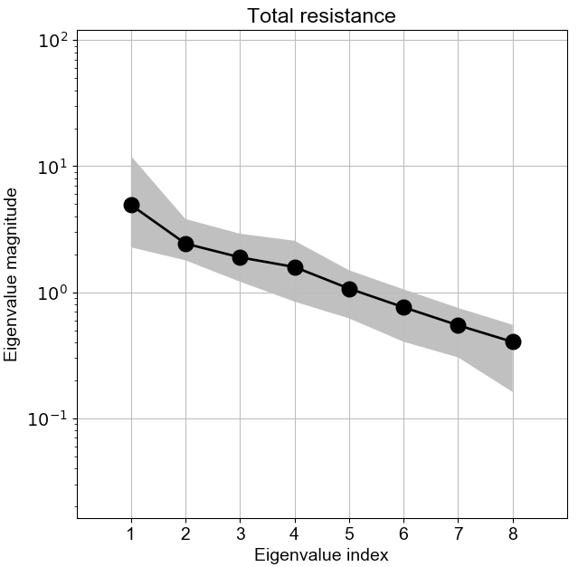
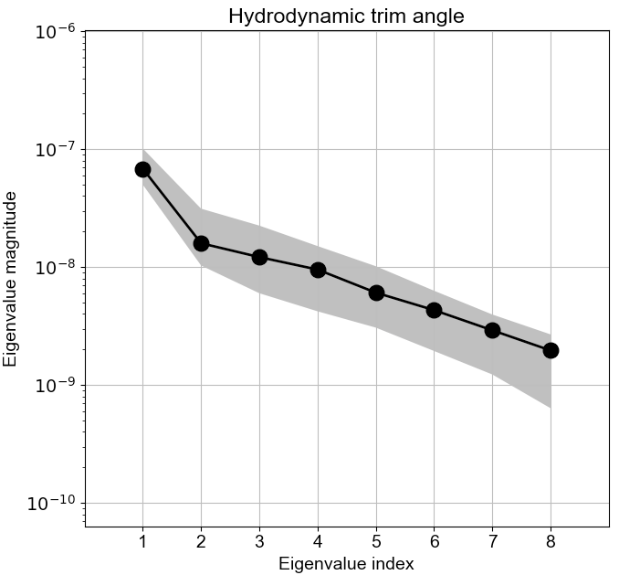
Figure 6: Eigenvalues estimates of the matrix $\boldsymbol{\Sigma}$ for the total resistance (on the left) and the hydrodynamic trim angle (on the right). The black dots in the plot indicate the eigenvalues, which the grey area is defined by the bootstrap intervals.

The plots indicate that a factor of at least 10 exists between the highest and lowest $\boldsymbol{\Sigma}$ eigenvalues. Such difference is clearly more pronounced when the hydrodynamic trim is the output considered. Yet, the plots also show that the eigenvalues magnitude is rather evenly distributed across the range they span. More precisely, the absence of a major gap between the higher module eigenvalues and the lower module ones, is suggesting that the active subspace is most revealing a clear cut low dimensional behaviour of the target functions with respect to the active variables, as is the case for different applications [24, 26]. Yet, especially in the case of the hydrodynamic trim angle output, the first eigenvalue module is considerably higher than that of the remaining ones. That is why, for the hydrodynamic trim it was possible to compute a bivariate surface response using the first two active variables, obtained as linear combinations of the original parameters with coefficients obtained by the eigenvectors corresponding to the two highest module eigenvalues. Figure 7 shows the quartic surface that best approximates the training dataset in the sense of least squares, along with the points in the test dataset (which are indicated by the dots). Each point represents the value of the target function $f(\boldsymbol{\mu})$ against the active variables $\boldsymbol{\mu}_{M}=\boldsymbol{W}_{1}^{T}\boldsymbol{\mu}\in\mathbb{R}^{2}$. As can be appreciated, the points corresponding to the true output are not distributed randomly in the space, but tend to be somewhat clustered around the surface. This is particularly true when the output parameter considered is the hydrodynamic trim angle (right plot) for which, as we have seen, the $\boldsymbol{\Sigma}$ eigenvalues corresponding to the first active variable was significantly higher then the remaining ones. Thus, whenever the gap between the leading $\boldsymbol{\Sigma}$ eigenvalues allows for it, the AS algorithm is able to successfully identify a set active variables upon which the output is — with reasonable approximation — exclusively depending.

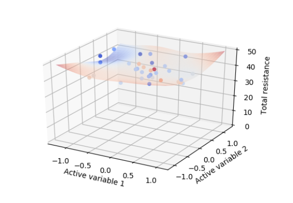
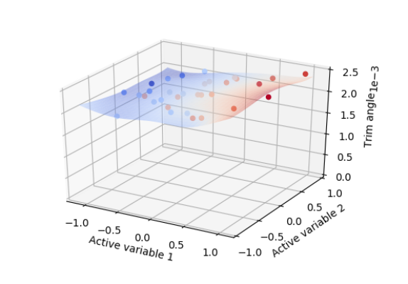
Figure 7: Comparison between the quartic surface response obtained with two active variables and the true output for the test dataset, indicated by the dots. The left plot refers to the total resistance output, while the right one to the hydrodynamic trim angle.

To provide a more quantitative assessment of how much such approximation is in fact reasonable, and depends on the gap existing between the first $\boldsymbol{\Sigma}$ eigenvalues and the following ones, we computed the average error as the average, among 10 different eigenvalues estimates, of the root mean square error divided by the maximum range of variation of the target function. As expected, the accuracy of the two dimensional surface response predictions for the hull total resistance is rather low, and only a 20% average error is obtained, that is about $1.8$ Newton. The average error obtained for the hydrodynamic trim angle output is approximatively 11%, that corresponds to an absolute rmse of $8\cdot 10^{-5}$, confirming that such output can be better represented through AS. Thus, for all those applications for which 10% can be considered an acceptable error — as might be the case for early design stages — AS provides a recipe to reduce the parameter space from 8 to 2 variables. In addition, the error analysis provides a further confirmation of the fact that once the eigenvalue analysis is carried out, the detection of a possible cliff in the eigenvalue curve (see Figure 6) is a measure of how well AS will perform. So, since the computational cost of the post processing operations required for the AS algorithm proposed is marginal with respect to that of the high-fidelity simulations, it should be always worth checking if AS could be used to obtain a significant drop in the parameter space dimension.

9 Conclusions and further developments

This work presented an application to naval hydrodynamics simulations of the active subspaces algorithm. Such algorithm can lead to a significant reduction of the parameter space dimension. The test case considered consisted in the flow past several parametrised modifications of the shape of a DTMB 5415 model hull. Such modified shapes were obtained by means of the free form deformation involving 8 parameters, and used for fully nonlinear potential flow simulations. The computational cost of the whole simulation campaign has been significantly reduced through the application of dynamic mode decomposition strategy to speedup the convergence of the unsteady simulation to the finial regime solution. The contribution describes the whole pipeline composed of shape parametrization, hydrodynamic simulations, and data post processing, all based on in house developed software.

The results obtained confirm that AS can be conveniently used to reduce the parameter space dimension when a significant gap is detected between the highest and lowest eigenvalues of the uncentered covariance matrix of the output gradients with respect to the input parameters. Yet, in the present case the hull total resistance (one of the two outputs considered) did not present such feature, resulting in a diminished effect of the AS parameter dimension reduction. As for the hydrodynamic trim angle, AS is able to provide more accurate two dimensional approximation of the output dependence on the eight shape parameters considered. The reduced computational cost of the post processing steps required for the AS analysis suggests that it can be used in any contest to check whether a reduction of the parametric space dimension is convenient.

Future work will focus on several areas to improve physical and mathematical aspects of the algorithms presented. Further developments of the whole pipeline will be implemented to better integrate its different parts and automate the simulation campaign and post processing processes.

References

- [1] PyGeM: Python Geometrical Morphing. Available at: https://github.com/mathLab/PyGeM.
- [2] W. Bangerth, D. Davydov, T. Heister, L. Heltai, G. Kanschat, M. Kronbichler, M. Maier, B. Turcksin, and D. Wells. The deal.II library, Version 8.4. Journal of Numerical Mathematics, 24(3):135–141, 2016.
- [3] W. Bangerth, R. Hartmann, and G. Kanschat. deal.II — A General Purpose Object Oriented Finite Element Library. ACM Transactions on Mathematical Software, 33(4):24/1–24/27, 2007.
- [4] R. F. Beck. Time-domain computations for floating bodies. Applied Ocean Research, 16:267–282, 1994.
- [5] C. A. Brebbia. The Boundary Element Method for Engineers. Pentech Press, 1978.
- [6] P. Constantine and D. Gleich. Computing active subspaces with Monte Carlo. arXiv preprint arXiv:1408.0545, 2015.
- [7] P. G. Constantine. Active subspaces: Emerging ideas for dimension reduction in parameter studies, volume 2. SIAM, Philadelphia, 2015.
- [8] F. Dassi, A. Mola, and H. Si. Curvature-adapted remeshing of cad surfaces. Procedia Engineering, 82:253–265, 2014.
- [9] N. Demo, M. Tezzele, G. Gustin, G. Lavini, and G. Rozza. Shape optimization by means of proper orthogonal decomposition and dynamic mode decomposition. Submitted; arXiv preprint arXiv:1803.07368, 2018.
- [10] N. Demo, M. Tezzele, and G. Rozza. PyDMD: Python Dynamic Mode Decomposition. The Journal of Open Source Software, 3(22):530, 2018.
- [11] J. L. Devore. Probability and Statistics for Engineering and the Sciences. Cengage Learning, 2015.
- [12] N. Giuliani, A. Mola, L. Heltai, and L. Formaggia. FEM SUPG stabilisation of mixed isoparametric BEMs: application to linearised free surface flows. Engineering Analysis with Boundary Elements, 8–22:59, 2015.
- [13] A. C. Hindmarsh, P. N. Brown, K. E. Grant, S. L. Lee, R. Serban, D. E. Shumaker, and C. S. Woodward. Sundials: Suite of nonlinear and differential/algebraic equation solvers. ACM Transactions on Mathematical Software (TOMS), 31(3):363–396, 2005.
- [14] B. O. Koopman. Hamiltonian systems and transformation in hilbert space. Proceedings of the National Academy of Sciences, 17(5):315–318, 1931.
- [15] A. Mola, L. Heltai, and A. DeSimone. A stable and adaptive semi-lagrangian potential model for unsteady and nonlinear ship-wave interactions. Engineering Analysis with Boundary Elements, 128–143:37, 2013.
- [16] A. Mola, L. Heltai, and A. DeSimone. Wet and Dry Transom Stern Treatment for Unsteady and Nonlinear Potential Flow Model for Naval Hydrodynamics Simulations. Journal of Ship Research, 61(1):1–14, 2017.
- [17] A. Mola, L. Heltai, A. DeSimone, et al. Ship Sinkage and Trim Predictions Based on a CAD Interfaced Fully Nonlinear Potential Model. In The 26th International Ocean and Polar Engineering Conference, volume 3, pages 511–518. International Society of Offshore and Polar Engineers, 2016.
- [18] A. Morrall. 1957 ITTC Model-ship Correlation Line Values of Frictional Resistance Coefficient. Ship report. National Physical Laboratory, Ship Division, 1970.
- [19] A. Olivieri, F. Pistani, A. Avanzini, F. Stern, and R. Penna. Towing tank experiments of resistance, sinkage and trim, boundary layer, wake, and free surface flow around a naval combatant insean 2340 model. Technical report, DTIC Document, 2001.
- [20] F. Salmoiraghi, A. Scardigli, and H. T. G. Rozza. Free Form Deformation, mesh morphing and reduced order methods: enablers for efficient aerodynamic shape optimization. Submitted; arXiv preprint arXiv:1803.04688, 2018.
- [21] P. J. Schmid. Dynamic mode decomposition of numerical and experimental data. Journal of fluid mechanics, 656:5–28, 2010.
- [22] T. Sederberg and S. Parry. Free-Form Deformation of solid geometric models. In Proceedings of SIGGRAPH - Special Interest Group on GRAPHics and Interactive Techniques, pages 151–159. SIGGRAPH, 1986.
- [23] K. Shoemake. Animating rotation with quaternion curves. In ACM Computer Graphics (Proc. SIGGRAPH), pages 245–254, 1985.
- [24] M. Tezzele, F. Ballarin, and G. Rozza. Combined parameter and model reduction of cardiovascular problems by means of active subspaces and POD-Galerkin methods. Submitted; arXiv preprint arXiv:1711.10884, 2017.
- [25] M. Tezzele, N. Demo, M. Gadalla, A. Mola, and G. Rozza. Model order reduction by means of active subspaces and dynamic mode decomposition for parametric hull shape design hydrodynamics. arXiv preprint arXiv:1803.07377, 2018.
- [26] M. Tezzele, F. Salmoiraghi, A. Mola, and G. Rozza. Dimension reduction in heterogeneous parametric spaces with application to naval engineering shape design problems. Submitted; arXiv preprint arXiv:1709.03298, 2017.
- [27] J. Tu, C. Rowley, D. Luchtenburg, S. Brunton, and N. Kutz. On dynamic mode decomposition: Theory and applications. Journal of Computational Dynamics, 1(2):391–421, 2014.