Pushing back the limits: detailed properties of dwarf galaxies in a $\Lambda$CDM universe

We present the results of a set of high resolution chemo-dynamical simulations of dwarf galaxies in a $\Lambda$CDM cosmology. Out of an original $(3.4\,\rm{Mpc}/h)^{3}$ cosmological box, a sample of 27 systems are re-simulated from z=70 to z=0 using a zoom-in technique. Gas and stellar properties are confronted to the observations in the greatest details: in addition to the galaxy global properties, we investigated the model galaxy velocity dispersion profiles, half-light radii, star formation histories, stellar metallicity distributions, and [Mg/Fe] abundance ratios. The formation and sustainability of the metallicity gradients and kinematically distinct stellar populations are also tackled. We show how the properties of six Local Group dwarf galaxies, NGC 6622, Andromeda II, Sculptor, Sextans, Ursa Minor and Draco are reproduced, and how they pertain to three main galaxy build-up modes. Our results indicate that the interaction with a massive central galaxy could be needed for a handful of Local Group dwarf spheroidal galaxies only, the vast majority of the systems and their variety of star formation histories arising naturally from a $\Lambda$CDM framework. We find that models fitting well the local Group dwarf galaxies are embedded in dark haloes of mass between $5\times 10^{8}$ to a few $10^{9}\,\rm{M_{\odot}}$, without any missing satellite problem. We confirm the failure of the abundance matching approach at the mass scale of dwarf galaxies. Some of the observed faint however gas-rich galaxies with residual star formation, such as Leo T and Leo P, remain challenging. They point out the need of a better understanding of the UV-background heating.

1 Introduction

Dwarf galaxies are the least luminous galactic systems with the largest dark-to-stellar mass ratio in the Universe. They are very sensitive to any perturbation, such as stellar feedback (radiative and thermal), environmental processes (gravitational interactions, ram pressure stripping), and heating by the cosmic UV-background. As such they constitute unique laboratories with which to infer the physics leading to the formation and evolution of galaxies. Last but not least, in the hierarchical $\Lambda$CDM paradigm, dwarf galaxies are the most numerous as well as first galaxies to be formed, playing a key role in the re-ionization of our Universe (Choudhury et al., 2008; Salvadori et al., 2014; Wise et al., 2014; Robertson et al., 2015; Bouwens et al., 2015; Atek et al., 2015).

The first generation of dark matter only (DMO) $\Lambda$CDM cosmological simulations conclude serious tensions between their results and the observations (see Bullock & Boylan-Kolchin (2017) for a recent review) : over-prediction of small mass systems around the Milky Way, the missing satellite problem (Klypin et al., 1999; Moore et al., 1999) and the too big to fail problem (Boylan-Kolchin et al., 2011, 2012). These DMO simulations also predicted the dark haloes to follow a universal cuspy profile (Navarro et al., 1996, 1997). while the observations seemed to favour cored ones (Moore, 1994). More recently Pawlowski et al. (2012); Pawlowski & Kroupa (2013); Ibata et al. (2013) have advocated a correlation in phase-space between both the Milky Way and the Andromeda satellites as if they were all located within a rotationally-supported disc. If definitively confirmed, such a configuration would be at odds with the $\Lambda$CDM predictions in which satellites are expected to be isotropically distributed.

On the one hand, these tensions have been a strong motivation for exploring alternative cosmologies that could directly impact the formation and evolution of dwarf galaxies (see for example Spergel & Steinhardt, 2000; Lovell et al., 2012; Rocha et al., 2013; Vogelsberger et al., 2014). On the other hand, they have led to studies revealing the strong impact of the baryonic physics on the faintest galaxies (Zolotov et al., 2012; Brooks & Zolotov, 2014). While the treatment of baryons in $\Lambda$CDM simulations remains challenging (Revaz et al., 2016b), significant improvements have recently been achieved to address the above issues.

High resolution hydro-dynamical simulations of the Local Group such as APOSTLE (Sawala et al., 2016) or Latte (Wetzel et al., 2016) demonstrated that the ram pressure and tidal stripping of the haloes orbiting their host galaxy, together with the reduction of their mass due to the UV-background heating and stellar feedback, strongly reduces the amplitude of the faint tail of the luminosity function. This potentially solves the missing satellite and too big to fail problems. While its reality is still debated (Pineda et al., 2017), the core-cusp problem may be solved by a very bursty star formation history induced by a strong feedback, transforming the central cusp into a large density core (Pontzen & Governato, 2014). This theoretical prediction has been reproduced in some cosmological hydro-dynamical simulations (Oñorbe et al., 2015; Chan et al., 2015; Fitts et al., 2017).

We are now at a stage where simulations are mature enough to allow detailed investigations of the properties of the systems arising from a $\Lambda$CDM universe at the level offered by present day observations. This last decade has seen a wealth of studies focused on the reproduction of the mean or integrated physical quantities of dwarfs such as their central velocity dispersion, mean metallicity, total luminosity, gas mass, and half light radius (Valcke et al., 2008; Revaz et al., 2009; Sawala et al., 2010; Schroyen et al., 2011; Revaz & Jablonka, 2012; Cloet-Osselaer et al., 2012; Sawala et al., 2012; Cloet-Osselaer et al., 2014; Sawala et al., 2016; Wetzel et al., 2016; Fitts et al., 2017; Macciò et al., 2017). Following the semi-analytical cosmological models (e.g. Salvadori et al., 2008), more and more hydrodynamical simulations include some stellar abundance patterns in their calculations (e.g. Escala et al., 2018; Hirai et al., 2017). To definitely validate any theoretical framework, we not only need to confront the model predictions to the mean galaxy properties via their scaling relations but also to go one step further and consider their structure, that is, the galaxy stellar velocity dispersion profiles, stellar metallicity distributions, stellar abundance ratios as well as more subtle properties such as their metallicity gradients or kinematically distinct stellar populations.

To do so, we can take advantage of a plethora of accurate observations in the Local Group dwarf galaxies. In addition to the standard morphological, gas and luminosity measurements (McConnachie, 2012), we have access to line-of-sight velocities revealing the galaxy stellar dynamics (ex. Walker et al., 2009a; Battaglia et al., 2008; Fabrizio et al., 2011, 2016). Deep colour magnitude diagrams allow to infer the galaxy star formation histories (Dolphin, 2002; de Boer et al., 2012a, b; Weisz et al., 2014a; de Boer et al., 2014; Weisz et al., 2014b; Santana et al., 2016; Kordopatis et al., 2016; Bettinelli et al., 2018). High resolution spectroscopic observations of individual stars allow us to determine accurate stellar abundances providing strong constraints on the galaxy chemical evolution (Shetrone et al., 2001, 2003; Fulbright et al., 2004; Sadakane et al., 2004; Koch et al., 2008; Aoki et al., 2009; Cohen & Huang, 2009; Frebel et al., 2010; Norris et al., 2010; Cohen & Huang, 2010; Tafelmeyer et al., 2010; Letarte et al., 2010; Kirby et al., 2010; Venn et al., 2012; Lemasle et al., 2012; Starkenburg et al., 2013; Jablonka et al., 2015; Tsujimoto et al., 2015).

Stellar population gradients, in other words a variation of the population properties with galacto-centric distances, provide constraints on the interplay between dynamics and chemical evolution (Harbeck et al., 2001; Tolstoy et al., 2004; Koch et al., 2006; Battaglia et al., 2006; Faria et al., 2007; Gullieuszik et al., 2009; Kirby et al., 2011; Battaglia et al., 2011; Vargas et al., 2014; Ho et al., 2015; Lardo et al., 2016; Spencer et al., 2017; Suda et al., 2017; Okamoto et al., 2017).

In the present study, we follow the formation and evolution of dwarf galaxies in a $\Lambda$CDM cosmological context, confronting the above observational constraints and the model predictions. This work leverages our previous and preparatory work on simulations of galaxies either in isolation (Revaz et al., 2009; Revaz & Jablonka, 2012; Revaz et al., 2016a), or interacting with a Milky-Way-like host, through tidal or ram pressure stripping (Nichols et al., 2014, 2015). While the present simulations are fully cosmological, they do not include a massive galaxy. Nevertheless the environmental impact on galaxy evolution is taken into account. Indeed, the model dwarfs experience accretion and merger events. They are also affected by the strong ionizing UV-background radiation, which has been identified as being capable of evaporating most of the gas in dwarf galaxies (Efstathiou, 1992; Quinn et al., 1996; Bullock et al., 2000; Noh & McQuinn, 2014) and forms a natural constraint to the period of reionization (Susa & Umemura, 2004; Ricotti & Gnedin, 2005; Okamoto et al., 2010; Shen et al., 2014).

This paper is organized as follows: In Section 2 we briefly describe our code, GEAR, its recent improvements and the settings of our cosmological zoom-in simulations. The results are presented in Section 3. They include the multi-phase structure of the gas (Section 3.2), the global properties of the dwarf galaxies (Section 3.3), and their star formation histories (Section 3.4), as well as the line of sight stellar velocity dispersion profiles, the stellar metallicity distribution function and the [Mg/Fe] abundance ratios (Section 3.5). The formation of the age and metallicity gradients are discussed in Section 3.6 and the origin of the kinematically distinct stellar populations in Section 3.7. We summarize our main results in Section 4.

2 Methods

All simulations presented in this work have been run with the chemo-dynamical Tree/SPH code GEAR, developed by Revaz & Jablonka (2012) and Revaz et al. (2016a). We summarize below its main features, which are presented in detail in the above references. GEAR is fully parallel based on Gadget-2 (Springel, 2005). It includes gas cooling, star formation, chemical evolution, and Type Ia and II supernova yields (Kobayashi et al., 2000; Tsujimoto et al., 1995) and thermal blastwave-like feedback (Stinson et al., 2006), for which 10% of the SNe explosion energy, taken as $10^{51}$ erg, is released in the interstellar medium ($\epsilon=0.1)$. GEAR follows the pressure-entropy SPH formulation of Hopkins (2013) and operates with individual and adaptive time steps as described in Durier & Dalla Vecchia (2012). In the following, the initial mass function (IMF) of each model stellar particle is sampled with the random discrete scheme (RIMFS) of Revaz et al. (2016a), i.e., a stochastic approach that reproduces well the discretization of the IMF. We employ the Smooth Metallicity Scheme that permits chemical mixing between stellar particles (Okamoto et al., 2005; Tornatore et al., 2007; Wiersma et al., 2009) and matches the observed low level of chemical scatter at very low metallicity in galactic haloes. The V-band luminosities are derived following the stellar population synthesis model of Vazdekis et al. (1996) computed for the revised Kroupa (2001) IMF used in our model.

The simulations of galaxies in isolation of GEAR have successfully reproduced the main observable properties of dSphs (Revaz & Jablonka, 2012), including their stellar metallicity distribution function and chemical abundance trends. We recently conducted an extensive study of the early pollution of the galaxy interstellar medium (ISM) and of the resulting dispersion in chemical abundance ratios, [$\alpha$/Fe], at low metallicity (Revaz et al., 2016a). GEAR has also been tested in the context of the Assembling Galaxies Of Resolved Anatomy (AGORA) project (Kim et al., 2016) where it demonstrated its ability to simulate Milky Way-like galaxies. The next section describes some of the recent improvements implemented in GEAR.

2.1 Cooling, UV-background heating and self-shielding

The radiative cooling of the gas has been updated with the Grackle cooling library (Smith et al., 2017) adopted by the AGORA project (Kim et al., 2014, 2016). We used the equilibrium cooling mode of the library (metals are assumed to be in ionization equilibrium) in which cooling rates have been pre-computed by the Cloudy photo-ionization code (Ferland et al., 2013). Cooling rates are tabulated as a function of the gas density, temperature and metallicity. They contain the contribution of the primordial cooling as well as metal line cooling determined for solar abundances. The latter contribution is scaled to the metallicity of the gas. The heating resulting from the presence of a redshift-dependent uniform UV-background radiation (Haardt & Madau, 2012) is also taken into account.

At high densities, the gas may no longer be considered as optically thin and hydrogen becomes self-shielded against the ionizing UV-background radiation. The critical density at which hydrogen becomes self-shielded is model dependent. It is sensitive to the method used (ray tracing, moment-based), the photo-ionization rates as well as to the exact spectrum of the ionizing photons considered and the adopted hydrogen cross section. At some level, it may also depend on the fitting formula used. Values ranging from $n_{\rm{H}}=10^{-3}$ to $n_{\rm{H}}=6\times 10^{-2}\,\rm{atom/cm^{3}}$ have been derived through different types of radiative transfer models (see for example Tajiri & Umemura, 1998; Aubert & Teyssier, 2010; Yajima et al., 2011; Rahmati et al., 2013). In the present work, we simulated the shielding multiplying the UV-heating by an Heaviside function centred on the density threshold $n_{\rm{H}}=0.007$, following Aubert & Teyssier (2010).

2.2 Star formation

The high resolution of our simulations leads us to deal with gas at densities higher than $1\,\rm{atom/cm^{3}}$ which reaches temperatures lower than $100\,\rm{K}$. These low temperatures result from the combined effect of the hydrogen self-shielding against the ionizing UV-background radiation (Tajiri & Umemura, 1998; Aubert & Teyssier, 2010; Yajima et al., 2011) and a very short cooling time. In such conditions, the Jeans length of the gas becomes very small, possibly smaller than the model spatial resolution and is no longer resolved. Consequently, the noise inherent to the model discretization may generate perturbations, leading to a spurious fragmentation of the gas (Truelove et al., 1997; Bate & Burkert, 1997; Owen & Villumsen, 1997). A classical solution to avoid this spurious fragmentation is to include an additional non-thermal pressure term in the equation of state of the gas, which ensures that the Jeans length is comparable to the resolution of the system (Robertson & Kravtsov, 2008; Schaye & Dalla Vecchia, 2008). This additional pressure can be interpreted as the non-thermal pressure due to the ISM turbulence, which is unresolved. Here, we have used the following pressure floor, which is a modified version of the formulation proposed by Hopkins et al. (2011):

$$P_{\rm{Jeans},i}=\frac{\rho_{i}}{\gamma}\left(\frac{4}{\pi}Gh_{i}^{2}\rho_{i}N_{\rm{Jeans}}^{2/3}-\sigma_{i}^{2}\right),$$ (1)

in which $G$ is the universal gravitational constant and $\gamma$, the adiabatic index of the gas fixed to $5/3$. $h_{i}$, $\rho_{i}$ and $\sigma_{i}$ are respectively the SPH smoothing length, density, and velocity dispersion of the gas particle $i$. This equation is obtained by requesting the SPH mass resolution of a particle $i$, $\Delta m_{i}=4/3\,\pi\,\rho_{i}h_{i}^{3}$, to be smaller by a factor $N_{\rm{Jeans}}$ than the Jeans mass. The difference between our formulation and that of Hopkins et al. (2011) is in the inclusion of an estimation of the local turbulence $\sigma_{i}$ summed over the neighbouring particles in the Jeans mass.

$$\sigma_{i}=\frac{1}{\rho_{i}}\sum_{j=1}^{N_{\rm{ngb}}}m_{j}\,W(r_{ij},h_{i})\,\left|\@vec{v}_{i}-\@vec{v}_{j}\right|^{2},$$ (2)

where $\@vec{v}_{i}$ is the velocity of the particle $i$ and $W(r_{ij},h_{i})$ the SPH kernel.

The new negative term in Eq. 1 slightly reduces the level of the pressure floor. One drawback of this approach though is that in high-resolution cosmological simulations designed to study small scale structures, this additional non-thermal term can dominate the gas pressure. In that case, the small clumps of gas are artificially kept at hydro-static equilibrium as the direct consequence of the additional pressure term which counterbalances self-gravity. Despite a strong cooling, the collapse of these clumps and star formation are therefore hampered. Even more problematic is the fact that those clumps can eventually merge with larger systems, bringing fresh gas (that should have form stars in realistic conditions), strongly biasing the star formation history by producing short star bursts.

The solution adopted here is to set a star formation density threshold based on the Jeans polytrope (Ricotti et al., 2016), written as a function of the density and temperature, given that the SPH smoothing length $h_{i}$ directly correlates with the density $\rho_{i}$:

$$\rho_{\rm{SFR},i}=\frac{\pi}{4}G^{-1}N_{\rm{Jeans}}^{-2/3}h_{i}^{-2}\left(\gamma\frac{k_{\rm{B}}}{\mu m_{\rm H}}T+\sigma_{i}^{2}\right).$$ (3)

This critical density corresponds to the density above which, at given temperature $T$, the Jeans pressure dominates over the thermal one, or, in other words, the system is strongly dominated by unresolved physics. Above this density threshold, stars may form with a probability parameterized by the star formation efficiency parameter $c_{\star}$ which set from our past experience in modelling dwarf galaxies and equal to $0.01$ in this study.

2.3 Simulations

All simulations have been run in a cosmological $\Lambda$CDM context from z=70 to z=0. The cosmological parameters are taken from the full-mission Planck observations (Planck Collaboration et al., 2016), namely : $\Omega_{\Lambda}=0.685$, $\Omega_{\rm{m}}=0.315$, $\Omega_{\rm{b}}=0.0486$, $H_{0}=67.3\,\rm{[km/s/Mpc]}$, $n_{s}=0.9603$ and $\sigma_{8}=0.829$.

2.3.1 Setting up the resolution

Revaz et al. (2016a) have demonstrated that in order to properly follow the physics involved in the formation of dwarf galaxies, in particular their chemical evolution, the stellar mass should be larger than about $1^{\prime}000\,\rm{M_{\odot}}$. Therefore our fiducial simulations have a stellar particle initial mass of $1^{\prime}024\,\textrm{M}_{\odot}/h$ . The gas particles can form up to four stellar particles and an initial mass of $4^{\prime}096\,\textrm{M}_{\odot}/h$. This results in a good sampling of the star formation rate. The mass of the dark matter particles is $22^{\prime}462\,\textrm{M}_{\odot}/h$, corresponding to a baryonic fraction of $0.154$ (Planck Collaboration et al., 2016). Choosing a resolution of $2\times 512^{3}$ ($(2^{9})^{3}$, known also as level 9) particles, equivalent to a total of $134^{\prime}217^{\prime}728$ dark matter particles, this fixed the size of our cosmological box to $3.4\,\textrm{Mpc}/h$.

2.3.2 The dark matter only and zoom-in simulations

We first ran a dark matter only simulation (DMO) with the above resolution. Using a simple friend-of-friend halo finder, we extracted all haloes which at $z=0$ have virial masses between $10^{10}$ and $4\times 10^{8}\,\rm{M_{\odot}}$$/h$. We then traced back with time the positions of the particles of the extracted haloes and computed their corresponding convex hull (Oñorbe et al., 2014). This hull defines the refined region where baryons are subsequently included. Outside these areas, the resolution was gradually degraded down to level 6. All initial conditions have been created using the MUSIC code (Hahn & Abel, 2011).

From these 198 haloes extracted at $z=0$, we only kept the 62 ones whose initial mass distribution was compact enough to allow a zoom-in re-simulation. In the MUSIC code, the refined region cannot be larger than half the box size. Each simulation has been simulated with the same resolution and the same physics. Starting from $z_{\rm{init}}=70$, they have all been run down to $z=0$. $z_{\rm{init}}$ has been determined by ensuring that the rms variance of the initial density field is between $0.1$ and $0.2$ (Knebe et al., 2009). The initial gas temperature is $80\,\rm{K}$. The softening length of the particles are fixed in comoving coordinates up to $z=2.8$ and kept constant in physical coordinates afterwards. At $z=0$, gas particles and dark matter particles have softening lengths of $10$ and $50\,\rm{pc}/h$ respectively, which is sufficient to resolve the inner structure of dSph galaxies.

3 Results

Among the 62 simulations, 27 have a final V-band luminosity larger than $10^{5}\,\rm{L_{\odot}}$, corresponding to Local Group classical spheroidal dwarfs (dSph) or irregular dwarfs (dIrr). The remaining 35 fall in the domain of the ultra-faint dwarf galaxies (UFD) and will be analysed in a forthcoming paper.

3.1 Catalogue of simulated galaxies

The catalogue of our 27 dwarf galaxies, ranked by their final V-band luminosity, is given in Fig. 1. For each galaxy, it displays the dark matter surface density and the stellar distribution. The identification of each model that is used further in this paper is given in the upper left quadrant. This catalogue is supplemented with the full list of the extracted galaxy physical properties in Table 1.

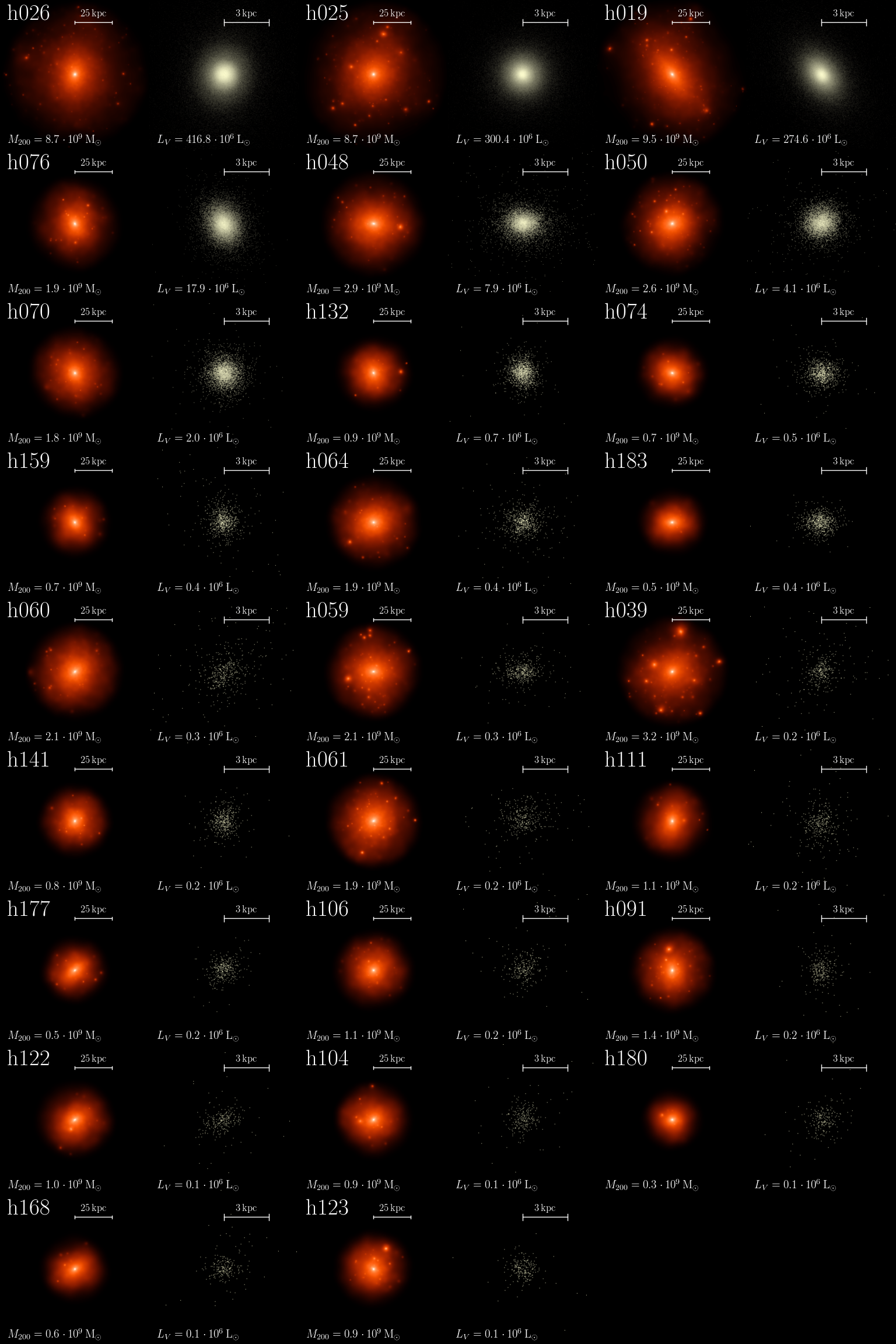
Figure 1: Catalogue of the 27 zoom-in haloes at $z=0$ with a final luminosity higher than $10^{5}\,\rm{L_{\odot}}$ corresponding to Local Group classical dwarfs. The dark halo surface density of each model truncated to its respective $R_{200}$ radius is shown with orangeish colours. The size of the box is $100\,\rm{kpc}$. A zoom on the corresponding stellar component, more precisely, the projection of the luminosity of each stellar particle is represented in yellowish colours. Here, the size of the box is $10\,\rm{kpc}$. The models are sorted from left to right and top to bottom according to their total luminosity.

Model ID	$L_{\rm{V}}$	$M_{\star}$	$M_{\rm{200}}$	$M_{\rm{gas}}$	$M_{\rm{cold\,gas}}^{r<r_{t},T<10^{4}\,\rm{K}}$	$M_{\rm{hot\,halo\,gas}}^{T\geq 10^{4}\,\rm{K}}$	$R_{\rm{200}}$	$r_{1/2}$	$\sigma_{\rm{LOS}}$	$\rm{[Fe/H]}$
	$[10^{6}\,\rm{L_{\odot}}]$	$[10^{6}\,\rm{M_{\odot}}]$	$[10^{9}\,\rm{M_{\odot}}]$	$[10^{6}\,\rm{M_{\odot}}]$	$[10^{6}\,\rm{M_{\odot}}]$	$[10^{6}\,\rm{M_{\odot}}]$	$[\rm{kpc}]$	$[\rm{pc}]$	$[\rm{km/s}]$	dex
h026	$451.12$	$537.84$	$8.71$	$460.04$	$195.37$	$262.64$	$49.2$	$1$	$32.3$	$-0.75$
h025	$309.37$	$520.16$	$8.67$	$246.10$	$83.15$	$162.50$	$49.1$	$1$	$30.6$	$-0.61$
h019	$291.39$	$433.92$	$9.53$	$280.17$	$99.06$	$180.72$	$50.7$	$0$	$30.5$	$-0.64$
h021	$233.79$	$334.81$	$6.83$	$183.01$	$142.43$	$235.68$	$45.4$	$1$	$28.1$	$-0.59$
h076	$18.56$	$38.33$	$1.88$	$22.96$	$14.09$	$8.70$	$29.5$	$0$	$13.3$	$-1.04$
h048	$8.02$	$13.71$	$2.92$	$26.53$	$9.70$	$16.75$	$34.2$	$0$	$11.2$	$-1.10$
h050	$4.16$	$9.56$	$2.62$	$15.11$	$3.48$	$11.62$	$33.0$	$0$	$10.4$	$-1.37$
h070	$2.02$	$5.83$	$1.83$	$0.01$	$0.00$	$0.01$	$29.2$	$0$	$10.8$	$-1.61$
h132	$0.75$	$2.10$	$0.90$	$0.52$	$0.00$	$0.52$	$23.1$	$0$	$9.3$	$-1.86$
h074	$0.50$	$1.35$	$0.69$	$0.39$	$0.00$	$0.39$	$21.2$	$0$	$9.1$	$-2.06$
h159	$0.42$	$1.07$	$0.67$	$0.01$	$0.00$	$0.01$	$21.0$	$0$	$8.9$	$-2.24$
h064	$0.41$	$1.07$	$1.88$	$5.16$	$0.00$	$4.92$	$29.5$	$0$	$9.7$	$-2.00$
h183	$0.37$	$1.00$	$0.54$	$0.02$	$0.00$	$0.02$	$19.5$	$0$	$8.6$	$-2.09$
h060	$0.27$	$0.69$	$2.06$	$3.70$	$0.00$	$3.69$	$30.4$	$0$	$10.4$	$-2.45$
h039	$0.27$	$0.64$	$3.24$	$17.18$	$0.00$	$17.18$	$35.4$	$1$	$11.7$	$-2.55$
h059	$0.26$	$0.67$	$2.07$	$4.25$	$0.00$	$4.24$	$30.5$	$0$	$9.3$	$-2.25$
h141	$0.22$	$0.58$	$0.76$	$0.47$	$0.00$	$0.47$	$21.8$	$0$	$8.3$	$-2.17$
h061	$0.22$	$0.53$	$1.93$	$3.45$	$0.00$	$3.44$	$29.8$	$0$	$9.1$	$-2.26$
h111	$0.20$	$0.49$	$1.09$	$0.11$	$0.00$	$0.07$	$24.6$	$0$	$10.4$	$-2.57$
h177	$0.19$	$0.49$	$0.54$	$0.01$	$0.00$	$0.01$	$19.4$	$0$	$7.7$	$-2.32$
h091	$0.17$	$0.40$	$1.36$	$0.84$	$0.00$	$0.83$	$26.5$	$0$	$10.1$	$-2.38$
h106	$0.15$	$0.37$	$1.09$	$0.08$	$0.00$	$0.08$	$24.6$	$0$	$9.9$	$-2.62$
h122	$0.14$	$0.36$	$0.97$	$0.01$	$0.00$	$0.01$	$23.7$	$0$	$9.1$	$-2.41$
h104	$0.14$	$0.34$	$0.92$	$0.28$	$0.00$	$0.27$	$23.3$	$0$	$9.0$	$-2.36$
h123	$0.13$	$0.34$	$0.91$	$0.05$	$0.00$	$0.05$	$23.2$	$0$	$7.6$	$-2.35$
h180	$0.12$	$0.30$	$0.29$	$0.01$	$0.00$	$0.01$	$15.9$	$0$	$6.9$	$-2.45$
h168	$0.12$	$0.29$	$0.56$	$0.02$	$0.00$	$0.02$	$19.7$	$0$	$8.3$	$-2.66$

Table 1: Properties of the 27 zoom-in dwarf galaxy models.

3.2 Generic evolution and properties of the multi-phase gas

To illustrate the formation and evolution of dwarf galaxies in our zoom-in simulations, Fig. 2 displays a few snapshots of the model h025 from $z=11$ down to $z=0$. The top panels show the evolution in the full cosmological box, with the refined regions identified by the gas distribution in blue. The bottom panels are magnifications of the dwarf itself.

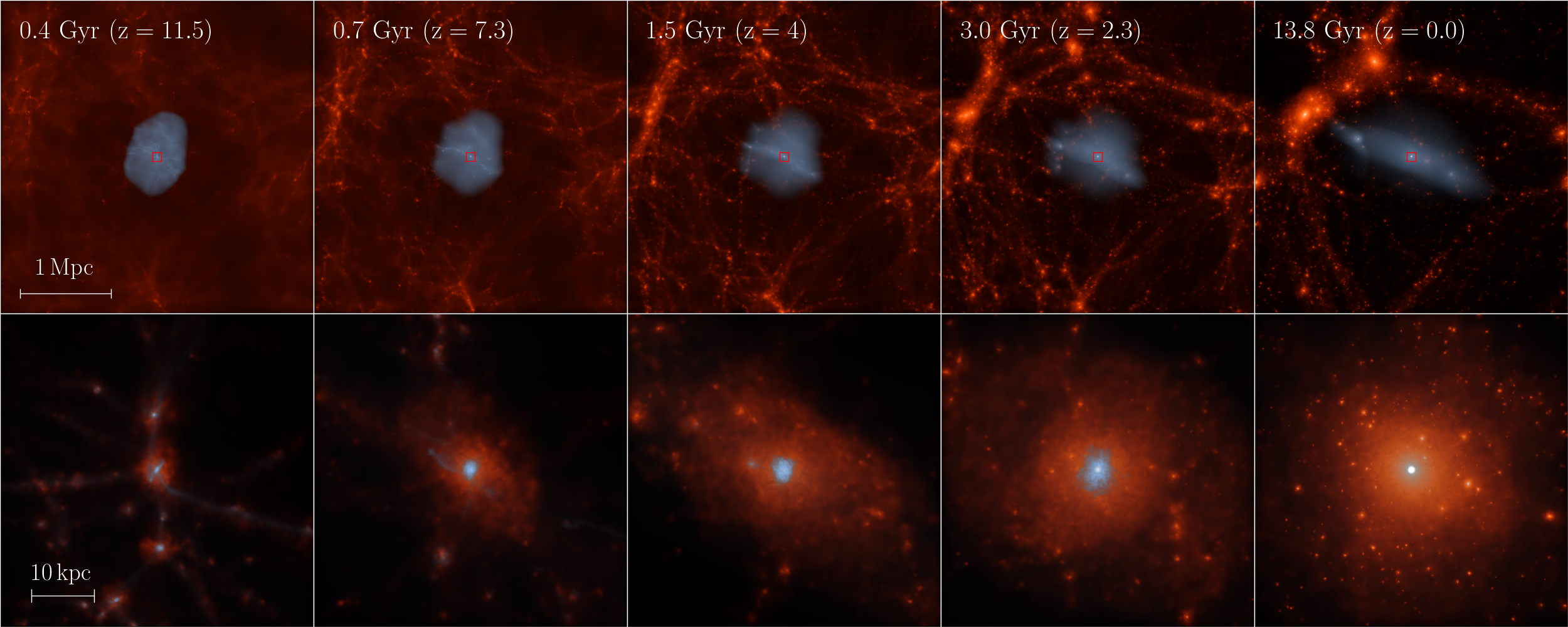
Figure 2: Evolution with time of the halo h025. The top panels display the evolution of the full $(3.4\,\rm{Mpc}/h)^{3}$ cosmological box. The red central squares identify the areas displayed in the bottom panels. In all quadrants, stars are shown in white, the gas is displayed in blue, and the dark matter in orange. The gas is only present in the regions which have been re-simulated at the highest resolution.

Figure 3 shows the distribution of the gas of model h025, in a $\log\rho$ vs $\log T$ diagram at a redshift of zero. Three gas phases are considered:

(i) the cold dense gas ($\rho\gtrsim 10^{-1}\,\rm{atom/cm^{3}}$, $T<1000\,\rm{K}$), (ii) the low density warm gas ($\rho\lesssim 10^{-3}\,\rm{atom/cm^{3}}$) forming a halo that can extend up to the virial radius of the dwarf, and (iii) the dense warm or hot gas ($\rho\gtrsim 10^{-1}\,\rm{atom/cm^{3}}$, $T>1000\,\rm{K}$). The cold phase of the gas arises from compression during the first collapse of the dark halo. Because of the hydrogen self-shielding, for density higher than $\sim 10^{-2}\,\rm{atom/cm^{3}}$, the cooling dominates and the gas temperature drops to $10\,\rm{K}$ which corresponds to the floor temperature adopted in the simulations. At this high density, the cold gas can form stars which in turn, via the feedback of the supernovae explosions, heats the gas up to $10^{5}-10^{6}\,\rm{K}$ forming the warm/hot phase. This over-pressurized gas expands and cools back adiabatically to very low temperature. A cycle between the cold and warm/hot phase is naturally maintained. For densities higher than about $10^{-1}\,\rm{atom/cm^{3}}$ the gas is then consequently multi-phase.

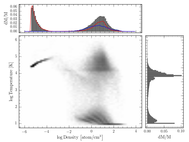
Figure 3: Distribution of the gas in $\log\rho$ versus $\log T$ for the model h025 at a redshift z=0. The intensity of the grey colour scales with the logarithmic of the 2-D mass-weighted histogram of the gas. The upper and right panels display the gas fraction as a function of its density and temperature, respectively. The red and the blue curves in the upper panel correspond to the warm/hot and cold gas distribution.

Figure 4 displays the surface density of the dense cold and dense warm/hot gas in a box of size of $1.5\,\rm{kpc}$. The cold gas appears very clumpy compared to the warm/hot one which is smoother. This underlines the fact that the gas is far from equilibrium as being continuously shaken by supernovae explosions that drives the formation of bubbles, inter-penetrating each-other. The gas distribution strongly homogeneous and stars are not restricted to form only in the inner few parsecs.

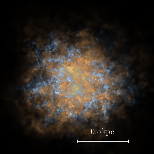
Figure 4: Surface density of the dense cold (in blue) and dense warm/hot (in orange) gas extracted from the model h025 at z=0.

A quick look a the line of sight of velocity dispersion of the gas show values of about $14\,\rm{km/s}$ for the cold phase, up to $17\,\rm{km/s}$ for the warm/hot phase. Less-massive systems display cold gas velocity dispersion lower than $10\,\rm{km/s}$.

3.3 Scaling relations

Our simulations are run in a cosmological context, however, they do not evolve under the influence of a massive host such as the Milky Way or Andromeda. Nevertheless, while the most detailed observational constraints can only be gathered in the Local Group, we see in the following that most of their observed features result from physical processes independently of any interaction with a central galaxy.

Our comparison sample is essentially based on the list of galaxies listed in the compilation of Local Group galaxies by McConnachie (2012). We restrict the sample to the satellites of the Milky Way and Andromeda galaxies brighter than $10^{5}\,\rm{L_{\odot}}$. We did not include the Sagittarius dSph as it is strongly stripped, making it difficult to get a census of its global properties.

3.3.1 Luminosity - velocity dispersion

Figure 5 displays the V-band luminosity of the simulated dwarf galaxies with respect to their line of sight stellar velocity dispersion, $\sigma_{\rm{LOS}}$, calculated as the velocity dispersion along a given line of sight of our stellar particles inside a $1\,\rm{kpc}$ cylindrical radius. For each galaxy, $\sigma$ is computed seven times, choosing different lines of sight. The quoted velocity dispersion is taken as the mean of the seven realizations and the error corresponds to their standard deviation. The predictions of our models are compared with a compilation of observations of both Milky Way and Andromeda galaxies as defined above.

Our model galaxies nicely reproduce the observed L_V-$\sigma$ relation over four order of magnitudes, from nearly $10^{9}\,\rm{L_{\odot}}$ down to $10^{5}\,\rm{L_{\odot}}$, corresponding to velocity dispersions of $35\,\rm{km/s}$ down to $7\,\rm{km/s}$. Thereby they provide insights on the origin of the diversity of formation histories, hence very different luminosities, of the systems with $\sigma_{\rm{LOS}}\lesssim 10\,\rm{km/s}$. Indeed, this results from the interplay between the build-up of the galaxy dark halo, the stellar feedback and the intensity of the UV-background heating during the re-ionization epoch. The primordial structures in the densest regions of the cosmic web merge on shorter timescales than those in more diffuse ones. Before the re-ionization epoch, the gas density of the former haloes is already high enough to be self-shielded against the coming UV-background. Moreover their potential well are deep enough to retain the fraction of gas which will be heated. These two factors prevent the star formation to be rapidly quenched (see Section 3.4) and the galaxies can reach luminosities up to $10^{7}\,\rm{L_{\odot}}$. In contrast, the formation timescale of galaxies in more diffuse regions is longer. As a consequence, the final halo is not yet assembled at the onset of the re-ionization epoch. It leaves the constitutive sub-haloes with shallow potential well. The gas is not self-shielded anymore and can evaporate, hence the star formation quickly stops, building very low luminosity systems down to $10^{5}\,\rm{L_{\odot}}$ or even lower in the regime of UFDs. In the most extreme cases, the stellar feedback by itself is sufficient to considerably reduce the star formation rate even before the re-ionization epoch.

These mechanisms lead to a non-monotonic relation between dark mater haloes and their stellar content. Consequently, the assumption of abundance matching between dark halo and stellar masses (Moster et al., 2010; Guo et al., 2010; Sawala et al., 2011; Behroozi et al., 2013; Moster et al., 2013) breaks down below $\sim 10\,\rm{km/s}$. In the simulations of Sawala et al. (2015) the dispersion in luminosity at given halo mass originated from the interaction between the the Milky Way and its satellites. Here, we show that the assembly of the dwarf systems itself is sufficient to generate this scatter.

While we do not produce systems with velocity dispersions below $5\,\rm{km/s}$ such as the six Andromeda satellites, we note the large uncertainties on their velocity measurement and the absence of similar systems around the Milky Way. It is worth noting that there is a dearth of models in the luminosity range $2\times 10^{7}$ to $2\times 10^{8}\,\rm{L_{\odot}}$. We can only attribute this dearth to a lack of statistics.

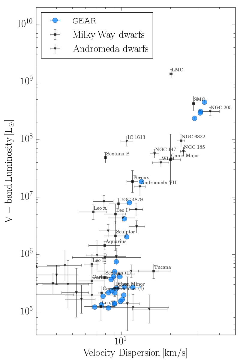
Figure 5: Galaxy V-band luminosity versus its stellar line-of-sight velocity dispersion. The blue circles correspond to the predictions of the simulations, while the back squares and triangles stand for the Milky Way’s and M31 satellites respectively (see Section 3.3 for the references). For clarity, we only label the M31 satellites brighter than $10^{7}\,\rm{L_{\odot}}$.

3.3.2 Metallicity - luminosity

Figure 6 displays the median of the stellar metallicity distribution ($\rm{[Fe/H]}$) of each dwarf model galaxy, as a function of its V-band luminosity ($L_{\rm{V}}$). The error bars correspond to the difference between the mode and the median of the $\rm{[Fe/H]}$ distribution. Our models are compared with our Local Group sample of galaxies, restricting to galaxies that benefit from medium resolution spectroscopy with metallicity derived either from spectral synthesis or Calcium triplet (CaT) calibration.

Our models again match the observations over four dex in luminosities. Though, below $10^{6}\,\rm{L_{\odot}}$ there is a tail of faint dwarfs which have a median metallicity below the observed range. Given the fact that those systems have correct luminosities and velocity dispersions, this discrepancy most likely arises from the fact that our IMF and yields are kept constant all along the simulations. A more detailed model should consider POP III stars with a different IMF (Bromm, 2013) and yields (Iwamoto et al., 2005; Heger & Woosley, 2010), as assumed in some other studies (Verbeke et al., 2015; Salvadori et al., 2015; Jeon et al., 2017). This could play a role, in particular, for the very first generation of stars and more strongly impact the smallest systems. Another point is that we have here some of the lightest haloes which could well be disrupted by the proximity of a massive galaxy through tidal stripping. A similar trend has been found in Oñorbe et al. (2015); Wetzel et al. (2016) and Macciò et al. (2017) at even higher luminosities.

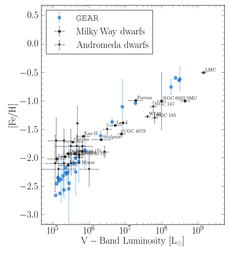
Figure 6: Galaxy mean metallicity ($\rm{[Fe/H]}$) as a function of its final V-band luminosity ($L_{\rm{V}}$). The blue circles corresponds to the model predictions, for which $\rm{[Fe/H]}$ is computed as the median of the galaxy stellar metallicity distribution function. The error bars correspond to the difference between the mode and the median values of this distribution. The Milky Way and M31 satellites, with reliable $\rm{[Fe/H]}$ determination (see text for details), are identified with black squares and triangles, respectively. For clarity, we only label the M31 satellites brighter than $10^{7}\,\rm{L_{\odot}}$.

3.3.3 Size - luminosity

Figure 7 presents the relation between the half light radius ($r_{1/2}$) and the V-band luminosity for our model galaxies. For each of our dwarf, we first removed any contamination from sub-haloes containing stars, falling within its $r_{200}$. This was performed with a halo finder following the SUBFIND algorithm (Springel et al., 2001). Then, we fitted a modified King model to the projected radial stellar profile:

$$I(R)=\frac{I_{0}}{\left(1+(R/R_{c})^{2}\right)^{a}}+b,$$ (4)

where $I_{0}$ is the central surface brightness of the standard King model, $R_{c}$ is the core radius, $a$ sets the outer slope, and $b$ represents some background noise. We measured the total luminosity within a radius which is defined as the one at which the background noise dominates. Concretely, this is set when the fitted profile deviates from more than $0.5\%$, in logarithmic scale, from the profile without noise ($b=0$). The half light radius is then the projected radius containing half the total luminosity.

The upper panel of Fig. 7 shows the result of this calculation at $z=0$. Above $10^{6}\,\rm{L_{\odot}}$, our models fall within the range of the observed values. Moving below $10^{6}\,\rm{L_{\odot}}$, the mean $r_{1/2}$ of the models is kept nearly constant, thereby staying at the level of the upper envelope of the galaxy observed sizes. The lower panel of Fig. 7 shows the same $r_{1/2}$ - luminosity relation when the size of the galaxies are calculated soon after the quenching of their star formation when this happens, that is essentially for the faintest systems.

The agreement between the models and the observations is clearly improved, for the following reason: both dark matter and stellar components are sampled with live particles in the simulations. These particles interact and exchange linear and angular momentum. As stars originates from the gas, they inherit their velocity dispersion, which is slightly smaller than that of the dark halo. The energy exchange between the dark matter and the stars is subsequently possible leading to dynamical heating of the stars. This results in the secular flattening of the central stellar component and therefore increases $r_{1/2}$. This effect is a direct consequence of the resolution of our simulations and more generally of any similar modelling. Would the dark matter be simulated as a perfectly smooth component, either as a fixed potential or with an extremely high resolution, this heating would disappear. We could also have set the gravitational smoothing length to very large values, however this would have affected all the dynamics of the systems. It is worth noting that such heating mechanism is akin to the one described by Jin et al. (2005), where a dark halo is composed of massive black holes. We stress that we have discarded all other possible source of heating, either spurious numerical ones, namely (i) dynamical heating due to too small a gravitational softening length, (ii) inaccuracy of the gravity force in the treecode, (iii) non-conservation of momentum at the time of the supernova feedback, as well as physical ones such as (i) a continuous accretion of small dark haloes, (ii) an adiabatic expansion due to the quick gas removal resulting from the UV-heating, (iii) a continuous mass loss of the stellar population.

It is still true that our models do not reach the same compactness as some of the observed dwarfs, such as Leo T or Andromeda XVI with a half light radius as small as $100\,\rm{pc}$. This discrepancy is also faced by other groups as for example Fitts et al. (2017), Macciò et al. (2017), or Jeon et al. (2017) who explore the domain of ultra-faint dwarf galaxies. Hence, it seems that this is a genuine problem of $\Lambda$CDM simulations which deserves further investigation.

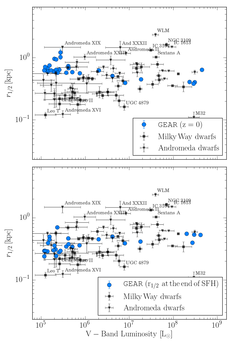
Figure 7: Galaxy half-light radius as a function of its final V-band luminosity ($L_{\rm{V}}$). The blue hexagons show the model predictions at z=0 (top panel) or soon after the end of the star formation activity (bottom panel). The Milky Way and M31 satellites are identified with black squares and triangles, respectively. For clarity, we only label galaxies with extreme half light radius, larger than $1\,\rm{kpc}$ or smaller than $200\,\rm{pc}$.

3.3.4 Gas mass - luminosity

Figure 8 displays the relation between the mass of the different gas phases and the final V-band luminosity of the model galaxies. The models are compared to the HI gas masses of the Local Group galaxies provided by McConnachie (2012). Although denser and colder components can be present, HI remains the dominant gas component, by a factor of approximately five, of the dwarf systems (Cormier et al., 2014).

Extracting the different gas phases, H2, HI, and HII, requires targeted procedures, which are not yet implemented in GEAR (see for example De Rijcke et al., 2013; Crain et al., 2017). For the sake of our present purpose, we extracted for each model galaxy cold and hot halo gas component. The cold gas component ($T<10^{\prime}000\,\rm{K}$) is define here as the neutral gas component and shares the same extension as the stars. The hot halo gas ($T\geq 10^{\prime}000\,\rm{K}$) extends much further and we have derived its mass up to the virial radius, as reported in Table 1. While all models show the presence of hot gas, we stress that this gas will be easily removed by ram pressure stripping while dwarfs orbit around their host galaxy.

Model galaxies above $L_{\rm{V}}>10^{7}\,\rm{L_{\odot}}$ are able to keep their cold gas and can still form stars up to z=0 (see Section 3.4). We only have three models in the luminosity range $L_{\rm{V}}=10^{6}$ to $L_{\rm{V}}>10^{7}\,\rm{L_{\odot}}$ (h048,h050,h070) and two of them still have cold gas in agreement with the observations. Between $L_{\rm{V}}=10^{5}$ and $L_{\rm{V}}>10^{6}\,\rm{L_{\odot}}$ our models are lacking the gas which is expected from the observations. Larger dark matter haloes would have deeper potential wells and would therefore retain their gas more easily. However, correct modelling of the luminosities and metallicities of these galaxies would then require the use of a stronger supernovae feedback. This would result in velocity dispersions too high to be compatible with the observations. Given the fact that our feedback is already low, the most likely source of this dearth of cold gas is the intensity of the UV-background at the origin of the gas heating.

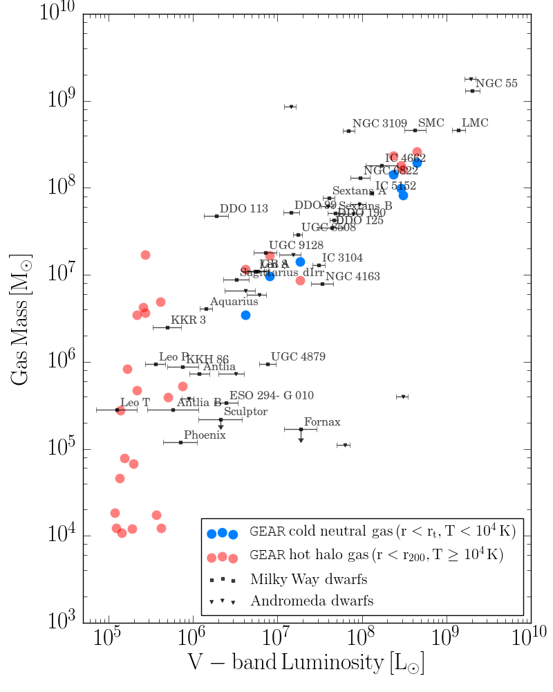
Figure 8: Galaxy gas mass content versus its V-band luminosity at z=0. For all galaxies, if present, the cold neutral gas phase ($T<10^{\prime}000\,\rm{K}$) found inside the tidal radius $r_{\rm{t}}$ is shown with blue circles. The red circles corresponds to the hot halo gas ($T>10^{\prime}000\,\rm{K}$) which extend up to the virial radius $r_{200}$. For comparison, the mass of neutral hydrogen (HI) observed in some of the Milky Way and M31 satellites is shown in black. For Sculptor and Sextans we used the upper limits detection values as given by McConnachie (2012).

3.4 Star formation histories

The galaxy star formation rates have a $\sim 100\,\rm{Myr}$ periodicity which results from the global pulsation of the systems as a direct consequence of the supernovae feedback. All galaxies display an additional short timescale variation. For the faintest systems, the periods of star formation interruption occur over a timescale of about $10\,\rm{Myr}$. This timescale is reduced to $0.5\,\rm{Myr}$ for the most luminous systems, as a consequence of the strong inhomogeneity of the ISM (see Section 3.2). Indeed, despite a strong supernova feedback boosted by an adiabatic phase (Stinson et al., 2006), some regions of the dwarfs include dense and cold clumps of gas that can turn into stars at nearly all times.

As expected, the final luminosity ($L_{\rm{V}}$) of our model dwarfs strongly correlates with the shape of their formation histories. We divide our models into three categories dependent on their $L_{\rm{V}}$ range. In the following we will refer to them as sustained, extended and quenched. A few representative cases of each of these three categories are shown in Fig. 9. The strength of the UV-background heating is indicated by the dotted black curve. It represents the hydrogen photo-heating rate due to the UV-background photons following the model of Haardt & Madau (2012).

• (a) $L_{\rm{V}}>10^{8}\,\rm{L_{\odot}}$, sustained: The star formation rate of those massive and luminous dwarfs increases over $1$ to $2\,\rm{Gyrs}$. This period is followed by a rather constant SFR plateau. These systems are massive enough to resist the UV-background heating and, once formed, to form stars continuously . This sustained star formation activity that lasts up to $z=0$ results from the self-regulation between stellar feedback and gas cooling (Revaz et al., 2009; Revaz & Jablonka, 2012).

• (b) $10^{6}\,\rm{L_{\odot}}<L_{\rm{V}}<10^{8}\,\rm{L_{\odot}}$, extended: In this luminosity range, the star formation is clearly affected by the UV-background. After a rapid increase, the star formation activity is damped owing to the increase of the strength of the UV-heating. However, at the exception of the h070 halo which is definitively quenched after $6.5\,\rm{Gyr}$, the potential well of those dwarfs is sufficiently deep to avoid a complete quenching. The star formation activity extends to $z=0$, however, at a much lower rate than the original one.

• (c) $L_{\rm{V}}<10^{6}\,\rm{L_{\odot}}$, quenched: The potential well of those galaxies is so shallow that the gas heated by the UV photons escape the systems. Star formation is generally rapidly quenched after $2$ or $3\,\rm{Gyr}$. Only halo h064 shows signs of activity up to $4\,\rm{Gyr}$. Those galaxies may be considered as true fossils of the re-ionization in the nomenclature of Ricotti & Gnedin (2005). They are all faint objects with only old stellar populations.

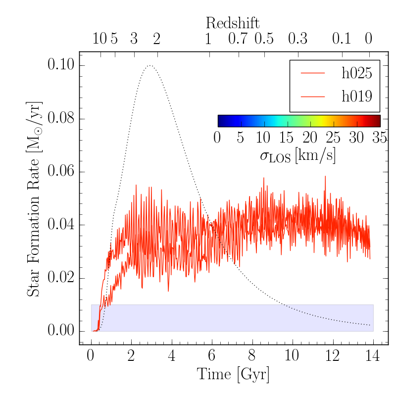
(a) $L_{\rm{V}}>10^{8}\,\rm{L_{\odot}}$ : sustained

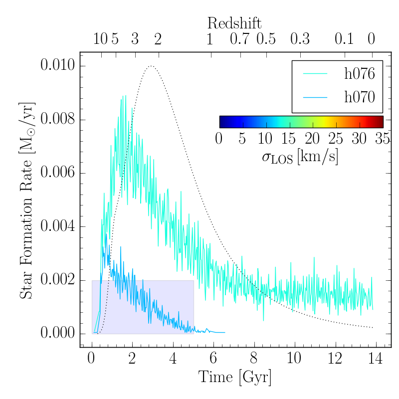
(b) $10^{6}\,\rm{L_{\odot}}<L_{\rm{V}}<10^{8}\,\rm{L_{\odot}}$ : extended

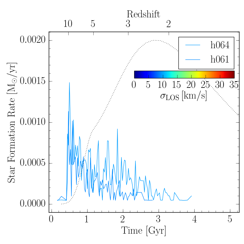
(c) $L_{\rm{V}}<10^{6}\,\rm{L_{\odot}}$ : quenched

Figure 9: The three categories of star formation histories observed: sustained, extended and quenched. The colours code the model galaxy velocity dispersion. The dotted black curves show the redshift dependent hydrogen photo-heating rate due to the UV-background photons. The curves are normalized so that the peak of the photo-heating rate coincides with the top of the y-axis. To illustrate the change in intensity and length of the star formation histories between the three categories, the shaded rectangles in panel (a) and (b) have dimensions corresponding to the maximal x and y-axis extensions of the panels (b) and (c), respectively.

3.5 Detailed stellar properties of local group dSphs

In this section, we go one step further by investigating whether the models emerging from our zoom-in $\Lambda$CDM simulations not only reproduce the galaxy integrated properties over several dex in luminosities, but also match their detailed stellar properties, such as velocity dispersion profiles, stellar metallicity distribution, and abundance ratios.

For each class of model star formation history (sustained, extended, quenched), we have looked for well documented Local Group dwarf galaxies. One of our stringent criterion was the availability of a significant number of stars observed at high resolution ($R>15^{\prime}000$). This is indeed essential to derive accurate chemical abundances. In the following, we will particularly focus on magnesium and iron.

For the quenched galaxies, we have selected Sextans, Ursa Minor and Draco. Andromeda II and Sculptor, for which a $6$ to $8\,\rm{Gyr}$-long star formation history has been derived (Weisz et al., 2014a; Skillman et al., 2017; de Boer et al., 2012a) are our comparison galaxies for the extended star formation cases. Only few observed systems fall in the range of luminosity and metallicity of the sustained class of our models. NGC 6822 seems to be the best match in the global relation diagrams. Unfortunately these massive systems are also more distant and do not possess high resolution spectroscopic follow-up. We have not considered the LMC and SMC because of their mutual interaction which evidently affected their evolution.

Failures can be as informative as successes. In this regard, we point out that two well documented galaxies do not match any of our model star formation histories, the Carina and Fornax dSphs. Carina is known for its distinct episodes of star formation with the majority of its stellar mass formed at intermediate ages (Hurley-Keller et al., 1998; Weisz et al., 2014a; de Boer et al., 2014; Kordopatis et al., 2016; Santana et al., 2016). Moreover, The Carina Project has recently demonstrated the complex structure of its velocity dispersion, potentially arising from strong gravitational disturbances (Fabrizio et al., 2011, 2016). The population of Fornax is dominated by intermediate age stars and stars as young as $200\,\rm{Myr}$ are also present (Coleman & de Jong, 2008; Saviane et al., 2000; de Boer et al., 2012b). The very peculiar star formation histories of these Carina and Fornax could be the consequence of a strong interaction with a massive host galaxy as proposed by Pasetto et al. (2011) for Carina, and indeed we have none in our cosmological volume. The comparison between the six selected dSphs and the models matching the galaxy total V-band luminosity, stellar line of sight velocity dispersion, stellar metallicity distribution, and when available, their [Mg/Fe] ratio (where Mg is used as a proxy for $\alpha$-elements), is provided in Fig. 10.

For each dSph, the lower left panel compares the line of sight velocity dispersion profile of the model (blue curve) with the observations in red. In addition, we display in black the model total circular velocity. For NGC 6822 the line of sight velocity dispersion have been determined by Tolstoy et al. (2001), Kirby et al. (2013) and Swan et al. (2016) with values ranging between $23.2\,\rm{km/s}$ and $24.5\,\rm{km/s}$. We adopted a value of $24\,\rm{km/s}$ with a reasonable error bar of $\pm 2\,\rm{km/s}$. For Andromeda II, we took the x-axis velocity dispersion profile of Ho et al. (2012). For Sculptor and Sextans, we used the publicly available radial velocity measurement of Walker et al. (2009a) and only kept stars with a membership probability larger than $90\%$. For those two galaxies, we could, just as for the models, directly derive the luminosity weighted line of sight velocity dispersion in circular logarithmic radial bins. Because the size of the bins increases with galacto-centric distances, the noise is reduced at larger radii. For Draco and Ursa Minor, the profile is obtained by by-eye fitting the plots of Walker et al. (2009b) assuming a constant error of $2\,\rm{km/s}$.

The upper right panel of Fig. 10 provides the comparison between the model and the observed stellar metallicity distribution functions. For NGC 6822, the metallicity distribution comes from Swan et al. (2016). For Andromeda II we inferred it ourselves from the sample of Vargas et al. (2014). Finally, for Sextans, Sculptor, Ursa Minor and Draco, we retrieved the $\rm{[Fe/H]}$ values from the SAGA database (Suda et al., 2008), thanks to a series of original works on Ursa Minor (Shetrone et al., 2001; Sadakane et al., 2004; Cohen & Huang, 2010; Kirby et al., 2010), Draco (Shetrone et al., 2001; Cohen & Huang, 2009; Kirby et al., 2010; Tsujimoto et al., 2015), Sculptor (Battaglia et al., 2008; Kirby et al., 2010; Lardo et al., 2016), Sextans (Kirby et al., 2009, 2010; Battaglia et al., 2011).

The lower right panel compares the model and observed [Mg/Fe] vs $\rm{[Fe/H]}$ trends. The abundance of magnesium and iron have been retrieved from the works quoted above for Ursa Minor and Draco. For Sculptor we compiled the works from Shetrone et al. (2003); Tafelmeyer et al. (2010); Tolstoy et al. (2009); Jablonka et al. (2015). For Sextans, we benefited from Shetrone et al. (2001); Aoki et al. (2009); Tafelmeyer et al. (2010); Theler (2018).

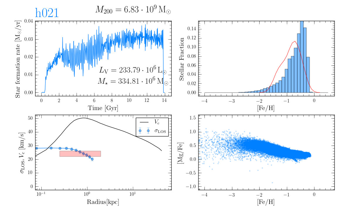
(a) NGC 6822

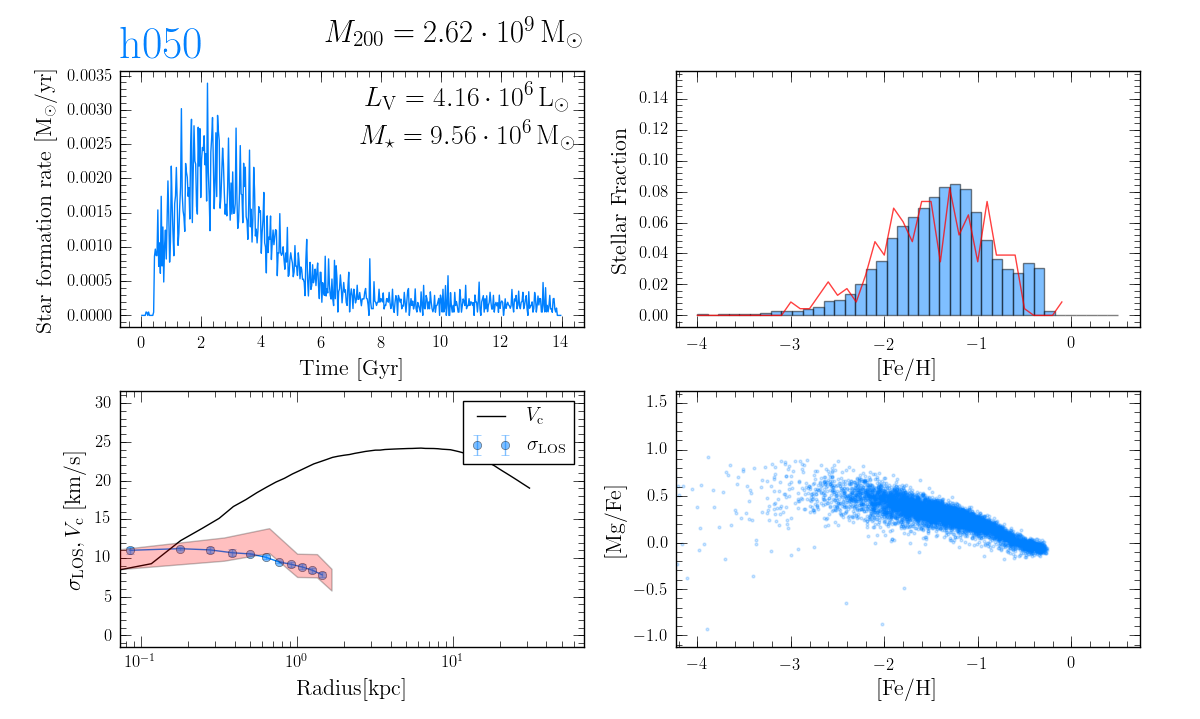
(b) Andromeda II

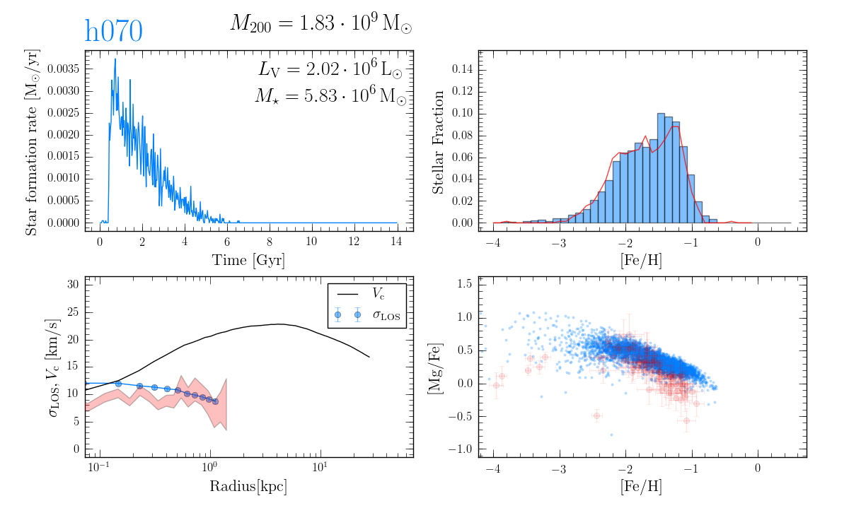
(c) Sculptor

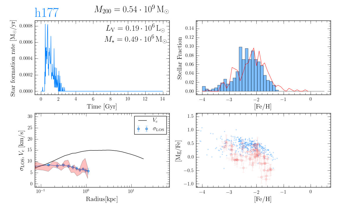
(d) Sextans

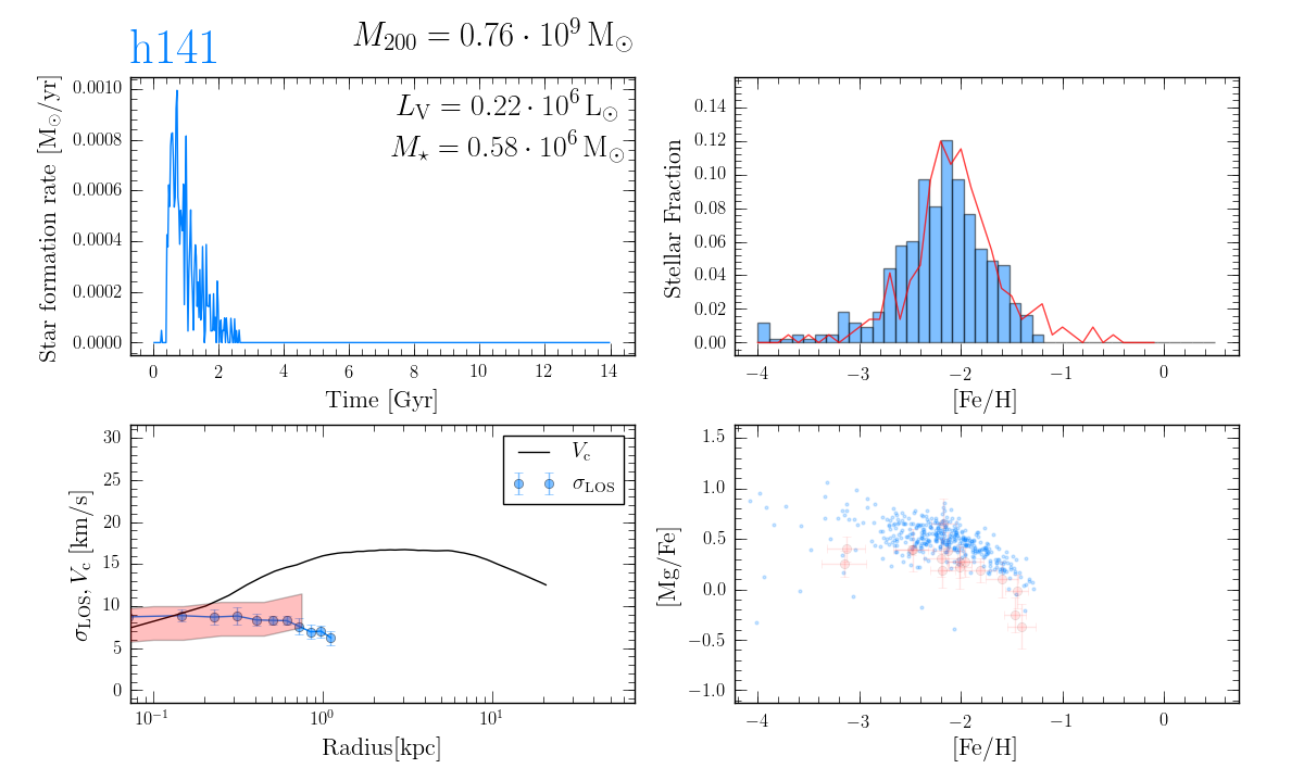
(e) Ursa Minor

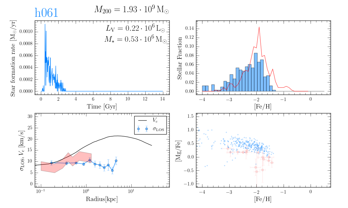
(f) Draco

Figure 10: Comparison of the stellar properties of the six Local Group dwarf galaxies: NGC 6822, Andromeda II, Sculptor, Sextans, Ursa Minor and Draco. The model id, the model galaxy total mass ($M_{200}$), total luminosity ($L_{\rm{V}}$), and total stellar mass ($M_{\star}$), which are calculated inside the virial radius $R_{200}$ are indicated on the upper left hand side of each series of four panels. For each galaxy, the upper left panel displays the model star formation history. The lower left panel shows the line of sight velocity dispersion of the model galaxy in blue, as compared to the observations (red shaded area). The black line corresponds to the total circular velocity. The upper right panel displays the model galaxy stellar metallicity distribution. The lower right panel gives the galaxy [Mg/Fe] vs [Fe/H] distribution. In both quadrants, the model is seen in blue and the observations in red.

Admittedly, this is the first time that models arising from a $\Lambda$CDM cosmological framework and their physical ingredients are checked in such a detail and they do indeed match the observations well. The six observed dwarfs, chosen as test-beds, which sample a large variety of star formation and merger histories, chemical evolutions, and velocity dispersions, are remarkably well reproduced. Some matches could have most likely been slightly improved had we benefited from a larger sample of simulated galaxies, in other words, a larger cosmological volume. An obvious example is provided by NGC 6822 for which the model luminosity and peak of the stellar metallicity distribution are both slightly too high. As we mentioned earlier we faced a lack of models in this luminosity and metallicity range. It is worth mentioning that our Sculptor model predicts a maximal velocity of about $23\,\rm{km/s}$ in perfect agreement with the recent predictions of Strigari et al. (2017).

Figure 10 also points out how challenging it is to observationally derive reliable total halo masses for dwarf galaxies. Indeed, while model h141 and h061 share similar luminosities, star formation histories, mean metallicities and velocity dispersions, their virial halo masses differ by more than a factor of 2.5. Likewise, the models h061 and h070 have similar virial masses, however very different stellar properties. To shed light on these diverging properties, we computed the time evolution of the virial and stellar mass of those three models.

During the first Gyr, h141 has a slightly higher virial mass allowing to form about twice as much stars as h061. However later on, h061 experiences two important accretion events. The first event double the dwarf dark mass, without gaining neither gas nor stars, as only small dark haloes devoted of baryons are swallowed. Later on, the dwarf double its mass once more by merging with a smaller dwarf which also adds stars and gas. Those two events occurs after the decrease of the star formation due to UV-background heating. Hence, despite a different assembly history, the star formation history of models h061 and h141 are similar. Compared to model h061, model h070 is assembled much quicker which helps it to resist the UV-background heating and extend its star formation history . This different assembly histories echoes the large scatter of the luminosity - velocity dispersion relation found in Section 3.3.1.

3.6 Metallicity and age gradients

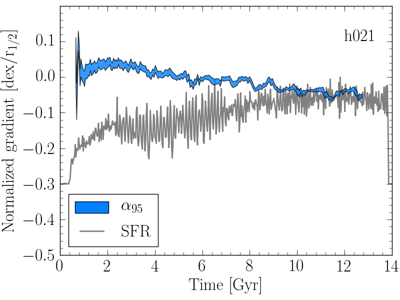
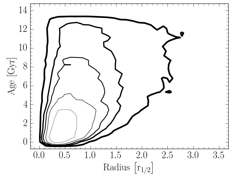
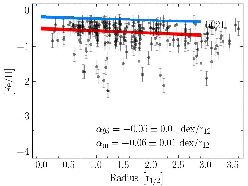
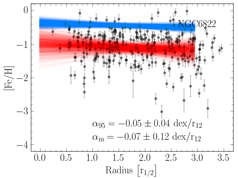
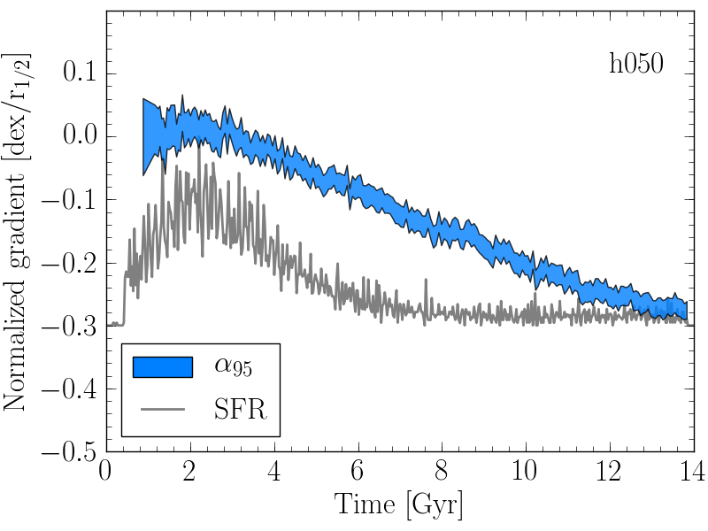
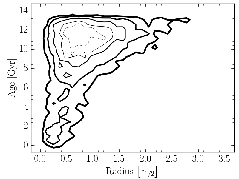
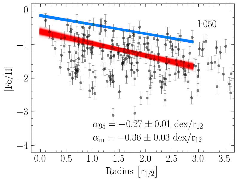
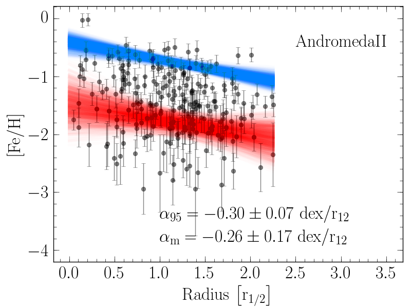
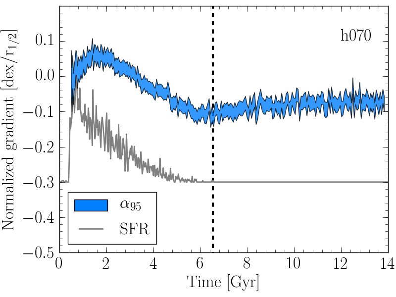
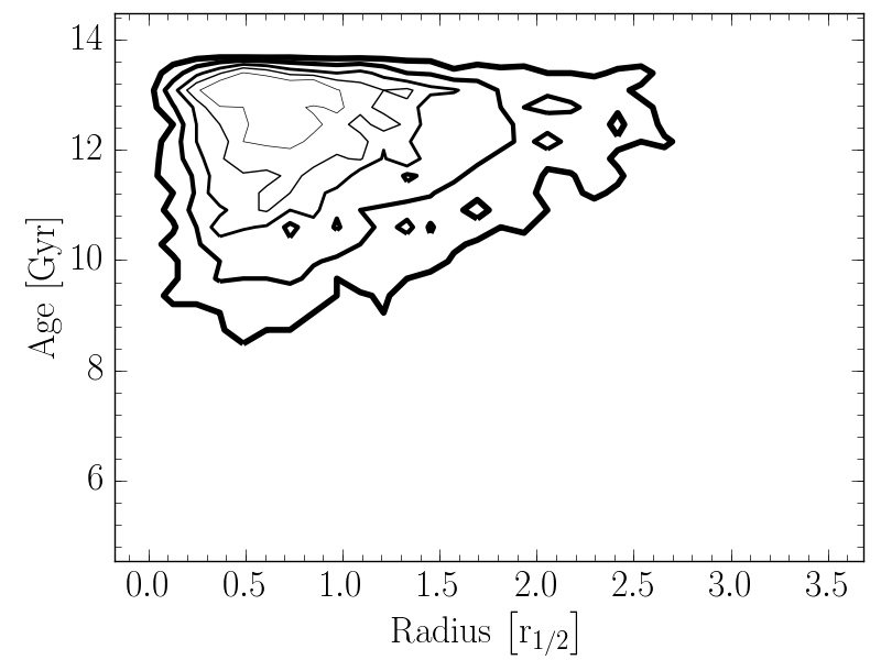
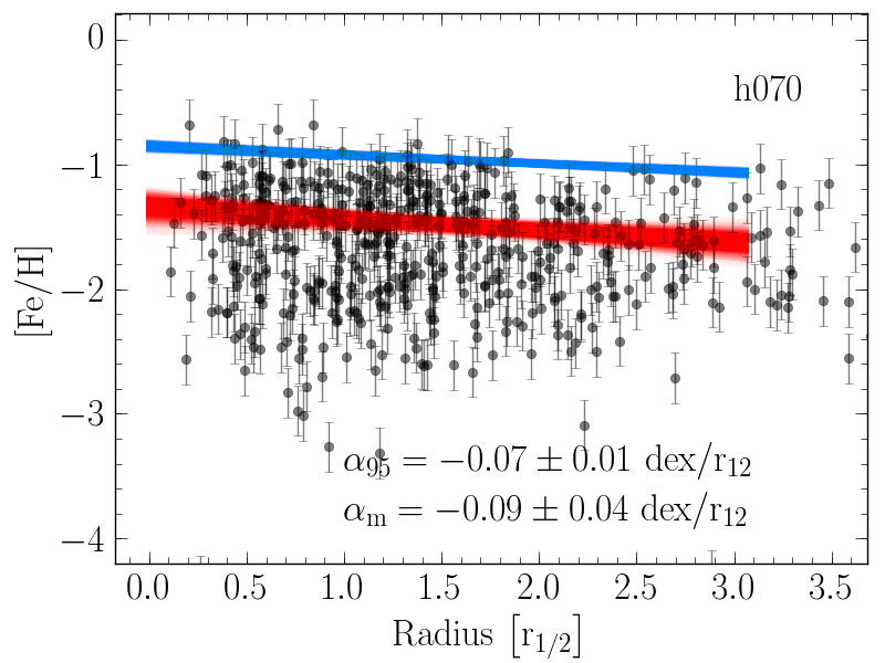
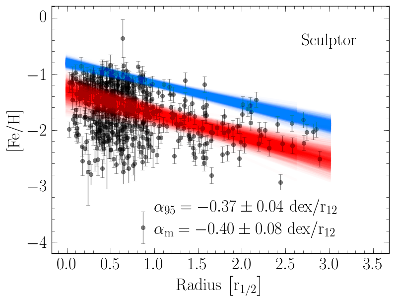
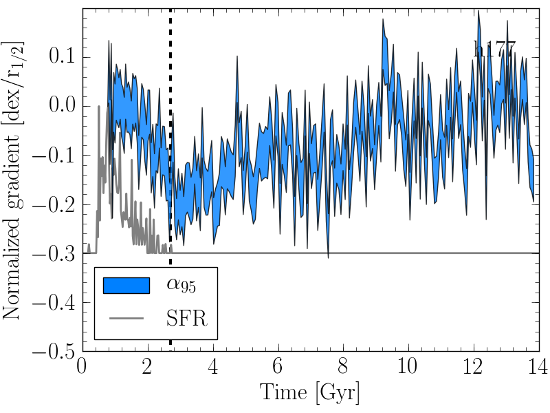
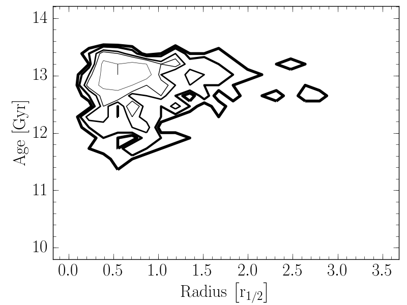
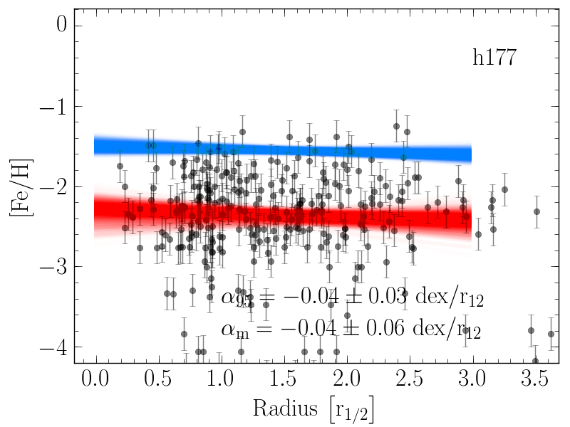
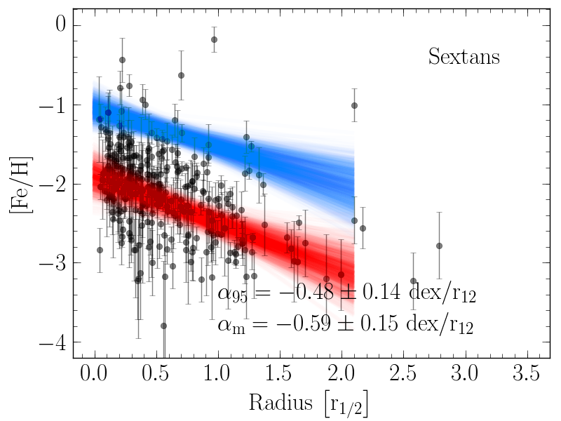
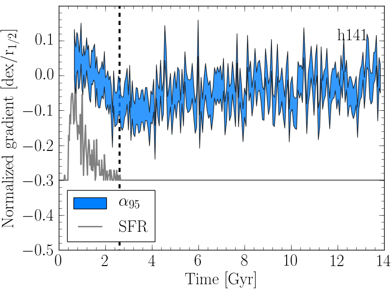
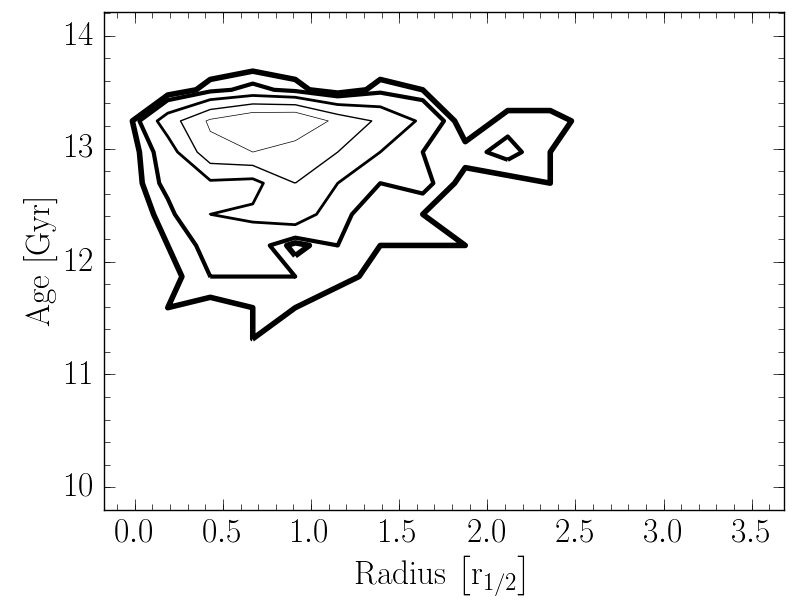
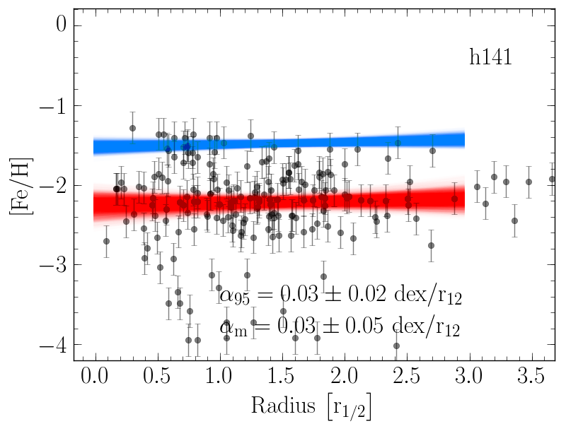
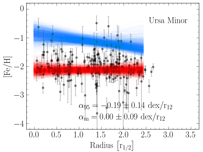
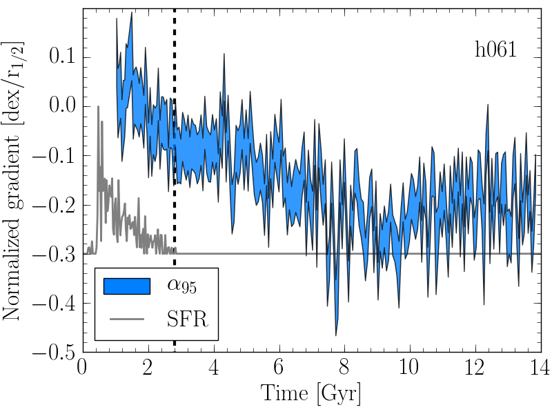
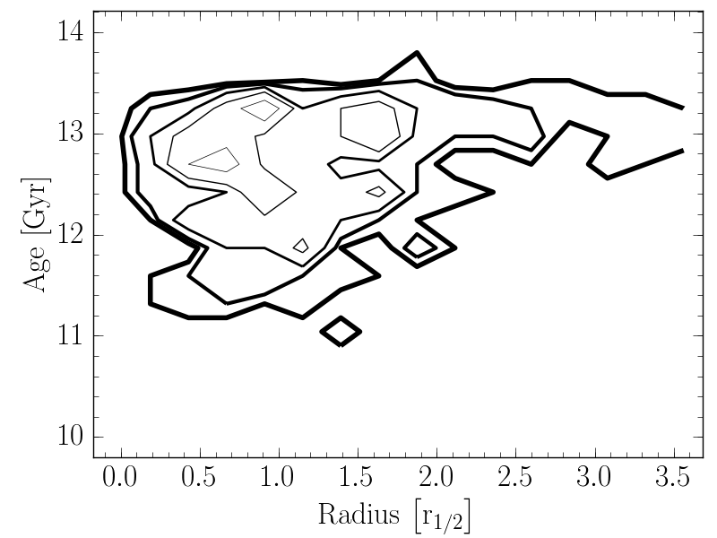
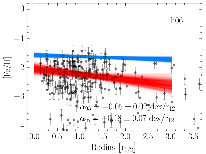
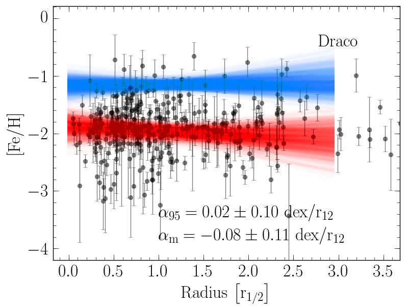
Figure 11: Metallicity and age gradients of the simulated dwarf galaxies as compared to the observations. The first column shows the time evolution of the normalized $\rm{[Fe/H]}$ gradients determined by the 95th percentile ($\alpha_{95}$, in blue) of the model galaxy stellar metallicity distribution. The width of the curve traces the error on the slopes (see text for details). The grey curve corresponds to the normalized star formation rate and, when displayed, the vertical dashed line indicates the end of the star formation period. The second column shows the age distribution of the stars in as function of the galaxy projected radius. The third and fourth columns compare the metallicity gradients of each model at z=0 , to a corresponding observed galaxy. The red and blue lines correspond to the fit of the mode (red) and 95th percentile (blue) of the observed and model stellar metallicity distributions. Their width reflect the uncertainty on the slope. The values of $\alpha_{\rm{m}}$ and $\alpha_{95}$ together with their error bars are provided. For a fair comparison, the number of stars in the model and in the observed are equal.

Stellar metallicity and gradients are quite common in the Local Group dSphs. For example they have been reported in Sculptor, Fornax, Sextans, Carina, Leo I, Leo II, NGC 185, and Andromeda I-VI (Harbeck et al., 2001; Tolstoy et al., 2004; Battaglia et al., 2006, 2011; Kirby et al., 2011; de Boer et al., 2012a, b; Vargas et al., 2014; Ho et al., 2015; Lardo et al., 2016; Okamoto et al., 2017; Spencer et al., 2017)

However, only a few physical interpretations have been put forward to explain these structured age and metallicity radial changes. Suggestions have been made that they could form either secularly, from the centrally concentrated star formation (Schroyen et al., 2013) or more recently by a late gas accretion which could reignite star formation in the galaxy central regions (Benítez-Llambay et al., 2016). The metal-poor stars could have been scattered over large galacto-centric distances either by successive merger events at high redshift (Benítez-Llambay et al., 2016) or by recurrent strong stellar feedback, pushing away the dark matter and driving stars on less bound orbits (Pontzen & Governato, 2014).

Figure 11 illustrates the formation of these gradients in our models in comparison with the observations. We first describe the procedure we applied to both observed and model galaxies. Stars or stellar particles were first considered in a $\rm{[Fe/H]}$ vs projected and normalized galacto-centric radius space. The normalization was done to the half-light radius of the model dwarf, as often the case for the observations. As to our simulations, this also avoids to introduce a bias owing to the dynamical heating described in Section 3.3.3.

While we use the terminology gradient, a more accurate description should probably be that the metal-poor stars are evenly distributed from the central galaxy regions to the outer ones, while the most metal-rich populations are more spatially concentrated (see also Battaglia et al., 2011). Therefore characterizing the radial variation of the upper envelope of the stellar metallicity distribution is often more appropriate than a classical radial linear fit. Consequently, we computed the metallicity distribution function in 20 radial bins and, for each of them, determined both their mode and 95th percentiles. We further performed a linear fit of those values versus the projected radii. The slopes of these fits are $\alpha_{\rm{m}}$ and $\alpha_{95}$, respectively. They are taken as a proxy for the normalized metallicity gradients. We used a Monte Carlo approach to estimate the errors on the slopes. For each star or stellar particle, we varied their metallicity a thousand times following a Gaussian distribution centred on their mode metallicity or percentile with a dispersion corresponding to their uncertainties. For the observed galaxies, $\rm{[Fe/H]}$ and their corresponding errors were taken from the SAGA database (Suda et al., 2008). For the models we adopted a fiducial error of $\rm{[Fe/H]}$ of $0.2\,\rm{dex}$ which corresponds to a typical observational uncertainty. The final slopes $\alpha_{\rm{m}}$ and $\alpha_{95}$ are the mean and their error bar the standard deviation of the thousand fits. We note that $\alpha_{95}$ leads to less noisy behaviour compared to $\alpha_{\rm{m}}$.

For each of the galaxies presented in Fig. 10, Fig. 11 provides the time evolution of $\alpha_{\rm{m}}$ and $\alpha_{95}$, as well as the spatial distribution of the stellar ages and metallicities of the models. The latter is compared to the observations. For non-rotating objects, the strength of the gradients is primarily linked to the length of the star formation history. Systems with an extended star formation history exhibit stronger gradients than those which have been early quenched. Nevertheless, in case of fusions, the quenched systems can still exhibit relatively strong gradients, as we will describe further below. Luminous systems that formed through sustained star formation do rotate, and exhibit only very weak gradients.

The first column of Fig. 11 shows that the radial distribution of metals traced by $\alpha_{95}$ varies with time, in relation with the galaxy star formation history. They stay generally nearly constant once star formation has ceased. In some cases, however, and for isolated galaxies, one sees a slight decrease of these gradients as the consequence of the mixing of the different stellar populations induced by their velocity dispersion. In the case of a merger event, again once star formation has stopped, the situation is different. For example, model h061 merges at about $6\,\rm{Gyr}$ with a lower mass and lower metallicity system. The metal-poor stars of this small impacting body is dispersed in the outer regions of h061. This increases the global metallicity gradient for a couple of Gyrs, after which it decreases again due to the stellar mixing.

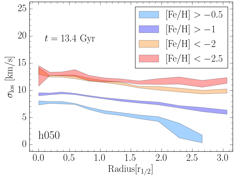
(a) h050 (Andromeda II)

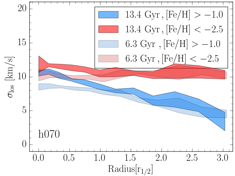
(b) h070 (Sculptor)

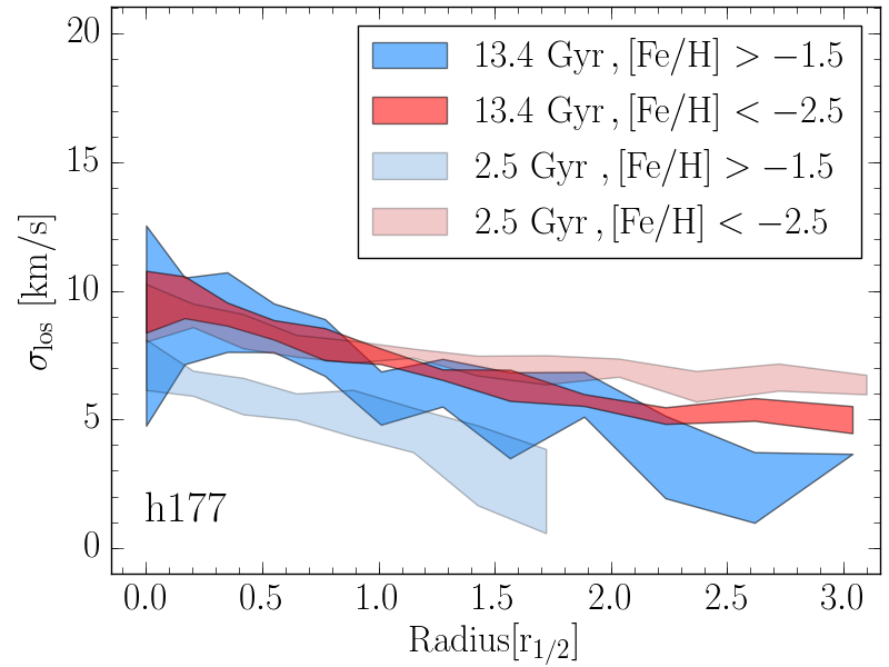
(c) h177 (Sextans)

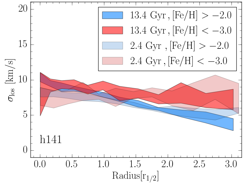
(d) h141 (Ursa Minor)

Figure 12: Line of sight velocity dispersion profile as a function of metallicity of the four models representing the Sculptor, Sextans, Ursa Minor, and Draco dSphs. The velocity dispersion of the metal-rich (in red) and metal-poor stars (in blue) at z=0 is compared to their values at the end of the star formation activity with transparent colours.

As long as star formation is active, gradients are strengthened. This is clearly shown for model h070. It is also seen in cases of residual formation as in model h050 after $t=8\,\rm{Gyr}$ and even for sustained rotating models where the gradient is weaker as in model h021. The link between star formation and gradients is related to the fact that stars form from the gas reservoir in the centre of the galaxies (see Section 3.2). This is illustrated by the stellar age distribution displayed in the second column of Fig. 11. The young and metal-rich stars are essentially located in the galaxy centres, while the older and metal-poor ones are distributed over the entire galaxy. The scatter of the oldest stars arises from the gradually shrinking gas reservoir from which they originate. Indeed the reservoir is dense and spatially extended at early times. Star formation, UV-background and supernovae feedback heating, all result in its depletion and evaporation.

We also note that at given star formation rate and stellar mass, some galaxies end up with a gradient much more pronounced than others. The generation of those types of gradients with strength more than twice as stronger as the others results from their early assembly with faint metal poor galaxies (at about $3\,\rm{Gyr}$) creating a rather extended system with low metallicity stars in the outskirts.

The third and fourth columns of Fig. 11 provide the radial metallicity distribution for our observed comparison sample and their corresponding models. Faint galaxies such as Ursa Minor and Draco, characterized by a star formation that ceased completely $10\,\rm{Gyr}$ ago (Carrera et al., 2002; Aparicio et al., 2001) have marginal gradients (Faria et al., 2007; Kirby et al., 2011; Suda et al., 2017) in agreement with our model predictions. At the other extreme, rotating luminous systems such as NGC 6822 have only weak gradients both in the models and the observations (Kirby et al., 2013). Another clear success is obtained for Andromeda II (Vargas et al., 2014; Ho et al., 2015). Two galaxies appear challenging: both Sculptor and Sextans are lacking metal-rich stars ([Fe/H]$\sim-1.5$) outside their half light radius contrary to our models. The origin of this discrepancy is not fully clear. In the case of Sculptor, we are most likely facing the fact that we only have a limited number of models and even only one for this galaxy for its corresponding metallicity and luminosity. As for Sextans, this failure could be due to the star formation history of the model that is not extended enough compared to the observations (Lee et al., 2009; de Boer et al., 2012a).

3.7 Kinematically distinct stellar populations

Kinematically distinct stellar populations as a function of their metallicity have been mentioned for a number of galaxies, for example Fornax (Battaglia et al., 2006), Sculptor (Tolstoy et al., 2004; Battaglia et al., 2008), and Sextans (Battaglia et al., 2011). The most spectacular example is Sculptor with the metal-poor stars ($\rm{[Fe/H]}<-1.7$) showing a slowly decreasing velocity dispersion with distance to the galaxy centre from $12\,\rm{km/s}$ to $8\,\rm{km/s}$, while its richer counterpart ($\rm{[Fe/H]}>-1.5$) sharply drops to $2\,\rm{km/s}$. In Fornax and Sextans, the difference in velocity dispersion between the most metal-rich population ($\rm{[Fe/H]}>-1.3$, resp. $\rm{[Fe/H]}>-2.2$) and the metal-poor ones is of the order of $2$ to $4\,\rm{km/s}$, less significant than in Sculptor, however still there.

Figure 12 displays the velocity dispersion profiles of models h050 (Andromeda II), h070 (Sculptor), h177 (Sextans) and h141 (Uras Minor). For h070, h177 and h141, we provide the profiles of the metal-rich and metal-poor populations both at $z=0$ and at the end of the star formation. This allows us to assess the impact of the secular dynamical heating. Given the fact that the star formation is still on-going for h050, we only show its profiles at $z=0$. In all cases, younger and more metal-rich stars have the smallest velocity dispersions and radially decreasing profiles. The low velocity dispersion traces that of the cold gas, as discussed in Section 3.2 from which the young stars just emerged. Older stellar populations show rather flat profiles, being kinematically warmer owing to their longer dynamical history. In the most distinct cases, h050 (Andromeda II) and h070 (Sculptor), a difference of about $5\,\rm{km/s}$ is found between the metal-richest and poorest stellar populations, inside $1.5\,\rm{r_{1/2}}$. This difference increases outwards. With shorter star formation histories, the h177 (Sextans), h141 (Ursa Minor) models still show a differential kinematics, however to a lower extent. In all cases, including the cases of sustained star formation such as model h021, the metal-rich stars are systematically warmer than their metal poor counterparts, the difference increasing with radius, in qualitative and quantitative agreement with observations. The secular heating appears to only affects the central regions ($r<r_{1/2}$), increasing their velocities by about $2\,\rm{km/s}$.

Contrary to Benítez-Llambay et al. (2016), in this work we observed no model with sign of late accretion events that could restart the star formation activity, generate gradients, and kinematically distinct stellar populations. Indeed, once being washed out by the UV-background heating, most of our dwarf galaxies evolve as if they were in isolation.

3.8 Open questions and $\Lambda$CDM paradigm

3.8.1 Puzzling cases

Some galaxies, which benefit from detailed observations, fall outside the range of our model predictions. In Section 3.5 we have already mentioned the case of Fornax and Carina. Even more challenging are the properties of the faint, compact, however gas-rich systems, such as Leo T and Leo P, which are seen with residual star formation or at least young stars.

Despite its rather low luminosity ($1.4\times 10^{5}\,\rm{L_{\odot}}$) and velocity dispersion ($\sigma_{\rm{LOS}}\cong 7.5\,\rm{km/s}$) Leo T is embedded in an HI cloud of mass of about $2.8\times 10^{5}\,\rm{M_{\odot}}$ and displays a rather continuous star formation history extending up to a recent past (Weisz et al., 2012). Barely brighter, at the edge of the Local Group, Leo P ($\cong 5\times 10^{5}\,\rm{L_{\odot}}$, Giovanelli et al., 2013; Rhode et al., 2013) is also gas-rich with ongoing star formation (McQuinn et al., 2015). These two galaxies seem to have passed re-ionization without a major decrease of activity. They call for further investigations both of the strength and impact of the UV-background heating and the hydrogen self-shielding.

3.8.2 The stellar mass - halo mass relation: comparison with previous studies

Our simulations predict that Local Group dwarf galaxies with stellar masses larger than $10^{5}\,\rm{M_{\odot}}$ have dark halo virial masses between $2\times 10^{8}$ and $10^{10}\,\rm{M_{\odot}}$. These are at most $3\times 10^{9}\,\rm{M_{\odot}}$ for the classical dwarf spheroidal galaxies with luminosities below $10^{7}\,\rm{M_{\odot}}$.

These predictions are, at given luminosity or stellar mass, somewhat on the low tail of the distribution of dark halo masses found in other studies. Fig. 13 compares the stellar mass $M_{\star}$ vs the halo virial mass $M_{200}$ for different studies. In our simulations, a $10^{5}\,\rm{M_{\odot}}$ stellar mass system has a dark matter halo mass within $[2\times 10^{8}-3\times 10^{9}]\,\rm{M_{\odot}}$. For the same stellar mass, Jeon et al. (2017) find dark haloes in the range $[2\times 10^{9}-4\times 10^{9}]\,\rm{M_{\odot}}$, while in the range $[3\times 10^{9}-8\times 10^{9}]\,\rm{M_{\odot}}$ for the FIRE-2 simulations (Fitts et al., 2017; Hopkins et al., 2017). The values of the APOSTLE simulations (satellite population), not show in Fig. 13 (Sawala et al., 2015) lie in the range $[5\times 10^{8}-6\times 10^{9}]\,\rm{M_{\odot}}$. At higher stellar masses, the divergence is even more pronounced. We predict that a $10^{7}\,\rm{M_{\odot}}$ stellar mass system will be hosted by a dark matter halo within $[2\times 10^{9}-5\times 10^{9}]\,\rm{M_{\odot}}$, while FIRE-2 finds $[8\times 10^{9}-2\times 10^{10}]\,\rm{M_{\odot}}$, the MaGICC simulations (Di Cintio et al., 2014) find $[2\times 10^{10}-3\times 10^{10}]\,\rm{M_{\odot}}$ and the APOSTLE ones $[9\times 10^{9}-10^{10}]\,\rm{M_{\odot}}$, Therefore the difference in predicted dark matter halo masses can reach a factor ten. Before addressing the origin of these differences, it is first important to emphasize that in the context of the the AGORA project (Kim et al., 2016), for the same cooling and feedback implementation, GEAR predicts very similar results compared to other particle-based codes like Gizmo and Gasoline used in the FIRE-2 and MaGICC simulations respectively. The observed differences are thus related to different implementation of physical processes. We discuss in the following what we consider to be the dominant ones: stellar feedback efficiency, strength of the UV-background, hydrogen self-shielding, and the star formation receipts.

The FIRE-2 simulations implement multiple stellar feedback mechanisms (supernovae, OB/AGB mass loss, photo-heating, radiation pressure) with a star formation receipt that let the star form only in very high density regions. These two prescriptions result in a very strong feedback which easily blow out gas in the smallest haloes which becomes dark. Moreover, those simulations use the ionization UV background rates computed by Faucher-Giguère et al. (2009) which is much stronger than the Haardt & Madau (2012) rates we used in our study, for redshifts larger than eight. Consequently, only massive haloes $[\cong 10^{10}]\,\rm{M_{\odot}}$ can retain gas and sustain star formation. In addition to a supernova feedback comparable to our, the MaGICC simulations use early pre-supernova stellar feedback which boost the feedback at early time. These simulations do not include hydrogen self-shielding. In such conditions, as predicted by Okamoto et al. (2008) only massive haloes ($M_{200}\cong 10^{10}\,\rm{M_{\odot}}$) retain their gas during the re-ionization epoch. Faint galaxies produced by Jeon et al. (2017) are at the edge of our predictions. Their shift towards higher halo mass is certainly due to a stellar feedback boosted by core-collapse and pair-instability supernovae.

In our framework, lowering the stellar mass for a given halo mass is possible by boosting the feedback or removing the HI self-shielding, however the stellar line of sight velocity dispersion becomes incompatible with observations, with values too high by about $5\,\rm{km/s}$.

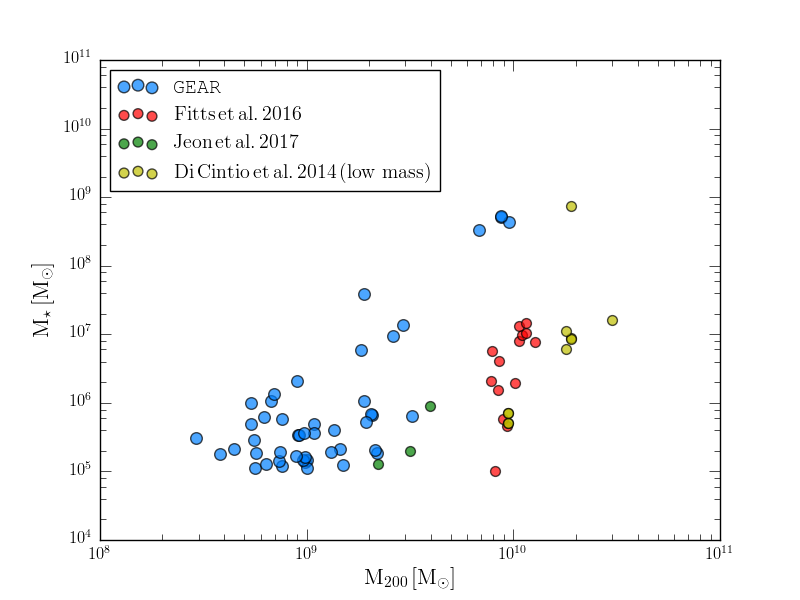
Figure 13: Comparison of the stellar mass $M_{\star}$ vs. the halo virial mass $M_{200}$ between our models in blue and results from other studies based on hydrodynamical codes.

3.8.3 Impact on the missing satellite problem

The question we could raise is whether our small mass dark matter haloes hosting stellar systems are in agreement with the observed number of dwarf satellites around the Milky Way, or in other words, whether we are suffering from a missing satellite problem (Klypin et al., 1999; Moore et al., 1999). Indeed, compared to the above mentioned studies, our models populate the upper edge of the abundance matching predictions (Behroozi et al., 2013), meaning that, at given dark halo mass, they tend to form more stars. However, as discussed in Section 3.3.1, the large scatter in luminosity at given observed velocity dispersion hampers any reliable prediction by this technique.

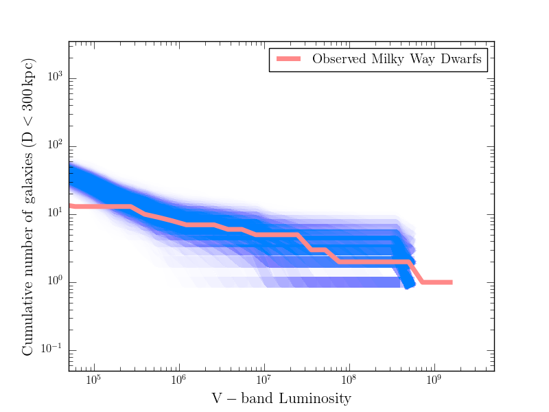
Figure 14: Cumulative number of Milky Way dwarf satellite galaxies within $300\,\rm{kpc}$ as a function of their V-band luminosity. The blue area shows our model predictions, with the observations in red.

To investigate this issue further, we calculated the expected number of dwarf satellites around a Milky Way-like galaxy. Because our cosmological box does not include such a massive galaxy, we used the cumulative number of dark matter haloes of Sawala et al. (2017), inside $300\,\rm{kpc}$. From this distribution, we generated thousand realizations of dark matter haloes. We then assigned to each halo mass a stellar luminosity randomly chosen in the corresponding range of values in our simulations. Fig. 14 displays in blue the resulting cumulative number of dwarfs as a function of their V-band luminosity for each of these thousand models. This prediction is compared to the observations inside the same volume, that is, only considering the Milky Way satellites (red curve). From a luminosity of $10^{5}$ up to $10^{9}\,\rm{L_{\odot}}$ our predictions are in perfect agreement with the observed population. Below $10^{5}\,\rm{L_{v}}$, the cumulative number of galaxies rises steeper than the observed curve. We reserve the study of the regime of the ultra-faint dwarfs for a future study. We note that this agreement above $10^{5}\,\rm{L_{\odot}}$ is obtained naturally and the properties of the dwarfs are also reproduced in detail at $z=0$ with star formation ignited in all haloes more massive than $2\times 10^{8}\,\rm{M_{\odot}}$. This is a major difference with the studies quoted above in which an important fraction of the dark haloes have their star formation totally inhibited by reionization, stellar winds or supernovae feedback. Would dwarf spheroidal galaxies be hosted only in dark haloes more massive than a few $10^{9}\,\rm{M_{\odot}}$ they would exhibit too large a stellar velocity dispersion. This is illustrated by model h039 with a luminosity below $3\times 10^{5}\,\rm{L_{\odot}}$ and a massive dark matter halo of $3\times 10^{9}\,\rm{M_{\odot}}$. Its mean velocity dispersion is $11.7\,\rm{km/s}$ which makes it only marginally compatible with the observed dwarfs at this luminosity.

3.8.4 The cusp/core transformation

Dark matter only simulations predict the density profiles of dark haloes to be universal, independent of the halo mass, with an inner slope of -1 in logarithmic scale (Navarro et al., 1996, 1997). Such cuspy density profiles have been claimed to be in contradiction with the observations, leading to the so called cusp/core problem (Moore, 1994).

Recently, different mechanisms related to the baryonic physics have been proposed to transform a cuspy profile into a core one (Zolotov et al., 2012). In agreement with the theoretical predictions of Pontzen & Governato (2014), simulations from the FIRE project have shown that above a stellar mass of about $10^{6}\,\rm{M_{\odot}}$, a bursty star formation rate generated by a strong stellar feedback transforms a central cusp into a core in the inner one kpc (Oñorbe et al., 2015; Chan et al., 2015; Fitts et al., 2017). A similar trend has been found by Read et al. (2016) in slowly rotating dwarf galaxies. These results are however in contradiction with the APOSTLE simulations of Sawala et al. (2016). The real need of transforming a cusp into a core is indeed still debated. Pineda et al. (2017) discussed that the rotation curves of dwarf galaxies could mimic a core even if the galaxy had a cuspy Navarro, Frenk and White (NFW)’s profile. Strigari et al. (2017) found that, contrary to previous studies (see for example Battaglia et al., 2008), the two kinematically distinct stellar populations in the Sculptor dSph are consistent with populations in equilibrium within a NFW dark matter potential. Very recently, Massari et al. (2018) showed that the internal motions of the Sculptor’s stars are in agreement with a cuspy halo.

To check the effect of baryons in our simulations, we have performed, for each of our zoom-in simulations, a corresponding dark matter only simulation, where all the baryonic mass was transferred into the non-dissipative dark component. A one-to-one comparison between haloes of the two simulations confirms that even after $14\,\rm{Gyrs}$ of evolution, there is no core beyond the gravitational softening scale, for haloes that contains baryons. The halo profiles of the two sets of simulations remain pretty similar even for the most massive systems that continuously formed stars and despite a rather bursty star formation history.

4 Conclusions

We have presented the formation and evolution of dwarf galaxies emerging from a cosmological $\Lambda$CDM framework. We first ran a dark matter only simulation in a $3.4\,\rm{Mpc}$$/h$ box with a resolution of $2\times 512^{3}$ particles. We extracted the 198 haloes which at $z=0$ had virial masses between $4\times 10^{8}\,\rm{M_{\odot}}$$/h$ and $10^{10}\,\rm{M_{\odot}}$$/h$. We selected the 62 haloes whose initial mass distribution was compact enough to allow a zoom-in re-simulation up to $z=0$ with a stellar mass resolution of $1024\,\rm{M_{\odot}}$, including a full treatment of the baryons. From those systems, 27 had a final V-band luminosity larger than $10^{5}\,\rm{L_{\odot}}$, corresponding to Local Group classical spheroidal or irregular dwarfs, and have been studied in detail. These simulations do not include the presence of a massive central galaxy. Nevertheless, they allow us to understand the effect of a complex hierarchical build-up on the final galaxy properties.

We have identified three modes of star formation: quenched, extended and sustained. These modes result from the rate at which the dark matter haloes assemble in combination with the UV-background strength and stellar heating. We have shown that the scaling relations correlating the galaxy integrated properties such as its total V-band luminosity ($L_{\rm{V}}$), central line of sight velocity dispersion ($\sigma_{\rm{LOS}}$), half-light radius ($r_{1/2}$) as well as its gas mass are reproduced over several orders of magnitude.

We have conducted checks in an unprecedented high level of detail. In particular, we could reproduce the properties of six Local Group dwarf galaxies taken as test-beds: NGC 6622, Andromeda II, Sculptor, Sextans, Ursa Minor and Draco. This includes their stellar metallicity distributions and abundance ratios [Mg/Fe], their velocity dispersion profiles, as well as their star formation histories. Metallicity gradients form naturally during the star forming period. Metals accumulate in the centre of the dwarfs where gas and star formation concentrate with time. This mechanism is also at the origin of kinematically distinct stellar populations.

These ensemble of successful results never achieved before by simulations run in a cosmological context, provides further insights onto galaxy formation:

• The observed variety of star formation histories in Local Group dwarfs is intrinsic to the hierarchical formation framework. The interaction with a massive central galaxy could be needed for a handful of cases only, such as the Carina (series of star formation bursts) and Fornax (dominant intermediate age population) dSphs, whose star formation histories are indeed not found in any of our models.

• The inclusion of self-shielding appears to be a major ingredient to allow dark matter haloes with masses as low as $3\times 10^{8}\,\,{M_{\odot}}$ to host stellar systems with dynamical properties in agreement with the observations.

• We confirm the failure of the abundance matching approach at the scale of dwarf galaxies. It is caused by the variety of possible merger histories leading to a large range of final luminosities at given dark matter halo mass, independent of any interaction between the dwarfs and a host massive galaxy.

• Despite the fact that our simulated dwarf galaxies are embedded in haloes with masses standing at the lower boundary of what is found in other works, we do not face any missing satellites problem down to $10^{5}\,\rm{L_{\odot}}$. This is the consequence of an appropriate treatment of the star formation and feedback.

• We do not find evidence for any cusp/core transformation.

• We have uncovered a side effect of the sampling of the dark matter haloes by particles. Even at our high resolution, the discrete representation of the halo leads to a spurious dynamical heating of the stellar component by mutual gravitational interactions. Consequently the galaxy half light radii are artificially increased at $z=0$, particularly in systems in which the star formation has been quenched. However, this sampling could be valid if dark matter were composed of massive black holes. Otherwise the simulations need to reach even higher resolutions to completely avoid this bias.

• While we learn from the successes of the simulations, the challenges are also informative: (i) The existence of faint galaxies ($L_{V}\sim 5\times 10^{5}\,\rm{L_{\odot}}$) with HI and residual star formation, such as Leo T and Leo P, is not predicted in a $\Lambda$CDM framework and a classical UV-background prescription. These cases indicate that further investigation of the strength and impact of the UV-background heating and/or the hydrogen self-shielding is necessary. (ii) While our models match the observations over four dex in luminosity, we have below $10^{6}\,\rm{L_{\odot}}$ a tail of faint dwarfs which stand below the observed range of metallicity. This points to the necessity of an improved treatment of the very first generations of stars.