The Enigmatic (Almost) Dark Galaxy Coma P: The Atomic Interstellar Medium
Abstract
We present new high-resolution HI spectral line imaging of Coma P, the brightest HI source in the system HI 123220. This galaxy with extremely low surface brightness was first identified in the ALFALFA survey as an “(Almost) Dark” object: a clearly extragalactic HI source with no obvious optical counterpart in existing optical survey data (although faint ultraviolet emission was detected in archival GALEX imaging). Using a combination of data from the Westerbork Synthesis Radio Telescope and the Karl G. Jansky Very Large Array, we investigate the HI morphology and kinematics at a variety of physical scales. The HI morphology is irregular, reaching only moderate maxima in mass surface density (peak 10 M⊙ pc-2). Gas of lower surface brightness extends to large radial distances, with the HI diameter measured at 4.00.2 kpc inside the 1 M⊙ pc-2 level. We quantify the relationships between HI gas mass surface density and star formation on timescales of 100-200 Myr as traced by GALEX far ultraviolet emission. While Coma P has regions of dense HI gas reaching the NHI 1021 cm-2 level typically associated with ongoing star formation, it lacks massive star formation as traced by H emission. The HI kinematics are extremely complex: a simple model of a rotating disk cannot describe the HI gas in Coma P. Using spatially resolved position-velocity analysis we identify two nearly perpendicular axes of projected rotation that we interpret as either the collision of two HI disks or a significant infall event. Similarly, three-dimensional modeling of the HI dynamics provides a best fit with two HI components. Coma P is just consistent (within 3 ) with the known MHI – DHI scaling relation. It is either too large for its HI mass, has too low an HI mass for its HI size, or the two HI components artificially extend its HI size. Coma P lies within the empirical scatter at the faint end of the baryonic Tully–Fisher relation, although the complexity of the HI dynamics complicates the interpretation. Along with its large ratio of HI to stellar mass, the collective HI characteristics of Coma P make it unusual among known galaxies in the nearby universe.
1 Introduction
The ALFALFA blind HI extragalactic survey has now produced the largest and most diverse catalog of HI-detected systems ever assembled (Giovanelli et al., 2005; Haynes et al., 2011). The final source catalog contains more than 31,500 extragalactic sources of high significance covering over 7 dex in HI mass. The ALFALFA catalog provides unique perspectives on the population of gas-rich extragalactic sources.
Our group has been actively investigating the physical properties of optically faint galaxies as the ALFALFA catalog has matured and neared completion. These efforts have included both interferometric HI spectral line imaging as well as deep ground-based imaging of selected sources. We have targeted both systems that are candidate Local Group/Volume objects and systems that are almost certainly well outside the Local Group.
This first line of inquiry has led to the characterization of extreme regions of extragalactic parameter space. In the “Survey of HI in Extremely Low-mass Dwarfs” (hereafter “SHIELD”; Cannon et al., 2011a) we are studying those ALFALFA-detected galaxies with HI mass reservoirs smaller than 107.2 M⊙. Using Hubble Space Telescope (HST) imaging, McQuinn et al. (2015a) show that these galaxies are characterized by fluctuating, non-deterministic, and inefficient star formation. The nature of the star formation process in these galaxies is studied in further detail in Teich et al. (2016), where it is shown that stochasticity plays an important role in governing the relationships between recent star formation and neutral hydrogen gas. A companion paper (McNichols et al., 2016) explores the rotational dynamics of these sources, highlighting that galaxies in this mass range probe the transition regime from rotational to pressure support.
This line of inquiry has also led to the ALFALFA discovery of some of the most extreme Local Volume (D 11 Mpc) galaxies known. A series of manuscripts describes Leo P, an extremely low-mass galaxy just outside the Local Group with a single HII region and an extremely low oxygen abundance (Giovanelli et al., 2013; McQuinn et al., 2013, 2015b, 2015c; Rhode et al., 2013; Skillman et al., 2013; Bernstein-Cooper et al., 2014; Warren et al., 2015). Subsequently, the even more metal-deficient Leoncino Dwarf (AGC 198691) was discovered by ALFALFA (Hirschauer et al., 2016).
Moreover, follow-up optical and HI observations have also produced multiple detections of resolved stellar populations in “ultra-compact high velocity clouds” (UCHVCs). These are extended HI systems that have properties such as compact, low-mass halos if they are indeed nearby (within 1-2 Mpc). We refer the reader to Adams et al. (2013, 2015, 2016) and Janesh et al. (2015, 2017) for details about the population of these nearby systems.
The second line of inquiry targets optically faint objects that appear to be outside of the Local Volume. This includes a very small subset of ALFALFA HI detections (1%) that have clear optical counterparts, that have velocities that indicate they are clearly extragalactic, and that are not obviously tidal debris. We have labeled these objects as “(Almost) Dark” galaxies. These enigmatic sources push the boundaries of what might typically be labeled as a “galaxy”; they thus offer unique and powerful insights into the extrema of various fundamental scaling relations.
In Cannon et al. (2015) we presented the basic selection criteria that are used to identify clearly extragalactic (i.e., with recessional velocities sufficient to cleanly separate them from Milky Way HI gas) sources that are (Almost) Dark galaxy candidates. In short, such systems lack an obvious optical counterpart in Sloan Digital Sky Survey (SDSS) imaging (which can be a result of intrinsically low surface brightness or of spatial coincidence) and are unlikely to be tidal in origin. These systems naturally have elevated MHI/LB ratios (Cannon et al. (2015) note that empirically the sources usually have MHI/LB 10). As discussed in Leisman (2017) and Leisman et al. (2017), roughly 1% of the sources in the ALFALFA catalog meet these criteria and are worthy of detailed further exploration to determine their physical properties.
Characterizing these (Almost) Dark galaxies requires intensive follow-up observations, including HI synthesis observations and deep ground-based optical imaging. Previous work by our group has shown that, to date, all of the candidate (Almost) Dark objects turn out to not be truly dark galaxies. Follow-up observations reveal complex tidal systems (Leisman et al., 2016), peculiar sources with large pointing offsets between the ALFALFA and the interferometric centroids (Cannon et al., 2015; Singer et al., 2017), galaxies with low surface brightness similar to ultradiffuse galaxies (Leisman et al., 2017), and sources with other interpretive issues (see Leisman, 2017).
The source that is the focus of this article lies at the intersection of these two efforts. Drawn from the population of more distant (Almost) Dark sources, recent revisions to its distance show that it is actually quite nearby - an extreme Local Volume source that still pushes typical definitions of “galaxy.” This particular source attracted attention as being completely undetected in SDSS, but detected with a signal-to-noise ratio S/N 99 in ALFALFA data products. Examining archival GALEX imaging of the field suggested an optical counterpart. Subsequent detailed HI and optical follow-up observations presented in Janowiecki et al. (2015) revealed a stellar population of extremely low surface brightness stellar population with extended HI gas. This source, AGC 229385, we hereafter will refer to as “Coma P.”
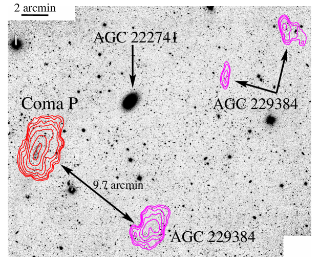
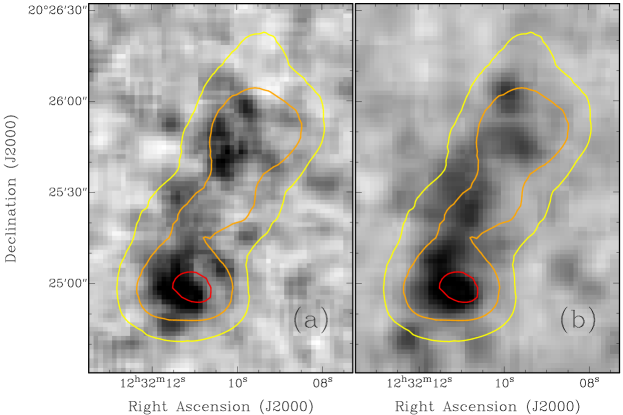
Figure 1 shows the same comparison of the optical and HI morphologies of Coma P as shown in Janowiecki et al. (2015). This galaxy is part of a trio of HI line sources with similar recessional velocities that were identified by ALFALFA and confirmed in the Westerbork Synthesis Radio Telescope (WSRT111The Westerbork Synthesis Radio Telescope is operated by ASTRON, the Netherlands Institute for Radio Astronomy, with support from the Netherlands Foundation for Scientific Research (NWO).) HI images presented in Janowiecki et al. (2015). Very deep optical images acquired with the partially populated One Degree Imager (pODI) on the WIYN222The WIYN Observatory is a joint facility of the University of Wisconsin-Madison, Indiana University, the University of Missouri, and the National Optical Astronomy Observatory. 3.5 m telescope at Kitt Peak Observatory333Kitt Peak National Observatory, National Optical Astronomy Observatory, which is operated by the Association of Universities for Research in Astronomy (AURA) under cooperative agreement with the National Science Foundation. revealed an extended stellar component of low surface brightness associated with the brightest HI source (Coma P). Stellar counterparts of the other two HI sources (AGC 229384 and AGC 229383) remain undetected, with upper limits on the surface brightness of 27.9 and 27.8 mag arcsec-2 in the g′ filter, respectively. These sources have similar systemic velocities to Coma P (VHI 1309 1 km s-1 and 1282 4 km s-1 for AGC 229384 and AGC 229383, respectively) and are offset by 9′7̇ and 15′ from Coma P (see Figure 1). Janowiecki et al. (2015) discuss the physical properties of these sources, based on their adopted distance of 25 Mpc.
Although the recessional velocity of Coma P (VHI 1348 1 km s-1; Janowiecki et al., 2015) and Virgocentric flow model (Masters, 2005) for this region of the sky suggest that it is located well beyond the Virgo Cluster, recent HST images of the source have demonstrated that it is located significantly closer to us. As discussed in detail in S. Brunker et al. (2017, in preparation), the red giant branch of the HST color magnitude diagram is best fit by a distance of only 5.500.28 Mpc. The physical properties of Coma P, which are summarized in Table 1, become increasingly extreme as a result of this change in distance. We note that the HST images do not cover either of the other HI sources that are detected in the ALFALFA and WSRT data as shown in Janowiecki et al. (2015) and Figure 1. While their proximity in both space and velocity strongly suggests association, we do not know whether these objects are at the same distance as Coma P or not.
In this work, we present new HI line synthesis observations of the neutral interstellar medium of Coma P constructed by combining new higher resolution Very Large Array (VLA444The National Radio Astronomy Observatory is a facility of the National Science Foundation operated under cooperative agreement by Associated Universities, Inc.) HI line imaging with the WSRT HI line dataset presented in Janowiecki et al. (2015). The resultant spectral grids are used to study the morphology and dynamics of the HI gas at a variety of angular resolutions. The higher resolution of this new combined dataset allows detailed kinematic and morphological analysis of the HI gas in Coma P, which we present below. We also leverage the spatially resolved nature of the stellar population from the HST images in order to investigate the star formation process in this enigmatic galaxy.
This paper is organized as follows. In § 2 we discuss the HI data handling and combination. § 3 contains detailed discussion about the HI morphology and kinematics. In § 4 we compare the HI properties with those of the stellar populations. The HI dynamics of Coma P are studied and modeled in § 5. We contextualize Coma P in § 6 and summarize our conclusions in § 7.
| Parameter | Value |
|---|---|
| R.A. (J2000) | 12h 32m 10s.3 |
| Decl. (J2000) | 20°25′23″ |
| Adopted distance (Mpc) | 5.50 0.28aaS. Brunker et al. (2017, in preparation) |
| MB (mag) | 10.710.14aaS. Brunker et al. (2017, in preparation) |
| M⋆ (M⊙) | (1.00.3) 106aaS. Brunker et al. (2017, in preparation) |
| MHI (M⊙) | (3.48 0.35) 107bbUsing SHI 4.87 0.04 Jy km s-1 from Haynes et al. (2011). |
| DHI (kpc)ccMeasured at the 1 M⊙ pc-2 level. | 4.00.2 |
| SFRFUV (M⊙ yr-1) | (3.11.8) 10-4 |
2 Observations and Data Handling
2.1 HI Data Products
We use the same WSRT data products as those presented in Janowiecki et al. (2015), to which we refer the reader for details of the data handling. Briefly, three separate 12 hr synthesis tracks were obtained for program R13B/001 (P.I. Adams). A 10 MHz wide band is separated into 1024 channels, delivering a native spectral resolution of 2.06 km s-1 ch-1. Following manual excision of radio-frequency interference and bad data, the bandpass shape was removed using observations of the primary calibrator. The data were then self-calibrated using a continuum image of the target field.
VLA HI spectral line imaging of Coma P was obtained in 2015 February and March for program VLA/15A-307 (P.I. Leisman). A total of 8 hr of observing time was acquired in the “B” configuration of the array (maximum and minimum baseline lengths of 53 and 1 k at 21 cm, nominal beam size 6″). The primary calibrator was 3C286 and the phase calibrator was J11582450. Observational overheads resulted in a total of 6.3 hr of on-source integration time. Reduction of the VLA data followed standard practices within the environment of the Common Astronomy Software Application (CASA555https://casa.nrao.edu/; McMullin et al., 2007).
2.2 Combination Imaging
In order to leverage both the surface brightness sensitivity of the WSRT data and the angular resolution of the VLA data, we use both sets of calibrated visibilities to create three-dimensional data cubes of HI line emission. While the combination of single-dish and interferometric data is common (the so-called “zero-spacing correction”), the combination of datasets from different interferometric observatories is less frequently employed. In addition to the different synthesized beam shapes of the individual observatories, they also typically employ different weighting schemes for calibrated visibilities. We refer the reader to Carignan & Purton (1998) for an early discussion of techniques.
There are effectively two strategies for the combination of interferometric datasets. In the first, appropriately weighted visibilities are combined in the image plane (e.g., Sorgho et al., 2017). In the second, the visibilities are weighted, combined in the plane, and imaged by deconvolving with a beam that combines the shape of the beams for the input datasets (e.g., Bernstein-Cooper et al., 2014). We favor the second strategy for image combination, since the CASA CLEAN algorithm is specifically designed to be able to image multiple datasets on the fly.
The relative weights of the individual data sets were calculated by measuring the rms as a function of time and of baseline in line-free channels using the CASA task statwt. We then performed rigorous checking for matching HI fluxes per channel between datasets by imaging the individual, calibrated databases separately and by enforcing appropriate tapering in the domain to achieve similar beam sizes. As expected, the full-resolution VLA images recover less flux than the WSRT images, and both recover less than the ALFALFA flux (see below). After tapering to common resolutions we find agreement between the fluxes per channel in all datasets.
| Data Product | Beam Size | rms | Peak NHIaaHI column density as defined assumes a uniform source that fills the beam, so it should always increase with
increasing angular resolution if there is structure. |
SHI |
|---|---|---|---|---|
| (mJy Bm-1) | ( cm-2) | (Jy km s-1) | ||
| VLA data only | 690 496 | 0.77 | 17.25 | 3.02 0.30 |
| Combined data, High resolution | 75 75 | 0.69 | 12.8 | 2.92 0.29 |
| Combined data, Medium resolution | 125 125 | 0.56 | 9.3 | 2.96 0.30 |
| Combined data, Low resolution | 17″ 17″ | 0.66 | 8.5 | 3.56 0.36 |
| WSRT data only | 625 178 | 0.58 | 5.89 | 4.43 0.44 bbJanowiecki et al. (2015) |

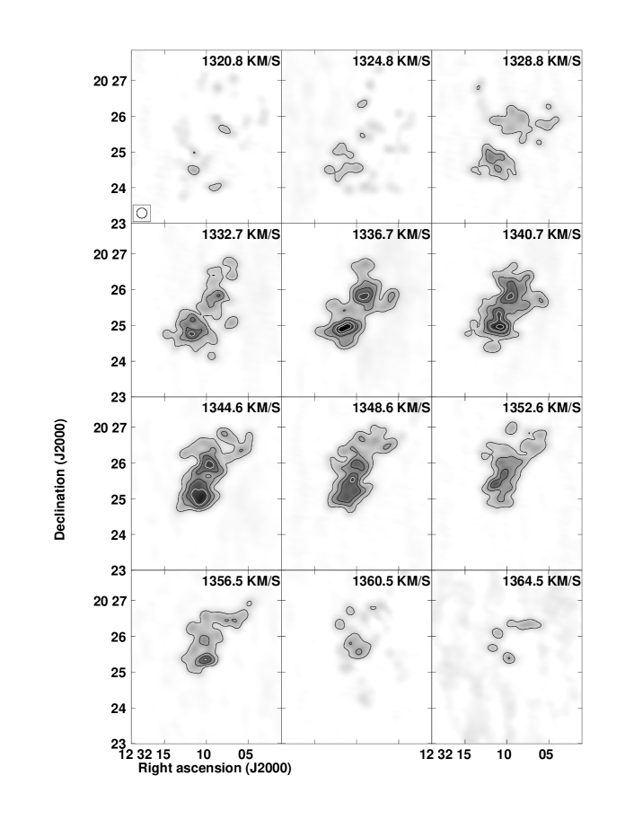
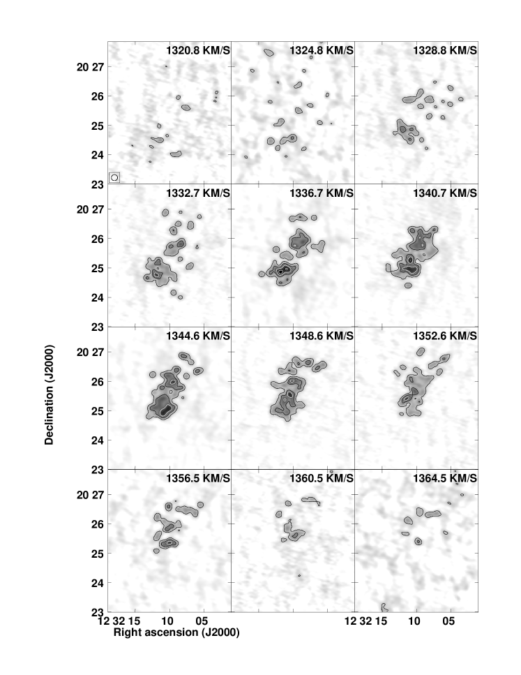
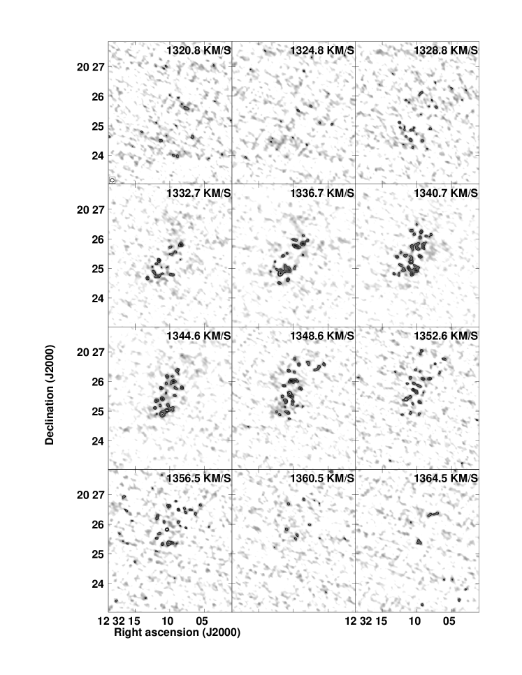
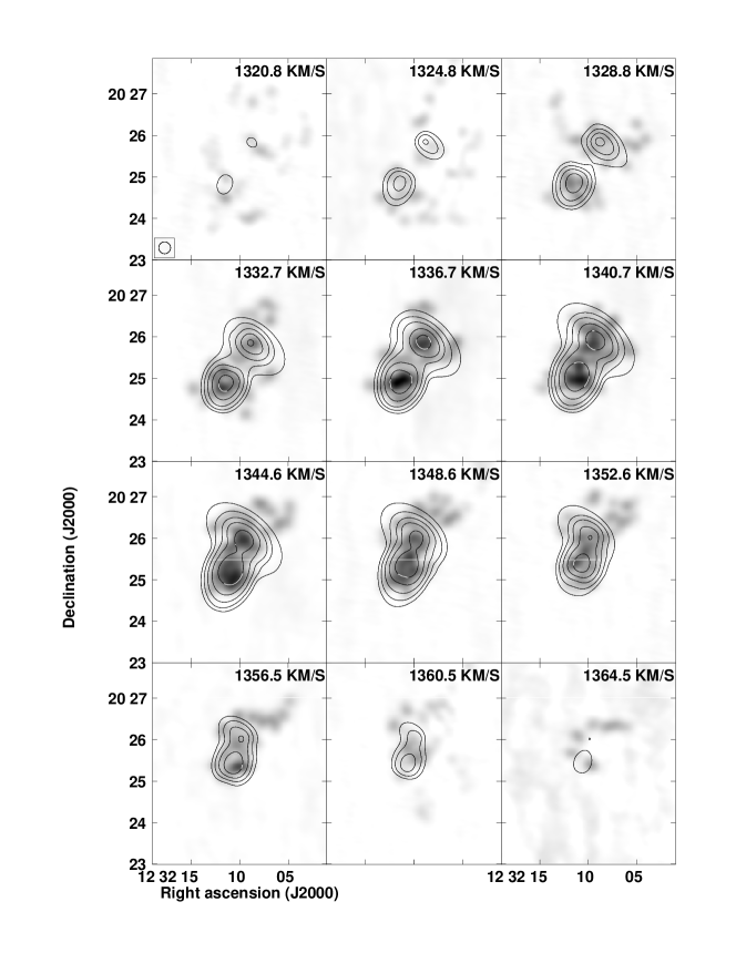
With the individual databases appropriately weighted, we then imaged all of them simultaneously in the CASA CLEAN algorithm. We employ the “Briggs” weighting scheme and vary the “robust” weighting parameter (which ranges from 2 to 2 for uniform to natural weighting) and the -domain tapering to produce final cubes at high, medium, and low angular resolutions. Table 2 summarizes basic parameters of each final dataset. The final data cubes were produced using interactive clean boxes and were cleaned to the 0.5 level (determined in line-free channels of cubes with very small numbers of clean iterations). Residual flux rescaling was employed on each resulting cube following Jörsäter & van Moorsel (1995). We present the HI data cubes at low, medium, and high resolution in channel map format in Figures 2, 3, 4, respectively.
Each resulting data cube was threshold-blanked at the 2 level and then closely examined by hand for spectral and spatial continuity of features. The global HI line emission in these blanked cubes is plotted in Figure 5. The systemic velocity of Coma P in each cube is assigned to the intensity-weighted mean. The resulting blanked data cubes were then collapsed to create two-dimensional images of HI mass surface density, HI intensity-weighted velocity, and HI intensity-weighted velocity dispersion. Note by examining Table 2 that the integrated HI flux from Coma P increases as the angular resolution decreases, and that the products with the lowest angular resolution (WSRT data only, highest surface brightness sensitivity) recover SHI = 4.43 0.44 Jy km s-1. This agrees with the ALFALFA HI flux integral (SHI 4.87 0.04 Jy km s-1) within errors.
3 The HI Content of Coma P
Our combined VLAWSRT images reveal the properties of the HI gas in Coma P in unprecedented detail. Our low-resolution images are in excellent agreement with those presented in Janowiecki et al. (2015). We refer the reader to that work for a discussion of the gas with extended low surface brightness in Coma P, as well for details about the other HI line sources that are in close angular and velocity proximity.
3.1 HI Morphology
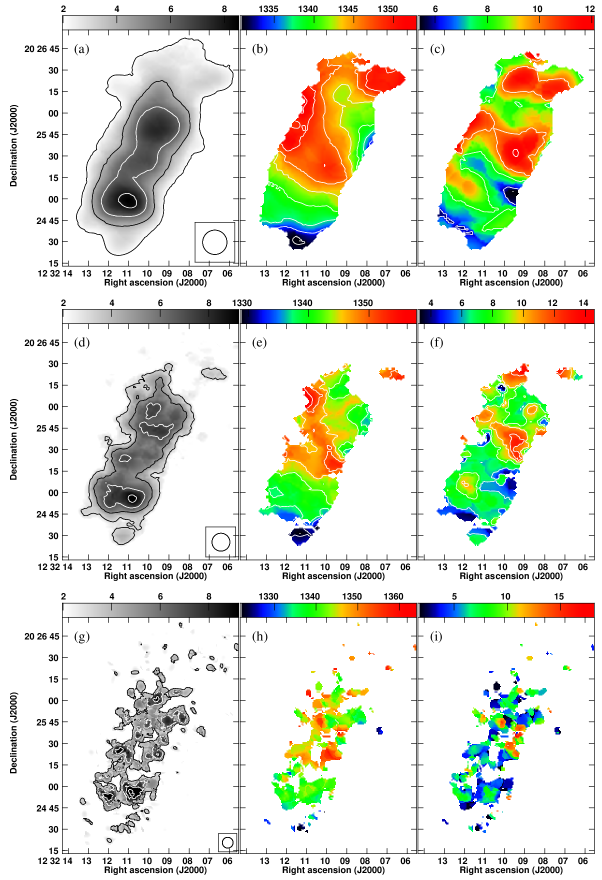
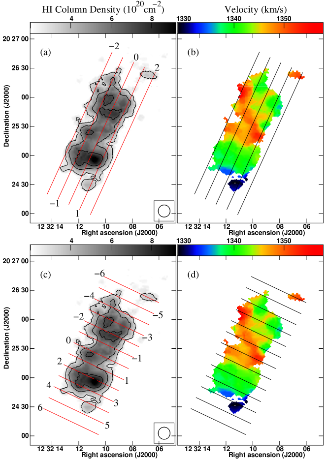
In Figure 6 we show two-dimensional representations of the HI column density (calibrated in units of 1020 cm-2), the intensity-weighted HI velocity, and the intensity weighted HI velocity dispersion. Each of these images is shown at low (17″ beam), medium (125 beam), and high (75 beam) angular resolutions. The corresponding elements of physical resolution are 453 pc, 333 pc, and 200 pc, respectively, assuming the distance of 5.5 Mpc from S. Brunker et al. (2017, in preparation).
In panels (a), (d), and (g) of Figure 6, the HI column density distributions are shown in grayscale and with uniformly spaced overlying contours. At 450 pc resolution the HI is smoothly distributed along an axis running roughly southeast to northwest, while HI gas of lower surface brightness extends beyond the outermost contour shown. The overall HI morphology at low angular resolution agrees well with the WSRT-only images as presented in Janowiecki et al. (2015).
At low and medium resolutions, the HI morphology is highlighted by moderate HI mass surface densities throughout most of the galaxy. At low (Figure 6a) and medium (Figure 6d) angular resolutions, HI columns exceed NHI 5 1020 cm-2 (4.0 M⊙ pc-2). Two maxima in HI column density are located on either end of the HI distribution. The densest HI gas (NHI 9 1020 cm-2 or 7.2 M⊙ pc-2) is located in the southeastern end of the HI distribution, while the secondary HI maximum peaks at only slightly lower HI column densities. In between these maxima is the morphological centroid of the HI gas, where the HI column densities are slightly lower.
At 200 pc resolution (Figure 6g) we resolve only the highest peaks in mass surface density in the HI gas. Interestingly, the HI maxima seen in the lower resolution images resolve into multiple individual HI peaks. At a few locations the HI column density exceeds the “canonical” threshold of NHI 1021 cm-2 that was empirically associated with ongoing star formation in dwarf irregular galaxies (Skillman, 1987). The southeastern HI maximum seen at low and medium resolutions achieves the highest HI mass surface density in the entire galaxy (NHI 1.28 102 cm-21 or 10.3 M⊙ pc-2).
As we discuss in detail below, the HI gas in Coma P is more complicated than a simple thin disk such as those found in many other dwarf galaxies. With this caveat in mind, we define the morphological center of Coma P by examining the medium-resolution HI data. Using the 3 1020 cm-2 contour as a guide, we find that an ellipse with an axial ratio of 2.1:1, oriented along a major axis rotated 155° east of north, provides a suitable representation of the HI morphology at this surface density level. The HI centroid derived using this approach is (,) = (12h32m10s.3, 20°25′23′′). The corresponding inclination is 63°, which agrees with the 6°34°derived by Janowiecki et al. (2015).
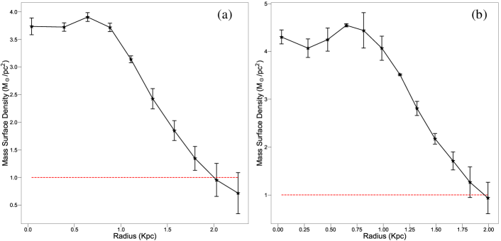
The HI distribution is resolved along both the major and minor axes. We thus use the parameters derived above to create the radial profiles of the HI gas in Coma P that we present in Figure 7. These profiles (created using the ELLINT task in the GIPSY666The Groningen Image Processing System (GIPSY) is distributed by the Kapteyn Astronomical Institute, Groningen, Netherlands. software package; van der Hulst et al., 1992) are explicitly corrected for beam smearing using the Gaussian approximation discussed in Wang et al. (2016). Specifically, the corrected and uncorrected HI sizes (DHI and DHI,0, respectively) are related to the lengths of the major and minor axes of the beam (Bmaj and Bmin, respectively) via . Beam smearing is negligible when the observed HI size is much larger than the angular size of the beam; this is the case for our HI observations of Coma P.
The radial profiles allow us to quantify both the HI size and the HI scale length of Coma P. The average (radially integrated) HI mass surface density in the inner region is nearly flat within errors at a value of 4.25 M⊙ pc-2 (at 125 resolution). There is a small increase in mass surface density at 0.75 kpc in both profiles, corresponding to where the radial integration passes through both the primary and the secondary HI maxima. Moving outward the profile falls off smoothly. The horizontal dotted lines in Figure 7 demonstrate that the HI diameter is 4.00.2 kpc measured at the 1 M⊙ pc-2 level. The HI scale length of Coma P is measured by fitting an exponential function to the six data points at radii larger than 1 kpc in the low-resolution radial profile (Figure 7(b)). We find a scale length of 0.8 0.1 kpc, where the uncertainty is estimated by including and then excluding the next inner radial profile point in the exponential fit.
3.2 HI Kinematics
The HI kinematics of Coma P are extremely complex. The intensity-weighted HI velocity fields presented in panels (b), (e), and (h) of Figure 6 do not show the signatures of coherent, solid-body rotation that are typical of low-mass galaxies (e.g., Oh et al., 2015). Rather, Coma P has multiple velocity gradients within the HI distribution, along different position angles. For example, at low resolution, in the southern region of the galaxy there is a smooth velocity gradient spanning 20 km s-1 oriented along the HI major axis. In the central region of the HI distribution, gas at the highest recessional velocity spans the entire minor-axis diameter of the galaxy. Moving northward, the isovelocity contours become nearly perpendicular to those in the southern region. A simple scenario of a smoothly rotating disk is insufficient to describe the global kinematics. This conclusion was already evident in the WSRT data as presented by Janowiecki et al. (2015). We note that our low-resolution velocity field is consistent with the one shown in that work.
The images with higher angular resolution show similar kinematic signatures to those seen in the low-resolution velocity field. At 333 pc resolution (Figure 6(e)), the southern velocity gradient and the changing orientations of the isovelocity contours in the north are still present. The lower surface brightness sensitivity of these images results in some noticeable changes, especially in the north and central regions. At the highest angular resolution we again are sensitive to only the densest parcels of gas. Thus for clarity we do not overlay isovelocity contours on Figure 6(h). The signatures of extremely complicated HI gas kinematics remain prominent at all angular resolutions.
The intensity-weighted velocity dispersion images of Coma P are shown in panels (c), (f), and (i) of Figure 6. At low angular resolution the magnitudes of the HI velocity dispersion range from 6 to 12 km s-1, typical of the values found in low-mass galaxies (e.g., McNichols et al., 2016). In the southern region of the galaxy (where the nominal smooth velocity gradient was identified in the discussion above) the velocity dispersions remain below 10 km s-1. In the center of the HI distribution the values increase to 12 km s-1, corresponding to the onset of the changes in directions of the isovelocity contours.
Moving to the medium- and high-resolution images shown in panels (f) and (i) of Figure 6, the same signatures remain: lower velocity dispersions are found in the south, with a significant increase toward the north. Interestingly, the northern and southern maxima in HI mass surface density have very different dispersion characteristics. The gas with higher mass surface density in the south is characterized by low dispersion gas (v 8 km s-1), with a small increase to 10 km s-1 on the far eastern portion of the HI maximum. In contrast, the northern HI peak (which contains sub-structure at 125 resolution) contains the region of the galaxy with gas of the highest dispersion (v 14 km s-1).
It is important to note that the collapse of a three-dimensional datacube into a two-dimensional image loses information as a result of the weighting by intensity per pixel. A comparison of Figure 6 with the channel maps shown in Figures 2, 3, and 4 demonstrates this by the difference in velocity ranges between the two- and the three-dimensional products. Given the kinematic complexity of Coma P, we therefore explore the full three-dimensional data products in § 5 below.
4 HI and Star Formation in Coma P
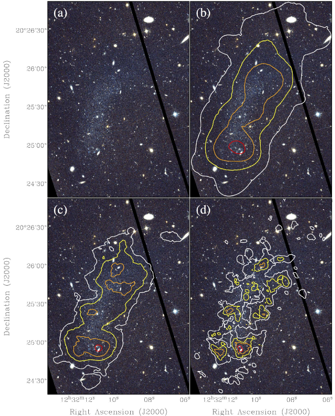
To understand the relationship of the HI gas to the underlying stellar populations in Coma P, in Figure 8 we overlay the same sets of HI column density contours as shown in panels (a), (d), and (g) of Figure 6 on a color HST image (created using the F606W filter image as blue, the F814W filter as red, and a linear average of the two filters as green; see S. Brunker et al. 2017, in preparation). Figure 8(a) shows the same HST color image as in S. Brunker et al. (2017, in preparation), with no HI contours so as to allow detailed inspection of the stellar population and to identify foreground stars and background galaxies. As described in detail in Janowiecki et al. (2015) and S. Brunker et al. (2017, in preparation), the stellar population of Coma P has a remarkably low surface brightness (peak surface brightnesses in the g′, r′, and i′ bands of 26.40.1 mag arcsec-2, 26.50.1 mag arcsec-2, and 26.10.1 mag arcsec-2, respectively). With a morphology similar to that of the HI images shown in Figure 6, the stellar population arcs from southeast to northwest. Nearly all of the compact and luminous sources seen in this field are foreground stars or background galaxies. The individual stars in Coma P are faint but spatially resolved, resulting in the diffuse distribution of stars that is contained within the HI contours. A few stellar clusters are apparent, and these are discussed in further detail below.
In panels (b)-(d) of Figure 8, the HI contours as shown in Figure 6 are color-coded for ease of interpretation. Comparing the low- and medium-resolution HI contours to the HST images, we find excellent spatial agreement between the HI gas of high column density and the locations of the faint but resolved stars in Coma P. Effectively all of the stellar population of Coma P is located within HI gas with NHI 5 1020 cm-2 (4.0 M⊙ pc-2). The highest HI mass surface densities in the southeastern region of the galaxy are cospatial with what appear to be individual stellar clusters or extended star formation regions.
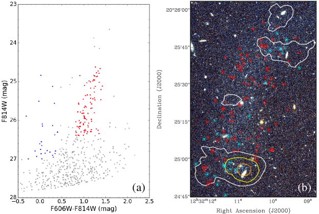
To further investigate the relationship between the HI gas and the resolved stars in Coma P, Figure 9 shows the locations of individual red and blue stars on the HST color image. Panel (a) shows the color-magnitude diagram as presented in S. Brunker et al. (2017, in preparation). Therein, blue and red stars are color-coded. Blue stars are selected as having F814W magnitudes brighter than 27.0 and F606WF814W colors bluer than 0.4, while red stars are the individual red giants used for the distance determination as discussed in S. Brunker et al. (2017, in preparation). These red and blue stars are then plotted on the color HST image in panel (b) as cyan and red asterisks. HI column density contours from the medium-resolution (125 beam) image are shown at levels of (7, 8, 9) 1020 cm-2. As expected for an old stellar population that is well mixed, the red stars are uniformly distributed across the galaxy. In contrast, the blue stars are decidedly concentrated within the regions of highest HI mass surface density.
As discussed in detail in Janowiecki et al. (2015), the star formation properties of Coma P are extreme. The source is not detected in deep ground-based H imaging, implying that the current rate of massive star formation is zero. Curiously, Coma P is detected by GALEX in both the near-UV (NUV) and far-UV (FUV) bands (although at low S/N). We compare the low-resolution HI image with the GALEX FUV and NUV images in Figure 10. The ultraviolet emission detected by GALEX is cospatial with the HI gas detected in Coma P. By comparison with the HST images in Figure 8 it is evident that the flux from the resolved stellar populations is dominated by stars that are capable of producing UV photons but not of photoionizing HII regions (S. Brunker et al. 2017, in preparation). Note that the southern maximum in HI column density is cospatial with the maxima in both GALEX images. This is the same location identified above in the HST images as harboring stellar clusters. We note, however, that there is also a significant background spiral galaxy nearby that makes this interpretation difficult (see the highest HI contour in Figure 8(c) and in both panels of Figure 10).
We estimate the FUV-based star formation rate using the calibration derived from resolved stars in McQuinn et al. (2015b). The resulting global far-ultraviolet star formation rate is very low: SFRFUV (3.11.8) 10-4 M⊙ yr-1. This is equal to the lowest far-ultraviolet star formation rate amongst the galaxies in the SHIELD sample (Teich et al., 2016). However, the FUV flux in Coma P is extended over a much larger area than in the (physically smaller) SHIELD galaxies. A spatially resolved analysis of the FUV star formation rate density versus the HI mass surface density (e.g., as presented in Teich et al., 2016) is not possible at the low S/N ratio of the GALEX FUV images. Deeper UV imaging of Coma P would be especially useful for studying the star formation on timescales of 100-200 Myr.
5 The Complicated HI Dynamics of Coma P
As discussed in § 3.2, the HI kinematics of Coma P are not amenable to standard modeling techniques. The two- and three-dimensional data products (see Figures 2, 3, 4, 6) demonstrate this clearly. In an effort to understand the complex neutral gas dynamics of Coma P, we thus perform two types of analysis on the three-dimensional datacubes.
5.1 Spatially Resolved Position-Velocity Analysis
In the first line of investigation we apply the spatially resolved position velocity analysis developed in Cannon et al. (2011b) and employed in McNichols et al. (2016) and Cannon et al. (2016). This technique allows us to estimate the projected rotation velocity of a source when its kinematics are not well described by a simple tilted ring. The approach relies on identifying a projected HI major axis, which is typically that axis along which the largest velocity gradient is present. In some cases this HI major axis aligns with the major axis of the stellar component. However, this is not necessarily the case for all dwarf galaxies, especially for those systems with extremely unusual gas kinematics (see application of the approach to the post-starburst galaxy DDO 165 in Cannon et al., 2011b). The HI minor axis is assumed to be offset from the major axis by 90°.
The spatially resolved position analysis then examines a collection of position-velocity slices for the major and minor axes. Each slice is the width of, and is offset from the neighboring slice by, the HI beam width. The series of major and minor axis slices allow the identification of the largest projected rotation velocity, both along the major axis and also as a change in velocity of the HI centroids of the minor axis slices. Further, this approach allows us to isolate kinematically distinct features (e.g., Cannon et al., 2011b) in the gas.
To balance angular resolution with sensitivity, in this analysis we examine the medium-resolution (125 beam) data cube (see Figure 3). We identify the HI major axis interactively by examining position velocity slices at a range of position angles. The resulting major axis is oriented at a position angle of 335° measured east of north. This angle is in agreement with the direction of the maximum projected velocity gradient in the moment one images at both low and medium resolutions (see Figure 6), and it is also in rough agreement with the position angle of the stellar component (see Figure 1). The HI minor axis is 90° away (at 65°), again rotated east through north. The HI dynamical center is assumed to be cospatial with the adopted morphological center (see discussion in § 3.1): (,) = (12h32m10s.3, 20°25′23′′). Note that since the slices are the width of the HI beam, the absolute position of the dynamical center is not critical for interpretation.
Based on the 125 (333 pc) beam, we then symmetrically slice (i.e., use the same number of slices at positive and negative angular offsets from the major and minor axes) the data cube along both the major and the minor axes as shown in Figure 11. Five major axis slices are required to cover the HI distribution of Coma P, while 13 minor axis slices are required. Such an axial ratio is expected based on the inclination derived above. On both the major and the minor axes, the central slice is numbered “0.” For the major axis slices, those with negative numbers are located east of the central slice and those with positive numbers are located west of the central slice. Likewise, for the minor axis slices, those with negative numbers are located north of the central slice and those with positive numbers are located south of it.
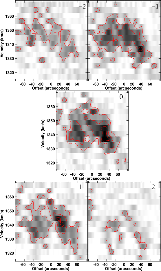
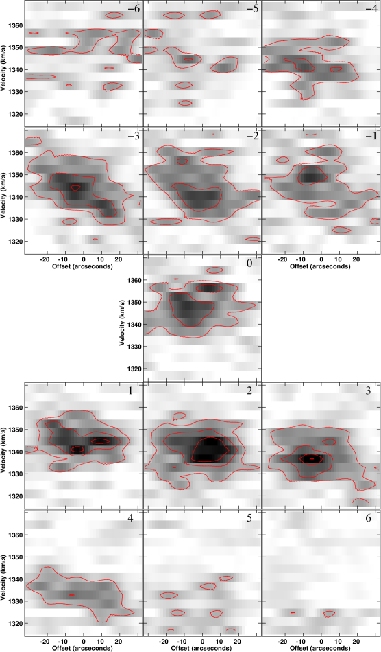
The resulting spatially resolved position-velocity slices for the major and minor axes are presented in Figures 12 and 13, respectively. In each figure the axes and color scalings are identical. Contours are overlaid at the 3, 6, 9, and 12 levels in each panel. These figures contain a wealth of information about the kinematics of the HI gas in Coma P.
Beginning with the major axis slices shown in Figure 12, all slices show two opposing velocity gradients: a crescent-shaped structure in the plane of velocity versus offset, the shape and dynamic range of which are the same as shown in Janowiecki et al. (2015). This signature of two opposing velocity gradients is most easily interpreted as two separate velocity components within the HI distribution of Coma P. Moving from the central slice to either positive or negative offset reveals that the HI velocity structure on the major axis does not change as a function of offset from the center. This confirms the identification of the major axis of one of the HI components. Further, it demonstrates that the turnover in velocity as a function of offset, likely caused by the presence of a second HI kinematic component, extends throughout the entire HI distribution of Coma P.
The minor axis slices confirm the interpretation of two kinematic components in the HI gas. The HI velocity structure along the minor axis does indeed show a moving velocity centroid from one side of the galaxy to the center (e.g., examine the highest S/N contours in the series of slices with negative numbers). However, importantly, around the central slice this signature turns over in velocity space and then continues in the opposite direction on the other side of the galaxy (examine the highest S/N contours in the series of slices with positive numbers). Such a turnover in velocity space is very unusual. A galaxy with normal HI kinematics (that are well described by a simple tilted ring model) would show the signature of changing centroid position across all of the minor axis cuts. Note that even if the inclination were in fact very low (unlikely for Coma P based on the optical and HI morphologies) and the signature of projected rotation very subtle, it would still not result in a turnover in velocity space as a function of position.
Using the spatially resolved position velocity analysis as a guide, we can coarsely separate the two HI gas components in the observed low- and medium-resolution datacubes. We stress that this separation is not clean, either spatially or spectrally. HI gas connects these two kinematic components in the data cubes and in the position velocity slices through them. With this caveat in mind, we estimate that the relative HI mass ratio of the two HI components is in the range of (0.6:1) to (0.8:1); varying the masking and threshold levels used to identify the two components changes the resulting mass ratio. While the absolute value of the mass ratio is uncertain, the masses of the two components are of the same order.
It is difficult to interpret the velocity gradients seen in the position velocity slices of Figures 12 and 13 as coherent rotation. If we take the projected velocity gradients at face value, then we can make coarse estimates of the dynamical masses of the two kinematic components. We use the turnover in projected velocity along the central major axis slice as the boundary between the two components. The more massive component (extending to positive angular offsets in Figure 12) has a maximum observed projected velocity gradient of 35 10 km s-1 that spans 60″. Likewise, the less massive component also spans an angular offset of 60″ with a maximum observed projected velocity gradient of 30 10 km s-1. If we interpret each of these maximum projected velocity gradients as the signature of rotation of each kinematic component, then the inclination-corrected rotational velocities of the more and less massive components are 20 10 km s-1 and 17 10 km s-1, respectively; each subtends 800 pc (30″). We stress that this interpretation is highly uncertain, since the dynamics of Coma P are certainly a mixture of rotation and of non-circular motions.
Using the estimates of angular offset and rotational velocity above, a simple estimate of the dynamical masses (Mdyn ) of the two kinematic components of Coma P results in Mdyn 7.2 107 M⊙ and 5.3 107 M⊙. We conservatively estimate a 50% uncertainty to highlight the aforementioned difficulties in determining the physical properties of Coma P. Correcting the HI gas mass by a factor of 1.35 for helium, metals and molecules, and assuming M⋆ (1.00.3) 106 M⊙ (see S. Brunker et al. 2017, in preparation), we find a total baryonic mass Mbary 4.8 107 M⊙. Summing the dynamical masses of the two components (Mdyn 1.2 108 M⊙) within the extent of the HI shows that Coma P is dominated by dark matter at the level of roughly 2.5 to one.
5.2 Three-Dimensional Modeling of the HI Distribution

The second line of investigation attempts to fit a three-dimensional model to the HI data cube using the “Tilted Ring Fitting Code” (“TiRiFiC”) software package (Józsa et al., 2007). By working with the full three-dimensional data cube, TiRiFiC eliminates the loss of information when using only the velocity field for tilted ring fitting. Further, TiRiFiC allows for modeling of multiple HI disks and for inhomogeneities in the surface brightness distribution. In situations where complicated gas kinematics are present (as in Coma P), this allows a direct comparison of the resulting model with the observed data cube.
The TiRiFiC package was used in interactive mode to fit the medium-resolution (125 beam) data cube. The resulting best-fit models contain two HI components: a more massive component (located in the southeastern region of the galaxy) and a less massive segment that is undergoing either infall or outflow and is moving with respect to the center of the galaxy. No simple model with a single inclined disk was able to accurately describe the HI kinematics of Coma P.
Figures 14 and 15 present this best-fit model as contours overlaid on the same low-resolution and medium-resolution channel maps as shown in Figures 2 and Figures 3, respectively. The model reproduces the complicated three-dimensional gas distribution and kinematics very well. Moving from low to high velocities, one can easily differentiate the two HI components, both spatially and spectrally. The opposing velocity gradients of the two components are also clearly visible. The two model kinematic components have a relative mass ratio of 0.64: 1, with the more massive component in the southeastern region of the disk. This compares favorably with the HI and dynamical mass ratios of the two components estimated in § 5.1.
The interpretation of the best-fit model from TiRiFiC is very similar to the interpretation of the spatially resolved position velocity slices discussed above. Specifically, the best-fit model contains two kinematically distinct HI components. The kinematic discontinuity in the central region of the galaxy (highest velocity gas in Figures 14 and 15) is the result of the presence of two HI components of differing masses. Whether this event is best described by two low-mass galaxy disks or by the infall of HI gas into Coma P is not certain. Given the current and recent quiescence of the galaxy in terms of star formation rate (see discussion above and in S. Brunker et al. 2017, in preparation), it is unlikely that the kinematics are described as an outflow driven by star-formation. The extended gas of low surface brightness would then be the result of this ongoing interaction or infall event.
6 Contextualizing Coma P
Various observed properties of Coma P make it an extremely unusual dwarf galaxy when compared to other objects in the Local Volume. The proximity of the galaxy is unusual given its large recessional velocity. The source is currently quiescent in terms of massive star formation but yet has significant UV flux indicative of star formation on timescales of 100-200 Myr. The optical surface brightness is extremely low, and the HI properties are unusual for a low-mass halo. We now attempt to contextualize Coma P with respect to other Local Volume galaxies.
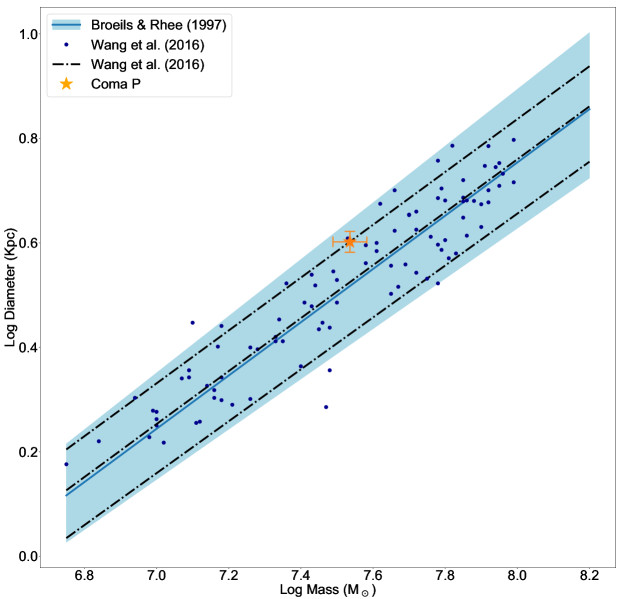
Comparing Coma P to the low-mass galaxies in the SHIELD sample (Cannon et al., 2011a; McNichols et al., 2016; Teich et al., 2016), Coma P is slightly more HI-massive than all but one of these galaxies. Given this HI mass, Coma P is large in physical size. As discussed in § 3.1, the HI diameter is measured to be 4.0 0.2 kpc at the 1 M⊙ pc-2 level. This allows us to place Coma P on the MHI–DHI relation–the empirical relationship between HI size and total HI mass (see first characterization in Broeils & Rhee, 1997). While the origins of this relation are likely multi-faceted, Wang et al. (2016) use data for hundreds of nearby galaxies to show that the relationship is linear over four orders of magnitude in HI mass (7 log(MHI/M⊙) 11). The relation appears to continue to lower masses, although the small number of sources makes this extension uncertain at the present time.
In Figure 16 we show the MHI–DHI relation including Coma P and a subset of the data from the sample of Wang et al. (2016). Coma P is just consistent with the 3 fit derived by Wang et al. (2016) (note that the parameterizations of the MHI–DHI relation by Broeils & Rhee (1997) and Wang et al. (2016) are effectively identical). The galaxy can be considered to have a large HI distribution given its HI mass, a smaller total HI mass given its physical size, or an artificially extended HI size due to the presence of two HI components.
It is important to stress that the MHI–DHI relation is meaningful for isolated galaxy disks where the physical size of the HI component is directly related to the gravitational potential of the parent halo. A complicated system such as Coma P, where the HI kinematics favor a model with multiple HI components, may not be appropriately interpreted in the context of the MHI–DHI relation. With this caveat in mind, taken at face value, the HI is considerably extended in Coma P compared to expectations based on the total HI mass of the system.
In addition to the large HI size of Coma P, its total HI mass is large compared to its stellar mass. Janowiecki et al. (2015) estimate a very large MHI/M⋆ ratio using stellar masses derived from standard mass-to-light scaling relations. While MHI/M⋆ is independent of distance, S. Brunker et al. (2017, in preparation) suggest a significantly revised stellar mass from HST imaging of M⋆ (1.00.3)106 M⊙. Regardless of the exact value of M⋆, Coma P is one of the most HI-rich galaxies known relative to its stellar mass, especially among sources with accurately measured MHI/M⋆. The estimated change in stellar mass moves Coma P within the scatter of the sources with stellar masses near 106 M⊙ in Huang et al. (2012) and Janowiecki et al. (2015). However, we note that this is not a completely fair comparison, since these MHI/M⋆ ratios are less well measured (deep optical observations tend to recover more flux, thus reducing the estimated MHI/M⋆ ratio). The revised MHI/M⋆ value also places Coma P slightly above the extrapolation of the best-fit trend line for low surface brightness galaxies found in McGaugh et al. (2018).
Additionally, we note that, especially at low mass, other individual systems have been identified with higher MHI/M⋆ ratios than the one that we find in Coma P. For example, Matsuoka et al. (2012) find that the northeastern component of the system HI 122501 is more extreme than Coma P, although Coma P is of lower surface brightness. Similarly, some of the recently discovered resolved stellar populations of the UCHVC population discovered by ALFALFA (Adams et al., 2013, 2016) have MHI/M⋆ ratios in excess of 100 (Janesh et al., 2015, 2017).
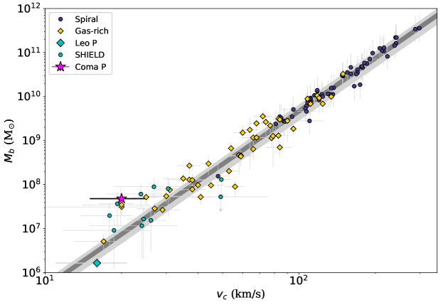
Coma P is shown on the baryonic Tully–Fisher relation (Tully & Fisher, 1977) in Figure 17. The derivations of rotational velocity and baryonic mass use the same techniques for Coma P (§ 5.1) and the low-mass comparison samples (Bernstein-Cooper et al., 2014; McNichols et al., 2016). However, importantly, we stress that the dynamics of Coma P favor a multiple-disk scenario, and therefore it can only be shown on this plot with the estimate of rotation velocity from one of the two kinematic components. We use the inclination-corrected velocity of the more massive component (20 10 km s-1) and the total baryonic mass of the entire Coma P system (which is well represented by the gas mass because the stellar mass is so low). The position of Coma P is highly uncertain and is meant to be demonstrative only.
Compared to the SHIELD galaxies and other systems studied in McNichols et al. (2016), Coma P is slightly offset from the best-fit relation in the plane of Mbary versus Vc, although in agreement within the errors on the measurement of the rotational velocity. However, we stress that the error bars on the estimates of the rotational velocity of Coma P make its placement representative only. Interestingly, while Coma P lies just slightly above the empirical threshold differentiating rotationally-supported and pressure-supported systems that was identified by McNichols et al. (2016), its interpretation is nonetheless very challenging due to its complicated HI gas dynamics.
7 Conclusions
We have presented new HI spectral line imaging of the curious Local Volume dwarf irregular galaxy Coma P (AGC 229385). This source is unique in many respects. It has an extremely low optical surface brightness, complicated HI gas dynamics, and very intriguing patterns of recent star formation. An understanding of the physical properties of this galaxy is important for galaxy evolution in the low-mass regime.
This galaxy is one of three HI line sources detected by ALFALFA at recessional velocities between 1282 and 1343 km s-1 and in close angular proximity to each other. Remarkably, the new HST imaging presented in S. Brunker et al. (2017, in preparation) has shown that Coma P is much closer than the original Virgocentric flow model of Masters (2005) predicted (D 25 Mpc). At D 5.50 0.28 Mpc, the total HI mass is MHI (3.48 0.35) 107 M⊙, reshaping and complicating our interpretive framework for this already enigmatic source. At this time the physical association of Coma P with the other HI line sources (AGC 229384 and AGC 229383) remains unconfirmed, although based on their angular and velocity proximity it is likely that they are all located at roughly the same distance.
Using a combination of deep WSRT and VLA observations, we study the HI properties of Coma P at physical resolutions of 450, 333, and 200 pc. The HI morphology is characterized by two maxima in mass surface density near either end of an inclined HI distribution. The HI disk of Coma P is physically large (diameter 4.00.2 kpc measured at the 1 M⊙ pc-2 level) compared to galaxies of comparable HI mass. Its globally averaged HI surface density is slightly lower than expected based on the known scaling between HI mass and HI diameter. At the same time, it has an exceptionally high ratio of HI mass [MHI (3.480.35) 107 M⊙] to stellar mass [M⋆ (1.00.3) 106 M⊙].
An intrinsically faint dwarf, Coma P’s extreme optical surface brightness renders it completely undetectable in SDSS. Coma P is currently not forming massive stars (as traced by nebular H emission), even though the HI mass surface densities exceed 1021 cm-2 in localized regions. The galaxy has formed stars during the most recent few hundred million years. Far-ultraviolet emission as traced by GALEX images shows good spatial agreement with the high column density HI gas in the inner regions of the galaxy.
The HI kinematics of Coma P are extremely complex and are not well described by a simple tilted ring model. There are highly irregular gas motions and macroscopic velocity gradients at multiple position angles. Using both three-dimensional modeling and spatially resolved position velocity analysis, we find that the HI properties are best described either by two colliding HI disks or by a significant infall event. A coarse separation of these HI components shows that they are of comparable mass.
Using the most obvious signatures of rotation in the three-dimensional data, we estimate the total dynamical mass of the Coma P system to be (1.2 0.6) 108 M⊙. It is important to note that this is the sum of the estimates of the dynamical masses of the two kinematically distinct HI components. Coma P is not unusually dominated by dark matter (Mdyn/Mbary 2.5) compared to other Local Volume dwarf galaxies with similar dynamical masses. In the context of the fundamental MHI–DHI and baryonic Tully–Fisher relations, Coma P is slightly offset from, but in general agreement with, the trends seen for other Local Volume galaxies. We stress that the presence of two HI components complicates the interpretation of these fundamental scaling relations.
The origins of the exceptional physical properties of Coma P may result from one or more infall and/or interaction events. There are HI clouds with similar velocities to that of Coma P in close angular proximity. While we do not detect stellar components of these clouds in deep ground-based images (Janowiecki et al., 2015), if these are in fact physically associated with Coma P then they may suggest a past significant merger event. We refer the reader to the discussions in S. Brunker et al. (2017, in preparation) of the local environment and large-scale structure surrounding Coma P.
Assuming that the irregular kinematics of the HI gas in Coma P do result from a merger of two low-mass disks, then this offers a unique opportunity to compare observations with predictions from simulations. Hydrodynamical simulations with realistic feedback prescriptions are just now able to model halos in the mass range of Coma P (see, for example, the discussion of the “Feedback in Realistic Environments” simulations that are discussed in S. Brunker et al. 2017, in preparation). The unusual gas kinematics in Coma P are qualitatively similar to those shown in the simulations of gas-rich dwarf galaxies and dark companions by Starkenburg et al. (2016). Further, those simulations naturally predict off-center star formation in the resulting merged system - similar to the properties of HI gas and star formation seen in Coma P.
Regardless of their origins, the physical characteristics of Coma P make it an exceptional galaxy. Its physical properties are among the most extreme of any known source in the Local Volume. Coma P will serve as a critical benchmark for our understanding of low-mass galaxy evolution.
References
- Adams et al. (2013) Adams, E. A. K., Giovanelli, R., & Haynes, M. P. 2013, ApJ, 768, 77
- Adams et al. (2015) Adams, E. A. K., Faerman, Y., Janesh, W. F., et al. 2015, A&A, 573, L3
- Adams et al. (2016) Adams, E. A. K., Oosterloo, T. A., Cannon, J. M., Giovanelli, R., & Haynes, M. P. 2016, A&A, 596, A117
- Bernstein-Cooper et al. (2014) Bernstein-Cooper, E. Z., Cannon, J. M., Elson, E. C., et al. 2014, AJ, 148, 35
- Broeils & Rhee (1997) Broeils, A. H., & Rhee, M.-H. 1997, A&A, 324, 877
- Cannon et al. (2011a) Cannon, J. M., Giovanelli, R., Haynes, M. P., et al. 2011, ApJ, 739, L22
- Cannon et al. (2011b) Cannon, J. M., Most, H. P., Skillman, E. D., et al. 2011, ApJ, 735, 35
- Cannon et al. (2015) Cannon, J. M., Martinkus, C. P., Leisman, L., et al. 2015, AJ, 149, 72
- Cannon et al. (2016) Cannon, J. M., McNichols, A. T., Teich, Y. G., et al. 2016, AJ, 152, 202
- Carignan & Purton (1998) Carignan, C., & Purton, C. 1998, ApJ, 506, 125
- Giovanelli et al. (2005) Giovanelli, R., Haynes, M. P., Kent, B. R., et al. 2005, AJ, 130, 2598
- Giovanelli et al. (2013) Giovanelli, R., Haynes, M. P., Adams, E. A. K., et al. 2013, AJ, 146, 15
- Haynes et al. (2011) Haynes, M. P., Giovanelli, R., Martin, A. M., et al. 2011, AJ, 142, 170
- Hirschauer et al. (2016) Hirschauer, A. S., Salzer, J. J., Skillman, E. D., et al. 2016, ApJ, 822, 108
- Huang et al. (2012) Huang, S., Haynes, M. P., Giovanelli, R., et al. 2012, AJ, 143, 133
- Janesh et al. (2015) Janesh, W., Rhode, K. L., Salzer, J. J., et al. 2015, ApJ, 811, 35
- Janesh et al. (2017) Janesh, W., Rhode, K. L., Salzer, J. J., et al. 2017, ApJ, 837, L16
- Janowiecki et al. (2015) Janowiecki, S., Leisman, L., Józsa, G., et al. 2015, ApJ, 801, 96
- Jörsäter & van Moorsel (1995) Jörsäter, S., & van Moorsel, G. A. 1995, AJ, 110, 2037
- Józsa et al. (2007) Józsa, G. I. G., Kenn, F., Klein, U., & Oosterloo, T. A. 2007, A&A, 468, 731
- Leisman et al. (2016) Leisman, L., Haynes, M. P., Giovanelli, R., et al. 2016, MNRAS, 463, 1692
- Leisman et al. (2017) Leisman, L., Haynes, M. P., Janowiecki, S., et al. 2017, ApJ, 842, 133
- Leisman (2017) Leisman, L. 2017, Ph.D. Thesis, Cornell University
- Masters (2005) Masters, K. L. 2005, Ph.D. Thesis, Cornell University
- Matsuoka et al. (2012) Matsuoka, Y., Ienaka, N., Oyabu, S., Wada, K., & Takino, S. 2012, AJ, 144, 159
- McGaugh et al. (2018) McGaugh, S., Schombert, J., & Lelli, F. 2018, ApJ, in press (ArXiV/1710.11236)
- McMullin et al. (2007) McMullin, J. P., Waters, B., Schiebel, D., Young, W., & Golap, K. 2007, ADASS XVI, 376, 127
- McNichols et al. (2016) McNichols, A. T., Teich, Y. G., Nims, E., et al. 2016, ApJ, 832, 89
- McQuinn et al. (2013) McQuinn, K. B. W., Skillman, E. D., Berg, D., et al. 2013, AJ, 146, 145
- McQuinn et al. (2015a) McQuinn, K. B. W., Cannon, J. M., Dolphin, A. E., et al. 2015, ApJ, 802, 66
- McQuinn et al. (2015b) McQuinn, K. B. W., Skillman, E. D., Dolphin, A. E., & Mitchell, N. P. 2015, ApJ, 808, 109
- McQuinn et al. (2015c) McQuinn, K. B. W., Skillman, E. D., Dolphin, A., et al. 2015, ApJ, 812, 158
- McQuinn et al. (2015d) McQuinn, K. B. W., Skillman, E. D., Dolphin, A., et al. 2015, ApJ, 815, L17
- Oh et al. (2015) Oh, S.-H., Hunter, D. A., Brinks, E., et al. 2015, AJ, 149, 180
- Rhode et al. (2013) Rhode, K. L., Salzer, J. J., Haurberg, N. C., et al. 2013, AJ, 145, 149
- Singer et al. (2017) Singer, Q., Ball, C., Cannon, J. M., et al. 2017, American Astronomical Society Meeting Abstracts, 229, 145.10
- Skillman (1987) Skillman, E. D. 1987, NASA Conference Publication, 2466, 263
- Skillman et al. (2013) Skillman, E. D., Salzer, J. J., Berg, D. A., et al. 2013, AJ, 146, 3
- Sorgho et al. (2017) Sorgho, A., Hess, K., Carignan, C., & Oosterloo, T. A. 2017, MNRAS, 464, 530
- Starkenburg et al. (2016) Starkenburg, T. K., Helmi, A., & Sales, L. V. 2016, A&A, 595, A56
- Teich et al. (2016) Teich, Y. G., McNichols, A. T., Nims, E., et al. 2016, ApJ, 832, 85
- Tully & Fisher (1977) Tully, R. B., & Fisher, J. R. 1977, A&A, 54, 661
- van der Hulst et al. (1992) van der Hulst, J. M., Terlouw, J. P., Begeman, K. G., Zwitser, W., & Roelfsema, P. R. 1992, ADASS I, 25, 131
- Wang et al. (2016) Wang, J., Koribalski, B. S., Serra, P., et al. 2016, MNRAS, 460, 2143
- Warren et al. (2015) Warren, S. R., Molter, E., Cannon, J. M., et al. 2015, ApJ, 814, 30