On the existence of a luminosity threshold of GRB jets in massive stars

Abstract

Motivated by the many associations of $\gamma$-ray bursts (GRBs) with energetic supernova (SN) explosions, we study the propagation of relativistic jets within the progenitor star in which a SN shock wave may be launched briefly before the jets start to propagate. Based on analytic considerations and verified with an extensive set of 2D axisymmetric relativistic hydrodynamic simulations, we have estimated a threshold intrinsic jet luminosity, $L_{\rm j}^{\rm thr}$, for successfully launching a jet. This threshold depends on the structure of the progenitor and, thus, it is sensible to its mass and to its metallicity. For a prototype host of cosmological long GRBs, a low-metallicity star of 35 $M_{\odot}$, it is $L_{\rm j}^{\rm thr}\simeq 1.35\times 10^{49}$ erg s^-1. The observed equivalent isotropic $\gamma$-ray luminosity, $L_{\rm\gamma,iso,BO}\simeq 4\epsilon_{\gamma}L_{\rm j}\theta_{\rm BO}^{-2}$, crucially depends on the jet opening angle after breakout, $\theta_{\rm BO}$, and on the efficiency for converting the intrinsic jet luminosity into $\gamma$-radiation, $\epsilon_{\gamma}$. Highly energetic jets can produce low-luminosity events if either their opening angle after the breakout is large, which is found in our models, or if the conversion efficiency of kinetic and internal energy into radiation is low enough. Beyond this theoretical analysis, we show how the presence of a SN shock wave may reduce this luminosity threshold by means of numerical simulations. We foresee that the high-energy transients released by jets produced near the luminosity threshold will be more similar to llGRBs or XRFs than to GRBs.

1 Introduction

The association of long gamma-ray bursts (GRBs) with supernovae (SNe; in particular with broad-lined Type Ic SNe, SNe Ic-bl) has been observationally confirmed at low redshifts (typically, $z\lesssim 0.3$ Galama et al. 1998; Patat et al. 2001; Hjorth et al. 2003; Stanek et al. 2003; Malesani et al. 2004; Pian et al. 2006; Bufano et al. 2012; Hjorth 2013; Modjaz et al. 2016; Cano et al. 2017). The detection of these two events together plays in favor of the collapsar model (Woosley, 1993; MacFadyen & Woosley, 1999) and points towards Wolf-Rayet (WR) stars with masses $>10M_{\odot}$ as the likeliest candidates to host the central engines of long GRBs (Woosley, 1993; Kumar & Zhang, 2015). The inferred explosion energy of these SNe is at least ten times larger ($E_{\rm HN}>10^{52}$ erg) than that of typical SNe (see, e.g. Woosley & Bloom 2006), which is why they are referred in the literature as hypernovae (HNe, Paczyński 1998; Iwamoto et al. 1998). However the associated GRBs display a large variety of isotropic energies. A good number of the confirmed events have GRBs classified as low luminosity bursts (llGRBs), because they show equivalent isotropic luminosities in the range $L_{\rm\gamma,iso}\sim 10^{46}$–$10^{48}\,$erg s^-1 (to be compared with typical values of $L_{\rm\gamma,iso}\sim 10^{50}$–$10^{53}\,$erg s^-1 for LGRBs; see, e.g. Hjorth 2013). In addition to being less luminous than canonical long GRBs, and despite some of them showing very long durations ($\lesssim 1000$ s), llGRBs also seem to be less energetic than the latter (holding equivalent isotropic energies $E_{\rm\gamma,iso}\sim 10^{48}$–$\text{few}\,\times 10^{49}\,$erg; i.e. two to three orders of magnitude smaller than canonical GRBs), are softer ($E_{\rm p}<100$ keV), display relatively smooth (non-variable) light curve (LC), and show no evidence for a high-energy power-law tail (e.g. Bromberg et al., 2011a).

The atypical prompt emission, the origin of X-ray blackbody (BB) components, and the unusual X-ray afterglow shown in many GRB/SN associations, especially in the case of llGRBs (e.g. llGRBs 060218; Campana et al. 2006, 100316D; Starling et al. 2011; Cano et al. 2011, although not restricted to them; see e.g. Page et al. 2011 for GRB 090618) are difficult to fit in terms of standard GRB theory. In light of the current observational data, it is still unclear whether progenitors of llGRBs are the same as that of cosmological GRBs or whether these super-long llGRBs are members of a low-luminosity end of a continuum of collapsar explosions or, maybe, a different stellar endpoint. Answering these questions has important implications for high-mass stellar evolution, the connection between SNe and GRBs, and the low-energy limits of GRB physics, especially taking into account that llGRBs are likely more frequent than cosmological GRBs (Coward, 2005; Cobb et al., 2006; Pian et al., 2006; Soderberg et al., 2006; Liang et al., 2007; Guetta & Della Valle, 2007; Fan et al., 2011). In particular, Soderberg et al. (2006) calculated that the rate of SNe Ic-bl is about the same as that of llGRBs, implying that llGRBs cannot be significantly beamed. Indeed, it is likely that llGRBs are even isotropic and the result of “failed” jets (e.g. Bromberg et al., 2011a), i.e. jets which become partly choked in the stellar envelope. Due to the lack of prompt observations in GRB/SN detection it is poorly understood how an outgoing shock (relativistic or not) punches out its progenitor star. In the collapsar model a relativistic jet must successfully break out of its progenitor in order to produce a canonical LGRB. Before the typical non-thermal radiation associated to the flash in $\gamma$/X-rays caused by the breakout, the SN shock breakout may produce some sort of thermal signal (Campana et al.,, 2006; Waxman, Mészáros & Campana, 2007; Soderberg et al.,, 2008; Nakar & Sari, 2012; Nakar, 2015; Irwin & Chevalier, 2016). Observations in the last ten years are pointing towards this direction. In particular the llGRB 060218, associated to SN 2006aj, shows a thermal component in X-rays which cools as it moves to optical frequencies (Campana et al., 2006). Based on the analysis of such observations, the authors argue that the BB emission may arise from a SN shock wave breaking out the extended wind surrounding a WR star. More recently, Nakar (2015) has suggested that both canonical LGRBs and llGRBs may have a similar origin. The similar properties inferred from the associated SNe in both kinds of bursts suggest the existence of similar progenitors with modified environments. The optical LCs of the llGRB 060218, with a two peak structure, suggest the presence of an extended low-mass envelope at a distance of $10^{13}$–$10^{14}$ cm that could also explain the observable differences at high energies (see also Irwin & Chevalier 2016). This envelope would brake the incipient relativistic jet and would dissipate part of the energy choking the jet that would emerge at much lower speeds without producing a typical burst signal. Similar qualitative conclusions have been obtained for the GRB 100316D/SN 2010bh (Starling et al., 2011) and for the GRB 140606B /SN iPTF14bfu (Singer et al., 2015; Cano et al., 2015). The wide GRB energy ranges observed could be explained on the basis of progenitor-dependent wind properties that might give rise to jets with different conditions, with the relativistic ones as those that would produce the most energetic bursts. Low luminosity GRBs may be generated by mildly relativistic or even almost ‘failed’ jets (see above).

Our main goal here is to show that standard, low-metallicity stellar progenitors of LGRBs may not produce relativistic jets of sufficiently low luminosity to account for the least luminous end of the distribution of llGRBs, unless either the produced jets undergo a substantial broadening of their opening angle after they break out of the surface of the stellar progenitor, or the radiative efficiency in the gamma ray band is really small. Indeed, we will show analytically (Sec. 2) the existence of a luminosity threshold below which, jet injection conditions are not well posed, since jets must be supersonic with respect to the reference frame attached to the progenitor star. This finding should be added to the previous criteria for the production of LGRBs found by Bromberg et al. (2011a), inasmuch as the threshold we obtain is not set by the time over which the central engine is efficiently pumping energy into a relativistic outflow compared to the jet crossing time of the stellar progenitor. In order to check the validity of our analytic conclusions, we have developed a detailled numerical model (Sec. 3) that encompasses all the elements which are relevant to set the former threshold, i.e. the structure of the massive stellar progenitor and its circumstellar medium (a WR surrounded by an inflated envelope), and the possible existence of a SN shock launched in addition to the injection of a relativistic jet. Following the ideas of Nakar (2015), in this paper we work under the hypothesis that the stellar progenitor is the same for canonical LGRBs, llGRBs and SN Ic explosions. For such reason we assume that a relativistic jet and a SN ejecta can form inside of the stellar progenitor. Which outflow forms first is still unclear, although numerical simulations suggest that the SN would form first (Obergaulinger & Aloy, 2017). In this work, we consider all possibilities. In Section 4, we contrast the analytical results with simulations and we study the propagation of relativistic jets within a WR star which may (or may not) have formed a previous SN shock wave. In Section 5, we discuss our results in view of the existence of a luminosity threshold constraining the generation of low-luminosity transients in potential stellar progenitors of LGRBs/llGRBs.

2 Luminosity threshold for jet injection and llGRBs production

A GRB jet can be launched inside of a massive star if a suitable physical mechanism, which so far is not totally understood, extracts sufficient energy from the central engine. The jet will propagate subrelativistically within the star and eventually will break out of the star relativistically after a time $t_{\rm b}$ (e.g. Aloy et al. 2000), before giving rise to the $\gamma$-ray emission. To do so the central engine must be active a time $t_{\rm e}>t_{\rm b}$ to compensate for the energy dissipated in the jet in its way through the star. Many numerical studies have been carried out investigating the propagation of relativistic jets in collapsars, either in 2D (e.g. MacFadyen & Woosley, 1999; Aloy et al., 2000; MacFadyen et al., 2001; Zhang et al., 2003, 2004; Mizuta et al., 2006; Morsony et al., 2007, 2010; Lazzati & Begelman, 2010; Mizuta & Aloy, 2009; Lazzati et al., 2009; Nagakura et al., 2011; Lazzati et al., 2013; López-Cámara et al., 2014) and also in 3D (e.g. Zhang et al., 2003; López-Cámara et al., 2013; Ito et al., 2015; López-Cámara et al., 2016; Bromberg & Tchekhovskoy, 2016).

Should the progenitors of both LGRBs and llGRBs be the same (Nakar, 2015), it would be natural to assume that llGRBs correspond to the low luminosity tail of LGRBs. However, relativistic jets injected with a luminosity below a threshold that we may estimate analytically, fail to penetrate the stellar envelope and, hence, they won’t produce a llGRB. We shall show in this section that the latter luminosity threshold is too large to explain events with luminosities $\lesssim 10^{48}\,$erg s^-1 in standard LGRB progenitors.

Let us assume that a relativistic jet has already been formed and that it has developed some fiducial conditions at radial distances sufficiently much larger than the pre-collapsed iron core ($\gtrsim 10^{9}$ cm), e.g. a well defined cross-sectional injection radius, $R_{\rm j}$, a relatively small half-opening angle $\theta_{\rm j}\ll 1$ and a bulk Lorentz factor $\Gamma_{\rm j}=(1-v_{\rm j}^{2})^{-1/2}>1$ (where $v_{\rm j}$ is the velocity of the beam). Under these conditions, the complex problem of jet formation in the vicinity of the central engine can be replaced by the injection of a relativistic flow through a relatively narrow nozzle. The jet injection conditions must guarantee that the outflow is supersonic with respect to the external medium (otherwise, the mathematical injection problem is not well-posed). That means that at the injection point the velocity of the jet’s head, $v_{\rm h}$, must be larger than the speed of sound of the medium, $c_{\rm s,a}$, i.e.

$$v_{\rm h}>c_{\rm s,a}.$$ (1)

If, for simplicity, we neglect the gravitational pull of the star and assume that the stellar matter is at rest, the velocity of the jet’s head can be approximated by (Martí et al., 1997; Matzner, 2003; Bromberg et al., 2011b)

$$v_{\rm h}=\frac{v_{\rm j}}{1+\tilde{L}^{-1/2}}\,,$$ (2)

where

$$\tilde{L}\equiv\frac{\rho_{\rm j}h_{\rm j}\Gamma_{\rm j}^{2}}{\rho_{\rm a}}\simeq\frac{L_{\rm j}}{S_{\rm j}\rho_{\rm a}c^{3}}\,,$$ (3)

where $L_{\rm j}$ is the jet luminosity, $h_{\rm j}$ is the specific enthalpy of the jet and

$$S_{\rm j}=\pi R_{\rm j}^{2}\sin{\theta_{\rm j}}^{2}\approx\pi R_{\rm j}^{2}\theta_{\rm j}^{2}$$ (4)

is the jet’s cross section. The indices ‘j’ and ‘a’ refer to properties of the jet and the ambient medium, respectively. Since the stellar density is much larger than the jet density, i.e. $\rho_{\rm j}/\rho_{\rm a}\ll 1$ and for typical GRB jet conditions the asymptotic Lorentz factor $\Gamma_{\infty}:=h_{\rm j}\Gamma_{\rm j}>100$ and $1<h_{\rm j}\gtrsim 20$ (the upper bound would correspond to a rather hot outflow and is only given for reference) we expect, $\tilde{L}\ll 1$. Then, using Eq. (1) we obtain

$$\frac{v_{\rm h}}{c_{\rm s,a}}\simeq\frac{\tilde{L}^{1/2}}{c_{\rm s,a}}>1$$ (5)

From this condition, and using Eq. (12) and (4), we estimate the minimum luminosity that a jet with a half-opening angle $\theta_{\rm j}$ must have at the injection point, $R_{\rm j}=R_{\rm inj,j}$, namely, $L_{\rm j}\gtrsim L_{\rm j}^{\rm thr}$, where

$$\begin{split}L_{\rm j}^{\rm thr}:=&\,1.4\times 10^{49}\\ &\times\left(\frac{R_{\rm j}}{2\times 10^{9}\,\text{cm}}\right)^{2}\left(\frac{\theta_{\rm j}}{2^{\circ}}\right)^{2}\left(\frac{p_{\rm a}}{1.8\times 10^{22}\,\text{erg\,cm${}^{-3}$}}\right)\,\text{erg s${}^{-1}$}\,,\end{split}$$ (6)

where we have scaled the ambient medium pressure at $R_{\rm inj,j}$ employing typical values of the stellar progenitor 35OC (see Sec. 3.1) at $R_{\rm inj,j}$. Also, we have taken an injection half-opening angle ($\theta_{\rm j}=2^{\circ}$) as small as possible to minimize the obtained luminosity threshold but, at the same time, compatible with a hydrodynamic or MHD jet generation. To convert the previous jet intrinsic luminosity into an equivalent isotropic quantity we employ $L_{\rm iso,j}=2L_{\rm j}/(1-\cos{\theta})\simeq 4L_{\rm j}/\theta^{2}$ where $\theta=\theta_{j}$ at the injection point. Likewise, if this luminosity is maintained for an injection time $t_{\rm inj,j}$, after which it is shut down progressively (see Sec. 3.4), we obtain an equivalent isotropic energy from $E_{\rm iso,j}=L_{\rm iso,j}\times(4/3)\,t_{\rm inj,j}$; where the factor $4/3$ takes into account the shut down phase of the injection. Thus, at the injection point:

$$L_{\rm iso,j}\gtrsim 4.5\times 10^{52}\,\left(\frac{R_{\rm j}}{2\times 10^{9}\,\text{cm}}\right)^{2}\left(\frac{p_{\rm a}}{1.8\times 10^{22}\,\text{erg\,cm${}^{-3}$}}\right)\,\text{erg s${}^{-1}$}\,,$$ (7)

and

$$\begin{split}E_{\rm iso,j}\gtrsim 1.2\times 10^{54}\,&\left(\frac{R_{\rm j}}{2\times 10^{9}\,\text{cm}}\right)^{2}\\ \times&\left(\frac{p_{\rm a}}{1.8\times 10^{22}\,\text{erg\,cm${}^{-3}$}}\right)\left(\frac{t_{\rm inj,j}}{20\,\text{s}}\right)\,\text{erg}\,.\end{split}$$ (8)

We note that the former estimates of the isotropic jet luminosity and energy have been made assuming that the value of the outflow half-opening angle is the same asymptotically as it is initially. Nevertheless, according to Mizuta & Ioka (2013), after the jet breakout the opening angle of the jet becomes $\theta_{\rm BO}\simeq 1/(5\Gamma_{\rm j})$. The value of the beam bulk Lorentz factor at the injection point shall be rather moderate, since it is very close to the stagnation point from where the outflow is launched. Thus, the acceleration of the beam has not finished yet, and most of it may happen while the jet is travelling through the outer stellar layers and after the jet break out (e.g. Aloy et al., 2000; Mizuta & Ioka, 2013). In practical terms, $\Gamma_{j}\lesssim 10$ are likely values for the jet injection Lorentz factor. For the purposes of this estimate, we use $\Gamma_{\rm j}=5$ (see Sec. 3.4) and, therefore, we would obtain $\theta_{\rm B0}\simeq 2.3^{\circ}\simeq\theta_{j}$, so that the previous thresholds for both the isotropic luminosity (Eq. 7) and for the isotropic energy (Eq. 8) of the jet would remain at breakout since=

$$L_{\rm iso,BO}\simeq 4L_{\rm j}/\theta_{\rm BO}^{2}\simeq L_{\rm iso,j}\,,$$ (9)

and also $E_{\rm iso,BO}\simeq E_{\rm iso,j}$.

Hence, if the results of Mizuta & Ioka (2013) hold, we do not expect any jets that manage to propagate supersonically in the pre-supernova model 35OC to fall into the category of llGRBs, unless the radiative efficiency in the $\gamma-$ray band, $\epsilon_{\gamma}=L_{\rm iso,\gamma}/L_{\rm iso}$, is very small ($\epsilon_{\gamma}\lesssim 10^{-4}$). However, the breakout angle can be significantly larger than predicted by Mizuta & Ioka (2013) for jets injected in the stellar progenitor model 16TI of Woosley & Heger (2006), especially if the jet luminosity is very close to the threshold we have found (see Sec. 4). Indeed, we expect $\theta_{\rm BO}\sim a/\Gamma_{\rm j}$, with $0.5<a\lesssim 3$. This larger breakout angle translates into the following constrains on the isotropic luminosity and energy:

$$\begin{split}L_{\rm\gamma,iso,BO}\gtrsim\,1.5\times 10^{48}\,&\left(\frac{\epsilon_{\gamma}}{0.01}\right)\,\left(\frac{R_{\rm j}}{2\times 10^{9}\,\text{cm}}\right)^{2}\left(\frac{\theta_{\rm j}}{2^{\circ}}\frac{35^{\circ}}{\theta_{\rm BO}}\right)^{2}\\ \times&\left(\frac{p_{\rm a}}{1.8\times 10^{22}\,\text{erg\,cm${}^{-3}$}}\right)\,\text{erg s${}^{-1}$}\,,\end{split}$$ (10)

and

$$\begin{split}E_{\rm\gamma,iso,BO}\gtrsim\,3.9\times 10^{49}\,&\left(\frac{\epsilon_{\gamma}}{0.01}\right)\left(\frac{R_{\rm j}}{2\times 10^{9}\,\text{cm}}\right)^{2}\left(\frac{\theta_{\rm j}}{2^{\circ}}\frac{35^{\circ}}{\theta_{\rm BO}}\right)^{2}\\ \times&\left(\frac{p_{\rm a}}{1.8\times 10^{22}\,\text{erg\,cm${}^{-3}$}}\right)\left(\frac{t_{\rm inj,j}}{20\,\text{s}}\right)\,\text{erg}.\end{split}$$ (11)

Therefore, it is possible to host in model 35OC jets, which would have isotropic equivalent luminosities consistent with the upper bound of llGRBs if, as suggested by our models (see next Sec. 4), the breakout opening angle grows well above the expectations of Mizuta & Ioka (2013), and if the acceptable radiative efficiency is $\epsilon_{\gamma}\lesssim 1\%$.

The jet equivalent isotropic energy threshold (Eq. 8) depends upon three factors. One of them, $t_{\rm inj}$, is an intrinsic jet property, which cannot be much shorter than $\sim 20\,$s, if we aim to produce jets which release $\gamma-$radiation over time scales compatible with llGRBs or LGRBs. The ambient medium pressure at $R_{\rm j}$ may be different depending on the radial distance at which we inject the jet. In order to assess the robustness of the criterion found, we have computed the equivalent isotropic energy as a function of the radius (Eq. 8) for a jet to form with an intrinsic luminosity right at the threshold found in Eq. (6). For this purpose, we assume that the outflow half-opening angle is kept approximately constant and equal to $\theta_{\rm j}$. The results for two different progenitors and different variations of the physical conditions inside them are shown in Fig. 1. The blue line corresponding to progenitor model 35OC shows that jets with $E_{\rm iso,j}^{\rm thr}\lesssim 10^{54}$ erg cannot be launched unless the injection radius is $R_{\rm j}\gtrsim 6\times 10^{9}$ cm. Beyond this distance, and up to $R_{\rm j}\simeq 2\times 10^{10}\,$cm only jets with $E_{\rm iso,j}^{\rm thr}\gtrsim 10^{52}$ erg can be launched. The reduction in the luminosity threshold for $R_{\rm j}\gtrsim 6\times 10^{9}$ cm is produced by the quick decline of the pressure (and hence of the $c_{\rm s,a}$) in the envelope of the stellar progenitor. But even if jet fiducial conditions would set in the stellar envelope, $L_{\rm iso,j}$ would be only marginally compatible with the luminosities observed for the most powerful llGRBs.

In order to reduce the luminosity threshold found in Eq. (6), we may seek ways to reduce the pressure or the density of the stellar progenitor model. One possibility to obtain the sought effect is including a SN shock wave that propagates from the outer stellar core towards the stellar surface. We mimic the global effect of such a SN shock wave (see Sec. 3.3) setting it up with a “piston” mechanism assuming spherical symmetry and injecting the SN in our stellar progenitor model at a radial distance $R_{0}=10^{9}\,$cm (App. A). The SN shock wave possesses an energy, $E_{\rm SN}=10^{52}\,$erg, and we let it propagate inside of the 35OC stellar model up to a distance of $\sim 5\times 10^{9}\,$cm by the time we compute the local values of $L_{\rm j}^{\rm thr}$ and of $E_{\rm iso,j}^{\rm thr}$ that are displayed in Fig. 1 (magenta line). As a result of the passage of the SN shock the density in its wake decreases substantially and lowers significantly the luminosity threshold (by about one order of magnitude) to launch a jet up to $\sim 3\times 10^{9}\,$cm. Beyond that radial distance, the lines corresponding to the thresholds in the original 35OC model (blue line in Fig. 1) and the SN exploding model (magenta line) cross. Remarkably, if we inject a jet with a delay of a few seconds after the passage of the SN shock at a distance of $\sim 10^{9}\,$cm, the jet’s head will be initially supersonic even if it is launched with a luminosity of about one order of magnitude smaller than in the original progenitor (where the reduced luminosity would not allow for a successful jet initiation). We note that, fixed the injection radius, e.g. at $R_{\rm j}\sim 10^{9}\,$cm, the reduction in the luminosity injection threshold is proportional to the time delay between the passage of the SN shock by $r=R_{\rm j}$ and the injection of the jet; the longer the delay, the lower the luminosity threshold to initiate the jet. Nevertheless, we do not expect that the time delays between the SN shock and the jet injection be much longer than a few seconds (see Sec. 3.4) and, thereby, the reduction of the luminosity threshold should not be much larger than depicted in Fig. 1. This means that, even if the SN shock precedes the jet injection, the expected equivalent isotropic luminosity of a potentially succesful jet would not be low enough to account for most of the lower luminosity llGRBs. We further note that the SN shock compresses the stellar matter and, as a result, the luminosity threshold is larger than that corresponding to the unperturbed stellar progenitor in a fraction of the shocked region, namely, in the region $3\lesssim R_{9}\lesssim 5$; Fig. 1. Should the jet be initiated below this region, it would interact with the SN shocked matter and, depending on its intrinsic luminosity, it could be choked inside the start (see Sec.3.4).

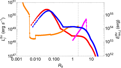
Figure 1: Intrinsic luminosity threshold (Eq. 6; left scale) and equivalent isotropic energy threshold (Eq. 8; right scale) for different progenitor models: pre-supernova models 35OC (blue) and 16TI (red) of Woosley & Heger 2006, and initial model of the series J3 (Tab. 1) of this work (magenta). The latter models include a SN shock wave set up with an energy $E_{\rm SN}=10^{52}$ erg. We also include data computed for the density profile of one of the pre-supernova models of Obergaulinger & Aloy 2017, corresponding at the moment of BH formation after the core collapse of model 35OC (orange). The vertical dashed line shows the position of $R_{\rm inj}(\emph{Jet})$. The radius is expressed in units of $10^{9}$ cm, $R=R_{9}10^{9}$ cm. Each of the models displayed in the figure is computed on a different radial grid. The stellar models 16TI and 35OC on the original radial grid of Woosley & Heger 2006, while models J3 are computed on a grid where the central part of the 35OC progenitor ($R_{9}<1$) is excised and that extends to the stelar radius $R_{\ast}$ (Sec. 3). Finally, the model evolved to the brink of BH collapse is computed on a grid spaning $R_{9}<2.5$. In all cases, we assume that jets are injected with a half-opening angle $\theta_{\rm j}=2^{\circ}$. Note that we have assumed that the breakout half-opening angle equals $\theta_{\rm j}$ in order to compute $E_{\rm iso,j}^{\rm thr}$.

Admittedly, the set up of the SN shock wave by means of a piston mechanism may be an oversimplification of the (much) more involved process of SN shock generation mechanism. Thus, we have also evaluated the jet luminosity threshold and the corresponding value of $E_{\rm iso,j}^{\rm thr}$ as a function of radius for a more realistic model. Figure 1 (orange line) also includes the profile of a pre-supernova model of Obergaulinger & Aloy (2017; orange line; model OA17 hereafter), evolved from the onset of core collapse in the progenitor 35OC until BH formation. We chose a non-exploding model for this comparison in order to study how much the decrease of the gas density in the core due to the accretion of matter onto the proto-neutron star lowers the threshold for jet production. By the end of the simulation, the layers at the distance of our injection location are still unaffected by the dynamics of the core collapse and, thus, there is effectively no difference in the luminosity threshold for jet initiation with respect to our reference 35OC model for $R_{9}\geq 1$. The tiny differences observed close to $R_{\rm inj}(\emph{Jet})$ (identified by the vertical dashed line in the figure) are due to the influence of the boundary conditions in the simulations of Obergaulinger & Aloy, whose numerical grid spans the region contained up to $R_{9}=2.5$ (since they are mostly interested in the dynamics of the central engine). We remark that in the more realistic initial profile of model OA17, their fiducial jet injection conditions are set deeper inside than in our model (e.g. at $0.1R_{9}$), the luminosity threshold decreases by a factor $\sim 5$ with respect to our reference 35OC model initiating the jet at $R_{\rm inj}(\emph{Jet})$. Nonetheless, this reduction is still insufficient to drive a supersonic jet inside the grid with a luminosity compatible with that of llGRBs.

In order to explore the progenitor dependence of the luminosity threshold, we depict the values of $L_{\rm j}^{\rm thr}$ and of $E_{\rm iso,j}^{\rm thr}$ for another GRB progenitor candidate, the pre-supernova model 16TI of Woosley & Heger (2006). For this model both the luminosity and the energy threshold is smaller than that of the model 35OC above $10^{8}$ cm, e.g. by a factor 5 around $10^{9}$ cm. However, as in all the previous cases, the reduction in the luminosity threshold does not suffice for the purpose of initiating a llGRB jet, if the jet breakout opening angle is similar to the jet injection half-opening angle and the radiative efficiency is not as low as $\epsilon_{\gamma}\simeq 10^{-3}$ (see the discussion below Eq. (11)).

3 The numerical model

In order to test the analytic results for the existence of a luminosity threshold obtained in Sec. 2, we have set up a number of numerical models. These models include the massive stelar progenitor 35OC (Sec. 3.1) endowed with an extended envelope characteristic of WR stars (Sec. 3.2). Furthermore, we may include the effects of a parametrized SN shock wave (Sec. 3.3) modifying the profile of the stellar progenitor in which relativistic jets of different luminosities (close to the thresholds found in Sec. 2) are injected (Sec. 3.4). The simulations have been performed with the relativistic hydrodynamics code MRGENESIS (Aloy et al., 1999; Leismann et al., 2005; Mimica et al., 2009). We modelled the outflows, the stellar gas and the circumstellar medium using the TM equation of state (Mignone et al., 2005; Mignone & McKinney, 2007), which, while not accounting for the detailed chemical composition of the gas and for radiation, is a valid approximation in our case. For resolving the large gradients between the outflows and the stellar profile, we have used the third-order spatial reconstruction scheme PPM (Colella & Woodward, 1984). In order to maintain the hydrostatic equilibrium of the star, we considered its self-gravity by including a Newtonian gravitational potential in MRGENESIS (App. B).

The numerical evolution of our models has been divided in two steps. Firstly, we perform 1D simulations of SN ejecta propagating into the progenitor star (Sec. 3.3). Secondly, we perform 2D simulations of relativistic jets propagating into (1) the medium left behind by the SN ejecta or (2) the progenitor star without modification (Sec. 3.4).

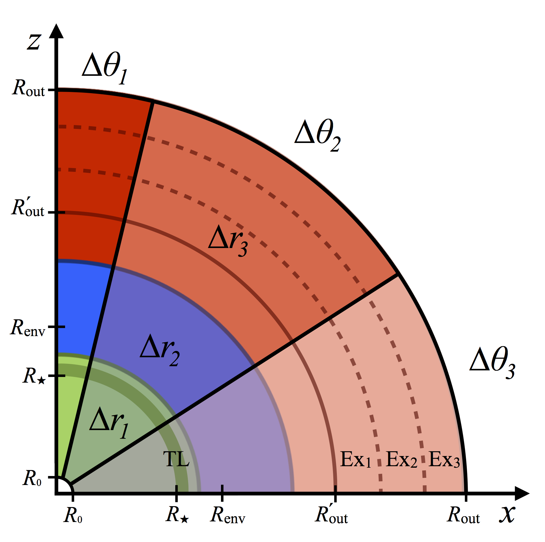
Figure 2: Sketch of the numerical grid. We use three subgrids with different levels of refinement along both radial (green, blue and red) and angular directions (dark to lighter colours). The stellar surface ($R_{\star}$), the transition layer (TL; dark green annulus; included in the first level of refinement of the radial grid), the envelope extension ($R_{\rm env}$) and the the initial ($R^{\prime}_{\rm out}$) and final length of the radial grid ($R_{\rm out}$) after the inclusion of three extra chunks (denoted as ’Ex’) are marked in the figure. Note that the sketch particularly describes the grid setup in model SN. For jet simulations the sketch is equally valid but $R_{0}$ should be replaced by $R_{\rm inj,j}$. Furthermore, we stress that $R^{\prime}_{\rm out}$ and $R_{\rm out}$ have different values and that only two extra chunks, with a different extension than those in model SH, are added to the grid in jet models. See the text for more details. Figure is not to scale.

The numerical resolution of the two-dimensional spherical grid is the result of a trade-off between the computational cost and several factors demanding spatially extended and fine grids. On the one hand, we need to resolve the small scales within the star to properly resolve the jet/star interaction. On the other hand, we need to go to larger length scales as we have to let the jet evolve up to very late times. Obviously, in 1D we could employ much finer numerical grids. Nevertheless, much larger resolutions are not viable in the subsequent computational phase in 2D (Sec. 3.4). Our choice has been to use a nested grid composed of three different uniform-space subgrids (Fig. 2), covering the range $[R_{\rm inj},R^{\prime}_{\rm out}]=[10^{9},2\times 10^{12}]\,$cm. The first radial subgrid has $n_{\rm r,1}=1200$ zones and covers the range $[R_{\rm inj},6.1\times 10^{10}\,$cm] (i.e. the resolution is $\Delta r_{1}=5\times 10^{7}$ cm), while the second one has $n_{\rm r,2}=9400$ zones and covers the range $(6.1\times 10^{10}\,,10^{12}$] cm ($\Delta r_{2}=10^{8}$ cm) and the third one has $n_{\rm r,3}=2500$ zones and covers the range $(1,2]\times 10^{12}$ cm ($\Delta r_{3}=2\times 10^{8}$ cm). Since our models need to be run for a rather long time, the set up flows may eventually reach the limit of the basic grid sketched above. When this happens, we extend the computational domain in the radial direction. The extension is done by adding chunks of external medium with the same resolution as in the third level ($\Delta r_{3}$). The injection radius, $R_{\rm inj}$, for the different outflows we consider (the SN ejecta and the jet) is different in each of the cases ($R_{\rm inj}(\emph{SN})=R_{0}=10^{9}$ cm and $R_{\rm inj}(\text{\emph{Jet}})=2R_{0}=2\times 10^{9}$ cm).

3.1 The progenitor star

As progenitor star, we have chosen the most massive star evolved by Woosley & Heger (2006) that has enough rotational energy to be considered a GRB candidate: the pre-supernova model 35OC. It corresponds with a zero-age main-sequence (ZAMS) of $35M_{\odot}$ that reaches core collapse as a WR star with a final mass of $28.07\,M_{\odot}$ and an iron core of $2.02\,M_{\odot}$ with a final stellar radius of $R_{\star}=5.31\times 10^{10}$ cm. From this model we take rest-mass density (Fig. 3), pressure and radial velocity profiles. We ignore the angular velocity profile for several reasons: (1) the rotational kinetic energy is very small in the layers of the star beyond $10^{9}$ cm, and (2) in order to keep more easily the hydrodynamic equilibrium of the stellar model. We have neither considered the chemical composition of the different layers nor the explosive nuclear burning that may take place in the shocks driven by the relativistic outflows. The inner iron core is excised up to $R_{\rm inj}$ and the remaining stellar progenitor is mapped in our computational domain. Physically, the outer layers of the star are in hydrostatic equilibrium and no causal connection exists between them and the core on time scales smaller than the free-fall time of each mass shell onto the core. The excised masses from the progenitor star beneath $R_{\rm 0}$ and $2R_{0}$ are $M_{\rm in}\approx 3.385M_{\odot}$ and $\approx 6.055M_{\odot}$, respectively. We assume that these masses will collapse to form a PNS first and, eventually, a BH (e.g. O’Connor & Ott, 2011; Cerdá-Durán et al., 2013; Obergaulinger & Aloy, 2017).

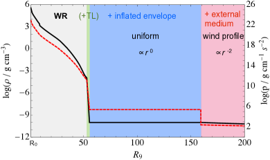
Figure 3: Rest-mass density (black solid) and pressure (red dashed) profiles of model 35OC (Woosley & Heger, 2006, the original star has a radius $R_{9}\simeq 52$), in addition to the inflated WR envelope (blue shaded background) and the wind-like external medium (pink shaded background). Between the WR stellar core and the inflated envelope there is a thin transition layer (TL; green shaded) set for numerical convenience.

3.2 Inflated envelope and external medium

Although the stellar-evolution calculations the model is based on (Woosley & Heger, 2006) include all important processes (e.g. rotation and magnetic fields), the approximations required for following the evolution during the hydrostatic phases entail limitations in several aspects. One of those is the mass loss due to the intense winds driven by radiation pressure common to high-mass stars, which modify the environment of the star and may generate inflated envelopes or, in the most extreme cases, generate dense shells around the star. Mass loss is included in the models in a parametrized way without accounting for the detailed structure of the stellar winds beyond the surface of the star. Consequently, we have to set the profiles of density and temperature outside the star in such a way that they are consistent both with typical mass loss rates of this class of stars and with the properties of the GRB/SN progenitors we want to model (see e.g. Crowther 2007). Recent studies (see, e.g. Gräfener, Owocki & Vink, 2012; Sanyal, Moriya & Langer, 2015) consider that, instead of a typical wind, WR stars may develop very dilute ‘inflated’ envelopes that can extend far beyond ($R_{\rm env}\sim 10^{12}$ cm) the location of the core ($R_{\rm c}\lesssim 10^{11}$) and increase the opacity, reconciling the large WR radii observed with the idea of compact WR cores as GRB progenitors. Based on this hypothesis, we consider that an inflated envelope with a uniform rest-mass density, $\rho_{\rm env}\gtrsim 10^{-10}\,$g cm^-3, and pressure, $p_{\rm env}\sim 10^{6}$ g cm^-1 s^-2, is generated at the surface of the WR (see e.g. Fig. 2 of Gräfener et al. 2012 for their most massive WR model of $23M_{\odot}$). This envelope is not contained in the stellar evolution model of Woosley & Heger (2006). With these values both the rest-mass density and pressure show strong jumps at the interface separating the WR star and the envelope. Thus, for reasons of numerical stability, we have implemented a transition layer consisting of 50 radial zones in the layer $[R_{\star},5.56\times 10^{10}\,{\rm cm}]$ to smoothly connect these two regions (Fig. 2). The radial extent of the inflated envelope, $\Delta R_{\mathrm{env}}:=R_{\rm env}-R_{\star}$, was found by Gräfener et al. (2012) to be a few stellar radii ($R_{\star}$), with higher values for higher stellar masses. Lacking detailed information for model 35OC, our choice of $\Delta R_{\mathrm{env}}=2R_{\star}\approx 1.1\times 10^{11}$ cm, is motivated by the fact that a much larger value would make the envelope optically thick, in conflict with the fact that stars that end as fast rotating WR stars may become transparent to UV radiation during the main-sequence evolution (Szécsi et al., 2015). From $R_{\rm env}$ outwards we assume that both rest-mass density and pressure follow a wind profile, i.e. $p$, $\rho\propto r^{-2}$. Immediately outside of $R_{\rm env}$, i.e. in the interface that separates the inflated envelope from the wind-like medium, we fix $\rho_{\rm EM,0}=\rho_{\rm env}$ and $p_{\rm EM,0}=2.5\times 10^{5}$ g cm^-1 s^-2. Though, the wind is moving with a subrelativistic speed away from the star and the envelope may be lossing mass, the speeds of both media are much smaller than those the jets we set up in Sec. 3.4 develop. Thus, in practice, we assume that both the wind-like medium and the envelope are at rest. For simplicity, hereafter we will refer to the wind-like external medium as just the external medium (EM).

3.3 SN ejecta

Detailed models of core collapse of the pre-supernova model 35OC (Obergaulinger & Aloy, 2017) show that a SN explosion may develop within less than a second after core bounce. While the shock wave propagates outwards, the conditions at the center might lead to the launching of a GRB jet after a further delay of the order of a few seconds (see further discussion in the next Section).

In order to incorporate in our model the dynamics generated by an on-going SN explosion, we inject in our stellar progenitor at $R_{\rm inj}(\emph{SN})=R_{0}$ a synthetic SN ejecta driven ad hoc by a piston-like mechanism (App. A). This injection radius has been chosen because it puts our inner boundary well outside the iron core and the surrounding matter that has fallen onto the hypermassive PNS by the time we start our simulations (see Obergaulinger & Aloy, 2017). We have simplified our set up reducing the SN ejecta propagation to a 1D, spherically symmetric problem. Certainly, we do not expect a SN shock launched in a fast rotating stellar progenitor (as the one at hand) to be perfectly isotropic, however, beyond the further simplified jet/SN ejecta interaction, the 1D ejecta modelling reduces considerably the computational cost associated to the calculation of its hydrodynamic evolution as it travels inside of the stellar envelope.

The initialization of the SN ejecta is done using a piston-like model similar to that of Rosenberg & Scheuer (1973) or Gull (1973), since energy, $E_{\rm SN}$, and mass, $M_{\rm SN}$, are carried by an spherical flow, which enters the numerical grid through the inner boundary, at a constant rate, until $t_{\rm SN}=1$ s (see, Tab. 1). The stellar potential sets a minimum required amount of energy to launch any outflow at a distance $R_{0}$. We have checked that the binding energy of the matter on the numerical domain is $\gtrsim 5\times 10^{50}$ erg, i.e. any successful SN must exceed this value, which is compatible with energies of typical SN. Thus, the total energy injected is $E_{\rm SN}=10^{52}\,$erg, which places this model in the HN realm (consistently with GRB/SN associations), while the total mass injected by the piston mechanism through the innermost radial boundary has been fixed to $M_{\rm SN}=0.1M_{\odot}$. This mass is removed from the excised mass enclosed below $R_{0}$. The reason for this operational procedure is to not modify the gravitational potential (and, hence, the equilibrium conditions) in the layers of the star beyond the SN shock. In case we do not apply this correction to $M_{\rm in}$, unwanted displacements of the outer progenitor mass shells (including the stellar surface) are generated (see App. B). Once the constant injection phase is over, a quickly decaying mass and energy injection follows. After that, the inner boundary is open and copy conditions are set, allowing the inflow of material from the grid to the excised part. During this phase, we follow the evolution of $M_{\rm in}$, which is suitably updated to self consistently compute the gravitational potential.

Table 1: Summary of some of the parameters of all models: dimensionality (Dim), true luminosity ($L$), isotropic equivalent energy ($E_{\rm iso}$), true energy ($E$), initial Lorentz factor ($\Gamma$), initial specific enthalpy ($h$), injection time ($t_{\rm inj}$), injection radius ($R_{\rm inj}$), inner mass below $R_{\rm inj}$ ($M_{\rm in}$) and time delay with respect to the SN ($t_{\rm del}$). The true luminosity corresponds to $E_{\rm SN}/t_{\rm inj}$ and to $L_{\rm j}$ for the SN and jet injection cases, respectively. $E_{\rm iso}$ is computed assuming that the half-opening angle at jet breakout of the stellar surface is approximately the same as that at injection ($\theta_{\rm BO}\simeq\theta_{\rm j}$).

Model	SN	J0a	J0b	J0c	J3a	J3b	J3c	J3d
Dim	1D	2D	2D	2D	2D	2D	2D	2D
$L$ (erg s-1)	$10^{52}$	$1.1\times 10^{49}$	$5.7\times 10^{48}$	$2.9\times 10^{48}$	$1.1\times 10^{49}$	$5.7\times 10^{48}$	$2.9\times 10^{48}$	$1.1\times 10^{48}$
$E_{\rm iso}$ (erg)	$10^{52}$	$10^{54}$	$5.0\times 10^{53}$	$2.5\times 10^{53}$	$10^{54}$	$5.0\times 10^{53}$	$2.5\times 10^{53}$	$10^{53}$
$E$ (erg)	$10^{52}$	$3\times 10^{50}$	$1.5\times 10^{50}$	$7.6\times 10^{49}$	$3\times 10^{50}$	$1.5\times 10^{50}$	$7.6\times 10^{49}$	$3\times 10^{49}$
$\Gamma$	$1.0315$	5	5	5	5	5	5	5
$h$	$1.0237$	20	20	20	20	20	20	20
$t_{\rm inj}$ (s)	1	20	20	20	20	20	20	20
$R_{\rm inj}$	$R_{0}$	$2R_{0}$	$2R_{0}$	$2R_{0}$	$2R_{0}$	$2R_{0}$	$2R_{0}$	$2R_{0}$
$M_{\rm in}$ ($M_{\odot}$)	$3.385$	$6.055$	$6.055$	$6.055$	$3.289$	$3.289$	$3.289$	$3.289$

3.4 Jets

The delay between a successful SN explosion and the subsequent generation of a relativistic jet from the central engine is not completely known. Thus, we discuss next several possibilities. Vietri & Stella (1998) formulated the so-called supranova model, which predicts the formation of a supramassive NS (SMNS), i.e. a NS stabilized by centrifugal forces at a mass exceeding the limit for non-rotating stars (Baumgarte et al., 2000). In the supranova model, the timescale of energy loss and subsequently collapse to BH for the SMNS is of the order of years, which seems to be in conflict with the nearly simultaneous observations of GRBs associated to SNe (see Königl 2004 and references therein). However, as pointed by Guetta & Granot (2003), the SN/GRB delay time may span a wide range of values, from near coincidence (similar to the collapsar model) to even years. This broad range of delays may reconcile the supranova model with SN/GRB almost simultaneous detections, as well as with cases in which a SN counterpart is not observed together with a GRB event (Woosley & Bloom, 2006).

Specifically for the model 35OC, the General Relativistic Hydrodynamic core-collapse simulations of O’Connor & Ott (2011) predict BH formation times after core bounce in the range $[0.84,2.7]\,$s, depending on the nuclear EoS considered. These calculations were done including a simplified neutrino leakage scheme, unable to drive a SN explosion. More recently, Obergaulinger & Aloy (2017), including a much more elaborated neutrino transport method and magnetic fields as indicated by stellar evolution calculations, find that the BH formation time after bounce can be larger than the upper bounds estimated in O’Connor & Ott (2011). In some models it is even likely that a BH does not form at all. In the cases in which the BH forms, it is necessary to wait a bit more until energy can be efficiently extracted from the central engine, since an accretion disc must be generated, which may take a few seconds after the BH is formed. Furthermore, the ram pressure of the accreting matter will be too high to allow for jet launching until the polar regions accrete so much mass that their density decreases below $\sim 10^{6}\,$g cm^-3 (MacFadyen & Woosley, 1999). Altogether, the time elapsed between core bounce and jet formation is an uncertain quantity on the order of several seconds, as long as or even above $\sim 5$–$10\,$s. In this work, we consider a time delay between the SN and the jet of $t_{\rm del}=3$ s. For comparison, we note that the SN shock of model 35OC-RO of Obergaulinger & Aloy (2017) has already reached $\simeq 3\times 10^{9}\,$cm at $1.6$ s after the core of model 35OC bounces, which is before BH formation.

We assume that a relativistic jet has been already formed inside our inner boundary, which is shifted to $R_{\rm inj}(\emph{Jet})=2R_{0}$ in the second (2D) step of our simulations (see Sec. 3). We note that the injection radius of the jet and of the 1D SN ejecta differ. We inject a conical flow through the innermost boundary of our computational domain in the medium left behind by the SN ejecta. During the 1D step of our models, the SN ejecta crosses $R_{\rm inj}(\emph{Jet})$ after $\Delta t_{\rm SN}\simeq 0.8$ s from its numerical injection (deeper inside the star, at $R_{\rm inj}(\emph{SN})$). Furthermore, we let it evolve for another period of time equal to $t_{\rm del}$ inside the computational grid until it is sufficiently far from the jet injection nozzle. Then we map the rest-mass density, pressure and radial velocity profiles of the 1D SN ejecta evolution as initial conditions for the simulations with jets (models J3) and remap them into a new 2D spherical grid. All in all, the SN ejecta has been travelling outwards for a time $\Delta t_{\rm SN}+t_{\rm del}\simeq 3.8\,$s before the beginning of the 2D step of our simulations. As a calibration, we also consider the case in which no ejecta have not been injected previously (model J0).

The SN ejecta reduces the enclosed mass below the jet injection boundary since, (1) it injects a mass $M_{\rm SN}$, which we assume is extracted from the excised region below $R_{\rm inj}(\emph{SN})$, and (2) it plows part of the stellar mass in the region between $R_{0}$ and $2R_{0}$. Therefore, in models J3 the inner mass enclosed below $R_{\rm inj,j}$ is reduced to $M_{\rm in}\text{(J3)}\simeq M_{\rm in}-M_{\rm SN}\approx 3.289M_{\odot}$.

We have set isotropic equivalent energies of $E_{\rm iso,j}=10^{54}\,$erg (models J0a and J3a) and $5\times 10^{53}$ erg (model J3b). From Fig. 1, we see the largest of the latter values roughly corresponds to the threshold energy for model 35OC at $R_{\rm inj,j}$. Imposing that the half-opening angle of the jet be $\theta_{\rm j}=2^{\circ}$, the true jet energies become $E_{\rm j}=(1-\cos{\theta_{\rm j}})/2\times E_{\rm iso,j}\simeq 3\times 10^{50}$ erg (J0a and J3a) and $1.5\times 10^{50}$ erg (J3b). The jets are injected for $t_{\rm inj,j}=20$ s, so that their isotropic luminosities are $L_{\rm iso,j}=3.8\times 10^{52}\,$erg s^-1 (J0a and J3a) and $1.9\times 10^{52}\,$erg s^-1 (J3b) and the true luminosities are $L_{\rm j}\simeq 1.1\times 10^{49}$ erg s^-1 (J0 and J3a) and $5.7\times 10^{48}$ erg s^-1 (J3b). In all the models the initial jet Lorentz factor $\Gamma_{\rm j}=5$ and specific enthalpy $h_{\rm j}=20$ translate into an asymptotic Lorentz factor $\Gamma_{\infty,0}=h_{\rm j}\Gamma_{\rm j}=100$. See a summary of the parameters of each model in Tab. 1.

We point out that Nagakura et al. (2011) have also studied how the earlier emergence of a shock can influence the propagation (and emission) of a jet. In the work of Nagakura et al. an ongoing shock arises naturally after gravitational collapse is stalled in the star envelope by the effect of centrifugal forces (i.e. it is not the SN shock resulting from the core collapse, which in Nagakura et al.’s model is assumed to have been swallowed by the central BH). Furthermore, we note, that the progenitor model employed in Nagakura et al. (2011) is not directly a progenitor resulting from a stellar-evolution code. Instead, the authors build their own rotating equilibrium configuration to closely mimic the density distribution of model 16TI from Woosley & Heger (2006). This model corresponds to a metal poor star that has a ZAMS mass of $16M_{\odot}$, and rotates rapidly.

4 Simulations

In this section we show and discuss the results of the numerical simulations employed to assess the analytic luminosity threshold found in Sec. 2. We have run two series of jet models with different energies at the injection point: (1) the J0 series, in which no SN ejecta was injected previously, and (2) the J3 series, in which it was. We have checked whether jets with luminosities close to the threshold set by Eq. (6) are able to break out the progenitor star, at least in a time $t\lesssim t_{\rm inj,j}$.

Figure 4 shows those models which break out the star in a time $t<t_{\rm inj,j}$. They correspond to the jet models J0a and J3a and J3b. We note that model J0a possesses an intrinsic luminosity slightly above $L_{\rm j}^{\rm thr}$. This is also the case of models J3a and, especially, of J3b, whose luminosity threshold is smaller than for model J0a because of the action of the SN ejecta (compare the blue and magenta lines in Fig.1). In all these models, the jet remains well collimated from the injection until they break out of the surface of the star. Indeed, the jets of models J3a and J3b have overtaken the SN forward shock (FS) wave, as can be seen in the mid and right panels of Fig. 4. After an initial transient phase (following the jet breakout) in which $\theta_{\rm BO}$ cannot be reliably estimated, the jet opening angle decreases and settles to a value $\sim 9^{\circ}-11^{\circ}$ in all jet cases (Fig. 5). These values are $\gtrsim 5\theta_{j}$, i.e., substantially larger than the initial opening angle of the jet. We note that in Fig. 5, the time range is limited to be of the order of $t_{\rm inj}$. After that time the injection luminosity quickly declines and the measurement of $\theta_{\rm BO}$ is polluted by the fact that the beam of the jet becomes only mildly relativistic. The monotonical increase observed, e.g., in model J3b $\sim 20\,$s post-breakout is, thereby, an artifact resulting from the operative criterion employed to measure it.

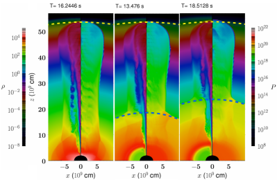
Figure 4: Snapshots of rest-mass density (left side of each panel) and pressure (right side of each panel) in the laboratory frame of models J0 (left panel), J3a (central panel) and J3b (right panel) at breakout from the stellar surface (times are annotated above each panel). The rest-mass density (palette on the left side of the figure) and pressure (palette on the right side of the figure) are in CGS units. $R_{\star}$ and the radius, $R_{\rm FS,SN}$, reached by the SN forward shock (FS) are marked with yellow and blue dashed lines, respectively. (the time since injection is written above each panel)

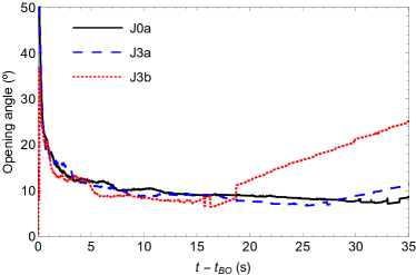
Figure 5: Time evolution, in the laboratory frame, of the opening angle of the jet after breakout of the surface of the star for models J0a (black solid), J3a (blue dashed) and J3b (red dotted). The practical measurement of $\theta_{\rm BO}$ is rather involved around the time when the jets breakout and, therefore, the left part of the plot until $t-t_{\rm BO}\sim 2\,$s does not represent the actual jet half-opening angle, but instead, the jet’s forward shock angular extension. Models J0b, J0c, J3c and J3d are not show in the figure for different reasons. Model J0b displays a cocoon breakout and its beam does not emerge out of the stellar surface, hence we cannot reliably measure $\theta_{\rm BO}$. Model J0c does not even enter successfully the grid. Model J3c displays a very quick lateral expansion by the time it arrives to the stellar surface and the values of $\theta_{\rm BO}$ cannot be measured accurately (but they are much larger than those of model J0a). Model J3d is chocked in the SN ejecta and it does not properly breakout.

Three snapshots of the evolution of model J0b, with an injection luminosity $\sim 2$ times below the threshold of Eq. (6) are shown in Fig. 6. In this case, the jet is successfully injected in the computational grid, but it develops a large, quasi-spherical, subrelativistic cocoon within the star and it is much less collimated than the most luminous model of the J0 series. Moreover, the beam of the jet remains trapped by the thick cocoon surrounding it. Instead of a jet breakout, we find a cocoon breakout from the stellar surface, which happens at a time $t\sim 57\text{\,s}\,>t_{\rm inj,j}$ and traps the jet itself. We have checked that for the jet model J0c, with a luminosity $\sim 4$ times below $L_{\rm j}^{\rm thr}$, injection directly fails and the jet does not even progress inside the computational grid. From the exploration of the J0 series of models we find that model J0b is a borderline case between successful jet injection and jet injection failure.

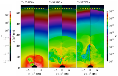
Figure 6: Snapshots of the evolution of model J0b. The quantities displayed are the same as in Fig. 4. Note that depicted times are all longer than $t_{\rm inj,j}=20$ s (the time since injection is written above each panel).

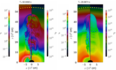
Figure 7: Snapshots of the evolution of models J3d (left panel) and J3c (right panel). The quantities displayed are the same as in Fig. 4, but the color scales of the left panel are different for better visualization. On the left panel the FS of the SN ejecta is already outside the represented length. Note that depicted times are different and longer than $t_{\rm inj,j}=20$ s (the time since injection is written above each panel).

In addition to the fact that the passage of the SN ejecta may lower the pressure and the rest-mass density in the vicinity of the jet injection nozzle, it also drives a radial outward motion of the stellar matter with a subrelativistic speed $v_{\rm r,a}$. If $v_{\rm r,a}\sim v_{\rm h}$, the value of $L_{\rm j}^{\rm thr}$ may be further decreased, since the ram pressure on the jet’s head is significantly reduced. Thus, we have considered two additional members of the J3 series with luminosities 4 (J3c) and 10 (J3d) times than the luminosity threshold found for the reference model J0a (Tab. 1), slightly below the threshold predicted analytically for the J3 series of models (Fig. 1; magenta line). The model J3c, hosting an equivalent isotropic energy twice smaller than $E_{\rm iso}^{\rm thr}(\text{J3b})$ at $R_{9}=2$, breaks of out the star, but after a time $t\sim 3t_{\rm inj,j}$ (Fig. 7; right panel). On the other hand, in the model J3d, with $E_{\rm iso}=10^{53}$ erg (a factor of 5 less than $E_{\rm iso}^{\rm thr}(\text{J3})$) the SN ejecta breaks out the star before the jet does it (Fig. 7; left panel). In fact, the jet of model J3d is trapped within the SN ejecta and fails to catch up with them because the latter propagates faster once they enters the EM.

5 Discussion and conclusions

Aiming to explore the dynamics of relativistic jets, which may result into events compatible with the phenomenology of llGRBs and GRB-SNe, we have studied both analytically and numerically the conditions under which low-luminosity jets may break out of a potential stellar progenitor of the former type of events. In order for a jet, i.e. a supersonic flow to form at a pre-stablished injection nozzle, the luminosity must be above a certain threshold depending on the conditions within the progenitor at the injection point. In order to assess the influence of the progenitor conditions several considerations follow. The collapse of the inner core of low metallicity, fast-rotating, massive stars may produce the conditions to generate the central engine of a GRB as well as a successful SN explosion. Our numerical models are set up assuming that unspecified processes (e.g. magnetohydrodynamic stresses or neutrino heating) have generated collimated outflows inside the core of the collapsed star. The propagation of a SN shock produces a drastic change in the structure of the star undergoing the SN explosion. As the SN ejecta sweep the stellar mantle, they modify the medium in which a GRB jet, produced by the central engine, shall propagate. We have justified that the delay between the generation of the SN ejecta and the trailing GRB jet should probably be of, at most, a few seconds on the basis of theoretical models and recent simulations of the formation of the central engine of GRBs. Obergaulinger & Aloy (2017) show that a SN explosion may develop within less than a second after core bounce. While the shock wave propagates outwards, the conditions at the center might lead to the launching of a GRB jet after a further delay of the order of a few seconds. However, since we expect the GRB jet to be substantially faster than the SN ejecta, the former will eventually catch up the later, drill its way trough the expanding SN shocked layer and proceed later through the rest of the stellar progenitor (unless the jet/SN ejecta interaction catastrophically hinders the ulterior jet propagation).

In this paper, we have also assessed the existence of the aforementioned theoretical luminosity threshold by means of multi-dimensional, special relativistic, hydrodynamics simulations. Our jets are injected at the polar axis through the inner radial boundary situated at $R_{\rm inj,j}=2\times 10^{9}\,\mathrm{cm}$ with a half-opening angle of $\theta_{\rm j}=2^{\circ}$. Jets with smaller injection half-opening angles are hardly compatible with hydrodynamic or MHD generation and collimation processes. Jets with larger injection half-opening angles are endowed with larger luminosities in our model set up, and thus, they are very far from the conditions expected to generate llGRBs. Two of our jet models (J0a and J3b) have been chosen with luminosities only a bit above to threshold at $R_{9}=2$ in the pre-supernova model 35OC while others (J0b, J0c, J3c and J3d) fall below the aforementioned luminosity threshold. We have found numerically that jets with luminosities below the threshold of Eq. (7) failed in breaking out of the star.

Beyond the theoretical point that insufficiently powerful jets fail to even travel through the stellar mantle, the foremost relevant point is addressing how the intrinsic jet luminosity thresholds we have obtained translate into thresholds in the equivalent isotropic luminosity of the jets and, hence, on the expected $L_{\rm\gamma,iso}$. In order to translate the intrinsic jet luminosities at the jet injection point into equivalent isotropic quantities it is necessary, first of all, a reliable estimation of the outflow opening angle after the jet breaks out of the surface of the star. Two basic possibilites have been considered: either the jet opening angle is basically the same as the initial jet opening angle or much larger than that. The former alternative follows from the results of Mizuta & Ioka (2013). The latter from our own results. Assuming that the outflow opening angle remains as small as $\theta_{j}$, models J0a and J3a would have $E_{\rm iso,j}=10^{54}$ erg ($L_{\rm iso,j}=5\times 10^{52}$ erg s^-1), while model J3b would yield $E_{\rm iso,j}=5\times 10^{53}$ erg ($L_{\rm iso,j}=2.5\times 10^{52}$ erg s^-1). We have tried to push down the previous values to bring them as close as possible to the observed range in llGRBs ($L_{\rm\gamma,iso}\sim 10^{46}$–$10^{48}$ erg), but values below 2-3 times $10^{51}\,$erg s^-1 are unattainable if we aim to launch a jet that is not choked inside of the star (Fig. 1) in the typically assumed progenitors of llGRBs. We must bear in mind that the hydrodynamic isotropic luminosities do not directly correspond to the $\gamma$- and/or X-ray radiation, since part of this energy may be still stored in the form of a thermal energy reservoir that can be released on longer time scales, over lower observational frequencies (e.g., in the radio band) or converted to kinetic energy of the outflow. Moreover, part of the injected energy can be dissipated by its interaction in the progenitor. Following the arguments of Mizuta & Ioka (2013), the energies considered here would need a tiny efficiency factor for conversion of hydrodynamic energy into radiation, $\epsilon_{\gamma}\lesssim 10^{-5}$, to lie in the llGRB regime.

Our models show that jets develop opening angles after breakout $\theta_{\rm BO}\gg\theta_{j}=2^{\circ}$, so that the luminosity condition relaxes to Eq. (10) (in that equation we assumed $a\sim 3$). This conclusion is in contrast with the findings of Mizuta & Ioka (2013), but does not necessarily contradict the results of the latter authors, since, our setup is different from that of Mizuta & Ioka in many aspects. For instance, we employ model 35OC as stellar progenitor, which is more extended and massive than model 16TI employed by the former authors. We consider much lower luminosity jets ($L_{\rm j}\gtrsim 1.5\times 10^{49}$ erg s^-1) than Mizuta & Ioka (who use $L_{\rm j}=10^{50}$ erg s^-1). We inject jets with an asymptotic Lorentz factor $\Gamma_{\infty,0}=100$, while Mizuta & Ioka (2013) use a much larger value ($\simeq 538$). Another differences are the jet injection angle and time. Mizuta & Ioka (2013) use $\theta_{\rm j}\simeq 4.6^{\circ}$, and $t_{\rm inj,j}=12.5$ s, while we use $\theta_{\rm j}\simeq 2^{\circ}$, and $t_{\rm inj,j}=20$ s. Finally, the inference of the former authors on the jet opening angle is not time independent. $\theta_{\rm BO}$ could depend on the setup of the circumburst medium. As can be seen from their Fig. 9, there is some trend for the jet breakout angle to increase with time. Due to the larger values of $\theta_{\rm BO}$ of our models, jets with the same injection luminosities as we have set up produce lower equivalent isotropic luminosities than in Mizuta & Ioka. This means that, efficiencies of $\epsilon_{\gamma}\sim 1\%$ could give rise to $\gamma$-ray luminosities in the range observed for the llGRB population in our jet models.

The duration of jet injection is a free parameter of our simulations. It has been set to $t_{\rm inj,j}=20$ s, which is more typical for standard long GRBs rather than for llGRBs, which show durations from hundreds to thousands of seconds. However, the existence of an injection luminosity threshold is independent of the duration of the energy injection. Noteworthy, the breakout times of those models with $L_{\rm j}\gtrsim L_{\rm j}^{\rm thr}$ (especially the one measured for model J3b, $t_{\rm BO}\text{(J3b)}=18.51$ s) are close to the injection time (i.e. $t_{\rm BO}\lesssim t_{\rm inj,j}$). Bromberg et al. (2011a) suggested that jets with $t_{\rm BO}>t_{\rm inj,j}$ would fail in breaking out of the star as they would be choked by the stellar envelope. We have examples of jets with $t_{\rm BO}>t_{\rm inj,j}$ (e.g. J3c) that still can break out of its progenitor star. However, we do not expect such jets to produce very luminous events since the jet/SN ejecta interaction is strong and may dissipate a large fraction of the jet internal energy. In any case, the estimated analytical threshold for well posed jet injection is related with the breakout time. Precisely, we find $t_{\rm BO}>t_{\rm inj,j}$ when $L_{\rm j}$ is a factor $\sim 2$ smaller than $L_{\rm j}^{\rm thr}$. Furthermore, we find that jets with an intrinsic luminosity smaller than $\sim L_{\rm j}^{\rm thr}/4$ get trapped within the stellar progenitor or within the SN ejecta, and that jets with $L_{\rm j}\lesssim L_{\rm j}^{\rm thr}/5$ are not even properly injected in the numerical grid.

Remarkably, we have found with our numerical tests that the simple analytic estimate for $L_{\rm j}^{\rm thr}$ over-predicts the existence of a luminosity threshold by a factor $\sim 2-3$. The analytic estimate is more accurate for models without a SN ejecta perturbing the stellar structure. This is expected, since we have neglected the motion of the ambient medium to estimate it, and the SN ejecta drives the stellar layers close to the jet injection nozzle radially outward, which reduces the ram pressure on the head of the jet. In our models without a SN ejecta the analytic threshold is still a bit larger than found numerically. This likely due to the fact that we have neglected the gravitational pull in the estimation of the jet’s head velocity. For powerful relativistic jets, the latter assumption is well justified. In our case, with weaker relativistic jets, whose head moves only slightly supersonically with respect to the stellar medium, the accuracy of the forme assumption is not as good. Over and above all these considerations, it remains true that our estimated $L_{\rm j}^{\rm thr}$ is a good proxy for the minium hydrodynamic luminosity attainable by relativistic jets successfully propagating inside likely progenitors of llGRBs.

Finally, we point out that the existence of luminosity thresholds for the injection of a jet (based upon the necessity of producing a supersonic outflow) is not restricted to the specific context we have addressed here. The arguments employed to derive $L_{\rm j}^{\rm thr}$, also hold qualitatively in other scenarios. Among them, we outline the injection of low luminosity jets in the remnant left behind the merger of neutron stars. In full analogy with our findings in the present paper, this criterion should be used in combination with the standard assumption that the jet injection time must be sufficiently long for the jet to break out of the merger ejecta (Moharana & Piran, 2017). We defer for a future work exploring this possibility.

Appendix A The ‘piston’ model

The 1D SN ejecta is injected from the start of the simulation until a final time of $t_{\rm SN}$ with a piston-like model in which we set both the energy and the mass fluxes, $\dot{E}_{\rm SN}=E_{\rm SN}/t_{\rm SN}$ and $\dot{M}_{\rm SN}=M_{\rm SN}/t_{\rm SN}$ respectively, across the innermost radius of our computational domain, $R_{0}$. After $t_{\rm SN}$, the energy and mass injection are not switch off abruptly but decay very rapidly with time ($\propto t^{-12}$). This fast injection decline is introduced for numerical convenience, since the gas behind the rear end of the SN ejecta is very rarefied. The gradient of, e.g. density between ejecta and the trailing matter is very steep for an instantaneous end of the injection, which can cause a failure of the simulation. This instability can be removed by a smooth transition at the end of the SN injection. The steep time decrease of the ejecta injection conditions has been tuned to keep injecting a negligible amount of energy and mass in the computational grid on the time scales of interest (a few seconds).

Taking units in which $c=1$, the injection model is based upon the main assumption that $\Theta:=p/\rho\ll 1$ (where $p$ and $\rho$ are the fluid pressure and density). This holds as long as $E_{\rm SN}\ll M_{\rm SN}c^{2}$, condition we guarantee setting up suitable values for the parameters $E_{\rm SN}$ and $M_{\rm SN}$. Using the TM EoS (Mignone & McKinney, 2007), the square of the speed of sound, $c_{\rm s}$, is

$$c_{\rm s}^{2}=\frac{\Theta}{3h}\frac{5h-8\Theta}{h-\Theta}\approx\frac{5\Theta}{3h}\,,$$ (12)

and the specific enthalpy is

$$h=\frac{5}{2}\Theta+\sqrt{\frac{9}{4}\Theta^{2}+1}\approx\frac{5}{2}\Theta+1\,,$$ (13)

where the last approximate expressions in Eqs. (12) and (13) hold for $\Theta\ll 1$.

From the energy and mass flux we get that

$$\xi:=h\Gamma=1+\frac{\dot{E}_{\rm SN}}{\dot{M}_{\rm SN}c^{2}}\,.$$ (14)

Using the definition of the Mach number, $\mathcal{M}=v/c_{\rm s}$, with $\beta$ the (radial) velocity of the fluid, the bulk Lorentz factor takes the form

$$\Gamma=1/\sqrt{1-\mathcal{M}^{2}c_{s}^{2}}\,.$$ (15)

Using Eqs. (12)–(15), we arrive at

$$\Theta=\frac{6(\xi^{2}-1)}{45+\xi^{2}(10\mathcal{M}^{2}-15)}\,,$$ (16)

which only depends on the parameters $\dot{E}_{\rm SN}$, $\dot{M}_{\rm SN}$ and $\mathcal{M}$ and will always be much smaller than 1 for the typical parameters of our SN ejecta set up. The Mach number is set to ensure that the shock is supersonic at injection, $\mathcal{M}=2$.

Once $\Theta$ is computed we recover in the following order, $h$ (Eq. (13)), $\Gamma=\xi/h$ (Eq. (14)), $\rho$ (from the mass flux) and $p=\Theta\rho$. Note that $\xi\geq h$ must be fulfilled in order to assure that $\Gamma\geq 1$, i.e. it will be satisfied that

$$\Theta\leq\frac{2}{5}(\xi-1)\,.$$ (17)

Appendix B Gravitational potential

The equations of relativistic hydrodynamics in axial symmetry, employing spherical coordinates, $\textbf{x}=$($r$, $\theta$), natural units ($c=G=1$) and neglecting the fluid’s self-gravity are (e.g. Cuesta-Martínez, 2017):

$$\frac{\partial\textbf{U}}{\partial t}+\frac{1}{r^{2}}\frac{\partial r^{2}\textbf{F}}{\partial r}+\frac{1}{r\sin\theta}\frac{\partial\sin\theta\textbf{G}}{\partial\theta}=\mathbf{S_{\mathbf{U}}}.$$ (18)

The vector of conserved quantities, U, and the $r$- and $\theta$- components of the momentum, F and G respectively, are defined as

U $$=\begin{pmatrix}D\\ S^{r}\\ S^{\theta}\\ \tau\end{pmatrix},$$ (19)

F $$=\begin{pmatrix}Dv^{r}\\ S^{r}v^{r}+p\\ S^{\theta}v^{r}\\ (\tau+p)v^{r}\end{pmatrix}\>\mbox{and}$$ (20)

G $$=\begin{pmatrix}Dv^{\theta}\\ S^{r}v^{\theta}\\ S^{\theta}v^{\theta}+p\\ (\tau+p)v^{\theta}\end{pmatrix},$$ (21)

where $D$, $\textbf{S}=(S^{r},S^{\theta})$ and $\tau$ are the relativistic mass density, the momentum density and the energy density, respectively, all of them measured in the laboratory frame and defined as a function of the primitive variables:

$$D =\rho\Gamma,$$ (22)

S $$=\rho h\Gamma^{2}\textbf{v},$$ (23)

$$\tau =\rho h\Gamma^{2}-p-D.$$ (24)

The velocity is also measured in the laboratory frame, $\textbf{v}=(v^{r},v^{\theta})$, and relates to the four-velocity as

$$u^{\mu}=\Gamma(1,\textbf{v}),$$ (25)

where

$$\Gamma\equiv\frac{1}{\sqrt{1-\textbf{v}^{2}}}$$ (26)

is the fluid (bulk) Lorentz factor. We note that the components of both momentum density and velocity are expressed in orthonormal spherical basis.

In the absence of physical sources, the source term, $\mathbf{S_{\mathbf{U}}}$, only contains all the geometrical factors in 2D spherical coordinates:

$$\mathbf{S_{\mathbf{U}}}=\displaystyle\frac{1}{r}\begin{pmatrix}0\\ 2p+S^{\theta}v^{\theta}\\[3.0pt] \displaystyle\frac{\cos\theta}{\sin\theta}p-S^{\theta}v^{r}\\ 0\end{pmatrix}.$$ (27)

Gravitational effects may become relevant if the deeper regions of the star are included in the model. Nevertheless, in order to reach hydrostatic equilibrium in the star, we need to introduce self-gravity for balancing the pressure gradient, particularly at the stellar surface. This is especially true if the time over which we compute the models is comparable or larger than the sound crossing time of the stellar radius.

We have included in MRGENESIS a Newtonian gravitational potential, $\Phi$, in order to account for self-gravity. Although our code is relativistic, we have chosen a Newtonian potential for simplicity, but including some relativistic corrections as considering in the source term $\rho_{\rm eff}:=(\rho h\Gamma^{2}-p)$ instead of $\rho_{\rm eff}:=\rho$ alone. We note that a similar approach has been followed by Nagakura et al. (2011). Since we do not account for general relativity effects, the metric remains unchanged and, therefore, the influence of the potential only appears as an additional source term in the equations of the RHD (18). The new source term reads $\textbf{S}_{\rm new}=\textbf{S}_{\textbf{U}}+\textbf{S}_{\rm pot}$, where $\textbf{S}_{\textbf{U}}$ is defined in Eq. (27) and $\textbf{S}_{\rm pot}$ denotes the source vector due to the inclusion of the Newtonian potential. In 2D spherical coordinates:

$$\textbf{S}_{\rm pot}=\begin{pmatrix}0\\ \\ -(\rho h\Gamma^{2}-p)\displaystyle{\frac{\partial\Phi}{\partial r}}\\ \\ -\displaystyle{\frac{1}{r}}(\rho h\Gamma^{2}+S^{r}v^{r})\displaystyle{\frac{\partial\Phi}{\partial\theta}}\\ \\ -\rho h\Gamma^{2}\left(v^{r}\displaystyle{\frac{\partial\Phi}{\partial r}}+\displaystyle{\frac{v^{\theta}}{r}}\displaystyle{\frac{\partial\Phi}{\partial\theta}}\right)\end{pmatrix},$$ (28)

Once the potential source term is volume-averaged, we get

$$\tilde{\textbf{S}}_{\rm pot}:=\frac{1}{\Delta V}\int\limits_{V}\textbf{S}_{\rm pot}\text{ d}V=\begin{pmatrix}0\\ \\ -(\rho_{i,j}h_{i,j}\Gamma_{i,j}^{2}-p_{i,j})\,S^{r}_{0,\rm pot}\\ \\ -(\rho_{i,j}h_{i,j}\Gamma_{i,j}^{2}+S_{i,j}^{r}v_{i,j}^{r})\,S^{\theta}_{0,\rm pot}\\ \\ -\rho_{i,j}h_{i,j}\Gamma_{i,j}^{2}\,(v_{i,j}^{r}S^{r}_{0,\rm pot}+v_{i,j}^{\theta}S^{\theta}_{0,\rm pot})\end{pmatrix},$$ (29)

being

$$\begin{split}S^{r}_{0,\rm pot}=&\frac{3}{\Delta r^{3}}\Big{[}\Phi_{i+1/2,j}r_{i+1/2}^{2}-\Phi_{i-1/2,j}r_{i-1/2}^{2}-\Phi_{i,j}\Delta r^{2}\Big{]}\\ S^{\theta}_{0,\rm pot}=&-\frac{3}{2}\frac{\Delta r^{2}}{\Delta r^{3}\Delta\cos{\theta}}\times\\ &\Big{[}\Phi_{i,j+1/2}\sin{\theta_{j+1/2}}-\Phi_{i,j-1/2}\sin{\theta_{j-1/2}}-\\ &\>\Phi_{i,j}\Delta\sin{\theta}\Big{]},\end{split}$$ (30)

where in a given cell $(i,j)$ the potential has to be known also at the cell boundaries $i+1/2$, $i-1/2$, $j+1/2$ and $j-1/2$. In the previous expression we have introduced the notation, $\Delta r^{2}:=r_{i+1/2}^{2}-r_{i-1/2}^{2}$, $\Delta r^{3}:=r_{i+1/2}^{3}-r_{i-1/2}^{3}$, $\Delta\cos{\theta}:=\cos{\theta_{j+1/2}}-\cos{\theta_{j-1/2}}$ and $\Delta\sin{\theta}:=\sin{\theta_{j+1/2}}-\sin{\theta_{j-1/2}}$.

For uniformly spaced grids we make the simple assumption that

$$\Phi_{i+1/2,j} =\frac{1}{2}(\Phi_{i+1,j}+\Phi_{i,j})$$ (31)

$$\Phi_{i+1/2,j} =\frac{1}{2}(\Phi_{i,j}+\Phi_{i-1,j}).$$ (32)

and the same is done for the interface values in the $j$-direction.

The Poisson equation,

$$\Delta\Phi=4\pi\rho_{\rm eff}$$ (33)

defines the behaviour of the potential, $\Phi$, and its dependence on the mass distribution. To find the solution of this elliptic equation, we have used the method devised in Adsuara et al. (2016, 2017). For numerical convenience, we do not solve directly for the potential $\Phi=\Phi(r,\theta)$ but a modified potential $\Phi^{\prime}(r,\theta)=\Phi(r,\theta)+M_{\rm in}/r$, where $M_{\rm in}$ is the excised mass below $R_{0}$. Neumann conditions for the potential are imposed at $R_{0}$, $\frac{\partial\Phi^{\prime}}{\partial r}|_{R_{0}}=0$, and Dirichlet conditions at the outer end of the radial grid, $\Phi^{\prime}(R_{f},\theta)=-M_{T}/R_{f}$. The total mass within the grid, $M_{T}$, excludes the excised mass $M_{\rm in}$. Once $\Phi^{\prime}$ is calculated, we only have to subtract in the radial direction the quantity $M_{\rm in}/r$ to recover the real potential, $\Phi$.

The potential is recalculated after a number of iterations equal to multiples of the number of cells in the radial direction, $n_{r}$. The reason is that $n_{r}\Delta t$ corresponds to the light crossing time in the grid and the potential is updated before any perturbation can cross the whole numerical grid. Between two consecutive calculations it is very likely that the inner mass has changed due to a non-zero mass flux across $R_{0}$ (interface $1/2$). This flux can supply a non-negligible amount of mass to the enclosed mass $M_{\rm in}$, making it necessary to consider it in order to properly recompute the potential. Whether or not such a contribution is included can strongly influence the dynamics, specially in those regions close to $R_{\rm inj,j}$. The total incoming mass, calculated as $\Delta M_{\rm in}=-\sum_{j}F_{1/2,j}S_{1/2,j}$, is evaluated in every time step in the same manner as for the conserved variables, i.e. it is updated in each of the Runge-Kutta steps of our time integration method. In the latter formula $F_{1/2,j}$ is the mass flux per unit surface between cells $(0,j)$ and $(1,j)$ and $S_{1/2,j}=4\pi(-\Delta\cos\theta)R_{\rm inj,j}^{2}$ is the surface of the respective boundary located at $R_{\rm inj,j}$. After the end of the time loop $\Delta M_{\rm in}$ is removed from the grid and incorporated to the inner mass.

References

- Adsuara et al. (2016) Adsuara J. E., Cordero-Carrión I., Cerdá-Durán P., Aloy M. A., 2016, Journal of Computational Physics, 321, 369
- Adsuara et al. (2017) Adsuara J. E., Cordero-Carrión I., Cerdá-Durán P., Mewes V., Aloy M. A., 2017, Journal of Computational Physics, 332, 446
- Aloy et al. (1999) Aloy M. A., Ibáñez J. M., Martí J. M., Müller E., 1999, ApJS, 122, 151
- Aloy et al. (2000) Aloy M. A., Müller E., Ibáñez J. M., Martí J. M., MacFadyen A., 2000, ApJ, 531, L119
- Baumgarte et al. (2000) Baumgarte T. W., Shapiro S. L., Shibata M., 2000, ApJ, 528, L29
- Bromberg & Tchekhovskoy (2016) Bromberg O., Tchekhovskoy A., 2016, MNRAS, 456, 1739
- Bromberg et al. (2011a) Bromberg O., Nakar E., Piran T., 2011a, ApJ, 739, L55
- Bromberg et al. (2011b) Bromberg O., Nakar E., Piran T., Sari R., 2011b, ApJ, 740, 100
- Bufano et al. (2012) Bufano F., et al., 2012, ApJ, 753, 67
- Campana et al. (2006) Campana S., et al., 2006, Nature, 442, 1008
- Cano et al. (2011) Cano Z., et al., 2011, ApJ, 740, 41
- Cano et al. (2015) Cano Z., et al., 2015, MNRAS, 452, 1535
- Cano et al. (2017) Cano Z., Wang S.-Q., Dai Z.-G., Wu X.-F., 2017, Advances in Astronomy, 2017, 8929054
- Cerdá-Durán et al. (2013) Cerdá-Durán P., DeBrye N., Aloy M. A., Font J. A., Obergaulinger M., 2013, ApJ, 779, L18
- Cobb et al. (2006) Cobb B. E., Bailyn C. D., van Dokkum P. G., Natarajan P., 2006, ApJ, 645, L113
- Colella & Woodward (1984) Colella P., Woodward P. R., 1984, Journal of Computational Physics, 54, 174
- Coward (2005) Coward D. M., 2005, MNRAS, 360, L77
- Crowther (2007) Crowther P. A., 2007, ARA&A, 45, 177
- Cuesta-Martínez (2017) Cuesta-Martínez C., 2017, PhD thesis, Departamento de Astronomía y Astrofísica, Universidad de Valencia, Spain
- Fan et al. (2011) Fan Y.-Z., Zhang B.-B., Xu D., Liang E.-W., Zhang B., 2011, ApJ, 726, 32
- Galama et al. (1998) Galama T. J., et al., 1998, Nature, 395, 670
- Gräfener et al. (2012) Gräfener G., Owocki S. P., Vink J. S., 2012, A&A, 538, A40
- Guetta & Della Valle (2007) Guetta D., Della Valle M., 2007, ApJ, 657, L73
- Guetta & Granot (2003) Guetta D., Granot J., 2003, MNRAS, 340, 115
- Gull (1973) Gull S. F., 1973, MNRAS, 161, 47
- Hjorth (2013) Hjorth J., 2013, Philosophical Transactions of the Royal Society of London Series A, 371, 20120275
- Hjorth et al. (2003) Hjorth J., et al., 2003, Nature, 423, 847
- Irwin & Chevalier (2016) Irwin C. M., Chevalier R. A., 2016, MNRAS, 460, 1680
- Ito et al. (2015) Ito H., Matsumoto J., Nagataki S., Warren D. C., Barkov M. V., 2015, ApJ, 814, L29
- Iwamoto et al. (1998) Iwamoto K., et al., 1998, Nature, 395, 672
- Königl (2004) Königl A., 2004, in Feroci M., Frontera F., Masetti N., Piro L., eds, Astronomical Society of the Pacific Conference Series Vol. 312, Gamma-Ray Bursts in the Afterglow Era. p. 333 (arXiv:astro-ph/0302110)
- Kumar & Zhang (2015) Kumar P., Zhang B., 2015, Phys. Rep., 561, 1
- Lazzati & Begelman (2010) Lazzati D., Begelman M. C., 2010, ApJ, 725, 1137
- Lazzati et al. (2009) Lazzati D., Morsony B. J., Begelman M. C., 2009, ApJ, 700, L47
- Lazzati et al. (2013) Lazzati D., Morsony B. J., Margutti R., Begelman M. C., 2013, ApJ, 765, 103
- Leismann et al. (2005) Leismann T., Antón L., Aloy M. A., Müller E., Martí J. M., Miralles J. A., Ibáñez J. M., 2005, A&A, 436, 503
- Liang et al. (2007) Liang E., Zhang B., Virgili F., Dai Z. G., 2007, ApJ, 662, 1111
- López-Cámara et al. (2013) López-Cámara D., Morsony B. J., Begelman M. C., Lazzati D., 2013, ApJ, 767, 19
- López-Cámara et al. (2014) López-Cámara D., Morsony B. J., Lazzati D., 2014, MNRAS, 442, 2202
- López-Cámara et al. (2016) López-Cámara D., Lazzati D., Morsony B. J., 2016, ApJ, 826, 180
- MacFadyen & Woosley (1999) MacFadyen A. I., Woosley S. E., 1999, ApJ, 524, 262
- MacFadyen et al. (2001) MacFadyen A. I., Woosley S. E., Heger A., 2001, ApJ, 550, 410
- Malesani et al. (2004) Malesani D., et al., 2004, ApJ, 609, L5
- Martí et al. (1997) Martí J. M., Müller E., Font J. A., Ibáñez J. M. Z., Marquina A., 1997, ApJ, 479, 151
- Matzner (2003) Matzner C. D., 2003, MNRAS, 345, 575
- Mignone & McKinney (2007) Mignone A., McKinney J. C., 2007, MNRAS, 378, 1118
- Mignone et al. (2005) Mignone A., Plewa T., Bodo G., 2005, ApJS, 160, 199
- Mimica et al. (2009) Mimica P., Aloy M.-A., Agudo I., Martí J. M., Gómez J. L., Miralles J. A., 2009, ApJ, 696, 1142
- Mizuta & Aloy (2009) Mizuta A., Aloy M. A., 2009, ApJ, 699, 1261
- Mizuta & Ioka (2013) Mizuta A., Ioka K., 2013, ApJ, 777, 162
- Mizuta et al. (2006) Mizuta A., Yamasaki T., Nagataki S., Mineshige S., 2006, ApJ, 651, 960
- Modjaz et al. (2016) Modjaz M., Liu Y. Q., Bianco F. B., Graur O., 2016, ApJ, 832, 108
- Moharana & Piran (2017) Moharana R., Piran T., 2017, MNRAS, 472, L55
- Morsony et al. (2007) Morsony B. J., Lazzati D., Begelman M. C., 2007, ApJ, 665, 569
- Morsony et al. (2010) Morsony B. J., Lazzati D., Begelman M. C., 2010, ApJ, 723, 267
- Nagakura et al. (2011) Nagakura H., Ito H., Kiuchi K., Yamada S., 2011, ApJ, 731, 80
- Nakar (2015) Nakar E., 2015, ApJ, 807, 172
- Nakar & Sari (2012) Nakar E., Sari R., 2012, ApJ, 747, 88
- O’Connor & Ott (2011) O’Connor E., Ott C. D., 2011, ApJ, 730, 70
- Obergaulinger & Aloy (2017) Obergaulinger M., Aloy M., 2017, MNRAS, 469, L43
- Paczyński (1998) Paczyński B., 1998, ApJ, 494, L45
- Page et al. (2011) Page K. L., et al., 2011, MNRAS, 416, 2078
- Patat et al. (2001) Patat F., et al., 2001, ApJ, 555, 900
- Pian et al. (2006) Pian E., et al., 2006, Nature, 442, 1011
- Rosenberg & Scheuer (1973) Rosenberg I., Scheuer P. A. G., 1973, MNRAS, 161, 27
- Sanyal et al. (2015) Sanyal D., Moriya T. J., Langer N., 2015, in Hamann W.-R., Sander A., Todt H., eds, Wolf-Rayet Stars: Proceedings of an International Workshop held in Potsdam, Germany, 1-5 June 2015. Edited by Wolf-Rainer Hamann, Andreas Sander, Helge Todt. Universitätsverlag Potsdam, 2015., p.213-216. pp 213–216 (arXiv:1508.06055)
- Shibata et al. (2000) Shibata M., Baumgarte T. W., Shapiro S. L., 2000, Phys. Rev. D, 61, 044012
- Singer et al. (2015) Singer L. P., et al., 2015, ApJ, 806, 52
- Soderberg et al. (2006) Soderberg A. M., et al., 2006, Nature, 442, 1014
- Soderberg et al. (2008) Soderberg A. M., et al., 2008, Nature, 453, 469
- Stanek et al. (2003) Stanek K. Z., et al., 2003, ApJ, 591, L17
- Starling et al. (2011) Starling R. L. C., et al., 2011, MNRAS, 411, 2792
- Szécsi et al. (2015) Szécsi D., Langer N., Yoon S.-C., Sanyal D., de Mink S., Evans C. J., Dermine T., 2015, A&A, 581, A15
- Vietri & Stella (1998) Vietri M., Stella L., 1998, ApJ, 507, L45
- Waxman et al. (2007) Waxman E., Mészáros P., Campana S., 2007, ApJ, 667, 351
- Woosley (1993) Woosley S. E., 1993, ApJ, 405, 273
- Woosley & Bloom (2006) Woosley S. E., Bloom J. S., 2006, ARA&A, 44, 507
- Woosley & Heger (2006) Woosley S. E., Heger A., 2006, ApJ, 637, 914
- Zhang et al. (2003) Zhang W., Woosley S. E., MacFadyen A. I., 2003, ApJ, 586, 356
- Zhang et al. (2004) Zhang W., Woosley S. E., Heger A., 2004, ApJ, 608, 365