Fluid and gyrofluid modeling of low-$\beta_{e}$ plasmas:
phenomenology of kinetic Alfvén wave turbulence

Abstract

Reduced fluid models including electron inertia and ion finite Larmor radius corrections are derived asymptotically, both from fluid basic equations and from a gyrofluid model. They apply to collisionless plasmas with small ion-to-electron equilibrium temperature ratio and low $\beta_{e}$, where $\beta_{e}$ indicates the ratio between the equilibrium electron pressure and the magnetic pressure exerted by a strong, constant and uniform magnetic guide field. The consistency between the fluid and gyrofluid approaches is ensured when choosing ion closure relations prescribed by the underlying ordering. A two-field reduction of the gyrofluid model valid for arbitrary equilibrium temperature ratio is also introduced, and is shown to have a noncanonical Hamiltonian structure. This model provides a convenient framework for studying kinetic Alfvén wave turbulence, from MHD to sub-$d_{e}$ scales (where $d_{e}$ holds for the electron skin depth). Magnetic energy spectra are phenomenologically determined within energy and generalized helicity cascades in the perpendicular spectral plane. Arguments based on absolute statistical equilibria are used to predict the direction of the transfers, pointing out that, within the sub-ion range associated with a $k_{\perp}^{-7/3}$ transverse magnetic spectrum, the generalized helicity could display an inverse cascade if injected at small scales, for example by reconnection processes.

I Introduction

Reduced fluid models including electron inertia are classically used to study collisionless magnetic reconnection. These models, which are limited to scales large with respect to the electron Larmor radius $\rho_{e}$, require a small value of the electron beta parameter $\beta_{e}$ defined as the ratio between the equilibrium electron pressure and the magnetic pressure exerted by a strong, constant and uniform magnetic guide field. Similarly, at the level of the ions, a fluid computation of ion finite Larmor radius (FLR) corrections restricts the considered scales to be either much larger than the ion Larmor radius $\rho_{i}$ (for which a perturbative approach is possible) or much smaller than $\rho_{i}$, a case studied in Ref. Passot et al. (2017), where the ion velocity is negligible. Denoting with $\tau$ a constant equilibrium ion-to-electron temperature ratio, when concentrating on scales of the order of the sonic Larmor radius $\rho_{s}$, defined as $\rho_{s}=\rho_{i}/\sqrt{2\tau}$, these regimes correspond to a value of $\tau$ much smaller or much larger than unity, respectively. In the case where magnetic fluctuations along the guide field are retained, the case of negligible $\tau$ was addressed in two dimensions in Refs. Fitzpatrick and Porcelli (2004, 2007) and extended to three dimensions in Ref. Tassi et al. (2010). The case where $\tau$ is small but not totally negligible (or finite, provided the considered scales are assumed larger than $\rho_{i}$) was addressed in Ref. Hsu et al. (1986), when electron inertia is neglected. One of the motivations of the present paper is to extend this four-field model by retaining electron inertia, using a rigorous asymptotic ordering. Such a small-$\tau$ asymptotics, performed at scales of the order of the sonic Larmor radius $\rho_{s}$, involves a second order computation of the ion FLR corrections in terms of $k_{\perp}\rho_{i}$, where $k_{\perp}$ refers to the transverse wavenumber of the fluctuations. As will be shown, the resulting reduced fluid model can also be obtained as an asymptotic limit of the gyrofluid model derived in Ref. Brizard (1992). The question then arises of the consistency of the two approaches, an issue which may be sensitive to the closure assumptions. The case of finite $\tau$ can be addressed using a gyrofluid approach which, retaining the parallel magnetic fluctuations $B_{z}$, remains valid for somewhat larger values of $\beta_{e}$, at least at large enough scales. When reduced to two fields by neglecting the coupling to the parallel ion velocity $u_{i}$ and thus to the slow magneto-acoustic modes, the resulting gyrofluid model isolates the dynamics of kinetic Alfvén waves (KAWs) which are supposed to play a main role in the solar wind.

Another aim of this paper is to use this two-field gyrofluid model to study phenomenologically critically-balanced KAW turbulence at scales ranging from MHD to sub-$d_{e}$ scales (where $d_{e}$ stands for the electron skin depth), paying a special attention to the transverse magnetic energy spectra in the energy or the generalized helicity cascades, and to the direct or inverse character of these cascades. Such Kolmogorov-like phenomenology dismisses the possible effect of coherent structures such as current sheets which form as the result of the turbulent MHD cascade and which, in some instances, can be destabilized by magnetic reconnection. Recent two-dimensional hybrid-kinetic simulations Cerri and Califano (2017) suggest that, in the non-collisional regime, this process is fast enough to compete with the wave mode interactions, in a way that could affect the cascade at scales comparable to the ion inertial length $d_{i}$, typical of the current sheet width. In a small $\beta_{i}$ plasma, where $\beta_{i}=\tau\beta_{e}$, this scale is significantly larger than $\rho_{s}$, and the spectral break can indeed take place at $d_{i}$, as suggested by recent two-dimensional hybrid simulations Franci et al. (2016). The above gyrofluid model can provide an efficient tool to address this issue.

At this point, it is useful to order the various relevant scales estimated in a homogeneous equilibrium state characterized by a density $n_{0}$, isotropic ion and electron temperatures $T_{0i}$ and $T_{0e}$, and subject to a strong ambient magnetic field of amplitude $B_{0}$ along the $z$-direction. In terms of the sonic Larmor radius $\rho_{s}=c_{s}/\Omega_{i}$, where $c_{s}=\sqrt{T_{0e}/m_{i}}$ is the sound speed and $\Omega_{i}=eB_{0}/(mc)$ the ion gyrofrequency, one has

$$d_{i}=\sqrt{\frac{2}{\beta_{e}}}\rho_{s},\qquad d_{e}=\sqrt{\frac{2}{\beta_{e}}}\delta\rho_{s},$$

$$\rho_{i}=\sqrt{2\tau}\rho_{s},\qquad\rho_{e}=\sqrt{2}\delta\rho_{s},$$ (1)

where $\beta_{e}=8\pi n_{0}T_{0e}/B_{0}^{2}$, $\delta^{2}=m_{e}/m_{i}$ is the electron to ion mass ratio and $\tau=T_{0i}/T_{0e}$. We have here defined the particle Larmor radii ($r=i$ for the ions, $r=e$ for the electrons) by $\rho_{r}=v_{th\,r}/\Omega_{r}$ where the particle thermal velocities are given by $v_{th\,r}=(2T_{r}/m_{r})^{1/2}$ and the inertial lengths by $d_{r}=v_{A}/\Omega_{r}$ where $v_{A}=B_{0}/(4\pi n_{0}m_{i})^{1/2}=c_{s}\sqrt{2/\beta_{e}}$ is the Alfvén velocity.

The models to be derived should cover a spectral range which includes both scales large compared to $d_{i}$ (typical of the width of the generated current sheets) and scales comparable to $d_{e}$ (typical of collisionless reconnection processes). The considered scales will also be assumed to remain large compared to $\rho_{e}$, so that electron FLR corrections reduce to the contribution ensuring the gyroviscous cancellation. This in particular implies the condition that $\rho_{e}/d_{e}=\beta_{e}^{1/2}$ be small enough.

On the other side, the ion to electron temperature ratio $\tau$ determines the magnitude of $\rho_{i}$ relatively to the considered scales. If $\tau\gg 1$, they are much smaller than $\rho_{i}$, which makes ion velocities negligible. This case can be addressed using a fluid model, as shown in Ref. Passot et al. (2017). For $\tau\ll 1$, they are much larger than $\rho_{i}$, and the problem is also amenable to a fluid approach with ion FLR corrections estimated perturbatively. This regime is addressed in Section II. For intermediate values of $\tau$, a gyrofluid approach is required. It is the object of Section III. In Section IV, a two-fluid restriction of this model is used for a phenomenological study of critically-balanced kinetic Alfvén wave (KAW) turbulence. Section V presents a short summary together with a few comments.

II Fluid modeling for small $\tau$

Two regimes will be here considered with $\beta_{e}$ scaling either like $\delta$ (scaling I) or like $\delta^{2}$ (scaling II). The value of $\tau$ must then be chosen so that $\rho_{i}$ be small enough compared to $\rho_{s}$ (taken as the characteristic scale), but also smaller than $d_{e}$. Since $\rho_{i}/\rho_{s}=(2\tau)^{1/2}$ and $\rho_{i}/d_{e}=(\tau\beta_{e})^{1/2}/\delta$, one should take $\tau=O(\delta^{3/2})$ for scaling I and $\tau=O(\delta)$ for scaling II. In the case of scaling I $d_{i}/\rho_{s}\simeq\rho_{s}/d_{e}\simeq d_{e}/\rho_{e}\simeq 1/\delta^{1/2}$, and $d_{e}/\rho_{i}\simeq 1/\delta^{1/4}$, whereas for scaling II, $d_{e}$ and $\rho_{s}$ are comparable and clearly separated from $d_{i}$ (by a factor $1/\delta$) and $\rho_{i}$ (by a factor $1/\delta^{1/2}$).

It is convenient to take the sonic Larmor radius $\rho_{s}$, the sound speed $c_{s}$ and the inverse ion gyrofrequency $\Omega_{i}^{-1}$ as length, velocity and time units. Using the same nondimensional units as in Ref. Tassi et al. (2016), the amplitude of the fluctuations of density $n$ and of the electric potential $\varphi$ are controlled by the parameter $\varepsilon\ll 1$, as $n\sim\varphi=O(\varepsilon)$. We assume that at scale $\rho_{s}$, $\partial_{t}=O(\varepsilon)$ and $\mathbf{\nabla}_{\perp}\sim O(1)$. We denote by $A_{\|}$ the parallel component of the magnetic potential, by $u_{i}$ and $u_{e}$ the parallel ion and electron velocity respectively and by $B_{z}$ the longitudinal magnetic field fluctuations. In the case of scaling I, $A_{\|}\sim u_{i}\sim\partial_{z}=O(\varepsilon\delta^{1/2})$, $u_{e}=O(\varepsilon/\delta^{1/2})$, and $B_{z}=O(\varepsilon\delta)$ (thus to be retained). Differently, for scaling II, $A_{\|}\sim u_{i}\sim\partial_{z}=O(\varepsilon\delta)$, $u_{e}=O(\varepsilon/\delta)$, and $B_{z}=O(\varepsilon\delta^{2})$ (thus negligible). We furthermore denote by ${\mathbf{P}}_{r}$ the pressure tensor of the $r$ particle species, given by the sum of a gyrotropic part involving the parallel and perpendicular pressure fluctuations $p_{\|r}$ and $p_{\perp r}$ and of a non-gyrotropic contribution ${\boldsymbol{\Pi}}_{r}$. Such scalings lead to the derivation of reduced fluid models retaining corrections $O(\tau)$ or $O(\delta)$, relatively to the leading order.

The Ampère equation reads

$$\Delta_{\perp}A_{\|}=\frac{\beta_{e}}{2}(u_{e}-u_{i}).$$ (2)

Summing the equations satisfied by the ion and electron velocities ${\boldsymbol{u}}_{i}$ and ${\boldsymbol{u}}_{e}$ leads to

$$(1+n)\{\partial_{t}\left({\boldsymbol{u}_{i}}+\delta^{2}{\boldsymbol{u}_{e}}\right)+{\boldsymbol{u}}_{i}\mathbf{\cdot}\mathbf{\nabla}_{\perp}{\boldsymbol{u}_{i}}+\delta^{2}{\boldsymbol{u}}_{e}\mathbf{\cdot}\mathbf{\nabla}_{\perp}{\boldsymbol{u}_{e}}\}$$

$$\qquad+\mathbf{\nabla}_{\perp}\mathbf{\cdot}\Big{(}\tau{\mathbf{P}}_{i}+{\mathbf{P}}_{e}\Big{)}-\frac{2}{\beta_{e}}{\boldsymbol{J}}{\boldsymbol{\times}}{\boldsymbol{B}}=0,$$ (3)

which, in the small-amplitude (weakly nonlinear) and quasi-transverse asymptotics, gives

$$\frac{d^{i}}{dt}u_{i}+\delta^{2}\frac{d^{e}}{dt}u_{e}+\nabla_{\|}(\tau p_{\|i}+p_{\|e})+\tau{\widehat{\boldsymbol{b}}}\mathbf{\cdot}\mathbf{\nabla}\cdot{\boldsymbol{\Pi}}_{i}+{\widehat{\boldsymbol{b}}}\mathbf{\cdot}\mathbf{\nabla}\cdot{\boldsymbol{\Pi}}_{e}=0$$ (4)

for the parallel components. Here, we introduced the parallel derivative $\nabla_{\|}f={\widehat{\boldsymbol{b}}}\mathbf{\cdot}\mathbf{\nabla}f=-[A_{\|},f]+\partial_{z}f$, with $[f,g]={\widehat{\boldsymbol{z}}}\mathbf{\cdot}(\mathbf{\nabla}f\times\mathbf{\nabla}g)=\partial_{x}f\partial_{y}g-\partial_{y}f\partial_{x}g$, where $f$ and $g$ refer to scalar functions, and ${\widehat{\boldsymbol{z}}}$ to the unit vector along the guide field. Noting that, to leading order,

$${\widehat{\boldsymbol{b}}}\mathbf{\cdot}\mathbf{\nabla}_{\perp}{\boldsymbol{\times}}({\boldsymbol{J}}{\boldsymbol{\times}}{\boldsymbol{B}})=\nabla_{\|}J_{\|}=-\nabla_{\|}\Delta_{\perp}A_{\|},$$ (5)

one also gets

$$\frac{d^{i}}{dt}\Delta_{\perp}\varphi_{i}+\delta^{2}\frac{d^{e}}{dt}\Delta_{\perp}\varphi_{e}+{\widehat{\boldsymbol{b}}}\cdot\mathbf{\nabla}_{\perp}\times\mathbf{\nabla}_{\perp}\cdot(\tau{\mathbf{P}}_{i}+{\mathbf{P}}_{e})$$

$$+\frac{2}{\beta_{e}}\nabla_{\|}\Delta_{\perp}A_{\|}=0$$ (6)

for the sum of the ion and electron vorticities. Here ${\widehat{\boldsymbol{b}}}$ is the unit vector along the local magnetic field and the convective time derivative $d^{r}/dt$ stands for $\partial_{t}+[\varphi_{r},\cdot]$, where the potentials $\varphi_{r}$ of the leading order transverse velocities of the r-particle species (${\boldsymbol{u}}_{\perp r}={\widehat{\boldsymbol{b}}}\times\mathbf{\nabla}\varphi_{r}$), are given by $\varphi_{i}=\varphi+\tau p_{\perp i}-({\tau}/{2})\Delta_{\perp}\varphi_{i}$ and $\varphi_{e}=\varphi-p_{\perp e}-({\delta^{2}}/{2})\Delta_{\perp}\varphi_{e}$. In these formulas, the first term is associated with the so-called ${\boldsymbol{E}}\times{\boldsymbol{B}}$ drift, the second one to the diamagnetic drift, while the last one originates from the leading order non-gyrotropic pressure contribution. Here and in the rest of the paper, electrons will be taken isothermal, leading to $p_{\|e}=p_{\perp e}=n$.

The equations for the magnetic potential and for the parallel magnetic field component are easily obtained (see Ref. Passot et al. (2017)) as

$$\partial_{t}(A_{\|}-\delta^{2}u_{e})+\nabla_{\|}(\varphi-n)-\delta^{2}[\varphi_{e},u_{e}]-{\widehat{\boldsymbol{b}}}\cdot\mathbf{\nabla}\cdot{\boldsymbol{\Pi}}_{e}=0$$

(7)

$$\frac{d^{e}}{dt}(B_{z}-n-\delta^{2}\Delta_{\perp}\varphi_{e})-\nabla_{\|}u_{e}-{\widehat{\boldsymbol{b}}}\cdot\mathbf{\nabla}_{\perp}\times\mathbf{\nabla}_{\perp}\cdot(\frac{{\boldsymbol{\Pi}}_{e}}{1+n})=0.$$

The system of governing equations is supplemented by the perpendicular pressure balance, obtained by taking the transverse divergence of the transverse component of Eq. (3) considered to leading order,

$$\frac{2}{\beta_{e}}B_{z}=\frac{\tau}{2}\Delta_{\perp}\varphi_{i}-\tau p_{\perp i}-n.$$ (9)

II.1 The case of negligible ion temperature

In the case of scaling I, the system made up of Eqs. (2), (4), (6)-(9) greatly simplifies as all the non-gyrotropic pressure components become sub-dominant, except the electronic ones associated with the gyroviscous cancellation. The $\tau$ contributions also drop out, and we obtain, writing $\frac{d}{dt}=\partial_{t}+[\varphi,\mathbf{\cdot}]$,

$$\frac{d}{dt}(1+\frac{2}{\beta_{e}})B_{z}-\nabla_{\|}u_{e}=0$$ (10)

$$\frac{d}{dt}(A_{\|}-\delta^{2}u_{e})+\partial_{z}\varphi+\frac{2}{\beta_{e}}\nabla_{\|}B_{z}=0$$ (11)

$$\frac{d}{dt}(u_{i}+\delta^{2}u_{e})-\frac{2}{\beta_{e}}\nabla_{\|}B_{z}=0$$ (12)

$$\frac{d}{dt}\Delta_{\perp}\varphi+\frac{2}{\beta_{e}}\nabla_{\|}\Delta_{\perp}A_{\|}=0$$ (13)

$$u_{e}-u_{i}=\frac{2}{\beta_{e}}\Delta_{\perp}A_{\|},$$ (14)

which is a 3D extension of the model presented in Ref. Comisso et al. (2012), when taken in the cold-ion limit. Note that in this system, $B_{z}=-(\beta_{e}/2)n$. As mentioned in Ref. Comisso et al. (2012), it is easy to verify that, up to terms of order $\delta^{2}$, and after a simple rescaling, these equations also identify, in the 2D case, to those of Refs. Fitzpatrick and Porcelli (2004, 2007). A 3D extension of the latter model was given in Ref. Tassi et al. (2010). Both systems possess a Hamiltonian formulation, with the same Poisson bracket structure. In particular, in the 2D limit, they both possess four infinite families of Casimir invariants, three of which associated with Lagrangian invariants.

When writing the above system using the Alfvén velocity instead of the ion sound speed as velocity unit (i.e. substituting $u_{i}=\sqrt{2/\beta_{e}}u_{i}^{\prime}$, $\varphi=\sqrt{2/\beta_{e}}\varphi^{\prime}$, $\partial_{t}=\sqrt{2/\beta_{e}}\partial_{t}^{\prime}$) and neglecting the electron inertia, we recover the reduced Hall-magnetohydrodynamics (RHMHD) equations (E19) and (E20) of Ref. Schekochihin et al. (2009). Furthermore, as noted in Ref. Boldyrev et al. (2015), when concentrating on Alfvén waves and thus neglecting the coupling to $u_{i}$, one easily checks that, in the present low $\beta_{e}$ limit where the coefficient $1+2/\beta_{e}$ in Eq. (10) reduces to $2/\beta_{e}$, the $\beta_{e}$ parameter can be scaled out by writing $B_{z}=\sqrt{\beta_{e}/2}B_{z}^{\prime}$, thus making $\rho_{s}$ the only characteristic scale of this system.

When neglecting electron inertia, Eqs. (10)-(14) can be considered for any value of $\beta_{e}$. In the large $\beta_{e}$ limit and in 2D, by using the above rescalings for $u_{i}$, $\varphi$ and time, the resulting system identifies with Eqs. (20)-(23) of Ref. Andrés et al. (2014) for incompressible two-fluid MHD, when taking $\varepsilon=\sqrt{2/\beta_{e}}$ which measures $d_{i}$ in units of $\rho_{s}$. Note that the system derived in Ref. Andrés et al. (2014) involves an equation for $A_{z}$ instead of $A_{\|}$ (quantities which identify at the considered order). In this case, the last term of Eqs. (11) originates from the Hall term, while it here results from the electron pressure in Ohm’s law. Pressure balance ensures the equality of these two contributions.

II.2 The case of small but finite ion temperature

II.2.1 Derivation of the ion FLR contributions

Since with scaling II, $\rho_{i}/\rho_{s}=O(\delta^{1/2})$, ion FLR corrections enter the dynamics as contributions of order $\delta$. Using this scaling, we first derive the electron equations. At the required order in Eq. (II), we have $\varphi_{e}=\varphi-n$ and, from Ref.Passot et al. (2017),

$${\widehat{\boldsymbol{b}}}\mathbf{\cdot}(\mathbf{\nabla}_{\perp}\mathbf{\cdot}{\boldsymbol{\Pi}}_{e})=\delta^{2}[n,u_{e}].$$ (15)

This contribution cancels the diamagnetic drift $\delta^{2}[n,u_{e}]$ that originates from the second term of $\varphi_{e}$. Equation (II) thus rewrites

$$\frac{d}{dt}(A_{\|}-\delta^{2}u_{e})+\partial_{z}\varphi-\nabla_{\|}n=0.$$ (16)

In Eq. (II), $B_{z}$ is negligible as well as the non-gyrotropic pressure contribution. This equation thus reduces to

$$\frac{d}{dt}n+\nabla_{\|}u_{e}=0.$$ (17)

We now turn to the velocity equations (4) and (6). The ion non-gyrotropic pressure tensor can be estimated within a perturbative computation in terms of the parameters $\varepsilon$ and $\tau$ from the coupled system provided by Eq. (A6) of Ref. Schekochihin et al. (2010) and a drift expansion of the ion transverse velocity. Neglecting the heat flux contributions to ${\boldsymbol{\Pi}}_{i}$, we are led, in practice, to repeat the calculations made in Appendix A of Ref. Passot et al. (2017), only replacing pressures and velocities of the electrons by those of the ions and dropping the factors $-\delta^{2}$ and $\delta^{4}$, which corresponds to changing the charge and the mass when replacing electrons by ions. This results in expressing the parallel component of the nongyrotropic ion pressure force as

$${\widehat{\boldsymbol{b}}}\mathbf{\cdot}(\mathbf{\nabla}_{\perp}\mathbf{\cdot}{\boldsymbol{\Pi}}_{i})=-[p_{\perp i}-B_{z},u_{i}]-\nabla_{\|}\Delta_{\perp}\varphi_{i}$$

$$\qquad-[\mathbf{\nabla}_{\perp}\varphi_{i};\mathbf{\nabla}_{\perp}A_{\|}]-\partial_{t}\Delta_{\perp}u_{i}-[\varphi_{i},\Delta_{\perp}u_{i}]$$

$$\qquad+\frac{1}{2}[\Delta_{\perp}\varphi_{i},u_{i}]-[\mathbf{\nabla}_{\perp}\varphi_{i};\mathbf{\nabla}_{\perp}u_{i}],$$ (18)

where we use the notation $\displaystyle{[\mathbf{\nabla}f;\mathbf{\nabla}g]=\sum_{i}[\partial_{i}f,\partial_{i}g]}$. Equation (4) then rewrites

$$\partial_{t}(u_{i}-\tau\Delta_{\perp}u_{i}+\delta^{2}u_{e})+[\varphi_{i},u_{i}-\tau\Delta_{\perp}u_{i}]+[\varphi,\delta^{2}u_{e}]$$

$$\qquad-\tau[p_{\perp i}-\frac{1}{2}\Delta_{\perp}\varphi_{i},u_{i}]-\tau[\mathbf{\nabla}_{\perp}\varphi_{i};\mathbf{\nabla}_{\perp}(A_{\|}+u_{i})]$$

$$\qquad+\nabla_{\|}(n+\tau p_{\|i}-\tau\Delta_{\perp}\varphi_{i})=0.$$ (19)

For the vorticity equation, we need to express

$${\widehat{\boldsymbol{b}}}\mathbf{\cdot}\mathbf{\nabla}_{\perp}\times(\mathbf{\nabla}_{\perp}\mathbf{\cdot}{\boldsymbol{\Pi}}_{i})=-[p_{\perp i},\Delta_{\perp}\varphi_{i}]-[\mathbf{\nabla}_{\perp}p_{\perp i};\mathbf{\nabla}_{\perp}\varphi_{i}]$$

$$+\frac{1}{2}\nabla_{\|}\Delta_{\perp}u_{i}+\frac{1}{2}[\Delta_{\perp}A_{\|},u_{i}]+\frac{1}{2}\Delta_{\perp}(\mathbf{\nabla}\mathbf{\cdot}{\boldsymbol{u}}_{i})$$

$$-\frac{1}{4}\left(\partial_{t}\Delta_{\perp}^{2}\varphi_{i}+[\varphi_{i},\Delta_{\perp}^{2}\varphi_{i}]\right)-[\mathbf{\nabla}_{\perp}\varphi_{i};\mathbf{\nabla}_{\perp}\Delta_{\perp}\varphi_{i}],$$ (20)

where the last line of Eq. (20) is obtained by a computation to second order in terms of scale separation. The latter computation is rather cumbersome and was performed using MAPLE symbolic calculation software. In this expression, it is of interest to rewrite

$$\Delta_{\perp}(\mathbf{\nabla}\mathbf{\cdot}{\boldsymbol{u}}_{i})=-\Delta_{\perp}(\partial_{t}n+[\varphi_{i},n])=-\partial_{t}\Delta_{\perp}n$$

$$\quad-[\varphi_{i},\Delta_{\perp}n]-[\Delta_{\perp}\varphi_{i},n]-2[\mathbf{\nabla}_{\perp}\varphi_{i};\mathbf{\nabla}_{\perp}n],$$ (21)

where one can make the replacement

$$\partial_{t}\Delta_{\perp}n=-\Delta_{\perp}\left([\varphi_{i}+\frac{\tau}{2}\Delta_{\perp}\textperiodcentered\varphi_{i},n]+\nabla_{\|}u_{e}\right),$$ (22)

the second term in the bracket becoming subdominant when substituted into the vorticity equation.

At the considered order, noting that the contribution of the ion gyrotropic pressure is of lower order, the vorticity equation becomes, after writing $p_{\perp i}=n+t_{\perp i}$, where $t_{\perp i}$ refers to the perpendicular ion temperature fluctuations (and $t_{\|i}$ to the parallel ones),

$$\partial_{t}\left(\Delta_{\perp}\varphi_{i}-\frac{\tau}{4}\Delta_{\perp}^{2}\varphi_{i}\right)+[\varphi_{i},\Delta_{\perp}\varphi_{i}-\frac{\tau}{4}\Delta_{\perp}^{2}\varphi_{i}]$$

$$+\frac{2}{\beta_{e}}\nabla_{\|}\Delta_{\perp}A_{\|}+\frac{\tau}{2}\Delta_{\perp}\nabla_{\|}u_{e}+\tau[\Delta_{\perp}\varphi_{i},n]$$

$$+\tau[\mathbf{\nabla}_{\perp}\varphi_{i};\mathbf{\nabla}_{\perp}(n-\Delta_{\perp}\varphi_{i})]-\tau\mathbf{\nabla}_{\perp}\mathbf{\cdot}[t_{\perp_{i}},\mathbf{\nabla}_{\perp}\varphi_{i}]=0.$$

Determination of the temperature fluctuations: As discussed in Appendix A, the present scaling suggests considering an adiabatic regime for the ions, where gyrotropic heat fluxes are negligible. In this case, neglecting also the fourth-rank cumulant contributions ($B_{z}$ being small in the present ordering), one has

$$\frac{d^{i}}{dt}t_{\parallel_{i}}+2\nabla_{\|}u_{i}+\tau[t_{\parallel_{i}},p_{\perp i}]=0$$ (24)

or

$$\frac{d}{dt}t_{\parallel_{i}}-\frac{\tau}{2}[\Delta_{\perp}\varphi,t_{\parallel_{i}}]+2\nabla_{\|}u_{i}=0.$$ (25)

Similarly,

$$\frac{d^{i}}{dt}(t_{\perp_{i}}-n)-\nabla_{\|}u_{i}+2\tau[t_{\perp_{i}},p_{\perp i}]=0,$$ (26)

which rewrites

$$\frac{d}{dt}(t_{\perp_{i}}-n)-\frac{\tau}{2}[\Delta_{\perp}\varphi,t_{\perp_{i}}-n]-\nabla_{\|}u_{i}=0.$$ (27)

The terms of the form $\nabla_{\|}u_{i}$ are subdominant within scaling II. If one is not interested in the own dynamics of the temperatures, they only need to be determined at the dominant order, and it is possible to take

$$\frac{d}{dt}t_{\parallel_{i}}=0$$ (28)

$$\frac{d}{dt}t_{\perp_{i}}=\frac{d}{dt}n=-\nabla_{\|}u_{e}.$$ (29)

Since we also have

$$\Delta_{\perp}A_{\|}=\frac{\beta_{e}}{2}u_{e},$$ (30)

we conclude that, within scaling II, the equation for $u_{i}$ is decoupled. The system of Eqs. (II.2.1), (16), (17), together with (30), (29) and the relation $\varphi=\varphi_{i}+\frac{\tau}{2}\Delta_{\perp}\varphi_{i}-\tau n-\tau t_{\perp_{i}}$, conserves the energy

$${\mathcal{E}_{1}} = \frac{1}{2}\int\Big{(}|\mathbf{\nabla}_{\perp}\varphi_{i}|^{2}+\delta^{2}u_{e}^{2}+\frac{\tau}{4}(\Delta_{\perp}\varphi_{i})^{2}$$ (31)

$$+ \frac{2}{\beta_{e}}|\mathbf{\nabla}_{\perp}A_{\|}|^{2}+(1+\tau)n^{2}+\tau t_{\perp_{i}}^{2}\Big{)}d^{3}{\boldsymbol{x}}.$$

A further simplification is possible (with a proper choice of initial conditions) where temperatures are determined algebraically. For this purpose, one can remark that the number density $n$ is also given by the ion continuity equation in the form (after using the expression for $\varphi_{i}$)

$$\frac{dn}{dt}-\frac{\tau}{2}[\Delta_{\perp}\varphi,n]+\tau[p_{\perp i},n]+\mathbf{\nabla}\cdot{\boldsymbol{u}}_{i}=0.$$ (32)

In order to estimate $\mathbf{\nabla}_{\perp}\cdot{\boldsymbol{u}}_{\perp i}$, we consider the drift expansion of the transverse velocity.

$${\boldsymbol{u}}_{\perp i} = \frac{1}{B}{\widehat{\boldsymbol{b}}}\times\Big{\{}\mathbf{\nabla}_{\perp}\varphi+\frac{\tau}{1+n}\mathbf{\nabla}_{\perp}p_{\perp i}+\frac{\tau}{1+n}(\mathbf{\nabla}_{\perp}\mathbf{\cdot}{\boldsymbol{\Pi}}_{i})$$ (33)

$$+ \partial_{t}{\boldsymbol{A}}_{\perp}+\frac{d^{(i)}}{dt}{\boldsymbol{u}}_{\perp i}\Big{\}}.$$

where $B=|{\boldsymbol{B}}|=1+B_{z}+O(\varepsilon^{2})$ and ${\boldsymbol{A}}_{\perp}$ is the transverse component of magnetic vector potential. As at scales comparable to $\rho_{s}$, $B_{z}=O(\varepsilon\beta_{e})$ and ${\boldsymbol{A}}_{\perp}$ also scales as $\varepsilon\beta_{e}$, it follows that

$${\widehat{\boldsymbol{b}}}\times\frac{d^{(i)}}{dt}{\boldsymbol{u}}_{\perp i}=-\partial_{t}\mathbf{\nabla}\varphi-[\varphi,\mathbf{\nabla}_{\perp}\varphi]+O(\varepsilon^{2}\tau).$$ (34)

As one also has $\mathbf{\nabla}_{\perp}\mathbf{\cdot}({\widehat{\boldsymbol{b}}}\times\mathbf{\nabla}_{\perp}\varphi)=O(\varepsilon^{2}(\varepsilon+\beta_{e}))$, it follows that

$$\mathbf{\nabla}_{\perp}\mathbf{\cdot}{\boldsymbol{u}}_{\perp i}=-\frac{d}{dt}\Delta_{\perp}\varphi+O(\varepsilon^{2}(\tau+\varepsilon)),$$ (35)

and consequently

$$\frac{d}{dt}(t_{\perp_{i}}-\Delta_{\perp}\varphi)=O(\varepsilon^{2}(\tau+\varepsilon)).$$ (36)

For suitable initial conditions, one can thus write $t_{\|i}=0$ and $t_{\perp_{i}}=\Delta_{\perp}\varphi$, which reproduces the closure for the perpendicular ion temperature used in Ref. Hsu et al. (1986). The system can then be reduced to a 3-field model made up of Eqs. (16), (17) and of the equation for the parallel vorticity

$$\partial_{t}\left(\Delta_{\perp}\varphi_{i}-\frac{\tau}{4}\Delta_{\perp}^{2}\varphi_{i}\right)+[\varphi_{i},\Delta_{\perp}\varphi_{i}-\frac{\tau}{4}\Delta_{\perp}^{2}\varphi_{i}]$$

$$\qquad+\frac{2}{\beta_{e}}\nabla_{\|}\Delta_{\perp}A_{\|}+\frac{\tau}{2}\Delta_{\perp}\nabla_{\|}u_{e}+\tau[\Delta_{\perp}\varphi_{i},n]$$

$$\qquad+\tau[\mathbf{\nabla}_{\perp}\varphi_{i};\mathbf{\nabla}_{\perp}n]=0,$$ (37)

together with Eq. (30) and the expression for $\varphi$ in terms of $\varphi_{i}$, which now rewrites

$$\varphi=\varphi_{i}-\frac{\tau}{2}\Delta_{\perp}\varphi_{i}-\tau n.$$ (38)

This system does not conserve energy. In a way similar to what is done in Ref. Hsu et al. (1986), adding to Eq. (37) the equation

$$-\tau(\partial_{t}\Delta_{\perp}^{2}\varphi_{i}+[\varphi_{i},\Delta_{\perp}^{2}\varphi_{i}]+\Delta_{\perp}\nabla_{\|}u_{e}+2[\nabla\varphi_{i};\nabla\Delta_{\perp}\varphi_{i}])=0,$$ (39)

obtained after taking the Laplacian of the vorticity equation at dominant order, we obtain a new system, equivalent to the previous one at order $O(\tau)$ in the form

$$\partial_{t}\left(\Delta_{\perp}\varphi^{*}-\frac{5}{4}{\tau}\Delta_{\perp}^{2}\varphi^{*}\right)+[\varphi^{*},\Delta_{\perp}\varphi^{*}-\frac{5}{4}{\tau}\Delta_{\perp}^{2}\varphi^{*}]$$

$$\qquad+\frac{2}{\beta_{e}}\nabla_{\|}\Delta_{\perp}A_{\|}-\frac{\tau}{2}\Delta_{\perp}\nabla_{\|}u_{e}+\tau[\Delta_{\perp}\varphi^{*},n]$$

$$\qquad+\tau[\mathbf{\nabla}_{\perp}\varphi^{*};\mathbf{\nabla}_{\perp}(n-2\Delta_{\perp}\varphi^{*})]=0$$ (40)

$$\frac{d}{dt}n+\nabla_{\|}u_{e}=0$$ (41)

$$\frac{d}{dt}(A_{\|}-\delta^{2}u_{e})+\partial_{z}\varphi-\nabla_{\|}n=0,$$ (42)

where we introduced a new potential

$$\varphi^{*}=\varphi+\tau n+(\tau/2)\Delta_{\perp}\varphi^{*},$$ (43)

The above system conserves the energy

$${\mathcal{E}_{2}} = \frac{1}{2}\int\Big{(}|\mathbf{\nabla}_{\perp}\varphi^{*}|^{2}+\delta^{2}u_{e}^{2}+\frac{5\tau}{4}(\Delta_{\perp}\varphi^{*})^{2}+\frac{2}{\beta_{e}}|\mathbf{\nabla}_{\perp}A_{\|}|^{2}$$ (44)

$$+(1+\tau)n^{2}\Big{)}d^{3}{\boldsymbol{x}}.$$

This model introduces ion FLR corrections but neglects the coupling with the ion parallel velocity. The ordering is indeed limited to scales where $u_{e}$ is much larger than $u_{i}$, a condition which excludes scales of order $d_{i}$ or larger.

II.2.2 Extension of the model to larger scales

At larger scales, another scaling (scaling III) must be used where, keeping $\beta_{e}=O(\delta^{2})$ and $\tau=O(\delta)$, one assumes $\mathbf{\nabla}_{\perp}\sim\delta$, $\varphi=O(\varepsilon)$, $n\sim u_{i}\sim u_{e}\sim A_{\|}=O(\delta\varepsilon)$, $\partial_{t}\sim\delta^{2}\varepsilon$ and $\partial_{z}\sim\delta^{3}\varepsilon$. In this regime, the system takes the form of the RHMHD equations (in the small $\beta$ limit), where electron inertia and finite Larmor radius corrections are absent. It is then easy to build a uniform model that reduces to the latter large-scale model or to the former 3-field model when scalings III or II are applied respectively. It contains terms that are negligible in one or the other specific limits, and also sub-dominant additional terms, corresponding to the first two terms of the second line of Eq. (20), needed for the energy to be conserved.

Keeping the dynamical equations for the temperature fluctuations but neglecting the $O(\tau)$ corrections which turn out to be irrelevant at the order of the asymptotics, we are led to write the reduced fluid model in the form

$$\partial_{t}\left(\Delta_{\perp}\varphi_{i}-\frac{\tau}{4}\Delta_{\perp}^{2}\varphi_{i}\right)+[\varphi_{i},\Delta_{\perp}\varphi_{i}-\frac{\tau}{4}\Delta_{\perp}^{2}\varphi_{i}]$$

$$\qquad+\frac{2}{\beta_{e}}\nabla_{\|}\Delta_{\perp}A_{\|}+\frac{\tau}{2}\Delta_{\perp}\nabla_{\|}u_{e}+\tau[\Delta_{\perp}\varphi_{i},n]$$

$$\qquad+\tau[\mathbf{\nabla}_{\perp}\varphi_{i};\mathbf{\nabla}_{\perp}(n-\Delta_{\perp}\varphi_{i})]+\frac{\tau}{2}\nabla_{\|}\Delta_{\perp}u_{i}$$

$$\qquad+\frac{\tau}{2}[\Delta_{\perp}A_{\|},u_{i}]-\tau\mathbf{\nabla}_{\perp}\mathbf{\cdot}[t_{\perp_{i}},\mathbf{\nabla}_{\perp}\varphi_{i}]=0$$ (45)

$$\partial_{t}(u_{i}-\tau\Delta_{\perp}u_{i}+\delta^{2}u_{e})+[\varphi_{i},u_{i}-\tau\Delta_{\perp}u_{i}]+[\varphi,\delta^{2}u_{e}]$$

$$\qquad-\tau[p_{\perp i}-\frac{1}{2}\Delta_{\perp}\varphi_{i},u_{i}]-\tau[\mathbf{\nabla}_{\perp}\varphi_{i};\mathbf{\nabla}_{\perp}(A_{\|}+u_{i})]$$

$$\qquad+\nabla_{\|}(n+\tau p_{\|i}-\tau\Delta_{\perp}\varphi_{i})=0$$ (46)

$$\frac{d}{dt}n+\nabla_{\|}u_{e}=0$$ (47)

$$\frac{d}{dt}(A_{\|}-\delta^{2}u_{e})+\partial_{z}\varphi-\nabla_{\|}n=0$$ (48)

$$\frac{d}{dt}t_{\parallel_{i}}+2\nabla_{\|}u_{i}=0$$ (49)

$$\frac{d}{dt}(t_{\perp_{i}}-n)-\nabla_{\|}u_{i}=0$$ (50)

$$\Delta_{\perp}A_{\|}=\frac{\beta_{e}}{2}(u_{e}-u_{i})$$ (51)

$$\varphi=\varphi_{i}+\frac{\tau}{2}\Delta_{\perp}\varphi_{i}-\tau p_{\perp i}$$ (52)

$$p_{\perp i}=n+t_{\perp_{i}}\quad,\quad p_{\|i}=n+t_{\parallel_{i}}.$$ (53)

The energy is given by

$${\mathcal{E}}_{3} = \frac{1}{2}\int\Big{(}u_{i}^{2}+\tau|\mathbf{\nabla}_{\perp}u_{i}|^{2}+|\mathbf{\nabla}_{\perp}\varphi_{i}|^{2}+\delta^{2}u_{e}^{2}+\frac{\tau}{4}(\Delta_{\perp}\varphi_{i})^{2}$$ (54)

$$+ \frac{2}{\beta_{e}}|\mathbf{\nabla}_{\perp}A_{\|}|^{2}+(1+\tau)n^{2}+\tau t_{\perp_{i}}^{2}+\frac{\tau}{2}{t_{\parallel_{i}}}^{2}\Big{)}d^{3}{\boldsymbol{x}}.$$

Similarly to what was done at the level of the 3-field model, it is possible to simplify this system (assuming suitable initial conditions) by prescribing $t_{\parallel_{i}}=0$ and $t_{\perp_{i}}=\Delta_{\perp}\varphi$ (or equivalently, at the level of the present ordering, $t_{\perp_{i}}=\Delta_{\perp}\varphi^{*}$) and perform the same combination with the Laplacian of the vorticity equation in order to ensure energy conservation. In this case, we obtain

$$\partial_{t}\left(\Delta_{\perp}\varphi^{*}-\frac{5\tau}{4}\Delta_{\perp}^{2}\varphi^{*}\right)+[\varphi^{*},\Delta_{\perp}\varphi^{*}-\frac{5\tau}{4}\Delta_{\perp}^{2}\varphi^{*}]$$

$$\qquad+\frac{2}{\beta_{e}}\nabla_{\|}\Delta_{\perp}A_{\|}-\frac{\tau}{2}\Delta_{\perp}\nabla_{\|}u_{e}+\tau[\Delta_{\perp}\varphi^{*},n]$$

$$\qquad+\tau[\mathbf{\nabla}_{\perp}\varphi^{*};\mathbf{\nabla}_{\perp}(n-2\Delta_{\perp}\varphi^{*})]+\frac{\tau}{2}\nabla_{\|}\Delta_{\perp}u_{i}$$

$$\qquad+\frac{\tau}{2}[\Delta_{\perp}A_{\|},u_{i}]=0$$ (55)

$$\partial_{t}(u_{i}-\tau\Delta_{\perp}u_{i}+\delta^{2}u_{e})+[\varphi^{*},u_{i}-\tau\Delta_{\perp}u_{i}]+[\varphi,\delta^{2}u_{e}]$$

$$\qquad-\tau[n+\frac{1}{2}\Delta_{\perp}\varphi^{*},u_{i}]-\tau[\mathbf{\nabla}_{\perp}\varphi^{*};\mathbf{\nabla}_{\perp}(A_{\|}+u_{i})]$$

$$\qquad+\nabla_{\|}((1+\tau)n-\tau\Delta_{\perp}\varphi^{*})=0$$ (56)

$$\frac{d}{dt}n+\nabla_{\|}u_{e}=0$$ (57)

$$\frac{d}{dt}(A_{\|}-\delta^{2}u_{e})+\partial_{z}\varphi-\nabla_{\|}n=0$$ (58)

$$\Delta_{\perp}A_{\|}=\frac{\beta_{e}}{2}(u_{e}-u_{i})$$ (59)

$$\varphi=\varphi^{*}-(\tau/2)\Delta_{\perp}\varphi^{*}-\tau n,$$ (60)

which provides a four-field model valid from the MHD to the sub-$d_{e}$ scales, in the regime where the parameters $\beta_{e}$ and $\tau$ are both small.

For this system, the energy reads

$${\mathcal{E}}_{4} = \frac{1}{2}\int\Big{(}u_{i}^{2}+\tau|\mathbf{\nabla}_{\perp}u_{i}|^{2}+|\mathbf{\nabla}_{\perp}\varphi_{i}|^{2}+\delta^{2}u_{e}^{2}+\frac{5\tau}{4}(\Delta_{\perp}\varphi_{i})^{2}$$ (61)

$$+ \frac{2}{\beta_{e}}|\mathbf{\nabla}_{\perp}A_{\|}|^{2}+(1+\tau)n^{2}\Big{)}d^{3}{\boldsymbol{x}},$$

When taking $\tau=0$ and recalling that $n=-(2/\beta_{e})B_{z}$, this system reduces to Eqs. (10)-(14) where, in Eq. (10), the coefficient 1 is neglected compared to $2/\beta_{e}$.

III Gyrofluid modeling for arbitrary $\tau$

In this Section, we consider as the starting point the gyrofluid system (189)-(199) which allows considering all the values of the ion-electron temperature ratio. As a first step, it is of interest to reproduce the reduced fluid models of Secs. II.1, II.2.1 and II.2.2, using the corresponding scalings with regard to particle moments, electromagnetic fields, parameters, length and time scales. In addition, we specify orderings for the gyrofluid moments. This comparison is of interest in that it points out that consistency between the two approaches requires the prescription of closure relations that are consistent with the assumed scalings. In this context, we recall that previous analyses of relations between gyrofluid and FLR reduced fluid models were carried out in Refs. Brizard (1992); Scott (2007); Belova (2001).

In all three cases, it is understood that the electron fluid is assumed to be isothermal and that contributions due to heat flux and energy-weighted pressure tensors in the ion fluid equations are negligible. Also, we assume negligible gyrofluid ion perpendicular temperature fluctuations, i.e. $P_{\perp i}-N_{i}=0$. Denoting by $T_{\perp_{\alpha}}=P_{\perp_{\alpha}}-N_{\alpha}$ and $T_{\parallel_{\alpha}}=P_{\parallel_{\alpha}}-N_{\alpha}$ the perpendicular and parallel gyrofluid temperature fluctuations related to the species $\alpha$, we remark that the assumption $T_{\perp_{i}}=0$ is satisfied if the underlying perturbation of the ion gyrocenter distribution function $\tilde{F}_{i}$, in dimensional form, is given by

$$\widetilde{F}_{i}=F_{eq\,i}\left(\frac{\widetilde{N}_{i}}{n_{0}}+2\frac{v}{v_{th\,i}}\frac{\widetilde{U}_{i}}{v_{th\,i}}+\frac{1}{2}\left(2\frac{v^{2}}{v_{th\,i}^{2}}-1\right)\frac{\widetilde{T}_{\parallel i}}{T_{0i}}\right)$$ (62)

where the tilde denotes a dimensional quantity, $v_{th\,i}=\sqrt{2\tau}c_{s}$ is the thermal ion speed and

$$F_{eq\,i}(v,\mu)=n_{0}\left({\frac{m_{i}}{2\pi T_{0i}}}\right)^{3/2}\exp\left(-m_{i}\frac{v^{2}}{2T_{0i}}-\frac{\mu B_{0}}{T_{0i}}\right),$$ (63)

is an equilibrium Maxwellian distribution function with $v$ and $\mu$ indicating the parallel velocity and the ion magnetic moment, respectively. We remark that this choice of $F_{eq\,i}$ yields $Q_{\perp i}=Q_{\parallel i}=R_{\parallel\perp_{i}}=R_{\perp\perp_{i}}=0$, which is consistent with the above assumption of neglecting heat flux and energy-weighted pressure tensor contributions.

Finally, Alfvén speed is assumed to be non-relativistic, i.e. $v_{A}\ll c$.

III.1 Small ion temperatures

III.1.1 Negligible ion temperature

In order to derive a cold-ion model, we assume

$$\beta_{e}=O(\delta),\qquad\tau=O(\delta^{3/2}),\qquad\nabla_{\perp}=O(1),$$ (64)

$$U_{e}\sim u_{e}=O\left(\frac{\varepsilon}{\delta^{1/2}}\right),\qquad B_{z}=O(\delta\varepsilon),$$ (65)

$$A_{\parallel}\sim\partial_{z}\sim U_{i}\sim u_{i}=O(\delta^{1/2}\varepsilon),$$ (66)

$$\partial_{t}\sim N_{e,i}\sim\varphi\sim P_{\parallel_{e,i}}\sim P_{\perp_{e,i}}$$

$$\sim n_{e,i}\sim p_{\parallel_{e,i}}\sim p_{\perp_{e,i}}=O(\varepsilon).$$ (67)

Ordering (64)-(67), devoid of gyrofluid variables, corresponds to scaling I of Sec. II.1.

We apply ordering (64)-(67), together with the above assumptions on the closures and the non-relativistic character of the Alfvén speed, to Eqs. (189), (190), (193), (194), (197), (198), (199). Retaining, in each dynamical equation, the leading order terms and the corrections of order $\delta$, we obtain

$$\frac{\partial N_{e}}{\partial t}+[\varphi,N_{e}]-[B_{z},P_{\perp e}]+\nabla_{\parallel}U_{e}=0,$$ (68)

$$\frac{\partial}{\partial t}(\delta^{2}U_{e}-A_{\parallel})+[\varphi,\delta^{2}U_{e}-A_{\parallel}]$$

$$+\nabla_{\parallel}(P_{\parallel e}+B_{z})-\partial_{z}\varphi=0,$$ (69)

$$\frac{\partial N_{i}}{\partial t}+[\varphi,N_{i}]+\nabla_{\parallel}U_{i}=0,$$ (70)

$$\frac{\partial}{\partial t}(U_{i}+A_{\parallel})+[\varphi,U_{i}+A_{\parallel}]+\partial_{z}\varphi=0,$$ (71)

$$0=N_{e}-N_{i}-\Delta_{\perp}\varphi,$$ (72)

$$\Delta_{\perp}A_{\parallel}=\frac{\beta_{e}}{2}(U_{e}-U_{i}),$$ (73)

$$B_{z}=-\frac{\beta_{e}}{2}(P_{\perp e}+2B_{z}).$$ (74)

The evolution equations for $P_{\parallel e}$, $P_{\perp e}$ and $P_{\perp i}$ have not been considered because the closure relations will replace them. The evolution equation for $P_{\parallel i}$ is not necessary either, because the ordering made the contribution of $P_{\parallel i}$ in Eq. (71) negligible, thus decoupling the evolution of the ion gyrofluid parallel pressure.

In order to express the system (68)-(74), closed with the electron isothermal relation $p_{\parallel e}=p_{\perp e}=n_{e}$, in terms of particle moments, it is necessary to resort to the transformation from gyrofluid to particle moments Brizard (1992) which, for the scaling under consideration, accounting for corrections of order $\delta$, reads

$$N_{e}=n_{e}-B_{z},\qquad U_{e}=u_{e},$$ (75)

$$P_{\parallel e}=p_{\parallel e}-B_{z},\qquad P_{\perp e}=p_{\perp e}-2B_{z},$$ (76)

$$N_{i}=n_{i}-\Delta_{\perp}\varphi-B_{z},\qquad U_{i}=u_{i},$$ (77)

$$P_{\parallel i}=p_{\parallel i}-\Delta_{\perp}\varphi-B_{z},\qquad P_{\perp i}=p_{\perp i}-2\Delta_{\perp}\varphi-2B_{z}.$$ (78)

Making use of the aforementioned electron isothermal closure, after inserting relations (75)-(78) into Eqs. (72)-(74), we get

$$n_{e}=n_{i}=n,$$ (79)

$$\Delta_{\perp}A_{\parallel}=\frac{\beta_{e}}{2}(u_{e}-u_{i}),$$ (80)

$$B_{z}=-\frac{\beta_{e}}{2}p_{\perp e}=-\frac{\beta_{e}}{2}n.$$ (81)

Inserting the transformations (75)-(78) into Eqs. (68)-(71), retaining only first order corrections in $\delta$, and making use of relations (79) and (81), we obtain the system

$$\frac{d}{dt}(1+\frac{2}{\beta_{e}})B_{z}-\nabla_{\|}u_{e}=0$$ (82)

$$\frac{d}{dt}(A_{\|}-\delta^{2}u_{e})+\partial_{z}\varphi+\frac{2}{\beta_{e}}\nabla_{\|}B_{z}=0$$ (83)

$$\frac{d}{dt}(u_{i}+\delta^{2}u_{e})-\frac{2}{\beta_{e}}\nabla_{\|}B_{z}=0$$ (84)

$$\frac{d}{dt}\Delta_{\perp}\varphi+\frac{2}{\beta_{e}}\nabla_{\|}\Delta_{\perp}A_{\|}=0,$$ (85)

which, together with Eq. (80), coincides with the system (10)-(14) derived from a two-fluid description.

III.1.2 Derivation of the ion FLR contributions

We consider here the ordering

$$\beta_{e}=O(\delta^{2}),\qquad\tau=O(\delta),\qquad\nabla_{\perp}=O(1),$$ (86)

$$U_{e}\sim u_{e}=O\left(\frac{\varepsilon}{\delta}\right),\qquad B_{z}=O(\delta^{2}\varepsilon),$$ (87)

$$A_{\parallel}\sim\partial_{z}\sim U_{i}\sim u_{i}=O(\delta\varepsilon),$$ (88)

$$\partial_{t}\sim N_{e,i}\sim\varphi\sim P_{\parallel_{e,i}}\sim P_{\perp_{e,i}}$$

$$\sim n_{e,i}\sim p_{\parallel_{e,i}}\sim p_{\perp_{e,i}}=O(\varepsilon),$$ (89)

which corresponds to the scaling II treated in Sec. II.2.1.

Applying ordering (86)-(89) to Eqs. (189), (190), (193), (194), (195), (197), (198), imposing $P_{\perp i}-N_{i}=0$, neglecting the term proportional to $v_{A}^{2}/c^{2}$ in Eq. (197) and retaining leading order terms as well as corrections of order $\tau$ (or, equivalently, of order $\delta$), we obtain

$$\frac{\partial N_{e}}{\partial t}+[\varphi,N_{e}]+\nabla_{\parallel}U_{e}=0,$$ (90)

$$\frac{\partial}{\partial t}(\delta^{2}U_{e}-A_{\parallel})+[\varphi,\delta^{2}U_{e}-A_{\parallel}]+\nabla_{\parallel}P_{\parallel e}-\partial_{z}\varphi=0,$$ (91)

$$\frac{\partial N_{i}}{\partial t}+[\varphi,N_{i}]+\frac{\tau}{2}[\Delta_{\perp}\varphi,N_{i}]=0,$$ (92)

$$\frac{\partial}{\partial t}\left(U_{i}+A_{\parallel}+\frac{\tau}{2}\Delta_{\perp}A_{\parallel}\right)+[\varphi,U_{i}+A_{\parallel}+\frac{\tau}{2}\Delta_{\perp}A_{\parallel}]$$

$$+\frac{\tau}{2}[\Delta_{\perp}\varphi,U_{i}]+\nabla_{\parallel}\left(\tau P_{\parallel i}+\frac{\tau}{2}\Delta_{\perp}\varphi\right)+\partial_{z}\varphi=0,$$ (93)

$$\frac{\partial P_{\parallel i}}{\partial t}+[\varphi,P_{\parallel i}]+\frac{\tau}{2}[\Delta_{\perp}\varphi,P_{\parallel i}]=0,$$ (94)

$$0=N_{e}-N_{i}-\Delta_{\perp}\varphi-\frac{\tau}{2}\Delta_{\perp}N_{i}-\frac{3}{4}\tau\Delta_{\perp}^{2}\varphi,$$ (95)

$$\Delta_{\perp}A_{\parallel}=\frac{\beta_{e}}{2}U_{e}.$$ (96)

Unlike the case of ordering (64)-(67), with ordering (86)-(89), parallel magnetic perturbations become negligible, so that we did not invoke Eq. (199). Also, parallel ion gyrofluid velocity contributions become subdominant in Eq. (92). Nevertheless, we determined also Eqs. (93) and (94) which, although decoupled with the present scaling, become relevant in the extended model accounting also for larger scales.

Based on scaling (86)-(89), the transformation from gyrofluid to particle moments becomes

$$N_{e}=n_{e},\qquad U_{e}=u_{e},$$ (97)

$$P_{\parallel e}=p_{\parallel e},\qquad P_{\perp e}=p_{\perp e},$$ (98)

$$N_{i}=n_{i}-\Delta_{\perp}\varphi-\frac{\tau}{2}\Delta_{\perp}n_{i}-\frac{\tau}{4}\Delta_{\perp}^{2}\varphi,$$ (99)

$$U_{i}=u_{i}-\frac{\tau}{2}\Delta_{\perp}u_{i},$$ (100)

$$P_{\parallel i}=p_{\parallel i}-\Delta_{\perp}\varphi-\frac{\tau}{2}\Delta_{\perp}p_{\parallel i}-\frac{\tau}{4}\Delta_{\perp}^{2}\varphi,$$ (101)

$$P_{\perp i}=p_{\perp i}-2\Delta_{\perp}\varphi-\tau\Delta_{\perp}p_{\perp i}-\frac{9}{4}\tau\Delta_{\perp}^{2}\varphi.$$ (102)

Applying this transformation to Eqs. (90), (91), (92), (95) and (96), retaining first order corrections in $\tau$ and using the assumptions on the closures for the electron fluid, we obtain after some algebra

$$\frac{dn}{dt}+\nabla_{\parallel}u_{e}=0,$$ (103)

$$\frac{d}{dt}(A_{\parallel}-\delta^{2}u_{e})+\partial_{z}\varphi-\nabla_{\parallel}n=0,$$ (104)

$$\frac{d}{dt}\left(\Delta_{\perp}\varphi+\frac{\tau}{4}\Delta_{\perp}^{2}\varphi\right)-\tau[\Delta_{\perp}\varphi,n]$$

$$-\tau[\nabla_{\perp}\varphi;\nabla_{\perp}n]+\nabla_{\parallel}u_{e}-\frac{\tau}{2}\Delta_{\perp}\nabla_{\parallel}u_{e}=0,$$ (105)

$$n_{e}=n_{i}=n,$$ (106)

$$\Delta_{\perp}A_{\parallel}=\frac{\beta_{e}}{2}u_{e}.$$ (107)

We now remark that the continuity equation (103) and the generalized Ohm’s law (104) correspond to Eqs. (17) and (16), respectively. Combining Eq. (103) with Eq. (105) and introducing the potential $\varphi_{i}$ defined in Eq. (38), we obtain Eq. (37). Closing the system by means of relation (107), we then retrieve the 3-field model derived in Sec. II.2.1. With regard to ion temperature fluctuations, due to the assumption $T_{\perp i}=P_{\perp i}-N_{i}=0$, from Eqs. (99) and (102), we obtain $t_{\perp_{i}}=\Delta_{\perp}\varphi$, up to corrections of order $O(\tau\varepsilon)$, which is namely the hypothesis underlying the closure of the 3-field model, as derived from the two-fluid description. With regard to the parallel temperature, from Eqs. (92) and (94), after transforming into particle moments by means of Eqs. (99) and (101), we obtain, to leading order.

$$\frac{dt_{\parallel i}}{dt}=0,$$ (108)

which coincides with Eq. (28).

Finally, the decoupled parallel ion velocity equation, obtained from Eq. (93) after transforming to particle moments, reads

$$\frac{d}{dt}(u_{i}-\tau\Delta_{\perp}u_{i}+\delta^{2}u_{e})+\nabla_{\parallel}(n+\tau p_{\parallel i}-\tau\Delta_{\perp}\varphi)$$

$$-\tau[\nabla_{\perp}\varphi;\nabla_{\perp}(u_{i}+A_{\parallel})]=0.$$ (109)

Equation (109), after replacing $\varphi$ in favor of $\varphi_{i}$, coincides with Eq. (19), once the above mentioned closure condition $t_{\perp_{i}}=\Delta_{\perp}\varphi$ has been inserted in this equation,

III.1.3 Extension to larger scales

Analogously to Sec. II.2.2, we here consider a scaling valid for scales much larger than $\rho_{s}$, which introduces a coupling with the parallel ion velocity. The scaling reads

$$\beta_{e}=O(\delta^{2}),\qquad\tau\sim\nabla_{\perp}=O(\delta),$$ (110)

$$N_{e,i}\sim U_{e,i}\sim P_{\parallel_{e,i}}\sim P_{\perp_{e,i}}\sim A_{\parallel}$$

$$\sim n_{e,i}\sim u_{e,i}\sim p_{\parallel_{e,i}}\sim p_{\perp_{e,i}}=O(\delta\varepsilon),$$ (111)

$$\varphi=O(\varepsilon),\qquad\partial_{t}=O(\delta^{2}\varepsilon),$$ (112)

$$\partial_{z}\sim B_{z}=O(\delta^{3}\varepsilon),$$ (113)

and corresponds to scaling III.

Proceeding similarly to Secs. III.1.1 and III.1.2, from the parent gyrofluid model (189)-(199), retaining first order corrections in $\delta$, we obtain, from scaling (110)-(113), the following equations

$$\frac{\partial N_{e}}{\partial t}+[\varphi,N_{e}]+\nabla_{\parallel}U_{e}=0,$$ (114)

$$\frac{\partial A_{\parallel}}{\partial t}+[\varphi,A_{\parallel}]-\nabla_{\parallel}P_{\parallel e}+\partial_{z}\varphi=0,$$ (115)

$$\frac{\partial N_{i}}{\partial t}+[\varphi,N_{i}]+\nabla_{\parallel}U_{i}=0,$$ (116)

$$\frac{\partial}{\partial t}\left(U_{i}+A_{\parallel}\right)+[\varphi,U_{i}+A_{\parallel}]+\partial_{z}\varphi=0,$$ (117)

$$\frac{\partial P_{\parallel i}}{\partial t}+[\varphi,P_{\parallel i}]+3\nabla_{\parallel}U_{i}=0,$$ (118)

$$0=N_{e}-N_{i}-\Delta_{\perp}\varphi$$ (119)

$$\Delta_{\perp}A_{\parallel}=\frac{\beta_{e}}{2}(U_{e}-U_{i}).$$ (120)

As in the case of ordering (86)-(89), parallel magnetic fluctuations become negligible.

The transformation from gyrofluid to particle moments is in this case given by

$$N_{e}=n_{e},\qquad U_{e}=u_{e},$$ (121)

$$P_{\parallel e}=p_{\parallel e},\qquad P_{\perp e}=p_{\perp e},$$ (122)

$$N_{i}=n_{i}-\Delta_{\perp}\varphi,\qquad U_{i}=u_{i}$$ (123)

$$P_{\parallel i}=p_{\parallel i}-\Delta_{\perp}\varphi,\qquad P_{\perp i}=p_{\perp i}-2\Delta_{\perp}\varphi.$$ (124)

Applying this transformation to Eqs. (114)-(120) yields, upon retaining first order corrections in $\delta$ and carrying out a few algebraic manipulations, the following equations

$$\frac{dn}{dt}+\nabla_{\parallel}u_{e}=0,$$ (125)

$$\frac{dA_{\parallel}}{dt}+\partial_{z}\varphi-\nabla_{\parallel}n=0,$$ (126)

$$\frac{d\Delta_{\perp}\varphi}{dt}+\frac{2}{\beta_{e}}\nabla_{\parallel}\Delta_{\perp}A_{\parallel}=0,$$ (127)

$$\frac{du_{i}}{dt}+\nabla_{\parallel}n=0,$$ (128)

$$\frac{dt_{\parallel i}}{dt}+2\nabla_{\parallel}u_{i}=0,$$ (129)

$$\frac{d}{dt}(t_{\perp_{i}}-n)-\nabla_{\parallel}u_{i}=0,$$ (130)

$$n_{e}=n_{i}=n,$$ (131)

$$\Delta_{\perp}A_{\parallel}=\frac{\beta_{e}}{2}(u_{e}-u_{i}).$$ (132)

The system composed by Eqs. (125), (126), (127), (128), (132) corresponds to the RHMHD system in the small $\beta_{e}$ limit, which was the result of applying scaling III from the two-fluid approach, as mentioned in Sec. II.2.2. We added to such system the resulting evolution equations for the ion temperatures, corresponding to Eqs. (129) and (130). Equation (129), expressed in terms of particle moments, descends from Eqs. (118) and (116), whereas Eq. (130) can be obtained from Eq. (116), when applying transformation (123) and imposing, as previously assumed, $\Delta_{\perp}\varphi=t_{\perp_{i}}$. Equations (129) and (130) coincide with Eqs. (49) and (50) respectively.

We thus derived, in Secs. III.1.2 and III.1.3, by means of a gyrofluid approach, the same models derived from the two-fluid description using scalings II and III and imposing $t_{\perp_{i}}=\Delta_{\perp}\varphi$ at leading order. The uniform model (55)-(60) then directly follows by applying the procedure adopted in Sec. II.2.2.

We remark that, although the model of Ref. Brizard (1992) was taken as starting point for the gyrofluid derivation, for the model involving ion FLR corrections, other low-$\beta_{e}$ gyrofluid models, such as those of Refs. Scott (2010); Snyder and Hammett (2001), could have been taken as parent models and would have led to the same result. The models of Refs. Scott (2010); Snyder and Hammett (2001) adopt different closures for the gyroaveraging operators, compared to Ref. Brizard (1992). However, as far as the first order corrections in $\tau$ are concerned, which is sufficient for our derivations, the different gyroaveraging operators yield the same expansion. On the other hand, the gyrofluid model of Ref. Brizard (1992) accounts for parallel magnetic perturbations, which allows for the derivation of the model of Sec. III.1.1, which refers to a higher $\beta_{e}$ regime.

III.2 A two-field gyrofluid model for KAW dynamics

The gyrofluid model presented in Appendix B greatly simplifies when restricting to the evolution of the electron gyrocenter density and parallel velocity (assuming $N_{i}=T_{\perp i}=U_{i}=0$, with furthermore an isothermal assumption for the electrons, i.e. $T_{\|e}=0$ and $T_{\perp e}=-B_{z}$ as deduced from Eqs. (3.68a)-(3.69b) of Ref. Tassi et al. (2016)). Such a reduced system allows one to focus on Alfvén wave dynamics, neglecting the coupling with slow magnetosonic waves. It retains corrections associated with electron inertia and with temperature ratios of order up to $1/\beta_{e}\sim 1/\delta$, which will in turn imply accounting also for an electron FLR contribution. In order to derive the simplified gyrofluid model, we introduce two further scalings, denoted as scaling IV and V, respectively. Scaling IV is given by

$$\beta_{e}=O(\delta),\qquad\tau\sim\nabla_{\perp}=O(1),$$ (133)

$$U_{e}=O\left(\frac{\varepsilon}{\delta^{1/2}}\right),\qquad B_{z}=O(\delta\varepsilon),$$ (134)

$$A_{\parallel}\sim\partial_{z}=O(\delta^{1/2}\varepsilon),$$ (135)

$$\partial_{t}\sim N_{e}\sim\varphi=O(\varepsilon),$$ (136)

whereas scaling V corresponds to

$$\beta_{e}=O(\delta),\qquad\tau=O(1/\delta),\qquad\nabla_{\perp}=O(1),$$ (137)

$$U_{e}=O\left(\frac{\varepsilon}{\delta^{1/2}}\right),\qquad N_{e}\sim B_{z}=O(\delta\varepsilon),$$ (138)

$$A_{\parallel}\sim\partial_{z}=O(\delta^{1/2}\varepsilon),$$ (139)

$$\partial_{t}\sim\varphi=O(\varepsilon).$$ (140)

Scaling V accounts for corrections relevant for large $\tau$ but is valid for smaller electron gyrocenter density fluctuations.

One then proceeds with applying the scalings IV and V to Eqs. (189), (190), (197), (198) and (199), retaining the leading order terms, the corrections of order $\delta$ as well as one correction of order $\delta^{2}$ in Eq. (190) which, as will be seen a posteriori, allows the final system to be cast in Hamiltonian form. Taking into account the closure relations mentioned at the beginning of Sec. III.2 and neglecting heat fluxes, as mentioned at the beginning of Sec. III, one obtains two closed systems. Retaining all terms present in both models, similarly with what was done in the case of the uniform model of Sec. II.2.2, one is led to the following two-field gyrofluid model

$$\partial_{t}N_{e}+[\varphi,N_{e}]-[B_{z},N_{e}]+\frac{2}{\beta_{e}}\nabla_{\|}\Delta_{\perp}A_{\|}=0$$ (141)

$$\partial_{t}(1-\frac{2\delta^{2}}{\beta_{e}}\Delta_{\perp})A_{\|}-[\varphi,\frac{2\delta^{2}}{\beta_{e}}\Delta_{\perp}A_{\|}]+[B_{z},\frac{2\delta^{2}}{\beta_{e}}\Delta_{\perp}A_{\|}]$$

$$+\nabla_{\|}(\varphi-N_{e}-B_{z})=0$$ (142)

with

$$\left(\frac{2}{\beta_{e}}+(1+2\tau)({\widetilde{\Gamma}}_{0}-{\widetilde{\Gamma}}_{1})\right)B_{z}=$$

$$\left(1-(\frac{{\widetilde{\Gamma}}_{0}-1}{\tau})-{\widetilde{\Gamma}}_{0}+{\widetilde{\Gamma}}_{1}\right)\varphi$$ (143)

$$N_{e}=\left((\frac{{\widetilde{\Gamma}}_{0}-1}{\tau})+\delta^{2}\Delta_{\perp}\right)\varphi$$

$$-(1-{\widetilde{\Gamma}}_{0}+{\widetilde{\Gamma}}_{1})B_{z}.$$ (144)

Here, ${\widetilde{\Gamma}}_{n}$ denotes the (non-local) operator $\Gamma_{n}(-\tau\Delta_{\perp})$ associated to the Fourier multiplyer $\Gamma_{n}(\tau k_{\perp}^{2})$, defined by $\Gamma_{n}(x)=I_{n}(x)e^{-x}$ where $I_{n}$ is the modified Bessel function of first type of order n.

In Eq. (142), the term $[B_{z},\frac{2\delta^{2}}{\beta_{e}}\Delta_{\perp}A_{\|}]$ is sub-dominant in both scalings IV and V but, as mentioned above, it has been retained for it allows for a Hamiltonian formulation of the model in terms of a Lie-Poisson structure for the 2D limit, extended to 3D according to the procedure discussed in Ref. Tassi et al. (2010). We remark that the model and its Hamiltonian structure could also be derived from a drift-kinetic equation, by providing the relations (143)-(144) and applying the procedure described in Ref. Tassi (2015).

We note also that the second term on the right-hand side of the relation (144), which is proportional to $\delta^{2}$, corresponds to the above mentioned electron FLR correction, which is relevant when $\tau\beta_{e}\sim 1$.

Remark: When neglecting the electon mass i.e. the $\delta^{2}$ contributions, expression (144) for $N_{e}$ gives

$$n_{i}=n_{e}=N_{e}+B_{z}=\frac{{\widetilde{\Gamma}}_{0}-1}{\tau}\varphi+({\widetilde{\Gamma}}_{0}-{\widetilde{\Gamma}}_{1})B_{z},$$ (145)

consistent with Eq. (B1) of Ref. Passot and Sulem (2007), originating from the low-frequency linear kinetic theory taken in the regime of adiabatic ions ($\zeta_{i}=\omega/(k_{z}v_{ti})\gg 1$ and thus $R(\zeta_{i})\ll 1$).

Substituting the expressions for $N_{e}$ and $B_{z}$ in Eqs. (141)-(142), the resulting model only involves the electric and magnetic potentials $\varphi$ and $A_{\|}$. In the limit $\tau\ll~{}1$ where $N_{e}=\Delta_{\perp}\varphi$ and $B_{z}=-\frac{\beta_{e}/2}{1+\beta_{e}/2}\Delta_{\perp}\varphi$, and at large scales, where electron inertia can be neglected, one recovers Eqs. (3.2)-(3.3) and (3.10)-(3.12) of Ref. Tassi et al. (2016) (when taking the same assumptions mentioned at the beginning of the present Section). In this limit, it is possible to consider a finite value of $\beta_{e}$. If, on the other hand, electron inertia is kept into account, this system identifies (neglecting the subdominant term mentioned above) with the reduction to two fields (neglecting the coupling to $u_{i}$) of Eqs. (10)-(14). When $\beta_{e}$ is taken small enough so as to neglect $B_{z}$ contributions, Eqs. (141)-(142) lead to the 2-field model of Refs. Schep et al. (1994); Borgogno et al. (2005).

$$\partial_{t}\Delta_{\perp}\varphi+[\varphi,\Delta_{\perp}\varphi]+\frac{2}{\beta_{e}}\nabla_{\|}\Delta_{\perp}A_{\|}=0$$ (146)

$$\partial_{t}(1-\frac{2\delta^{2}}{\beta_{e}}\Delta_{\perp})A_{\|}-[\varphi,\frac{2\delta^{2}}{\beta_{e}}\Delta_{\perp}A_{\|}]$$

$$+\nabla_{\|}(\varphi-\Delta_{\perp}\varphi)=0.$$ (147)

This model can also be derived from Eqs. (55)-(58) in the case $\tau=0$. It also corresponds the ”low- $\beta$ case” of the two-fluid model of Ref. Biskamp et al. (1997) which restricts to 2D, when the electron pressure gradient in Ohm’s law, usually referred as parallel electron compressibility (term $\nabla_{\|}\Delta\varphi$ in Eq. (147)) is not retained.

When $\tau\beta_{e}\sim 1$ one has (taking the limit $\tau\gg 1$), $B_{z}=\frac{\beta_{e}}{2}\varphi$ and $N_{e}=-\frac{\beta_{e}}{2}(1+\frac{2}{\beta_{i}}-\frac{2\delta^{2}}{\beta_{e}}\Delta_{\perp})\varphi$, where $\beta_{i}$ denotes the ion beta parameter. After neglecting subdominant corrections proportional to $\beta_{e}$, the system reduces to

$$\partial_{t}(1+\frac{2}{\beta_{i}}-\frac{2\delta^{2}}{\beta_{e}}\Delta_{\perp})\varphi-[\varphi,\frac{2\delta^{2}}{\beta_{e}}\Delta_{\perp}\varphi]$$

$$-\frac{4}{\beta_{e}^{2}}\nabla_{\|}\Delta_{\perp}A_{\|}=0$$ (148)

$$\partial_{t}(1-\frac{2\delta^{2}}{\beta_{e}}\Delta_{\perp})A_{\|}-[\varphi,\frac{2\delta^{2}}{\beta_{e}}\Delta_{\perp}A_{\|}]$$

$$+\nabla_{\|}\varphi=0,$$ (149)

which identifies with the isothermal system (5.9)-(5.10) of Ref. Passot et al. (2017) taken for large values of $\tau$ when electron FLR corrections are neglected (see also Ref. Chen and Boldyrev (2017)). This system also reproduces the ”high-$\beta$ case” of Ref. Biskamp et al. (1997) when restricted to 2D.

Similarly to many other reduced fluid and gyrofluid models (see Ref. Tassi (2017) for a recent review), the system (141)-(142), as above mentioned, possesses a noncanonical Hamiltonian structure. In order to show this point, we first observe that the system (141)-(142) can be formulated as an infinite-dimensional dynamical system with the fields $N_{e}$ and $A_{e}\equiv(1-2\delta^{2}\Delta_{\perp}/\beta_{e})A_{\parallel}$ as dynamical variables. Indeed, upon introducing the following positive definite operators

$$L_{1}=\frac{2}{\beta_{e}}+(1+2\tau)({\widetilde{\Gamma}}_{0}-{\widetilde{\Gamma}}_{1})$$ (150)

$$L_{2}=1+\frac{1-{\widetilde{\Gamma}}_{0}}{\tau}-{\widetilde{\Gamma}}_{0}+{\widetilde{\Gamma}}_{1}$$ (151)

$$L_{3}=\frac{1-{\widetilde{\Gamma}}_{0}}{\tau}-\delta^{2}\Delta_{\perp}$$ (152)

$$L_{4}=1-{\widetilde{\Gamma}}_{0}+{\widetilde{\Gamma}}_{1},$$ (153)

one can write $B_{z}=M_{1}\varphi$, with $M_{1}=L_{1}^{-1}L_{2}$, and $\varphi=-M_{2}^{-1}N_{e}$, where $M_{2}=(L_{3}+L_{4}L_{1}^{-1}L_{2})$ is positive definite, as numerically seen on its Fourier transform. Also, $A_{\parallel}=(1-2\delta^{2}\Delta_{\perp}/\beta_{e})^{-1}A_{e}$. Thus, $B_{z}$, $\varphi$ and $A_{\parallel}$ can be expressed in terms of the dynamical variables $N_{e}$ and $A_{e}$.

Proving that the system possesses a Hamiltonian structure amounts to show that, given any observable $F$ of the system, i.e. a functional of $N_{e}$ and $A_{e}$, its evolution can be cast in the form Morrison (1998)

$$\frac{\partial F}{\partial t}=\{F,\mathcal{E}\},$$ (154)

where $\mathcal{E}$ is an observable corresponding to the Hamiltonian functional and $\{\,,\,\}$ is a Poisson bracket.

For the system (141)-(142), the Hamiltonian is given by the conserved functional

$${\mathcal{E}} = \frac{1}{2}\int\Big{(}\frac{2}{\beta_{e}}|\mathbf{\nabla}_{\perp}A_{\|}|^{2}+\frac{4\delta^{2}}{\beta_{e}^{2}}|\Delta_{\perp}A_{\|}|^{2}$$ (155)

$$- N_{e}(\varphi-N_{e}-B_{z})\Big{)}d^{3}{\boldsymbol{x}},$$

whereas the Poisson bracket reads

$$\{F,G\}=\int\left((N_{e}([F_{N_{e}},G_{N_{e}}]+\delta^{2}[F_{A_{e}},G_{A_{e}}])\right.$$

$$\left.+A_{e}([F_{N_{e}},G_{A_{e}}]+[F_{A_{e}},G_{N_{e}}])\right.$$

$$\left.+F_{N_{e}}\partial_{z}G_{A_{e}}+F_{A_{e}}\partial_{z}G_{N_{e}}\right)d^{3}{\boldsymbol{x}},$$ (156)

for two observables $F$ and $G$, and where subscripts on functionals denote functional derivatives.

The Poisson bracket (156) corresponds, up to the normalization, to the Poisson bracket for the model of Ref. Schep et al. (1994), when the latter is reduced to a two-field model by setting the ion density fluctuations proportional to the vorticity fluctuations. As is common with noncanonical Hamiltonian systems Morrison (1998), the Poisson bracket (156) possesses Casimir invariants, corresponding to

$$C_{\pm}=\int\,G_{\pm}d^{3}{\boldsymbol{x}},$$ (157)

where $G_{\pm}=A_{e}\pm\delta N_{e}$ are referred to as normal fields Waelbroeck et al. (2009). In terms of the normal fields, the system (141)-(142) rewrites in the form

$$\partial_{t}G_{\pm}+[\varphi_{\pm},G_{\pm}]+\partial_{z}\left(\varphi_{\pm}\mp\frac{1}{\delta}G_{\pm}\right)=0,$$ (158)

where $\varphi_{\pm}=\varphi-B_{z}\pm\frac{1}{\delta}A_{\|}$.

In the 2D limit with translational symmetry along $z$, the Poisson bracket takes the form of a direct product and the system possesses two infinite families of Casimir invariants, given by

$$C_{\pm}=\int\mathcal{C}_{\pm}(G_{\pm})d^{2}\boldsymbol{x},$$ (159)

with $\mathcal{C}_{\pm}$ arbitrary functions. In particular, one has the quadratic invariants $\int G_{\pm}^{2}d^{2}\boldsymbol{x}$, leading to the classical conservation of the magnetic potential in 2D MHD. In 2D, Eqs. (158) take the form of advection equations for the Lagrangian invariants $G_{\pm}$ transported by incompressible velocity fields $\mathbf{v}_{\pm}=\hat{\boldsymbol{z}}\times\nabla\varphi_{\pm}$. Such Lagrangian invariants and velocity fields generalize those of the model of Ref. Cafaro et al. (1998).

We observe that the system admits also a further conserved quantity (which is not a Casimir invariant) corresponding to the generalized helicity

$${\mathcal{H}}=\frac{1}{2}\int N_{e}\Big{(}1-\frac{2\delta^{2}}{\beta_{e}}\Delta_{\perp}\Big{)}A_{\|}d^{3}{\boldsymbol{x}}.$$ (160)

This expression is similar (to dominant order) to the electron generalized helicity when making the assumptions $u_{i}=0$ and $\tau\ll 1$, where $N_{e}$ then identifies to the vorticity. The latter also rewrites

$${\mathcal{H}}=\frac{1}{8}\int(G_{+}^{2}-G_{-}^{2})d^{3}{\boldsymbol{x}}.$$ (161)

At large scales, where $N_{e}=\Delta_{\perp}\varphi$ and $A_{e}=A_{\|}$, one has ${\mathcal{H}}=-(1/2)\int\mathbf{\nabla}A_{\|}\mathbf{\cdot}\mathbf{\nabla}\varphi d^{3}{\boldsymbol{x}}=(1/2)\int{\boldsymbol{B}}_{\perp}\mathbf{\cdot}{\boldsymbol{u}}_{\perp}d^{3}{\boldsymbol{x}}$ which is the usual MHD cross-helicity.

IV Phenomenology of critically-balanced KAW turbulence

In this section, we use the two-field gyrofluid model to phenomenologically characterize the energy and/or helicity cascades which develop in strong KAWs turbulence. The aim is to predict the transverse magnetic energy spectrum together with the direct or inverse character of the cascades in the different spectral ranges delimited by the plasma characteristic scales.

IV.1 Linear theory

At the linear level, using a hat to indicate Fourier transform of fields and Fourier symbols of operators, one has the phase velocity $v_{ph}$ given by the dispersion relation

$$v_{ph}^{2}\equiv\left(\frac{\omega}{k_{z}}\right)^{2}=\frac{2}{\beta_{e}}\frac{k_{\perp}^{2}}{1+\frac{2\delta^{2}k_{\perp}^{2}}{\beta_{e}}}\frac{1-{\widehat{M}}_{1}+{\widehat{M}}_{2}}{{\widehat{M}}_{2}},$$ (162)

where $1-{\widehat{M}}_{1}+{\widehat{M}}_{2}$ is strictly positive for all $k_{\perp}$.

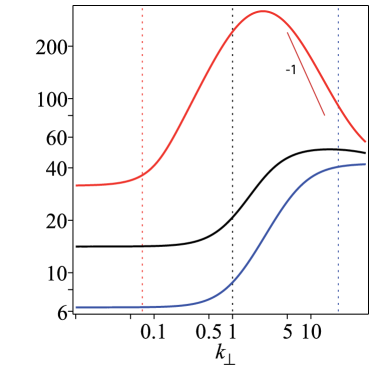
Figure 1: Phase velocity of KAWs $v_{ph}$ versus $k_{\perp}$ for $\beta_{e}=0.002$, $\tau=100$ (red), $\beta_{e}=0.01$, $\tau=0.5$ (black) and $\beta_{e}=0.05$, $\tau=0.001$ (blue). The vertical dotted lines refer to the inverse ion Larmor radius $\rho_{i}^{-1}$ for the three values of $\tau$, with the same color code as for $v_{ph}$. Transition between MHD and sub-ion scales occurs at the smallest of the two scales $\rho_{i}$ and $\rho_{s}$ (which corresponds to $k_{\perp}=1$). The orange straight line indicates the $k_{\perp}^{-1}$ asymptotic behavior in the large $\tau$ limit.

The associated eigenmodes obey

$${\widehat{A}}=\frac{\beta_{e}}{2}v_{ph}\frac{{\widehat{M}}_{2}}{k_{\perp}^{2}}{\widehat{\varphi}}.$$ (163)

A graph of $v_{ph}(k_{\perp})$ is displayed in Fig. 1 for the cases $\beta_{e}=0.002$, $\tau=100$ (red), $\beta_{e}=0.01$, $\tau=0.5$ (black) and $\beta_{e}=0.05$, $\tau=0.001$ (blue). An important difference that appears at large $\tau$, in addition to the shift of the dispersive zone towards smaller $k_{\perp}$ (due to the fact that $\rho_{i}$ is larger than $\rho_{s}$, here by a factor $\sqrt{200}$), is that at sub-$d_{e}$ scales, $v_{ph}$ does not stay constant but decreases as $k_{\perp}$ increases (asymptotically like $k_{\perp}^{-1}$ in the large $\tau$ limit), as in the full kinetic theory Passot et al. (2017). In the absence of the $\delta^{2}$ term in $L_{3}$, $v_{ph}$ would be constant at small scales.

Interestingly, when assuming relation (163) in formula (155) for the energy ${\mathcal{E}}$, the sum of the first two terms of the energy ${\mathcal{E}}$ equals that of the last three ones.

The magnetic compressibility $\chi=|{\widehat{B}}_{z}|^{2}/|\widehat{{\boldsymbol{B}}}_{\perp}|^{2}$ associated with the Alfvén eigenmode is then given by

$$\chi=\frac{2}{\beta_{e}}\left({1+\frac{2\delta^{2}k_{\perp}^{2}}{\beta_{e}}}\right)\frac{{\widehat{M}_{1}}^{2}}{(1-{\widehat{M}_{1}}+{\widehat{M}_{2}}){\widehat{M}_{2}}}.$$ (164)

Small $\tau$ limit ($\tau\sim\beta_{e}^{\frac{1}{2}}$): In this regime, ${\widehat{M}}_{1}\sim\beta_{e}k_{\perp}^{2}/2$ and is thus negligible (and so is $B_{z}$). On the other hand, ${\widehat{M}}_{2}=(1-\Gamma_{0})/\tau+O(\delta^{2})\approx k_{\perp}^{2}(1-3\tau k_{\perp}^{2}/4)$, leading to the dispersion relation

$$\left(\frac{\omega}{k_{z}}\right)^{2}=\frac{2}{\beta_{e}}\frac{1}{1+\frac{2\delta^{2}k_{\perp}^{2}}{\beta_{e}}}(1+k_{\perp}^{2}+\frac{3}{4}\tau k_{\perp}^{2}),$$ (165)

consistent with the fluid formula given by Eq. (187).

IV.2 Absolute equilibria

The invariants can be rewritten

$${\cal E} = \frac{1}{2}\int\Big{[}(1-{\widehat{M}}_{1}+{\widehat{M}}_{2}){\widehat{M}}_{2}|{\widehat{\varphi}}|^{2}$$ (166)

$$+\frac{2k_{\perp}^{2}}{\beta_{e}}\left(1+\frac{2\delta^{2}k_{\perp}^{2}}{\beta_{e}}\right)|{\widehat{A}_{\|}}|^{2}\Big{)}\Big{]}d^{2}{\boldsymbol{k}}_{\perp}dk_{z}$$

$${\cal H} = -\frac{1}{2}\int\Big{[}{\widehat{M}}_{2}\left(1+\frac{2\delta^{2}k_{\perp}^{2}}{\beta_{e}^{2}}\right)({\widehat{\varphi}}_{R}{\widehat{A}}_{\|R}+\widehat{\varphi_{I}}{\widehat{A}_{\|I}})\Big{]}$$ (167)

$$d^{2}{\boldsymbol{k}}_{\perp}dk_{z}$$

with ${\widehat{\varphi}}={\widehat{\varphi}}_{R}+i{\widehat{\varphi}}_{I}$ and $\widehat{A}_{\|}=\widehat{A}_{\|R}+i\widehat{A}_{\|I}$, when separating real and imaginary parts.

Based on the existence of such quadratic invariants, a classical tool for predicting the direction of turbulent cascades is provided by the behavior of the spectral density of the corresponding invariants in the regime of absolute equilibrium. Albeit turbulence is intrinsically a non-equilibrium regime and a turbulent spectrum strongly differs from an equilibrium spectrum, the increasing or decreasing variation of the latter in the considered spectral range can be viewed as reflecting the direction of the turbulent transfer and thus the direct or inverse character of the cascade. An early application of this approach to incompressible MHD is found in Ref. Frisch et al. (1975).

In order to apply equilibrium statistical mechanics to the system consisting in a finite number of Fourier modes obtained by spectral truncation of the fields $A_{\|}$ and $\varphi$ governed by Eqs. (141) and (144), one first easily checks that the solution satisfies the Liouville’s theorem conditions in the form

$$\sum_{\boldsymbol{k}}\frac{\partial}{\partial{\widehat{\varphi}}_{R{\boldsymbol{k}}}}\left(\frac{\partial{\widehat{\varphi}}_{R{\boldsymbol{k}}}}{\partial t}\right)+\frac{\partial}{\partial{\widehat{\varphi}}_{I{\boldsymbol{k}}}}\left(\frac{\partial{\widehat{\varphi}}_{I{\boldsymbol{k}}}}{\partial t}\right)=0$$ (168)

$$\sum_{\boldsymbol{k}}\frac{\partial}{\partial{\widehat{A}}_{\|R{\boldsymbol{k}}}}\left(\frac{\partial{\widehat{A}}_{\|R{\boldsymbol{k}}}}{\partial t}\right)+\frac{\partial}{\partial{\widehat{A}}_{\|I{\boldsymbol{k}}}}\left(\frac{\partial{\widehat{A}}_{\|{\boldsymbol{k}}}}{\partial t}\right)=0.$$ (169)

The density in phase space of the canonical equilibrium ensembles for the system (141)-(142), truncated in Fourier space, is given by $\rho=Z^{-1}\exp(-\lambda\mathcal{E}-\mu\mathcal{H})=Z^{-1}\exp(-M_{ij}x^{i}x^{j}/2)$, where $Z$ is the partition function. The matrix $M$ is defined as

$$\quad{\mathbf{M}}=\begin{bmatrix}f&0&h&0\\ 0&f&0&h\\ h&0&g&0\\ 0&h&0&g\end{bmatrix}$$

where $f=\lambda(1-{\widehat{M}}_{1}+{\widehat{M}}_{2}){\widehat{M}}_{2}$, $g=\lambda\frac{2k_{\perp}^{2}}{\beta_{e}}\left(1+\frac{2\delta^{2}k_{\perp}^{2}}{\beta_{e}}\right)$ and $h=\frac{\mu}{2}{\widehat{M}}_{2}\left(1+\frac{2\delta^{2}k_{\perp}^{2}}{\beta_{e}^{2}}\right)$. Here, $\lambda$ and $\mu$ denote numerical constants prescribed by the values of the total energy and helicity. The symbols $x^{i}_{i=1,4}$ refer to ${\widehat{\varphi}}_{R}$, ${\widehat{\varphi}}_{I}$, $\widehat{A}_{\|R}$ and $\widehat{A}_{\|I}$. The inverse matrix easily writes

$$\quad{\mathbf{M}}^{-1}=\frac{1}{\Delta}\begin{bmatrix}g&0&-h&0\\ 0&g&0&-h\\ -h&0&f&0\\ 0&-h&0&f\end{bmatrix},$$

with $\Delta=fg-h^{2}$. Without dissipation, the statistical equilibrium has an energy spectral density

$$E_{k}\sim\frac{1}{\lambda}2\pi k(fE^{\varphi}_{k}+gE_{k}^{A_{\|}})$$ (170)

and a helicity spectral density

$$H_{k}\sim\frac{1}{\mu}4\pi k_{\perp}hE_{k}^{\varphi A_{\|}},$$ (171)

where $E_{k}^{\varphi}=g/\Delta$, $E_{k}^{A_{\|}}=f/\Delta$ and $E_{k}^{\varphi A_{\|}}=-h/\Delta$.

The cascade directions are forward or backward, depending on whether the absolute equilibrium spectra are respectively growing or decreasing in the wavenumber ranges of interest. The energy spectrum rewrites

$$E_{k}\sim\frac{4\pi}{\lambda}\frac{k_{\perp}}{1-\frac{\mu^{2}}{4\lambda^{2}}\frac{1}{v_{ph}^{2}}}.$$ (172)

Positivity condition prescribes constraints on the wavenumber domain where this formula applies. The condition $\mu/\lambda\lesssim 2\min(v_{ph})$ (where $\min(v_{ph})=\sqrt{8/\beta_{e}}$ for small $\tau$ but is smaller for larger values of $\tau$), ensures that the energy spectrum is defined for all wavenumbers. For larger values of $\mu/\lambda$, there is a lower bound in $k_{\perp}$ and possibly also an upper bound, for which $E_{k}>0$. As $v_{ph}$ is bounded from above, it might happen that the energy is never positive. A more detailed study would require to explicitly relate the constants $\mu$ and $\lambda$ to the total energy and helicity. Nevertheless, in all the cases where it is defined, the energy is found to be a growing function of $k_{\perp}$ (except possibly near the lower $k_{\perp}$ bound where it has a singular behavior), whatever the values of $\beta_{e}$ and $\tau$, indicating a forward cascade. The generalized helicity spectrum, on the other hand, rewrites

$$H_{k}\sim-\frac{4\pi}{\mu}\frac{k_{\perp}}{\frac{4\lambda^{2}}{\mu^{2}}v_{ph}^{2}-1},$$ (173)

which is negative. We thus have the relation $H_{k}=-\mu/(4\lambda)E_{k}/v_{ph}^{2}$. Note however that there is no definite sign for this spectrum. In the same wavenumber ranges where the energy is positive, its absolute value is a growing quantity both at MHD and sub-$d_{e}$ scales. However, in the intermediate (sub-$\rho_{s}$ or sub-$\rho_{i}$) range, where $\omega/k_{z}\sim k_{\perp}$, it is a decreasing function of $k_{\perp}$, indicating an inverse cascade. Note that when the $-7/3$ power law of the turbulent transverse magnetic energy spectrum is not well developed (see next Section), the range of generalized helicity inverse cascade is also very limited. Similar results showing an inverse (or direct) helicity cascade in the Hall (respectively sub-electronic) range are obtained in Ref. Miloshevich et al. (2017) based on absolute equilibrium arguments in extended MHD (XMHD).

IV.3 Turbulent spectra

IV.3.1 Energy cascade

We here discuss the turbulent state in the presence of a small amount of dissipation at small scales (leading to a finite flux of energy), focusing on the case of a critically balanced KAW cascade (with equal amount of positively and negatively propagating waves). Following the discussion of Section 7 in Ref. Passot et al. (2017), the magnetic spectrum is easily obtained by imposing a constant energy flux, estimated by ratio of the spectral energy density at a given scale by the nonlinear transfer time at this scale. In the strong wave (critically-balanced) turbulence regime, this energy transfer time reduces to the nonlinear timescale. To estimate these quantities, it is first necessary to relate the Fourier components of the electric and magnetic potentials. This is achieved assuming the linear relationship provided by Eq. (163), characteristic of Alfvén modes. After inserting this relation into the energy ${\mathcal{E}}$ one finds that the total 3D spectral energy density writes

$${\mathcal{E}}^{3D}_{{\boldsymbol{k}}}=\frac{2}{\beta_{e}}k_{\perp}^{2}\left(1+\frac{2\delta^{2}k_{\perp}^{2}}{\beta_{e}}\right)|{\widehat{A}}_{\boldsymbol{k}}|^{2}$$ (174)

Due to the quasi-2D character of the dynamics, it is convenient to deal with the 2D energy spectrum

$${\mathcal{E}^{2D}_{k}}=\frac{2}{\beta_{e}}k_{\perp}^{2}\left(1+\frac{2\delta^{2}k_{\perp}^{2}}{\beta_{e}}\right)|{\widehat{A}}_{k_{\perp}}|^{2}$$ (175)

where we used the notation

$$|{\widehat{A}}_{k_{\perp}}|^{2}=\int|{\widehat{A}}_{\boldsymbol{k}}|^{2}dk_{z},$$ (176)

and assume statistical isotropy in the transverse plane. Similar definitions are used for the other relevant fields, namely the electrostatic potential $\varphi$ and the transverse magnetic field ${\boldsymbol{B}}_{\perp}$.

The nonlinear timescale is estimated from Eq. (142) which, after discarding the $B_{z}$ terms (smaller by a factor $\beta_{e}$) and the $\partial_{z}$ terms, can be rewritten

$$\partial_{t}A_{e}+[\varphi,A_{e}]-[A_{\|},M_{2}\varphi]=0.$$ (177)

Assuming locality of the nonlinear interactions in Fourier space, the typical frequencies at wavenumber $k_{\perp}$ associated with the two nonlinear terms of the above equation take the form $\tau_{NL1}^{-1}({k_{\perp}})\sim k_{\perp}^{2}|\widehat{\varphi}_{k_{\perp}}|$ and $\tau_{NL2}^{-1}({k_{\perp}})\sim k_{\perp}^{2}{\widehat{M}}_{2}|\widehat{\varphi}_{k_{\perp}}|/(1+2\delta^{2}k_{\perp}^{2}/\beta_{e})$ respectively. The global nonlinear frequency of the system can be estimated by a linear combination of these two frequencies. Taking equal weights leads to the estimate

$$\tau_{NL}^{-1}({k_{\perp}})\sim\frac{2}{\beta_{e}}k_{\perp}^{4}\left(1+\frac{\widehat{M}_{2}}{1+\frac{2\delta^{2}k_{\perp}^{2}}{\beta_{e}}}\right)\frac{1}{\widehat{M}_{2}v_{ph}}|\widehat{A}_{k_{\perp}}|.$$ (178)

In two-dimensions, when assuming isotropy, the transverse magnetic energy spectral density $|\widehat{B_{\perp}}({k_{\perp}})|^{2}\sim k_{\perp}^{2}|{\widehat{A}}_{k_{\perp}}|^{2}$ is related to the transverse magnetic energy spectrum by $E_{B_{\perp}}(k_{\perp})\sim k_{\perp}^{-1}|{\widehat{B}}_{\perp}(k_{\perp})|^{2}$, the energy flux $\varepsilon$ writes

$$\varepsilon\sim\frac{4}{\beta_{e}^{2}}\left(1+\frac{2\delta^{2}k_{\perp}^{2}}{\beta_{e}}+\widehat{M}_{2}\right)\frac{1}{\widehat{M}_{2}v_{ph}}k_{\perp}^{3}|\widehat{B}_{\perp}({k_{\perp}})|^{3},$$ (179)

and thus, assuming a constant energy flux, one gets

$$E_{B_{\perp}}(k_{\perp})\sim\varepsilon^{2/3}\beta_{e}^{4/3}k_{\perp}^{-3}\left(\frac{v_{ph}\widehat{M}_{2}}{1+\frac{2\delta^{2}k_{\perp}^{2}}{\beta_{e}}+\widehat{M}_{2}}\right)^{2/3}.$$ (180)

All the regimes of KAW energy cascade can be recovered from Eq. (180).

$\bullet$ MHD range

At scales large compared to $\rho_{s}$ and $\rho_{i}$, one has $v_{ph}\sim(2/\beta_{e})^{1/2}$, $\widehat{M}_{2}=k_{\perp}^{2}$ and $k\ll 1$. One thus immediately finds $E_{B}(k)\sim\varepsilon^{2/3}k_{\perp}^{-5/3}$.

$\bullet$ Sub-$\rho_{i}$ range

When $\sqrt{\beta_{e}/2}/\delta\geq k_{\perp}\gtrsim(2\tau)^{-1/2}$ and $\tau\geq 1$ (i.e. for scales smaller than the ion gyroradius (assumed larger than $\rho_{s}$), for which $\Gamma_{0}\approx 0$ and $\Gamma_{1}\approx 0$, and large enough for electron inertia to be negligible), one has $\widehat{M}_{2}\sim 1/\tau+\beta_{e}(1+\tau)/(2\tau)\sim{\rm constant}$ and $v_{ph}\sim k_{\perp}$, so that $E_{B}(k)\sim\varepsilon^{2/3}k_{\perp}^{-7/3}$.

$\bullet$ Sub-$\rho_{s}$ range

When, on the other hand, $\tau\leq 1$, for scales intermediate between $\rho_{s}$ and $d_{e}$, characterized by $k_{\perp}\gg 1$ and $2\delta^{2}k_{\perp}^{2}/\beta_{e}\ll 1$, one finds $\widehat{M}_{2}\sim k_{\perp}^{2}$ and $v_{ph}\sim(2/\beta_{e})^{1/2}k_{\perp}$, so that again $E_{B_{\perp}}(k_{\perp})\sim\varepsilon^{2/3}k_{\perp}^{-7/3}$. It is however to be noted that in this case, the smallest nonlinear time scale is not the stretching time $\tau_{NL1}$ but rather $\tau_{NL2}$, associated with the electron pressure term in Ohm’s law or equivalently to the Hall term, as previously mentioned.

$\bullet$ Sub-$d_{e}$ range

When $\beta_{e}$ is small enough, it is possible to observe a third power law at scales smaller that the electron inertial length (but still larger than the electron Larmor radius).

${\bf-}$ When $\tau\ll 1$, the $-7/3$ power-law zone is almost inexistent. It is replaced by a smooth transition between the $-5/3$ power-law and a steeper zone where $v_{ph}\sim{\rm cst}$, $\widehat{M}_{2}\sim k_{\perp}^{2}$ and thus where $E_{B}(k)\sim\varepsilon^{2/3}k_{\perp}^{-3}$.

${\bf-}$ If $\tau$, is taken larger than unity, $v_{ph}\sim k_{\perp}^{-1}$ and $\widehat{M}_{2}\sim k_{\perp}^{2}$, leading to $E_{B_{\perp}}(k_{\perp})\sim\varepsilon^{2/3}k_{\perp}^{-11/3}$.

${\bf-}$ Note that for a small range of parameters where $\beta_{e}\ll 1$ and $\tau=O(1)$, a regime where one can have $v_{ph}\sim{\rm constant}$ and $\widehat{M}_{2}\sim{\rm constant}$, one recovers a spectrum of the form $E_{B_{\perp}}(k_{\perp})\sim\varepsilon^{2/3}k_{\perp}^{-13/3}$, as mentioned in Ref. Passot et al. (2017).

IV.3.2 Generalized helicity cascade

We here derive the expected transverse magnetic energy spectrum associated with a generalized helicity cascade. Proceeding as in the case of the energy cascade, we first write the 3D spectral density (taken positive)

$${\cal H}^{3D}_{k}=\frac{1}{\beta_{e}v_{ph}}(1+\frac{2\delta^{2}k^{2}}{\beta_{e}})k_{\perp}^{2}|\widehat{A}_{\boldsymbol{k}}|^{2}.$$ (181)

Keeping the same estimate for the transfer time, and assuming a constant generalized helicity flux rate $\eta$, we obtain the magnetic spectrum in the helicity cascade

$$E_{B_{\perp}}(k_{\perp})\sim\eta^{2/3}\beta_{e}^{4/3}k_{\perp}^{-3}\left(\frac{v_{ph}^{2}\widehat{M}_{2}}{1+\frac{2\delta^{2}k_{\perp}^{2}}{\beta_{e}}+\widehat{M}_{2}}\right)^{2/3}.$$ (182)

Going through the same estimates in the various wavenumber domains as for the energy cascade, we now see that the magnetic spectrum in the helicity cascade obeys a $-5/3$ power law from the MHD range to the electron scale. At scales smaller that $d_{e}$, we differently finds that for $\tau\ll 1$ the spectrum is proportional to $k_{\perp}^{-3}$, while it is otherwise proportional to $k_{\perp}^{-13/3}$.

It is of interest to remark that this latter scaling is somewhat similar to the $M_{H+}$ spectrum of Abdelhamid et al. (2016) associated to the magnetic spectrum of the magneto-sonic cyclotron branch in the so-called H-generalized helicity cascade computed on exact solutions of an extended MHD model (with the caveat that in Abdelhamid et al. (2016) a singularity appears at the $d_{e}$ scale).

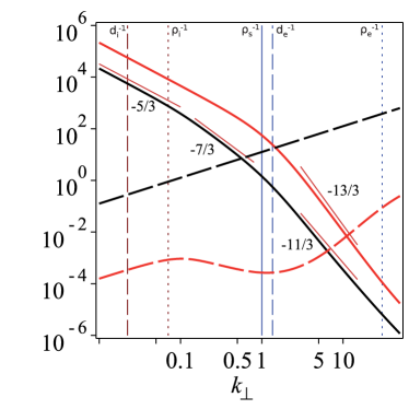
Figure 2: Turbulent magnetic spectra (solid lines) in energy (black) and generalized helicity (red) cascades, together with absolute equilibrium energy (black long dashed lines) and generalized helicity (red long dashed lines) spectra for $\beta_{e}=0.002$, $\tau=100$. Straight orange lines refer to the slopes of the various power-law inertial ranges: $-5/3$ in the MHD range, $-7/3$ in the sub-ion Larmor radius range and $-11/3$ (for the energy cascade) or $-13/3$ (for the helicity cascade) in the sub-$d_{e}$ range. The blue solid vertical line refers to $\rho_{s}^{-1}$, the brown and blue long-dashed (respectively dotted) vertical lines to the inverse ion and electron inertial lengths (respectively Larmor radii) $d_{i}^{-1}$ and $d_{e}^{-1}$ (respectively $\rho_{i}^{-1}$ and $\rho_{e}^{-1}$).

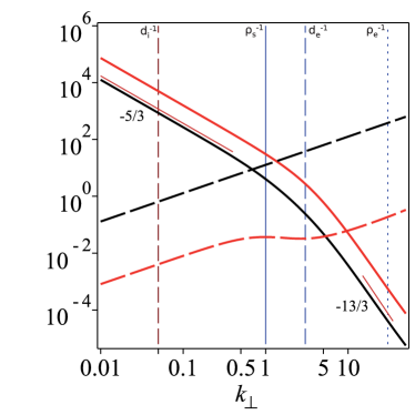
Figure 3: Same as for Fig. 2 for $\beta_{e}=0.01$, $\tau=0.5$. No sub-ion power-law range is visible. Both for the energy and helicity cascades, the magnetic spectrum displays a $-13/3$ sub-$d_{e}$ power-law range.

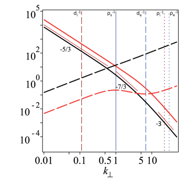
Figure 4: Same as for Fig. 2 for $\beta_{e}=0.05$, $\tau=0.001$. A $-7/3$ power-law turbulent magnetic spectrum in the energy cascade is visible for $k_{\perp}>1$, while, both for the energy and helicity cascades, the magnetic spectrum displays a $-3$ sub-$d_{e}$ power-law range.

Examples of transverse magnetic energy spectra are displayed for the parameters $\beta_{e}=0.002$, $\tau=100$ (Fig. 2), $\beta_{e}=0.01$, $\tau=0.5$ (Fig. 3) and $\beta_{e}=0.05$, $\tau=0.001$ (Fig. 4), both for the absolute equilibria (long dashed lines) of the energy (black) and the generalized helicity (red) and for the turbulent magnetic spectra (solid lines) associated to the energy cascade (black) and the helicity cascade (red). The helicity inverse cascade associated with the decreasing absolute equilibrium spectrum in sub-ion range, is conspicuous in the case of large $\tau$, but less pronounced for $\tau$ of order unity.

V Discussion and conclusion

In this paper, two new reduced models have been derived for low-$\beta_{e}$ plasmas. One of them, given by Eqs. (55)-(60), concerns the small $\tau$-regime and extends the four-field model of Ref. Hsu et al. (1986) by retaining electron inertia. Both a fluid derivation and a reduction of the gyrofluid model of Ref. Brizard (1992) are presented. Interestingly, agreement between the two formulations requires closure assumptions consistent with the underlying scaling, such as adiabatic ions. The other model, given by Eqs. (148)-(149), is a two-field gyrofluid model, valid for any $\tau$, which retains both electron inertia and $B_{z}$ fluctuations, in addition to ion FLR contributions. It is used to present a comprehensive phenomenological description of the Alfvén wave magnetic energy spectrum from the MHD scales to scales smaller than $d_{e}$ (while larger than $\rho_{e}$). Assuming the existence of energy or helicity cascades, this leads to the prediction of the magnetic energy spectrum when neglecting possible intermittency effects originating from the presence of coherent structures. The existence of these cascades needs to be confirmed by numerical simulations of the gyrofluid equations supplemented by dissipation and energy and/or helicity injection. In particular, the inverse helicity cascade is expected to occur only when the system is driven at a scale close to $d_{e}$, in a way that mostly injects helicity rather than energy. In fact, Eq. (161) shows that a non-zero helicity corresponds to an imbalanced regime where either $G_{+}$ or $G_{-}$ dominates. It is interesting to note that the evidence of an inverse helicity cascade in numerical simulations of imbalanced EMHD turbulence was reported in Refs. Cho (2016); Kim and Cho (2015). Analytic considerations on the role of helicity in weak REMHD turbulence can also be found in Ref. Galtier and Meyrand (2015). An imbalanced energy injection could possibly originate from magnetic reconnection that takes place at the electronic scales. This scenario was recently considered in Ref. Franci et al. (2017) on the basis of 2D hybrid PIC and Vlasov simulations where the development of a sub-ion magnetic energy spectrum occurs in relation with the reconnection instability, before the direct energy cascade reaches this scale.

In the framework of the two-field gyrofluid model, the transition scale between the $k_{\perp}^{-5/3}$ and the $k_{\perp}^{-7/3}$ ranges occurs at the largest of the two scales $\rho_{i}$ and $\rho_{s}$. When $\tau$ is small, this will also be the case with Eqs. (55)-(60) that retain the coupling to $n=-(2/\beta_{e})B_{z}$ and $u_{i}$, as shown by using the same arguments as in Appendix E.4 of Ref. Schekochihin et al. (2009). Differently for $\tau\sim 1$ and small $\beta_{e}$, a spectral transition is observed to take place at scale $d_{i}$, both in the solar wind Chen et al. (2014) and in hybrid-PIC simulations Franci et al. (2016). The question arises whether a similar transition could also be observed in numerical simulations of reduced models, induced by the presence of current sheets and the occurence of reconnection processes, or if more physics has to be taken into account.

Note that while the magnetic energy spectrum displays a $k_{\perp}^{-7/3}$ range both below the ion Larmor radius and below $\rho_{s}$ when $\beta_{e}$ is small, the perpendicular electric field spectrum scales like $k_{\perp}^{-1/3}$ in the former regime and like $k_{\perp}^{-13/3}$ in the latter one.

The two-field gyrofluid model derived in this paper could be extended to account for electron Landau damping, a crucial ingredient at small $\beta_{e}$, with either a Landau fluid formulation, as suggested in Ref. Passot et al. (2017), or with the coupling with a drift-kinetic equation. In the latter case, it could provide an interesting generalization of the model presented in Zocco and Schekochihin (2011), by taking into account the parallel magnetic field fluctuations and thus permitting larger values of $\beta_{e}$.

At sub-$d_{e}$ scales, a new regime is uncovered in the case of cold ions (small $\tau$), where the magnetic energy density scales like $k_{\perp}^{-3}$. Compressibility here plays a central role, which explains the difference with the cases $\tau\sim 1$ where the spectrum scales like $k_{\perp}^{-13/3}$ or $\tau\gg 1$ (a quasi-incompressible limit) where it scales like $k_{\perp}^{-11/3}$. Scales smaller than $\rho_{e}$ are not considered in this paper, as they require a full description of the electron FLR effects. In this regime, the spectrum is observed to be even steeper Huang et al. (2014), possibly associated with a phase-space entropy cascade Schekochihin et al. (2009).

We have here considered the regime of strong wave turbulence where critical balance holds. Due to this property, the estimates of the nonlinear times and the relation between the fields turn out to be identical to those of the purely non-linear regime that occurs for example in two dimensions.

Acknowledgments: We are thankful to W. Dorland for useful discussions.

Appendix A Dispersion relation

The system (55)-(58), when linearized about a uniform state, leads to

$$\frac{\omega}{k_{z}}(1+\frac{5\tau}{4}k_{\perp}^{2})\widehat{\varphi^{*}}-\frac{2}{\beta_{e}}(1+\frac{\tau}{2}k_{\perp}^{2})\widehat{A_{\|}}=0$$ (183)

$$-\frac{\omega}{k_{z}}((1+\delta^{2}+\tau k_{\perp}^{2})\widehat{u_{i}}-\frac{2\delta^{2}}{\beta_{e}}k_{\perp}^{2}\widehat{A_{\|}})$$

$$+(1+\tau)\widehat{n}+\tau k_{\perp}^{2}\widehat{\varphi^{*}}=0$$ (184)

$$-\frac{\omega}{k_{z}}\widehat{n}+\widehat{u_{i}}-\frac{2}{\beta_{e}}k_{\perp}^{2}\widehat{A_{\|}}=0$$ (185)

$$-\frac{\omega}{k_{z}}((1+\frac{2\delta^{2}}{\beta_{e}}k_{\perp}^{2})\widehat{A_{\|}}-\delta^{2}\widehat{u_{i}})+(1+\frac{\tau}{2}k_{\perp}^{2})\widehat{\varphi^{*}}$$

$$-(1+\tau)\widehat{n}=0,$$ (186)

where $\omega$, $k_{z}$, $k_{\perp}$ are respectively the frequency, parallel and perpendicular wavenumbers of harmonic perturbations whose Fourier complex coefficients are denoted with a $\widehat{.}$ symbol. This system supports two kind of waves, kinetic Alfvén waves (KAWs) and slow-magnetosonic waves (SWs). Ion parallel velocity plays a minor role in the dispersion relation of KAWs that can thus be approximated by

$$(\frac{\omega}{k_{z}})^{2}=\frac{2}{\beta_{e}}\frac{1}{1+\frac{2\delta^{2}k_{\perp}^{2}}{\beta_{e}}}\left((1+\tau)k_{\perp}^{2}+\frac{(1+\tau k_{\perp}^{2}/2)^{2}}{1+5\tau k_{\perp}^{2}/4}\right).$$ (187)

It turns out that this approximation is excellent for a wide range of values of $\tau$ and $\beta_{e}$ in the whole spectral domain. Another simplification consisting in taking the cold ion limit and dropping some subdominant contributions proportional to $\delta^{2}$, allows one to obtain the slow branch. The dispersion relation then reduces to

$$\Big{(}(\frac{\omega}{k_{z}})^{2}-1\Big{)}\Big{(}(\frac{\omega}{k_{z}})^{2}-\frac{2}{\beta_{e}}\Big{)}+\frac{2k_{\perp}^{2}}{\beta_{e}}(\frac{\omega}{k_{z}})^{2}\Big{(}\delta^{2}(\frac{\omega}{k_{z}})^{2}-1\Big{)}=0.$$ (188)

It is easy to verify that the KAW dispersion relation given in Eq. (187) taken for $\tau=0$, can be recovered from Eq. (188) when $\frac{\omega}{k_{z}}\gg 1$. The slow magnetosonic branch is such that $\frac{\omega}{k_{z}}\sim 1$ at large scale, with a small dispersive component at small scale (a good approximation to the solution is given by $\omega/k_{z}=(1+k_{\perp}^{2})^{-1/2}$). From these results, one can estimate, for both kinds of waves and within scaling II, the values of $\zeta_{r}=\omega/(k_{z}v_{thr})$ both for ions (for which $v_{thi}\sim\tau^{1/2}\sim\delta^{1/2}$) and for electrons (for which $v_{the}\sim\delta^{-1}$). On has, for KAWs, $\zeta_{i}\sim\delta^{-3/2}\gg 1$ and $\zeta_{e}\sim 1$, while for SWs, $\zeta_{i}\sim\delta^{-1/2}\gg 1$ and $\zeta_{e}\sim\delta\ll 1$. It is thus a reasonable approximation to assume adiabatic ions and isothermal electrons. The good agreement between kinetic theory and an isothermal equation of state for the electrons, even when $\zeta_{e}\sim 1$, is shown in Ref. Passot et al. (2017).

Appendix B Parent gyrofluid model

We adopt the same definitions of Ref. Tassi et al. (2016) and consider the following gyrofluid equations for the evolutions of the gyrocenter moments $N_{e,i}$, $U_{e,i}$, $P_{\parallel e,i}$, $P_{\perp e,i}$, $Q_{\parallel e,i}$, $Q_{\perp e,i}$, $R_{\parallel\perp e,i}$ and $R_{\perp\perp e,i}$ corresponding to the the normalized fluctuations of gyrocenter density, parallel velocity, parallel and perpendicular pressure, parallel and perpendicular heat flux, and of the parallel/parallel and parallel/perpendicular components of the energy weighted pressure tensor respectively, with the subscript $e$ and $i$ referring to electrons and ions

$$\frac{\partial N_{e}}{\partial t}+[\mathrm{e}^{\delta^{2}\Delta_{s}}\varphi,N_{e}]+\delta^{2}[\Delta_{s}\mathrm{e}^{\delta^{2}\Delta_{s}}\varphi,P_{\perp e}-N_{e}]-[\mathrm{e}^{\delta^{2}\Delta_{s}}A_{\parallel},U_{e}]$$

$$-[\mathrm{e}^{\delta^{2}\Delta_{s}}B_{z},P_{\perp e}]-\delta^{2}[\Delta_{s}\mathrm{e}^{\delta^{2}\Delta_{s}}B_{z},P_{\perp e}-N_{e}]+\frac{\partial U_{e}}{\partial z}=0,$$ (189)

$$\frac{\partial}{\partial t}\left(\delta^{2}U_{e}-\mathrm{e}^{\delta^{2}\Delta_{s}}A_{\parallel}\right)+\delta^{2}[\mathrm{e}^{\delta^{2}\Delta_{s}}\varphi,U_{e}]-[\mathrm{e}^{\delta^{2}\Delta_{s}}A_{\parallel},P_{\parallel e}]$$

$$-\delta^{2}[\Delta_{s}\mathrm{e}^{\delta^{2}\Delta_{s}}A_{\parallel},P_{\perp e}-N_{e}]-\delta^{2}[\mathrm{e}^{\delta^{2}\Delta_{s}}B_{z},U_{e}]-\delta^{2}[B_{z},Q_{\perp e}]$$

$$-{\overline{\Gamma}}_{0}(\delta^{2}\Delta_{s}^{\varphi},\delta^{2}\Delta_{s}^{A})[\varphi,A_{\parallel}]$$

$$+({\overline{\Gamma}}_{0}(\delta^{2}\Delta_{s}^{B},\delta^{2}\Delta_{s}^{A})+\delta^{2}\Delta_{s}{\overline{\Gamma}}_{1}(\delta^{2}\Delta_{s}^{B},\delta^{2}\Delta_{s}^{A}))[B_{z},A_{\parallel}]$$

$$+\frac{\partial}{\partial z}\left(P_{\parallel e}-\mathrm{e}^{\delta^{2}\Delta_{s}}\varphi+\mathrm{e}^{\delta^{2}\Delta_{s}}B_{z}\right)=0,$$ (190)

$$\frac{\partial P_{\parallel e}}{\partial t}+[\mathrm{e}^{\delta^{2}\Delta_{s}}\varphi,P_{\parallel e}]+\delta^{2}[\Delta_{s}\mathrm{e}^{\delta^{2}\Delta_{s}}\varphi,P_{\perp e}-N_{e}]-2[A_{\parallel},Q_{\parallel e}]$$

$$-3[\mathrm{e}^{\delta^{2}\Delta_{s}}A_{\parallel},U_{e}]-[\mathrm{e}^{\delta^{2}\Delta_{s}}B_{z},P_{\parallel e}+P_{\perp e}-N_{e}]$$

$$-\delta^{2}[\Delta_{s}\mathrm{e}^{\delta^{2}\Delta_{s}}B_{z},P_{\perp e}-N_{e}]-[B_{z},R_{\|\perp e}]$$

$$+\frac{\partial}{\partial z}\left(Q_{\parallel e}+3U_{e}\right)=0,$$ (191)

$$\frac{\partial P_{\perp e}}{\partial t}+[(1+\delta^{2}\Delta_{s})\mathrm{e}^{\delta^{2}\Delta_{s}}\varphi,P_{\perp e}]$$

$$+\delta^{2}[\Delta_{s}(2+\delta^{2}\Delta_{s})\mathrm{e}^{\delta^{2}\Delta_{s}}\varphi,P_{\perp e}-N_{e}]-[\mathrm{e}^{\delta^{2}\Delta_{s}}A_{\parallel},U_{e}]$$

$$-[A_{\parallel},Q_{\perp e}]-[(2+\delta^{2}\Delta_{s})\mathrm{e}^{\delta^{2}\Delta_{s}}B_{z},2P_{\perp e}-N_{e}]$$

$$-\delta^{2}[\Delta_{s}(3+\delta^{2}\Delta_{s})\mathrm{e}^{\delta^{2}\Delta_{s}}B_{z},P_{\perp e}-N_{e}]$$

$$-2[B_{z},R_{\perp\perp e}]+\frac{\partial}{\partial z}\left(U_{e}+Q_{\perp e}\right)=0,$$ (192)

$$\frac{\partial N_{i}}{\partial t}+[\mathrm{e}^{\tau\Delta_{s}}\varphi,N_{i}]+\tau[\Delta_{s}\mathrm{e}^{\tau\Delta_{s}}\varphi,P_{\perp i}-N_{i}]-[\mathrm{e}^{\tau\Delta_{s}}A_{\parallel},U_{i}]$$

$$+\tau[\mathrm{e}^{\tau\Delta_{s}}B_{z},P_{\perp i}]+\tau^{2}[\Delta_{s}\mathrm{e}^{\tau\Delta_{s}}B_{z},P_{\perp i}-N_{i}]+\frac{\partial U_{i}}{\partial z}=0,$$ (193)

$$\frac{\partial}{\partial t}\left(U_{i}+\mathrm{e}^{\tau\Delta_{s}}A_{\parallel}\right)+[\mathrm{e}^{\tau\Delta_{s}}\varphi,U_{i}]-\tau[\mathrm{e}^{\tau\Delta_{s}}A_{\parallel},P_{\parallel i}]$$

$$-\tau^{2}[\Delta_{s}\mathrm{e}^{\tau\Delta_{s}}A_{\parallel},P_{\perp i}-N_{i}]+\tau[\mathrm{e}^{\tau\Delta_{s}}B_{z},U_{i}]+\tau[B_{z},Q_{\perp i}]$$

$$+{\overline{\Gamma}}_{0}(\tau\Delta_{s}^{\varphi},\tau\Delta_{s}^{A})[\varphi,A_{\parallel}]$$

$$+\tau({\overline{\Gamma}}_{0}(\tau\Delta_{s}^{B},\tau\Delta_{s}^{A})+\tau\Delta_{s}{\overline{\Gamma}}_{1}(\tau\Delta_{s}^{B},\tau\Delta_{s}^{A}))[B_{z},A_{\parallel}]$$

$$+\frac{\partial}{\partial z}\left(\tau P_{\parallel i}+\mathrm{e}^{\tau\Delta_{s}}\varphi+\tau\mathrm{e}^{\tau\Delta_{s}}B_{z}\right)=0,$$ (194)

$$\frac{\partial P_{\parallel i}}{\partial t}+[\mathrm{e}^{\tau\Delta_{s}}\varphi,P_{\parallel i}]+\tau[\Delta_{s}\mathrm{e}^{\tau\Delta_{s}}\varphi,P_{\perp i}-N_{i}]-2[A_{\parallel},Q_{\parallel i}]$$

$$-3[\mathrm{e}^{\tau\Delta_{s}}A_{\parallel},U_{i}]+\tau[\mathrm{e}^{\tau\Delta_{s}}B_{z},P_{\parallel i}+P_{\perp i}-N_{i}]$$

$$+\tau^{2}[\Delta_{s}\mathrm{e}^{\tau\Delta_{s}}B_{z},P_{\perp i}-N_{i}]+\tau[B_{z},R_{\|\perp i}]$$

$$+\frac{\partial}{\partial z}\left(Q_{\parallel i}+3U_{i}\right)=0,$$ (195)

$$\frac{\partial P_{\perp i}}{\partial t}+[(1+\tau\Delta_{s})\mathrm{e}^{\tau\Delta_{s}}\varphi,P_{\perp i}]$$

$$+\tau[\Delta_{s}(2+\tau\Delta_{s})\mathrm{e}^{\tau\Delta_{s}}\varphi,P_{\perp i}-N_{i}]$$

$$-[\mathrm{e}^{\tau\Delta_{s}}A_{\parallel},U_{i}]-[A_{\parallel},Q_{\perp i}]$$

$$+\tau[(2+\tau\Delta_{s})\mathrm{e}^{\tau\Delta_{s}}B_{z},2P_{\perp i}-N_{i}]$$

$$+\tau^{2}[\Delta_{s}(3+\tau\Delta_{s})\mathrm{e}^{\tau\Delta_{s}}B_{z},P_{\perp i}-N_{i}]$$

$$+2\tau[B_{z},R_{\perp\perp i}]+\frac{\partial}{\partial z}\left(U_{i}+Q_{\perp i}\right)=0,$$ (196)

together with Poisson’s equations and parallel and perpendicular Ampère’s laws, which respectively read

$$\frac{v_{A}^{2}}{c^{2}}\Delta_{\perp}\varphi=\mathrm{e}^{\delta^{2}\Delta_{s}}N_{e}+\delta^{2}\Delta_{s}\mathrm{e}^{\delta^{2}\Delta_{s}}(P_{\perp e}-N_{e})$$

$$-(I_{0}(2\delta^{2}\Delta_{s})\mathrm{e}^{2\delta^{2}\Delta_{s}}-1)\varphi$$

$$+(I_{0}(2\delta^{2}\Delta_{s})-I_{1}(2\delta^{2}\Delta_{s}))\mathrm{e}^{2\delta^{2}\Delta_{s}}B_{z}$$

$$-\mathrm{e}^{\tau\Delta_{s}}N_{i}-\tau\Delta_{s}\mathrm{e}^{\tau\Delta_{s}}(P_{\perp i}-N_{i})-(I_{0}(2\tau\Delta_{s})\mathrm{e}^{2\tau\Delta_{s}}-1)\frac{\varphi}{\tau}$$

$$-(I_{0}(2\tau\Delta_{s})-I_{1}(2\tau\Delta_{s}))\mathrm{e}^{2\tau\Delta_{s}}B_{z},$$ (197)

$$\begin{split}\Delta_{\perp}A_{\parallel}=\frac{\beta_{e}}{2}(\mathrm{e}^{\delta^{2}\Delta_{s}}U_{e}-\mathrm{e}^{\tau\Delta_{s}}U_{i}),\end{split}$$ (198)

and

$$\begin{split}&B_{z}=-\frac{\beta_{e}}{2}\left(\mathrm{e}^{\delta^{2}\Delta_{s}}P_{\perp e}+\delta^{2}\Delta_{s}\mathrm{e}^{\delta^{2}\Delta_{s}}(P_{\perp e}-N_{e})\right.\\ &\left.-(I_{0}(2\delta^{2}\Delta_{s})-I_{1}(2\delta^{2}\Delta_{s}))\mathrm{e}^{2\delta^{2}\Delta_{s}}\varphi\right.\\ &\left.+2(I_{0}(2\delta^{2}\Delta_{s})-I_{1}(2\delta^{2}\Delta_{s}))\mathrm{e}^{2\delta^{2}\Delta_{s}}B_{z}\right.\\ &\left.+\tau\mathrm{e}^{\tau\Delta_{s}}P_{\perp i}+\tau^{2}\Delta_{s}\mathrm{e}^{\tau\Delta_{s}}(P_{\perp i}-N_{i})\right.\\ &\left.+(I_{0}(2\tau\Delta_{s})-I_{1}(2\tau\Delta_{s}))\mathrm{e}^{2\tau\Delta_{s}}\varphi\right.\\ &\left.+2\tau(I_{0}(2\tau\Delta_{s})-I_{1}(2\tau\Delta_{s}))\mathrm{e}^{2\tau\Delta_{s}}B_{z}\right).\end{split}$$ (199)

The operators ${\overline{\Gamma}}_{0}$ and ${\overline{\Gamma}}_{1}$ and $\Delta_{s}$ are defined as ${\overline{\Gamma}}_{0}(z,z^{\prime})=I_{0}(zz^{\prime})\exp(z+z^{\prime})$, ${\overline{\Gamma}}_{1}(z,z^{\prime})=I_{1}(zz^{\prime})\exp(z+z^{\prime})$ and $\Delta_{s}=\frac{1}{2}\Delta_{\perp}$, with $I_{0}$ and $I_{1}$ indicating the modified Bessel function of the first kind of order zero and one, respectively.

The set of gyrofluid equations (189)-(199) was derived in Ref. Brizard (1992), although with a different normalization and with the combination $I_{0}+I_{1}$ instead of $I_{0}-I_{1}$ in Eqs. (197) and (199). In Eqs. (189)-(199), we corrected a few typographical errors that were present in the corresponding equations of Ref. Tassi et al. (2016) (where they had no effect in the considered asymptotics).

References

- Passot et al. (2017) T. Passot, P. L. Sulem, and E. Tassi, J. Plasma Phys. 83, 715830402 (2017).
- Fitzpatrick and Porcelli (2004) R. Fitzpatrick and F. Porcelli, Phys. Plasmas 11, 4713 (2004).
- Fitzpatrick and Porcelli (2007) R. Fitzpatrick and F. Porcelli, Phys. Plasmas 14, 049902 (2007).
- Tassi et al. (2010) E. Tassi, P. J. Morrison, D. Grasso, and F. Pegoraro, Nucl. Fusion 50, 034007 (2010).
- Hsu et al. (1986) C. T. Hsu, R. D. Hazeltine, and P. J. Morrison, Phys. Fluids 29, 1480 (1986).
- Brizard (1992) A. Brizard, Phys. Fluids B 4, 1213 (1992).
- Cerri and Califano (2017) S. S. Cerri and F. Califano, New J. Phys. 19, 025007 (2017).
- Franci et al. (2016) L. Franci, S. Landi, L. Matteini, A. Verdini, and P. Hellinger, Astrophys. J. 833, 91 (2016), arXiv:1610.05158 [physics.space-ph] .
- Tassi et al. (2016) E. Tassi, P. L. Sulem, and T. Passot, J. Plasma Phys. 82, 705820601 (2016).
- Comisso et al. (2012) L. Comisso, D. Grasso, E. Tassi, and F. L. Waelbroeck, Physics of Plasmas 19, 042103 (2012).
- Schekochihin et al. (2009) A. A. Schekochihin, S. C. Cowley, W. Dorland, G. W. Hammett, G. G. Howes, E. Quataert, and T. Tatsuno, Astrophys. J. Suppl. 182, 310 (2009).
- Boldyrev et al. (2015) S. Boldyrev, C. H. K. Chen, Q. Xia, and V. Zhdankin, Astrophys. J. 806, 238 (2015), arXiv:1507.00416 [physics.space-ph] .
- Andrés et al. (2014) N. Andrés, L. Martin, P. Dmitruk, and D. Gómez, Phys. Plasmas 21, 072904 (2014).
- Schekochihin et al. (2010) A. A. Schekochihin, S. C. Cowley, F. Rincon, and M. S. Rosin, Mon. Not. R. Astron. Soc. 405, 291 (2010).
- Scott (2007) B. D. Scott, Phys. Plasmas 14, 102318 (2007).
- Belova (2001) E. V. Belova, Phys. Plasmas 8, 3936 (2001).
- Scott (2010) B. Scott, Phys. Plasmas 17, 102306 (2010).
- Snyder and Hammett (2001) P. B. Snyder and G. W. Hammett, Phys. Plasmas 8, 3199 (2001).
- Tassi (2015) E. Tassi, Annals of Physics 362, 239 (2015).
- Passot and Sulem (2007) T. Passot and P. L. Sulem, Phys. Plasmas 14, 082502 (2007).
- Schep et al. (1994) T. J. Schep, F. Pegoraro, and B. N. Kuvshinov, Phys. Plasmas , 2843 (1994).
- Borgogno et al. (2005) D. Borgogno, D. Grasso, F. Porcelli, F. Califano, and D. Pegoraro, F. Farina, Phys. Plasmas 12, 032309 (2005).
- Biskamp et al. (1997) D. Biskamp, E. Schwarz, and J. F. Drake, Phys. Plasmas 4, 1002 (1997).
- Chen and Boldyrev (2017) C. H. K. Chen and S. Boldyrev, Astrophys. J 842, 122 (2017), arXiv:1705.08558v1 [physics-space-ph].
- Tassi (2017) E. Tassi, Eur. Phys. J. D 71, 269 (2017).
- Morrison (1998) P. J. Morrison, Rev. Mod. Phys. 70, 467 (1998).
- Waelbroeck et al. (2009) F. L. Waelbroeck, R. D. Hazeltine, and P. J. Morrison, Phys. Plasmas 16, 032109 (2009).
- Cafaro et al. (1998) E. Cafaro, D. Grasso, F. Pegoraro, F. Porcelli, and A. Saluzzi, Phys. Rev. Lett. 80, 4430 (1998).
- Frisch et al. (1975) U. Frisch, A. Pouquet, J. Léorat, and A. Mazure, J. Fluid Mech. 68, 769 (1975).
- Miloshevich et al. (2017) G. Miloshevich, M. Lingam, and P. J. Morrison, New Journal of Physics 19, 015007 (2017).
- Abdelhamid et al. (2016) H. M. Abdelhamid, M. Lingam, and S. M. Mahajan, Astrophys. J. 829, 87 (2016).
- Cho (2016) J. Cho, J. Phys. Conf. Ser. 719, 012001 (2016).
- Kim and Cho (2015) H. Kim and J. Cho, Astrophys. J. 801, 75 (2015).
- Galtier and Meyrand (2015) S. Galtier and R. Meyrand, J. Plasma Phys. 81, 325810106 (2015).
- Franci et al. (2017) L. Franci, S. S. Cerri, F. Califano, S. Landi, E. Papini, A. Verdini, L. Matteini, F. Jenko, and P. Hellinger, Astrophys. J. Lett. 850, L16 (2017), arXiv:1707.06548 [physics.space-ph] .
- Chen et al. (2014) C. H. K. Chen, L. Leung, S. Boldyrev, B. A. Maruca, and S. D. Bale, Geophys. Res. Lett. 41, 8081 (2014).
- Zocco and Schekochihin (2011) A. Zocco and A. Schekochihin, Phys. Plasmas 18, 102309 (2011).
- Huang et al. (2014) S. Y. Huang, F. Sahraoui, X. H. Deng, J. S. He, Z. G. Yuan, M. Zhou, Y. Pang, and H. S. Fu, Astrophys. J. Lett. 789, L28 (2014).