Anomalous Exponents in Strong Turbulence

Abstract

To characterize fluctuations in a turbulent flow, one usually studies different moments of velocity increments and dissipation rate, $\overline{(v(x+r)-v(x))^{n}}\propto r^{\zeta_{n}}$ and $\overline{{\cal E}^{n}}\propto Re^{d_{n}}$, respectively. In high Reynolds number flows, the moments of different orders cannot be simply related to each other which is the signature of anomalous scaling, one of the most puzzling features of turbulent flows. High-order moments are related to extreme, rare events and our ability to quantitatively describe them is crucially important for meteorology, heat, mass transfer and other applications. In this work we present a solution to this problem in the particular case of the Navier-Stokes equations driven by a random force. A novel aspect of this work is that, unlike previous efforts which aimed at seeking solutions around the infinite Reynolds number limit, we concentrate on the vicinity of transitional Reynolds numbers $Re^{tr}$ where the first emergence of anomalous scaling is observed out of a low-$Re$ Gaussian background. The obtained closed expressions for anomalous scaling exponents $\zeta_{n}$ and $d_{n}$, which depend on the transition Reynolds number, agree well with experimental and numerical data in the literature and, when $n\gg 1$, $d_{n}\approx 0.19n\ln(n)$. The theory yields the energy spectrum $E(k)\propto k^{-\zeta_{2}-1}$ with $\zeta_{2}\approx 0.699$, different from the outcome of Kolmogorov’s theory. It is also argued that fluctuations of dissipation rate and those of the transition point itself are responsible for both, deviation from Gaussian statistics and multiscaling of velocity field.

PACS numbers 47.27

I. Introduction.
Thanks to rapid development of experimental and computational methods, Kolmogorov’s dimensional considerations of 1941, leading to the energy spectrum $E(k)\approx{\overline{\cal E}^{\frac{2}{3}}k^{2}\overline{|v(k)|^{2}}}\propto k^{-\frac{5}{3}}$, have been reasonably well supported by both physical and numerical experiments. Still, one cannot rule out some slight correction to the $5/3$ exponent. In this formula, the dissipation rate ${\cal E}=2\nu S_{pq}S_{qp}$ with $S_{pq}=(\partial_{p}v_{q}+\partial_{q}v_{p})/2$, is a fluctuating small-scale parameter and appearance of $\overline{{\cal E}}$ in Kolmogorov’s energy spectrum can be traced to Kolmogorov’s relation $\overline{(v(x+r)-v(x))^{3}}=-\frac{4}{5}\overline{{\cal E}}r$, where $v$ is the $x$-component of velocity field and $r$ is the displacement in the $x$-direction chosen in the inertial range (IR) $\eta\ll r\ll L$. Here $\eta$ and $L$ denote viscous and integral length-scales ($L)$, respectively. The energy balance in the Navier-Stokes equations gives $\overline{{\cal E}}={\cal P}$ where ${\cal P}=const$ denotes the power of external large-scale energy source. Based on a bold assumption of both ultra-violet ($\eta)$ and infra-red ($L$) cut-offs disappearance in the IR dynamics and on his own analysis of available experimental data, Kolmogorov came up with his famous expression for the energy spectrum. It is clear that, in principle, this assumption may not be correct and fluctuations of dissipation rate can somewhat modify the $5/3$ exponent and, moreover, lead to dramatic effects in all multi-point and high-order correlation functions. Kolmogorov’s theory (K41) was subsequently generalized with various “cascade models” leading to $S_{n}=\overline{(\delta_{r}v)^{n}}\equiv\overline{(v(x+r)-v(x))^{n}}\propto r^{\zeta_{n}}$ with $\zeta_{n}=n/3$. Later, it became clear that the exponents $\zeta_{n}=n/3$, contradicted experimental data pointing to the existence of much more complex relations between $\zeta_{n}$ and $\zeta_{m}$ with $m\neq n$.

In this paper we address the problem of the scaling exponents in a simplified setup of an infinite fluid driven by a Gaussian white-in-time random force acting in the range of scales $r\approx L=O(1)$. When the amplitude of the stirring force is very small, the flow is governed by linear contributions to the Navier-Stokes equations and the resulting random velocity field is Gaussian. With an increase in the forcing amplitude, at some Reynolds number ($Re^{tr}$), which we loosely call “transitional” (see below), the nonlinear and linear terms become comparable and, eventually, non-linearity dominates and deviations from Gaussianity take over. This behavior has been demonstrated in Refs. [1,2] and the transition itself was discussed in terms of breakdown of Random Phase Approximation (RPA) in Ref. [3].

In 1965, in his classic textbook [4], R.P. Feynman proclaimed turbulence “a central problem, put aside by physicists more than a century (nineteenth!) ago”, which one day we will “have to solve and we do not know how.” His point was that by 1965 we knew more about weak and strong interactions of elementary particles than about flow of water out of faucets in our bathtubs. Feynman did not elaborate on his statement and we can only guess that he had in mind a derivation of chaotic, high-Reynolds number solutions directly from deterministic and well-known Navier-Stokes equations for incompressible fluids. It also became clear (for a comprehensive review see Refs. [5]) that, due to the lack of a small coupling constant, the problem of derivation of the energy spectra and other correlation functions from the NS equations using renormalized perturbation expansions was as hard as that in the theory of strong interactions for which important advances had been achieved [6]. Today, in the 21th century, the problem is still open.

In this paper we develop a theory leading to an analytic evaluation of scaling exponents of moments of velocity derivatives including those of dissipation rate and the exponents $\zeta_{n}$ of the structure functions $S_{n}(r)=(\overline{(v(x+r)-v(x))^{n}}\propto r^{\zeta_{n}}$. An implication of the theory is that anomalous scaling is a consequence of dynamic constraints on high-order moments of velocity derivatives, following directly from the behavior of Navier-Stokes solutions at low Reynolds numbers.

This paper is organized as follows: in Section II we introduce an infinite number of $n$-dependent Reynolds numbers reflecting the multitude of anomalous exponents characterizing moments of different order $n$. In Section III, the Navier-Stokes equations driven by a random Gaussian force are introduced as a basic model treated in the paper. It is shown there that in the low-Reynolds number limit $Re\ll Re^{tr}$ the solution is Gaussian while as $Re\gg Re^{tr}$, the moments of velocity derivative are given by scaling functions with unknown anomalous exponents and amplitudes. The crossing of these two limiting curves at $Re=Re^{tr}$ gives an equations for the unknown anomalous exponents. In Section IV a transitional Reynolds numbers $R^{tr}_{\lambda,n,}$ from weakly turbulent low-Reynolds number Gaussian fluid to the high-$Re$ anomalous state is discussed. In Section V the exponents are calculated from the derived equations and compared with experimental and numerical data. Section VI is devoted to summary and discussion.

II. Local Reynolds numbers and transitions. Definitions. We are interested in an infinite fluid stirred by a Gaussian random force acting on a scale $r\approx L$. Thus, even in the limit of very weak forcing (for quantitative definitions see below) the generated flow is random. To characterize this class of flows one typically uses a Reynolds number $Re=(\delta_{r}v)_{rms}L/\nu\approx v_{rms}L/\nu$. In the “weak turbulence range”, when the forcing amplitude tends to zero and $Re\ll Re^{tr}$, the PDF of the generated velocity field is close to Gaussian. With increase of the Reynolds number to $Re\approx Re^{tr}$, the flow undergoes a transformation manifested by appearance of a broad, non-Gaussian, tails of the probability density [1-2], sometimes associated with breakdown of the Random Phase Approximation (RPA) and a phase organization discussed in [3]. Since the background flow is random, it is clear that even at $Re<Re^{tr}$, there exist low-probability realizations with local Reynolds number $Re\geq Re^{tr}$ where the flow is turbulent [1]. With further increase of $Re$-number the Gaussian central part of the PDF disappears [1,2]. Thus, in general, turbulent flows can be a superposition of weak and strong turbulence patches.

If a random field, for example a velocity gradient, obeys Gaussian statistics with a $Re$-dependent variance $\overline{(\partial_{x}v_{x})^{2}}\propto\frac{v_{0}^{2}}{L^{2}}Re^{\rho_{2}}$, then its moments are given by $\overline{(\partial_{x}v_{x})^{2n}}=(2n-1)!!(\overline{(\partial_{x}v_{x})^{2}})^{n}\propto\frac{v_{o}^{2n}}{L^{2n}}Re^{n\rho_{2}}$. Here, $v_{0}=O(1)$ and $L=2\pi/k_{0}=O(1)$ are the single-point large-scale properties of the flow. The above-mentioned “normal scaling” is not the only possibility. Indeed, high-Reynolds-number flows are characterized by “anomalous” scaling exponents reflecting the formation of coherent structures. In this case $\overline{(\partial_{x}v_{x})^{2n}}\propto\frac{v_{0}^{2n}}{L^{2n}}Re^{\rho_{2n}}$ where $\rho_{2n}\neq n\rho_{2}$.

High-order moments of velocity increments or dissipation rate characterize rare, extreme events which make the knowledge of anomalous scaling exponents very important. In a random flow with $Re<Re^{tr}$ there always exist some statistical realizations with local $Re_{n}>Re^{tr}$ which are turbulent. This effect has been supported by studies in isotropic and homogeneous turbulence [1] and in a “noisy” flow in micro-channels [2]. Thus, the low-$Re$ number flow can be a superposition of a Gaussian and anomalous, strongly turbulent, patches [1,2]. To account for these effects, an infinite number of mean fields $\hat{v}(n,m)=L\overline{(\partial_{x}v_{x})^{n}}^{\frac{1}{m}}$ are defined for convinence which lead to corresponding Reynolds numbers:

$$\hat{R}e_{n}=\hat{v}(n,n)L/\nu\equiv\frac{L^{2}\overline{(\partial_{x}v_{x})^{n}}^{\frac{1}{n}}}{\nu}=A_{n}Re^{\frac{\rho_{n}}{n}+1}$$ (1)

where $\rho_{n}$ is a scaling exponent of the $n^{th}$-order moment of velocity derivative, i.e. $\overline{(\partial_{x}v_{x})^{n}}\propto Re^{\rho_{n}}$. This expression has been studied using high-resolution direct numerical simulations [1] and it was observed that $A_{n}$ is only weakly dependent on $n$. Thus, we will here assume $A_{n}=C=\text{const}$. Note that this is consistent with the widely used definition $Re=\hat{R}e_{2}=v_{rms}L/\nu$ with $C=1$. Furthermore, as we will show momentarily, scaling exponents depend only on $\log(C)$ instead of $C$, which makes potential variations even less critical in the final result.

As follows from (1),

$$Re\approx\hat{R}e_{n}^{\frac{n}{\rho_{n}+n}}$$ (2)

and, the widely used large-scale “Reynolds number” $Re\equiv\hat{R}e_{2}=\frac{(\partial_{x}v_{x})_{rms}L^{2}}{\nu}$ is seen to be simply one of the many dimensionless coupling constants characterizing the flow. One can also introduce an infinite number of Reynolds numbers based on an infinite number of length scales analogous to the traditional Taylor microscale:

$$\hat{R}_{\lambda,n}=\sqrt{\frac{5L^{4}}{\overline{3{\cal E}\nu}}}\hat{v}(2n,n)=$$

$$\sqrt{\frac{5v_{0}^{3}}{\overline{3L}{\cal E}}}\sqrt{Re}\times\frac{L^{2}}{v_{0}^{2}}\overline{(\partial_{x}v_{x})^{2n}}^{\frac{1}{n}}\approx Re^{\frac{\rho_{2n}}{n}+\frac{1}{2}}$$ (3)

where the dimensionless combination ${\cal E}L/v_{0}^{3}\sim O(1)$. Multiplying and dividing the right-hand-side of (3) by viscosity $\nu$ and taking into account that in the system under consideration $\overline{{\cal E}}={\cal P}=const$ (see below), one obtains $Re^{\frac{\rho_{2n}}{n}}\approx Re^{\frac{d_{n}}{n}+1}$ giving $\rho_{2n}=d_{n}+n$.

It has been demonstrated both theoretically and numerically in Ref. [1] that the transitional Reynolds number $Re_{2}^{tr}\equiv Re^{tr}$ from “normal” to “anomalous” scaling of normalized velocity derivatives $\overline{(\partial_{x}v_{x})^{2n}}\propto(\frac{v_{o}}{L})^{2n}Re^{\rho_{2n}}$ and those of dissipation rates $\overline{{\cal E}^{n}}\propto\overline{{\cal E}}^{n}Re^{d_{n}}$ are $n$-dependent, monotonically decreasing with increase of the moment order $n$ [1] (also see Fig.1). It was further shown that $Re^{tr}\approx 100$ ($R^{tr}_{\lambda}\approx 9.$) for $2n\approx 4$. However, expressed in terms of $\hat{R}_{\lambda,n}$, the observed transition points $\hat{R}^{tr}_{\lambda,n}$ were $n$-independent with $\hat{R}^{tr}_{\lambda,n}\approx 9.0$. In this paper, using this effect as a dynamic constraint, we generalize the theory developed in [1] to calculate anomalous scaling exponents $\rho_{n}$, $\zeta_{n}$ and $d_{n}$.

We close this section with Table I which summarizes, for convenience, the Reynolds numbers used here with their definitions and a description.

Reynolds number	Description
$Re=v_{rms}L/\nu$	Large-scale Reynolds number
$R_{\lambda}=\sqrt{5/(3{\cal E}\nu)}u_{rms}^{2}$	Taylor Reynolds number
$Re_{n}^{tr}$	Large-scale Reynolds number at the transition point for moments of order $n$
$R_{\lambda,n}^{tr}$	Taylor Reynolds number at the transition point for moments of order $n$
$\hat{R}e_{n}=\hat{v}(n,n)L/\nu$	Order-dependent Reynolds number; probes regions with different amplitudes of velocity gradients
$\hat{R}_{\lambda,n}=(5L^{4}/3{\cal E}\nu)^{1/2}\hat{v}(2n,n)$	Analogous to $\hat{R}e_{n}$ but based on generalized Taylor length scales.

Table 1: Summary of Reynolds numbers used in this work.

III. The model. Fluid flows can be described by the Navier-Stokes equations subject to boundary and initial conditions (the density is taken $\rho=1$ without loss of generality):

$$\partial_{t}{\bf u}+{\bf u\cdot\nabla u}=-\nabla p+\nu\nabla^{2}{\bf u}+{\bf f}$$ (4)

with $\nabla\cdot{\bf u}=0$. A random Gaussian noise ${\bf f}$ is defined by the correlation function [7,[8]:

$$\overline{f_{i}({\bf k},\omega)f_{j}({\bf k^{\prime}},\omega^{\prime})}=(2\pi)^{d+1}D_{0}(k)P_{ij}({\bf k})\delta({\hat{k}+\hat{k}^{\prime}})$$ (5)

where the four-vector $\hat{k}=({\bf k},\omega)$ and projection operator is $P_{ij}({\bf k})=\delta_{ij}-\frac{k_{i}k_{j}}{k^{2}}$. For a fluid in equilibrium the thermal fluctuations, responsible for Brownian motion are generated by the forcing (5) with $D_{0}(k)=\frac{k_{B}T\nu}{\rho}k^{2}$ [7],[8]. In channel flows or boundary layers with rough walls, the amplitude $D_{0}$ is of the order of the rms magnitude of the roughness element [2]. Here we are interested in the case $D_{0}(k)=const\neq 0$ only in the interval close to $k\approx 2\pi/L$, discussed by Forster, Nelson and Stephen [8]. The energy balance, written here for the case of isotropic and homogeneous flow, following from (5)-(6) imposes the energy conservation constraint: ${\cal P}=\overline{{\bf u}\cdot{\bf f}}=\overline{{\cal E}}=\frac{\nu}{2}\overline{(\frac{\partial u_{i}}{\partial x_{j}}+\frac{\partial u_{j}}{\partial x_{i}})^{2}}=\nu\overline{(\frac{\partial u_{i}}{\partial x_{j}})^{2}}=O(1)$, where the energy production rate ${\cal P}=O(1)$ is an external parameter independent of the Reynolds number. The random-force-driven NS equation can be written in Fourier space:

$$u_{l}({\bf k},\omega)=G^{0}f_{l}({\bf k,\omega})-\frac{i}{2}G^{0}{\cal P}_{lmn}\int u_{m}({\bf q},\Omega)u_{n}({\bf k-q},\omega-\Omega)d{\bf Q}d\Omega$$ (6)

where $G^{0}=(-i\omega+\nu k^{2})^{-1}$, ${\cal P}_{lmn}({\bf k})=k_{n}P_{lm}({\bf k})+k_{m}P_{ln}({\bf k})$ and, introducing the zero-order solution ${\bf u}_{0}=G^{0}{\bf f}\propto\sqrt{D_{0}}$, so that ${\bf u}=G^{0}{\bf f}+{\bf v}$, one derives the equation for perturbation ${\bf v}$:

$$v_{l}(\hat{k})=-\frac{i}{2}G^{0}(\hat{k}){\cal P}_{lmn}({\bf k})\int v_{m}(\hat{q})v_{n}(\hat{k}-\hat{q})d\hat{q}$$

$$-\frac{i}{2}G^{0}(\hat{k}){\cal P}_{lmn}({\bf k})\int[v_{m}(\hat{q})G^{0}(\hat{k}-\hat{q})f_{n}(\hat{k}-\hat{q})+G^{0}(\hat{q})f_{m}(\hat{q})v_{n}(\hat{k}-\hat{q})]d\hat{q}$$

$$-\frac{i}{2}G^{0}(\hat{k}){\cal P}_{lmn}({\bf k})\int G^{0}(\hat{q})f_{m}(\hat{q})G^{0}(\hat{k}-\hat{q})f_{n}(\hat{k}-\hat{q})d\hat{q}$$ (7)

It is clear from (7) that the correction to the $O(\sqrt{D_{0}})$ zero-order Gaussian solution is driven by the “effective forcing”

$$F_{l,2}=-\frac{i}{2}G^{0}(\hat{k}){\cal P}_{lmn}({\bf k})\times$$

$$\int G^{0}(\hat{q})f_{m}(\hat{q})G^{0}(\hat{k}-\hat{q})f_{n}(\hat{k}-\hat{q})d\hat{q}=O(D_{0})$$

which is small in the limit $D_{0}\rightarrow 0$. We can define $v_{\l}=v_{1,l}+G^{0}F_{l,2}$ etc and generate renormalized expansions in powers of the dimensionless “coupling constant” $\lambda\propto D_{0}$ resembling that formulated in a classic work by Wyld (see Ref. [9]). However, this expansion is haunted by divergences [5] and violations of Galileo invariance making its analysis extremely hard if not impossible.

In this work, we avoid perturbative treatments of (6)-(7) and construct $M_{2n}=\overline{{\cal E}^{n}}/\overline{{\cal E}}^{n}$ based on their asymptotic properties: in the “weak turbulence” limit $Re\ll Re_{2n}^{tr}$ (where $Re_{2n}^{tr}$ is the transitional Reynolds number observed for $2n$-th order moment of velocity gradients) the Gaussian solution $M_{2n}=(2n-1)!!$ follows directly from (7). In the opposite limit $Re\gg Re_{2n}^{tr}$ we seek for the moments as: $M_{2n}\approx A_{2n}Re^{\rho_{2n}}$ with not yet known amplitudes $A_{2n}$ and exponents $\rho_{2n}$. The two curves cross at a transitional Reynolds numbers $Re_{n}^{tr}$ investigated in detail in Refs. [1,10]. Thus,

$$(2n-1)!!\approx A_{2n}(Re_{2n}^{tr})^{\rho_{2n}}$$ (8)

In Fig. 1, equations (8) are tested by direct numerical simulations of the moments of dissipation rate $\overline{{\cal E}^{n}}$ vs Reynolds number based on the Taylor scale. We can see the horizontal lines corresponding to the Re-independent normalized Gaussian moments $M_{2n}=(2n-1)!!$ for $2\leq n\leq 6$. At $R_{\lambda}>R_{\lambda,n}^{tr}$, the assumed solutions $M_{n}=A_{n}Re^{d_{n}}$, with unknown exponents $d_{n}$, are clearly seen. Our goal is to find $R_{\lambda,n}^{tr}$ and the scaling exponents.

Figure 1: Normalized moments of velocity gradients from direct numerical solutions to the Navier-Stokes equations (5)-(7). From bottom to top $2n=4$, $6$, $8$, and $10$. Both asymptotics, leading to predicted eq. (8), are clearly seen. From Ref. [1].

According to Landau and Lifshitz [7], if $\delta_{\eta}v\approx v(x+\eta)-v(x)$, the dissipation scale $\eta$ is defined by a condition $Re_{\eta}\approx 1=\eta(\delta_{\eta}v)/\nu$, so that $\eta=\nu/(\delta_{\eta}v)$. Thus, simple algebra gives: $\partial_{x}v_{x}\approx(\delta_{\eta}v_{x})^{2}/\nu$. We then obtain

$$(\frac{L}{v_{0}})^{2n}\overline{(\frac{\partial v_{x}}{\partial x})^{2n}}=Re^{2n}(\frac{\eta_{4n}}{L})^{\zeta_{4n}}=Re^{\rho_{2n}}$$

where $Re=v_{0}L/\nu$ and $\eta_{4n}$ is the viscous cut-off for velocity structure functions of order $4n$. Without loss of generality, we now set the large-scale properties $v_{0}\equiv v_{rms}=1$ and $L=1$, so that:

$$\frac{L^{n}}{v_{0}^{3n}}\overline{{\cal E}^{n}}=Re^{d_{n}}=Re^{n}\frac{\overline{(\delta_{\eta}v)^{4n}}}{v_{0}^{4n}}=Re^{n}S_{4n}(\eta_{4n})=Re^{n}(\frac{\eta_{4n}}{L})^{\zeta_{4n}}$$

where the scaling exponents $d_{n}$ and $\rho_{n}$ are yet to be derived from an a priori theory as well as the exponents $\zeta_{n}$ entering the so called “structure functions” as: $S_{n}(r)=\overline{(v(x+r)-v(x))^{n}}\propto r^{\zeta_{n}}$. The dissipation rate ${\cal E}=2\nu S_{pq}^{2}$ includes various derivatives $\partial_{p}v_{q}$ with $p=q$ and $p\neq q$. Below, based on isotropy, we will use $\overline{{\cal E}}=15\nu\overline{(\partial_{x}v_{x})^{2}}=v_{0}^{3}/L$ as a normalization factor yielding a dimensionless dissipation rate $\overline{{\cal E}}v_{0}/L^{3}=1$. This way we assume that all contributions to the moments $\overline{{\cal E}^{n}}$ scale the same way. Thus, in what follows we will be working in the units defined by the large-scale properties of the flow $v_{0}=L=1$ with $Re=1/\nu$. In the vicinity of transition, when the forcing is supported in a narrow interval in the wave-vector space, $(\partial_{x}v_{x})_{rms}\approx(v_{x}(x+L)-v_{x}(x))_{rms}/L\approx v_{rms}=v_{0}$. In a Gaussian case, where $\rho_{2n}=\rho_{2}n$, all Reynolds numbers are of the same order and each one, for example $Re_{1}$, is sufficient to description the flow completely.

IV. Transition. According to theory and numerical simulations of Refs. [1,10,11-14] , $Re^{tr}_{2}\approx 100.0$ or $R^{tr}_{\lambda,2}\approx 9.0$ and we associate this Reynolds number with transition to strong turbulence, characterized by non-Gaussian statistics of velocity field and by anomalous scaling or “intermittency” of increments and velocity derivatives. The transition points for high-order moments with $n>2$, expressed in terms of the standard second-order Reynolds number $Re$, are observed to satisfy $Re_{n}^{tr}<100.0$ ($R^{tr}_{\lambda,n}<9.0$). In turbulent flows the fluctuations with $\hat{v}(n)>v_{rms}$ (where for simplicity in notation $\hat{v}(n)\equiv\hat{v}(n,n)$) do exist and one can expect transitions when the local $\hat{Re}_{n}=\hat{v}(n)L/\nu\geq 100.0$ even in low Reynolds number subcritical flows with $Re<100.0$ or $R_{\lambda}<9.0$. This effect has been supported by numerical simulations of isotropic turbulence [1] (also, see Fig. 1) ) and in experiments in “noisy” channel flow with randomly rough walls [2].

To summarize: critical Reynolds numbers $Re^{tr}=(\partial_{x}v_{x})_{rms}L^{2}/\nu$ for the $n^{th}$-order moments of velocity increments (spatial derivatives) are $n$-dependent. However, when expressed in terms of the conditional Reynolds numbers $\hat{R}e_{n}$, based on the characteristic velocities $\hat{v}(n)$, the transition occurs at $\hat{R}e_{n}^{tr}\approx 100$ or $\hat{R}_{\lambda,n}\approx 9.0$, independent on the moment order $n$. Thus, we have found a new invariant [1], namely, a common transition point for moments of any order:

$$\hat{R}^{tr}_{\lambda,n}=R^{tr}_{\lambda,2}\approx 9.0$$

where $\hat{R}_{\lambda,n}$, is given by expression (3).

2. Evaluation of $R_{\lambda}\equiv R_{\lambda,2}$. In the linear (Gaussian) regime only the modes ${\bf v(k)}$ with $k\approx 2\pi/L$ are excited and in the vicinity of a transition point we can define the Taylor-scale Reynolds number:

$$R_{\lambda}\equiv R_{\lambda,2}=\sqrt{\frac{5}{3{\cal E}\nu}}v_{rms}^{2}=\frac{v_{rms}L}{\nu}\sqrt{\frac{5v_{rms}^{2}\nu}{3{\cal P}L^{2}}}$$

$$\approx Re\times\sqrt{\frac{5v_{rms}^{3}}{3{\cal P}LRe}}\approx\sqrt{Re/1.2}$$ (9)

The formulation (5)-(7) has one important advantage: statistical properties of the low-Reynolds number flow (zero-order solution) are externally prescribed by the choice of a random driving force. This means that it enables one to study transformations of different random flows in a controlled way. Here we restrict ourselves by considering a Gaussian case. In the low Reynolds number regime (below transition), when $R_{\lambda}<R^{tr}_{\lambda}$, the integral ($L$), dissipation ($\eta$) and Taylor ($\lambda$) length scales are of the same order.

Thus, at a transition point, where the theoretically predicted and supported by numerical simulations $R_{\lambda,tr}\approx 9$ [1,10,12-14] (also see Fig.1) we obtain $Re^{tr}\approx 1.2R^{2}_{\lambda,tr}\approx 120$, close to the one obtained in numerical simulations [10]. This estimate is based on (5)-(6) with a constant, Reynolds-number-independent dissipation rate $\overline{{\cal E}}={\cal P}=const$ and a Kolmogorov-like estimate $u_{rms}^{3}\approx{\cal P}L$ with the Kolmogorov’s constant $C_{K}\approx 1.65$ and at the internal scale $2\pi/L\approx 1$.

V. Relation between exponents $\rho_{n}$ and $d_{n}$ when $\overline{{\cal E}}={\cal P}=const$.

In the limit $Re\rightarrow 0$, we have:

$$M_{2n}^{<}=\frac{{\overline{(\partial_{x}v_{x})^{2n}}}}{\overline{(\partial_{x}v_{x})^{2}}^{n}}=\frac{\overline{{\cal E}^{n}}}{\overline{{\cal E}}^{n}}=(2n-1)!!$$

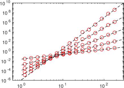
Figure 2: Dimensionless moments of velocity gradients. Symbols from simulations in Ref. [1]. Dashed lines are the theoretical predictions.

and seek the large-$Re$ solution of the form:

$$M_{2n}^{>}=\overline{(\partial_{x}v_{x})^{2n}}\propto(\frac{v_{0}}{L})^{2n}Re^{\rho_{2n}}$$ (10)

Multiplying (10) by $\nu^{n}$ gives:

$$(\frac{L}{v_{0}^{3}})^{n}\overline{{\cal E}^{n}}=Re^{d_{n}}=Re^{\rho_{2n}-n}$$ (11)

leading to the relation between scaling exponents $d_{n}$ and $\rho_{2n}$:

$$\rho_{2n}=d_{n}+n$$ (12)

obtained above. This relation, which is is a consequence of the energy conservation law in the flow driven by white-in-time random force, was studied in Ref. [10]. However, the forcing in [10] was not white-in-time. To stay closer to the theory, here we present results from high-fidelity direct numerical simulations (described below), with a white-in-time forcing scheme.

VI. Scaling exponents. As follows from the definition (3), at a transition point of the $n^{th}$ moment, the large-scale Reynolds number is:

$$Re^{tr}_{n}=C(\hat{R}^{tr}_{\lambda,n})^{\frac{1}{\frac{d_{n}}{n}+\frac{3}{2}}}$$ (13)

Since $R_{1}^{tr}\approx 100-200$, $d_{1}=0$ (see below) and $R^{tr}_{\lambda,1}\approx 8.91$, we obtain an estimate $C\approx 50-100$.

The matching condition at the transition Reynolds number, can now be written as

$$\frac{\overline{{\cal E}^{n}}}{\overline{\cal E}^{n}}=(2n-1)!!=C^{d_{n}}(\hat{R}^{tr}_{\lambda,n})^{\frac{nd_{n}}{d_{n}+\frac{3n}{2}}}$$ (14)

which is a closed equation for the anomalous exponents $d_{n}$. For $n=1$, the left side of relation (14) is equal to unity, giving $d_{1}=0$ and the normalized dissipation rate $\overline{{\cal E}}=1$, consistent with the Navier-Stokes dynamics.

Using large-scale numerical simulations, it has recently been shown that, as discussed above, while the large-scale transitional Reynolds number $Re_{n}^{tr}$ depends on the moment order $n$, the one based on a the $\hat{v}(2n,n)$ field, is independent of $n$ [1] with a value of $\hat{R}^{tr}_{\lambda,n}\approx 9.0$ . This result can be readily understood in terms of the dynamics of transition to turbulence which is not a statistical feature but a property of each realization where $R_{\lambda}>R^{tr}_{\lambda}$. In other words all fluctuations with “local” $\hat{R}_{\lambda,n}\geq Re^{tr}\approx 9.0$ undergo transition to turbulence. This argument, consistent with Landau’s theory of transition, fixes the amplitude in relations (14)-(15) and enables evaluation of the scaling exponents by matching two different flow regimes. Taking $\ln 8.91\approx 2.19$ gives:

$$d_{n}=-\frac{1}{2}[n(\frac{2.19}{\ln C}+\frac{3}{2})-\frac{\ln(2n-1)!!}{\ln C}]+$$

$$\sqrt{\frac{1}{4}[n(\frac{2.19}{\ln C}+\frac{3}{2})-\frac{\ln(2n-1)!!}{\ln C}]^{2}+\frac{3}{2}n\frac{\ln(2n-1)!!}{\ln C}}$$ (15)

where we must use the representation: $(2n-1)!!=\frac{2^{n}}{\sqrt{\pi}}\Gamma(n+\frac{1}{2})$ valid for non-integer values of $n$. This expression is plotted in figure 3a for $n\leq 6$. In part b of the figure we show that for $n\gg 1$, the exponents approach the asymptotic behavior $d_{n}\rightarrow 0.19n\ln n$.

$d_{n}$	$T1$	$DNS$	$C90$	$Exp.$
$d_{1}$	$0.00$	$0.00$	$0.00$	$0.00$
$d_{2}$	$0.158$	$0.149$	$0.187$	$0.152$
$d_{3}$	$0.49$	$0.443$	$0.46$	$0.4$
$d_{4}$	$0.94$	$0.89$	$0.80$	$0.73$
$d_{5}$	$1.49$	$1.47$	$1.19$	$1.1$

Table 2: Comparison of theoretical predictions for exponents $d_{n}$, given by relation (15), with experimental data, semi-empirical models and numerical simulations: $T1$: Theory [10]; $DNS$; present direct numerical simulations; $MF$: multi-fractal theory [10]; $C90$: equation (15) with $\ln[C]=4.5$; Exp.: $d_{n}$ from (15 with $n!$ instead of $(2n-1)!!$ for the Low-Re moments.

$\rho_{n}$	$MF$	$C90$	$DNS2$
$\rho_{1}$	$0.474$	$0.46$	$0.455$
$\rho_{3}$	$1.57$	$1.58$	$1.478$
$\rho_{4}$	$2.19$	$2.19$	$2.05$
$\rho_{5}$	$2.84$	$2.82$	$2.66\pm 0.14$
$\rho_{7}$	$4.20$	$4.13$	$3.99\pm 0.65$

Table 3: Comparison of exponents $\rho_{2n}=d_{n}+n$ with the outcome of numerical simulations and semi-empirical models. $MF$ and $DNS2$: multi-fractal theory and numerical simulations [10]; $C90$: expression (15) with the constant $C=90.$

Evaluation of exponents $\zeta_{n}$. From (15) one obtains $\rho_{1}=0.46$ and, using the relation

$$\rho_{2n}=2n+\frac{\zeta_{4n}}{\zeta_{4n}-\zeta_{4n+1}-1}$$

with $\zeta_{3}=1$, (see Ref.[10]), gives $\zeta_{2}\approx 0.699$ which is different from Kolmogorov’s $\zeta_{2}=2/3$. We would like to point out that the derivation here is not based on geometrical considerations of e.g. the dissipation field, and typically removed from the governing equations. Instead our analysis is based on an exact asymptotic state at low $Re$ and a well established asymptotic state at high $Re$. In this sense is that we believe this to be a derivation first of its kind. In general,

$$\nu^{n}\overline{(\partial_{x}v)^{2n}}=\nu^{n}\overline{(\frac{\delta_{\eta}v}{\eta})^{2n}}\approx\nu^{-n}\overline{(\delta_{\eta}v)^{4n}}\propto Re^{n}\eta^{\zeta_{4n}}_{4n}=Re^{n+\frac{\zeta_{4n}}{\zeta_{4n}-\zeta_{4n+1}-1}}\approx Re^{d_{n}}$$ (16)

with $d_{n}$ evaluated above. Thus, we obtain a recursion relation:

$$\zeta_{4n+1}=\zeta_{4n}F[n]-1$$ (17)

where

$$F[n]=1-\frac{1}{d_{n}-n}$$ (18)

subject to initial condition $\zeta_{2}=0.699$, derived above. The solution for $n\leq 14$ is shown on Table III.

Comparison with direct numerical simulations. In Figure 2 and Table II, we compare the exponents obtained with new high-fidelity direct numerical simulations (DNS) of the Navier-Stokes equations forced at low-wavenumbers with Gaussian white-noise. The accuracy of the simulations have been tested through grid convergence in both space and time. In order to meaningfully compare with the theory, the characteristic length and velocity scales must be independent of the Reynolds number. In general, the root-mean-square velocity or the integral length do present $Re$-dependences, even if weakly, in practical simulations. Thus, we use instead velocity and length scales defined by the independent forcing ${\bf f}$ in (4) using its spectrum $E_{f}(k)$. We then compute the variance of the forcing $\overline{f^{2}}=\int E_{f}(k)dk$ and a length scale $L_{f}=\int E_{f}(k)k^{-1}dk/\overline{f^{2}}$. Finally a velocity scale can be defined as $u_{f}=\sqrt{3}\overline{f^{2}}^{1/4}L_{f}^{1/2}$. We have verified these to be indeed independent of Reynolds number and of the same order of magnitude as the more traditional integral length scale and the root-mean-square of the velocity field. The so normalized gradients are shown in Fig. 2 where we see a wide scaling range where exponents $\rho_{n}$ can be obtained as best fits (dashed lines). The excellent agreement is seen in Table II. In Table III we also see good agreement with the popular multi-fractal formalism and other numerical simulations.

$n$	$1$	$2$	$3$	$4$	$5$	$6$	$7$	$8$	$9$	$10$	$11$	$12$	$13$	$14$
$\zeta_{n}(T)$	$0.369$	$0.699$	$1.0$	$1.26$	$1.53$	$1.78$	$2.07$	$2.29$	$2.56$	$2.84$	$3.14$	$3.47$	$3.85$	$4.27$
$\zeta_{n}(SA)$	$xx$	$0.7$	$1.0$	$1.25$	$xx$	$1.8$	$2.0$	$2.2$	$2.3$	$2.5$

Table 4: Scaling exponents $\zeta_{n}$ of velocity structure functions $S_{n}\propto r^{\zeta_{n}}$. (T): Theory developed in this paper; (SA): exponents from Sreenivasan and Antonia [5]. $xx$ stands for missing data.

Kolmogorov’s Theory. The Kolmogorov’s exponents $\zeta_{n}=n/3$ are obtained from the above theory for a finite moment order $n$ in the limit $\ln C\rightarrow\infty$. As follows from (15), in this case $d_{n}=0$ and the relations (16)-(18) give Kolmogorov’s exponents $\zeta_{n}=n/3$.

Figure 3: Anomalous exponents $d_{n}$ of the moments of dissipation rate $\overline{{\cal E}^{n}}/\overline{{\cal E}}^{n}\propto Re^{d_{n}}$ given by formula (15). (a) $d_{n}$ for $n\leq 6$. (b) High-$n$ limit showing ${5.2d_{n}}/{n\ln n}\rightarrow 1$.

VII. Summary and Conclusions. 1. This paper is based on equations (5)-(7) leading to the well-defined Gaussian low-order moments of velocity derivatives and increments. In this case, transition to strong turbulence is defined as a first appearance of anomalous scaling exponents of the moments of the dissipation rate. No inertial range enters the considerations.
2. In the spirit of Landau’s theory of transition, it is assumed and numerically supported in [1] that in each statistical realization the transition occurs at $\hat{R}_{\lambda,n}\geq 9$ independent on $n$. The numerical value of transitional Reynolds number $R_{\lambda}\approx 8.908$ was derived in Refs. [12-14]. Also, this result comes out of semi-empirical theories of large-scale turbulence modeling [14].
3. We speculate that these two very strong dynamic constraints are satisfied by the formation of small-scale coherent structures manifested by intermittency (anomalous scaling) of dissipation fluctuations in turbulence. In addition, the theory yields an energy spectrum $E(k)\propto k^{-1.699}$.
4. The universality of these results is yet to be studied. On one hand, there has been recent support from numerical and experimental data of various flows [10,16-17]. On the other hand, as we see from Table. 1, numerical values of exponents $d_{n}$ may be sensitive to statistics of the low-Reynolds number fluctuations.
One argument in favor of broad universality can be found in Ref. [8], (Model C), where dynamic renormalization group was applied to the problem of the Navier-Stokes equations driven by various random forces. The authors considered a general force (5) of an arbitrary statistics, supported in a finite interval of wave-numbers $k\approx k_{f}$ and showed that in the limit $k<<k_{f}$ the velocity fluctuations, generated by the model, obeyed Gaussian statistics. This result can be readily understood: each term of the perturbation expansion of (5)-(7) is $O(k^{2n})$. Therefore, in the limit $k\rightarrow 0$, all high-order contributions with $n>1$ disappear as small. This situation corresponds to weak coupling. It is not yet clear how universal this result is.
5. The relation (15) for anomalous exponents $d_{n}$ is a consequence of the coupling of dissipation rate and the random fluctuations of transitional Reynolds numbers (coupling constant) studied in Ref. [1]. The present paper is the first where the role of randomness of a transition point itself in the dynamics of small-scale velocity fluctuations has been addressed. It may be of interest to incorporate this feature in the field-theoretical approaches, like Wyld’s diagrammatic expansions applied to the Navier-Stokes equations for small-scale fluctuations.
6. In this paper anomalous exponents of moments of velocity derivatives and those of dissipation rate have been calculated without introducing any adjustable parameters.
7. It has been shown in [1] that in the limit of a large moment order $n\gg 1$ the transition to strong turbulence, described in this paper, occurs for $\hat{R}_{\lambda,n}^{tr}\approx 9.0$ and $R_{\lambda}\geq 3$. The impact of this constraint on numerical values of the exponents $\zeta_{n}$ in the limit $n\rightarrow\infty$ will be investigated in a future communication.

- (1) 2. C. Lissandrello, K.L. Ekinci and V. Yakhot, “Noisy transitional flows in imperfect channels”, J. Fluid Mech, 778, R3 (2015).
- (2) 3. Kuz’min and Patashinskii, Small Scale Chaos at Low Reynolds Numbers”, Preprint 91-20, Novosibirsk, (1991); Sov. Phys. JETP49, 1050 (1979).
- (3) 4. R.P. Feynman, “The Feynman Lectures on Physics”, Addison Wesley Publishing, 1965. Many sources attribute to Feynman the following statement: “… turbulence is the last unsolved problem of classical physics.” It was pointed out by G. Eyink that the original source of this statement has not been discovered.
- (4) 5. Monin and Yaglom, “Statistical hydrodynamics”, MIT Press, 1975; U. Frisch, “Turbulence”, Cambridge University Press, 1995; Sreenivasan & Anotnia, “The phenomenology of small-scale turbulence”, Ann. Rev. Fluid Mech.
- (5) 6. A. Polyakov, Sov. Phys. JETP, 32, 296 (1971); “Lectures Given at International School on High Energy Physics in Erevan”, 23 November-4 December, (1971);
- (6) 7. L.D. Landau and E.M. Lifshitz, “Fluid Mechanics”, Pergamon, New York, (1982).
- (7) 8. D. Forster, D. Nelson and M.J. Stephen, “Large-distance and long-time properties of a randomly stirred fluid”, Phys. Rev. A 16, 732 (1977).
- (8) 9. H.W. Wyld, “Formulation of the theory of turbulence in an incompressible fluid”, Ann. Phys. 14, 143 (1961).
- (9) 10. J. Schumacher, K.R. Sreenivasan and V. Yakhot, “Asymptotic exponents from low-Reynolds-number flows”, New J. of Phys. 9, 89 (2007).
- (10) 11. D.A. Donzis, P.K. Yeung and K.R. Sreenivasan, “Dissipation and enstrophy in isotropic turbulence: scaling and resolution effects in direct numerical simulations”, Phys. Fluids 20, 045108 (2008).
- (11) 12. V. Yakhot and L. Smith, “The renormalization group, the -expansion and derivation of turbulence models”, J. Sci. Comp. 7, 35 (1992).
- (12) 13. V. Yakhot, Phys. Rev. E, “Reynolds number of transition and self-organized criticality of strong turbulence”, 90, 043019 (2014).
- (13) 14. V. Yakhot, S.A. Orszag, T. Gatski, S. Thangam and C. Speciale, “Development of turbulence models for shear flows by a double expansion technique”, Phys. Fluids A4, 1510 (1992); B.E. Launder and D.B. Spalding, “Mathematical Models of Turbulence”, Academic Press, New York (1972); B.E. Launder and D.B. Spaulding, “The numerical computation of turbulent flows”, Computer Methods in Applied Mechanics and engineering, 3, 269 (1974).
- (14) 15. P.E. Hamlington, D. Krasnov, T. Boeck and J. Schumacher, “Local dissipation scales and energy dissipation-rate moments in channel flow”, J. Fluid. Mech. 701, 419-429 (2012).
- (15) 16. J. Schumacher, J.D. Scheel, D. Krasnov, D.A. Donzis, V. Yakhot and K.R. Sreenivasan, “Small-scale universality in fluid turbulence”, Proc. Natl. Acad. Sci. USA 111, 10961-10965 (2014).
- (16) 17. H. Chen et al., “Extended Boltzmann Kinetic Equation for Turbulent Flows”, Science, 301 , 633 (2003).
- (17)