$p-$forms non-minimally coupled to gravity in Randall-Sundrum scenarios

Abstract

In this paper we study the coupling of $p$-form fields with geometrical tensor fields, namely Ricci, Einstein, Horndeski and Riemann in Randall-Sundrum scenarios with co-dimension one. We consider delta-like and branes generated by a kink and a domain wall. We begin by a detailed study of the Kalb-Ramond (KR) field. The analysis of KR field is very rich since it is a tensorial object and more complex non-minimal couplings are possible. The generalization to $p$-forms can provide more information about the properties and structures that can possibly be universal in the geometrical localization mechanism. The zero mode is treated separately and conditions for localization of zero modes of $p-$forms are found for all the cases above and with this we arrive at the above conclusion about vector fields. Another property that can be tested is the absence of resonances found in the case of vector fields. For this we analyze the possible unstable massive modes for all the above cases via transmission coefficient. Our conclusion is that we have more probability to observe massive unstable modes in the Ricci and Riemann coupling.

1 Introduction

Since Kaluza and Klein introduced extra dimensions in high energy physics to unify electromagnetism and gravitationKaluza:1984ws ; Klein:1926tv , it has been the subject of many developmentsBailin:1987jd . In order to recover the four dimensional physics it was imposed that the extra dimension should be compact. However, at the end of the last century, Randall and Sundrum (RS) proposed an alternative to compactification using the concept of brane-wordsRandall:1999vf . In this scenario the extra dimension is not compact and gravity is trapped to the four dimensional membrane by the introduction of a non-factorisable metric. Since the extra dimension is not compact all the matter fields, and not only gravity, must be trapped on the brane to provide a realistic model. However unlike gravity and the scalar field, the vector field is not trapped on the brane, what becomes a drawback to the RS model. To circumvent this problem some authors introduces a dilaton couplingKehagias:2000au , while others proposes that a strongly coupled gauge theory in five dimensions can generate a massless photon in the braneDvali:1996xe . Most of these models introduces other fields or nonlinearities to the gauge fieldChumbes:2011zt . Some years ago Ghoroku et al proposed a mechanism that does not includes new degrees of freedom and trap the gauge field to the membrane. This is based on the addition of two mass terms, one in the bulk and another on the braneGhoroku:2001zu . Despite working, the mechanism has the undesirable feature of possessing two free parameters, from which one is left after imposing the boundary conditions. Beyond this, the mechanism is not covariant since in principle it introduces a four dimensional mass term which does not come from the five dimensional bulk.

An important point about the presence of more extra dimensions is that it provides the existence of many antisymmetric tensor fields. In five dimensions for example we have the two, three, four and five forms. From the physical viewpoint, they are of great interest because they may have the status of fields describing particles other than the usual ones. As an example we can cite the spacetime torsionMukhopadhyaya:2004cc and the axion fieldArvanitaki:2009fg ; Svrcek:2006yi that have separated descriptions by the two-form. Besides this, String Theory shows the naturalness of higher rank tensor fields in its spectrumPolchinski:1998rq ; Polchinski:1998rr . Other applications of these kind of fields have been made showing its relation with the AdS/CFT conjectureGermani:2004jf . In the RS scenario much has been considered on these tensors. Localization of the zero mode of $p-$forms in delta like branes was first studied in Ref.Kaloper:2000xa where it was claimed that, in $D$ spacetime dimensions, only forms with $p<(D-3)/2$ have a zero mode localized. However, it is well known that in the absence of a topological obstruction, the field strength of a $p-$form is Hodge dual to the $(D-p-2)-$formDuff:1980qv . Using this property is was shown that in fact only for the $0-$form and its dual, the $(D-2)-$form, the fields are localizedDuff:2000se ; Hahn:2001ze . Recently the authors of RefsFu:2015cfa ; Fu:2016vaj showed that this is also related to the gauge fixing of the form fields. This make the problem of localization worse, since the vector field is not localized for any spacetime dimension. Beyond the zero mode, massive modes are important to be considered. Despite the fact that they are not localized, unstable massive modes can be found over the brane by using, for example, the transfer matrix methodLandim:2011ki ; Landim:2011ts ; Alencar:2012en ; Mendes:2017hmv . Resonances of form fields has been found to exist for thick and thin branesAlencar:2010mi ; Alencar:2010hs ; Alencar:2010vk ; Landim:2010pq ; Zhong:2010ae ; Fu:2011pu ; Fu:2012sa ; Fu:2013ita ; Du:2013bx . Recently the Ghoroku mechanism was used to trapp the zero mode of $q-$form fieldJardim:2014vba . The point is that the introduction of the mass terms break the Hodge duality and the argument of Refs.Duff:2000se ; Hahn:2001ze ; Fu:2015cfa ; Fu:2016vaj is not valid anymore. However this solution keeps the above cited undesired features of the Ghoroku mechanism.

In order to solve the above issues, recently a new proposal called ”geometrical localization mechanism” was bornAlencar:2014moa ; Zhao:2014iqa . Looking for a covariant version of the Ghoroku mechanism some of the present authors found that both mass terms can be obtained from a bulk action if the Ricci scalar is coupled to a quadratic mass term of the gauge fieldAlencar:2014moa . Beyond solving the covariantization problem, it also eliminated from the beginning one of the free parameters. The last one is fixed by the boundary conditions leaving no free parameters in the model. The mechanism also keep the advantage of do not adding any new degrees of freedom. Another good property is that it provides the trapping of the gauge fields for any smooth version of the RS scenarioAlencar:2014moa . Soon latter many developments of the idea was put forward. The same non-minimal coupling with the Ricci scalar was proven to work for $q-$forms and ELKO spinors fieldsAlencar:2014fga ; Jardim:2014cya ; Jardim:2014xla . For non-abelian gauge fields it has been found that the non-minimal coupling with the field strength used in Ref.Horndeski:1976gi ; Germani:2011cv should also be introduced and the mechanism worksAlencar:2015awa . A phenomenological prevision of the model has been found for branes with cosmological constant different of zero: a precise residual mass of the photon must exist and this is proposed to be a probe to extra dimensionsAlencar:2015rtc . Recently the same mechanism was shown to emerge from a conformal hidden symmetry of the Randal-Sundrum modelAlencar:2017dqb ; Alencar:2017vqd . In this new scenario fermions are shown to be universally trapped to the membrane by adding a non-minimal coupling with torsion. A new phenomenological prevision was found: a minimum value for the torsion of the membraneAlencar:2017dqb . Soon latter a smooth version of the model was constructed in Alencar:2017vqd . Despite providing the solution to the localization problem, the mechanism raises some questions. When the non-minimal couplings to gauge fields was generalized to includes the Ricci and the EinsteinAlencar:2015oka , it has been found that the last one do not provides a localized solution. The coupling with metric tensor also do not provides a localized zero model and this suggests that tensors with null divergence do not provide a trapped gauge field. When massive modes are considered, a curious result is that for all smooth versions considered no resonances was found. This raises the question if this is an universal property of the mechanismJardim:2015vua .

In this paper we study the coupling of the Kalb-Ramond(KR) field with tensor fields. The analysis of this field is very rich since it is a tensorial object and more complex non-minimal couplings are possible. Beyond the above cited importance of the KR fields, this generalization can provide more information about the properties and structures that can possibly be universal in the geometrical localization mechanism. This paper is organized as follows. In the second section we make a briefly review the RS scenario in co-dimension one. In section III we study the localization of the zero mode of KR field coupled to Ricci, Einstein, Horndeski and Riemann tensors. In the section four we study the possible existence of unstable massives modes for KB field coupled to Ricci, Einstein, Horndeski and Riemann tensors in a RS, kink and domain wall scenarios. In the section five we study the localization of the zero mode of the $p-$form field coupled to Ricci, Einstein, Horndeski and Riemann tensors. In the six section we study the possible existence of unstable massive modes of the $p-$form field coupled to Ricci, Einstein, Horndeski and Riemann tensors in a RS, kink and domain wall scenarios. Finally, in the conclusions we discuss the results.

2 Co-dimension one Randall-Sundrum Scenario

Due to the variety of geometrical objects needed in this manuscript, in this section we briefly review the RS scenario in co-dimension one brane world in $D$-dimensional space-time and construct explicitly all the geometric tensors needed. The coordinates of the whole space-time are $x^{M}$, $M=0,1,2,\cdots D-1$ with $x^{D-1}\equiv z$ the coordinate transverse to the brane and $x^{\mu},\mu=0,1,2,\cdots,D-2$ is the usual Minkowski coordinates. The metric is $ds^{2}=\mbox{e}^{2A(z)}\eta_{MN}dx^{M}dx^{N}$ where $\eta_{MN}=\mbox{diag}(-++\cdots+)$ and the equations of motion are given by Randall:1999vf

$$\sqrt{-G}\left(R_{MN}-\frac{1}{2}G_{MN}R\right)=-\frac{1}{4M^{3}}\left(\Lambda\sqrt{-G}G_{MN}+V\sqrt{-g}g_{\mu\nu}\delta_{M}^{\mu}\delta_{N}^{\nu}\delta(z)\right),$$

where $\Lambda$ is the cosmological constant and $V$ is the brane tension. The conformal form of the metrics provides a simple way to obtain the needed geometrical quantities. Interestingly this will also provide a covariant description of the model. First we must remember that, under a conformal transformation $\tilde{g}_{MN}=\mbox{e}^{2\varphi}g_{MN}$, we have for the Christoffel symbols

$$\tilde{\Gamma}^{K}{}_{IJ}=\Gamma^{K}{}_{IJ}+\delta_{I}^{K}\partial_{J}\varphi+\delta_{J}^{K}\partial_{I}\varphi-g_{IJ}\partial^{K}\varphi.$$

The transformation of the Ricci tensor and Ricci scalar are

$$\tilde{R}_{IJ} = R_{IJ}-(D-2)\left[\nabla_{I}\partial_{J}\varphi-\partial_{I}\varphi\partial_{J}\varphi\right]-\left(\square\varphi+(D-2)\|\nabla\varphi\|^{2}\right)g_{IJ};$$

$$\tilde{R} = \mbox{e}^{-2\varphi}\left(R-2(D-1)\square\varphi-(D-2)(D-1)\|\nabla\varphi\|^{2}\right),$$

where $\nabla_{I}$ is the covariant derivative. From these we can get the transformation of the Einstein tensor, given by

$$\tilde{G}_{IJ}=G_{IJ}-(D-2)\left[\nabla_{I}\partial_{J}\varphi-\partial_{I}\varphi\partial_{J}\varphi\right]+(D-2)\left[\square\varphi+\frac{(D-3)}{2}\|\nabla\varphi\|^{2}\right]g_{IJ}.$$ (1)

In the RS case we have $g_{MN}=\eta_{MN}$ and $\varphi=A(z)$ and this gives us for the components of the Christoffel symbols

$$\Gamma_{D-1\,D-1}^{D-1}=A^{\prime},\Gamma_{\mu\nu}^{D-1}=-A^{\prime}\eta_{\mu\nu,}\Gamma_{D-1\,\alpha}^{\mu}=\delta_{\alpha}^{\mu}A^{\prime}.$$

For the components of the Ricci scalar, Ricci and Einstein tensors we have

$$R=-(D-1)\mbox{e}^{-2A}(2A^{\prime\prime}+(D-2)A^{\prime 2}),$$

$$R_{D-1\,D-1}=-(D-1)A^{\prime\prime},R_{\mu\nu}=-\eta_{\mu\nu}(A^{\prime\prime}+(D-2)A^{\prime 2}),$$

$$G_{D-1\,D-1}=(D-2)(D-1)A^{\prime 2}/2,G_{\mu\nu}=(D-2)(A^{\prime\prime}+\frac{(D-3)}{2}A^{\prime 2})\eta_{\mu\nu}.$$ (2)

With the above results we get for the Einstein equations

$$(D-2)A^{\prime\prime}+\frac{1}{2}(D-2)(D-3)A^{\prime 2} = -\frac{V}{4M^{3}}\delta(z)-\frac{\Lambda}{4M^{3}}\mbox{e}^{2A}$$

$$\frac{1}{2}(D-1)(D-2)A^{\prime 2} = -\frac{\Lambda}{4M^{3}}\mbox{e}^{2A}$$ (3)

with solution

$$A(z)=-\ln(k|z|+1),V=8M^{3}k(D-2),\Lambda=-2M^{3}(D-1)(D-2)k^{2}.$$

Therefore we see that the solution is identical as in the five dimensional case but with the tension of the brane and the cosmological constant depending on the spacetime dimension.

It is important to point that in this manuscript, non-minimal couplings with quadratic higher order antisymmetric tensors will be considered. Therefore we must look for higher order geometric tensors which has the same symmetries. The first geometric tensor of order four with this properties is the Riemann tensor. Under a conformal transformation it changes to

$$\tilde{R}_{IJKL}=\mbox{e}^{2\varphi}\left(R_{IJKL}-\left[g\odot\left(\nabla\partial\varphi-\partial\varphi\partial\varphi+\frac{1}{2}\|\nabla\varphi\|^{2}g\right)\right]_{IJKL}\right),$$

where $\odot$ is the Kulkarni–Nomizu product defined by

$$\left(h\odot k\right)_{IJKL}=h_{IK}k_{JL}+h_{JL}k_{IK}-h_{IL}k_{JK}-h_{JK}k_{IL}.$$

When considering the RS metrics the components are simplified to

$$R_{\mu\nu\alpha\,D-1}=0,R_{\mu\,D-1\nu\,D-1}=-\eta_{\mu\nu}(A^{\prime\prime}+2A^{\prime 2})\mbox{e}^{2A},R_{\mu\nu\alpha\beta}=-A^{\prime 2}\mbox{e}^{2A}(\eta_{\mu\alpha}\eta_{\nu\beta}-\eta_{\nu\alpha}\eta_{\mu\beta}).$$ (4)

However, the curvature tensor has non-null divergence. As said in the introduction, we must also analyze tensors with null divergence. A fourth order tensor with this property is the Horndeski tensor and has been coupled to the field strength of the vector field Ref.Horndeski:1976gi ; Germani:2011cv ; Alencar:2015awa . Curiously this tensor has all the desired symmetries. Here we will consider the coupling this tensor to the mass term of the form field. It is given by

$$\Delta^{AB}{}_{CD}\equiv\frac{1}{8}R^{AB}{}_{CD}-\frac{1}{2}R^{[A}{}_{[C}\delta^{B]}{}_{D]}+\frac{1}{8}R\delta^{[A}{}_{[C}\delta^{B]}{}_{D]},$$

where

$$M^{[A}{}_{[C}N^{B]}{}_{D]}\equiv\frac{1}{4}(M^{A}_{C}N^{B}_{D}-M^{A}_{D}N^{B}_{C}+M^{B}_{D}N^{A}_{C}-M^{B}_{C}N^{A}_{D}).$$

We should point that, since it has null divergence in any index, after contracting two of them we must obtain a tensor proportional to the Einstein tensor. In fact, by a direct calculation we get

$$\Delta^{AB}{}_{CB}=-\frac{D-3}{8}G^{A}_{C}.$$

Under a conformal transformation we have

$$\tilde{\Delta}^{AB}{}_{CD}=\Delta^{AB}{}_{CD}-\mbox{e}^{-2\varphi}(D-3)\mathcal{H}^{AB}_{CD},$$

where

$$\mathcal{H}^{AB}_{CD}=\left(\frac{1}{4}\square\varphi+\frac{(D-4)}{8}(\nabla\varphi)^{2}\right)\delta^{[A}{}_{[C}\delta^{B]}{}_{D]}-\frac{1}{2}\left(\delta_{[C}^{[A}\partial^{B]}\partial_{D]}\varphi-\delta_{[C}^{[A}\partial^{B]}\varphi\partial_{D]}\varphi\right).$$

Using the RS metrics we obtain the components

$$\Delta^{\mu\nu}{}_{\alpha\beta}=-\frac{\mbox{e}^{-2A}}{8}(D-3)(\delta_{\alpha}^{\mu}\delta_{\beta}^{\nu}-\delta_{\beta}^{\mu}\delta_{\alpha}^{\nu})(A^{\prime\prime}+\frac{(D-4)}{2}A^{\prime 2}),$$

and

$$\Delta_{\nu\,D-1}^{\mu\,D-1}=-\frac{\mbox{e}^{-2A}}{16}\delta_{\nu}^{\mu}(D-3)(D-2)A^{\prime 2}.$$

We will use the above results to study a variety of geometrical couplings which can renders localized modes for the fields. First we will study zero mode localization and then the massive modes. In the section 3 we will restrict our analysis to five dimensional case.

3 The Kalb-Ramond zero mode case

In this section we will make a direct generalization of the geometric coupling, presented in Ref.Alencar:2015oka , for the KR field. This is gonna be a prototype for the due generalization to the $q-$form field in the section five. Beyond this, due to its importance it is worthwhile to make a separate study. We will consider the coupling to tensors of order two and four.

3.1 Kalb-Ramond coupled with a rank two geometric tensor

In this subsection we will consider the coupling of the KR field to rank two geometric tensors. The action is given by

$$S=-\int d^{5}x\sqrt{-g}\left[\frac{1}{12}Y_{M_{1}M_{2}M_{3}}Y^{M_{1}M_{2}M_{3}}+\frac{1}{2}\gamma g_{N_{1}N_{2}}H_{M_{1}M_{2}}X^{M_{1}N_{1}}X^{M_{2}N_{2}}\right],$$ (5)

where $X_{MN}$ is the anti-symmetric Kalb-Ramond two form field and $Y_{MNO}=\partial_{[M}X_{NO]}$. We also use $H_{M_{1}M_{2}}$ as a generic rank two geometric tensor and $\gamma$ is a coupling constant. The above action provides the following equation of motion for the KR field

$$\frac{1}{2}\partial_{M_{1}}\left[\sqrt{-g}Y^{M_{1}M_{2}M_{3}}\right]-\gamma\sqrt{-g}g^{N_{1}[M_{3}}H^{M_{2}]M_{1}}X_{M_{1}N_{1}}=0,$$ (6)

and from this, we get the identity

$$\partial_{M_{2}}\left[\sqrt{-g}g^{N_{1}[M_{3}}H^{M_{2}]M_{1}}X_{M_{1}N_{1}}\right]=0.$$ (7)

The analyzes can be simplified if we observe that in all the cases the tensors has the same form, namely

$$H_{\mu\nu}=H_{0}\eta_{\mu\nu},H_{44}=H_{1},$$ (8)

and all other components are null. For a free index equal to extra dimension index, i.e., $M_{3}=4$ we obtain from the equations of motion (6) the vectorial equation

$$\partial_{\mu}Y^{\mu\nu 4}-\gamma(H_{0}+H_{1})X^{\nu 4}=0,$$ (9)

where in the above expression and from now on all the indexes are raised with $\eta^{\mu\nu}$. Taking $M_{3}=\mu_{3}$ in (6) we obtain a tensorial equation

$$\frac{1}{2}\mbox{e}^{-A}\partial_{\mu_{1}}Y^{\mu_{1}\mu_{2}\mu_{3}}+\frac{1}{2}\partial_{z}\left[\mbox{e}^{-A}Y^{4\mu_{2}\mu_{3}}\right]-\gamma\mbox{e}^{-A}{H}_{0}X^{\mu_{2}\mu_{3}}=0.$$ (10)

Taking the free index $M_{3}=4$ in the identity (7), we obtain the gauge condition for the vector field, i.e., $\partial_{\mu_{1}}X^{\mu_{1}4}=0$. For the free index $M_{3}=\mu_{3}$ we obtain a tensorial condition

$$\mbox{e}^{-A}{H}_{0}\partial_{\mu_{1}}X^{\mu_{1}\nu_{1}}+\frac{1}{2}\partial_{z}\left[\mbox{e}^{-A}({H}_{1}+{H}_{0})X^{4\nu_{1}}\right]=0.$$ (11)

Therefore the KR field is not divergence free and we must decompose it as $X^{\mu_{1}\mu_{2}}=X_{L}^{\mu_{1}\mu_{2}}+X_{T}^{\mu_{1}\mu_{2}}$, with

$$X_{T}^{\mu_{1}\mu_{2}}=X^{\mu_{1}\mu_{2}}+\frac{1}{\Box}\partial^{[\mu_{1}}\partial_{\nu_{1}}X^{\mu_{2}]\nu_{1}};\;\;\;\;X_{L}^{\mu_{1}\mu_{2}}=-\frac{1}{\Box}\partial^{[\mu_{1}}\partial_{\nu_{1}}X^{\mu_{2}]\nu_{1}}.$$ (12)

where $X_{T}^{\mu_{1}\mu_{2}}$ has null divergence, as desired. From now on, we must show that the transversal and longitudinal parts of the field decouples in the equations of motion. For this, we first show that from the above definitions we get

$$\partial_{\mu_{1}}Y^{\mu_{1}\mu_{2}\mu_{3}}=2\square X_{T}^{\mu_{2}\mu_{3}};\;\;\;\;Y^{\mu_{1}\mu_{2}4}=Y^{\mu_{1}\mu_{2}4}_{L}+2\partial X^{\mu_{1}\mu_{2}}_{T},$$ (13)

where $Y^{\mu_{1}\mu_{2}4}_{L}\equiv\partial^{\mu_{1}}X^{\mu_{2}4}-\partial^{\mu_{2}}X^{\mu_{1}4}$. Using the above result in the field equations we arrive at

$$\mbox{e}^{-A}\Box X^{\mu_{2}\mu_{3}}_{T}+\partial_{z}\left[\mbox{e}^{-A}\partial_{z}X^{\mu_{2}\mu_{3}}_{T}\right]+\frac{1}{2}\partial_{z}\left[\mbox{e}^{-A}Y^{\mu_{2}\mu_{3}4}_{L}\right]$$

$$-\gamma\mbox{e}^{-A}{H}_{0}X^{\mu_{2}\mu_{3}}_{L}-\gamma\mbox{e}^{-A}{H}_{0}X^{\mu_{2}\mu_{3}}_{T}=0,$$ (14)

$$\partial_{\mu}Y^{\mu\nu 4}_{L}-\gamma({H}_{0}+{H}_{1})X^{\nu 4}=0.$$ (15)

From the definition of $Y^{\mu_{1}\mu_{2}4}_{L}$ we can also show that

$$Y^{\mu_{2}\mu_{3}4}_{L}=-\frac{1}{\Box}\partial^{[\mu_{2}}\partial_{\nu}Y^{\mu_{3}]\nu 4},$$ (16)

and using Eqs.(9), (11) and (12) we can finally show that the longitudinal propagator term that appear in (15) is equal to

$$\partial_{z}\left[\mbox{e}^{-A}Y^{\mu_{2}\mu_{3}4}_{L}\right]=\gamma\partial_{z}\left[\mbox{e}^{-A}({H}_{0}+{H}_{1})\frac{1}{\Box}\partial^{[\mu_{2}}X^{\mu_{3}]4}\right]$$

$$=-2\gamma H_{0}\mbox{e}^{-A}\frac{1}{\Box}\partial^{[\mu_{2}}\partial_{\mu_{1}}X^{\mu_{3}]\mu_{1}}=2\gamma H_{0}\mbox{e}^{-A}X_{L}^{\mu_{2}\mu_{3}}.$$ (17)

The above identity can be used to decouples the fields in Eq. (15), and provides the final equation for the transversal component

$$\mbox{e}^{-A}\Box X^{\mu_{2}\mu_{3}}_{T}+\partial_{z}\left[\mbox{e}^{-A}\partial_{z}X^{\mu_{2}\mu_{3}}_{T}\right]-\gamma\mbox{e}^{-A}{H}_{0}X^{\mu_{2}\mu_{3}}_{T}=0.$$ (18)

Performing the separation of variables in the form $X_{T}^{\mu_{1}\mu_{2}}=\tilde{X}_{T}^{\mu_{1}\mu_{2}}(x)\mbox{e}^{A/2}\psi_{T}(z)$, we obtain the set of equations

$$\Box\tilde{X}^{\mu_{2}\mu_{3}}_{T}-m^{2}_{T}\tilde{X}^{\mu_{2}\mu_{3}}_{T}=0,$$ (19)

$$\psi_{T}^{\prime\prime}-U_{T}(z)\psi_{T}=-m^{2}_{T}\psi_{T},$$ (20)

where the potential is given by

$$U_{T}(z)=\frac{A^{\prime 2}}{4}-\frac{A^{\prime\prime}}{2}+\gamma{H}_{0}.$$ (21)

To decouple the vector field and the longitudinal part of KR field we use the divergence equation (11) in (15). This procedure leads to

$$\Box X^{\nu 4}+\partial_{z}\left[\frac{\mbox{e}^{A}}{2H_{0}}\partial_{z}\left(\mbox{e}^{-A}(H_{0}+H_{1})X^{\nu 4}\right)\right]-\frac{\gamma}{2}(H_{0}+H_{1})X^{\nu 4}=0.$$ (22)

To write the above equation in a Schrödinger-like form we must separate the variables in the form $X^{\nu 4}=\tilde{X}^{\nu}(x)F(z)\psi(z)$, where

$$F(z)=\frac{2\mbox{e}^{A/2}({H}_{0})^{1/2}}{{H}_{0}+{H}_{1}}.$$ (23)

This procedure splits the equation (22) in the following set of equations

$$\Box\tilde{X}^{\nu}-m^{2}\tilde{X}^{\nu}=0$$ (24)

$$\psi^{\prime\prime}-U(z)\psi=-2m^{2}\frac{{H}_{0}}{{H}_{0}+{H}_{1}}\psi,$$ (25)

where the potential of Schrödinger equation is given by

$$U(z)=\frac{1}{4}\left[A^{\prime}-(\ln{H}_{0})^{\prime}\right]^{2}+\frac{1}{2}\left[A-\ln{H}_{0}\right]^{\prime\prime}+\gamma{H}_{0}.$$ (26)

The equations (20) and (25), with the potentials (21) and (26), governs the extra dimension component of KR and vector fields respectively.

Now we must analyze the localization of the zero mode of the KR and vector fields. We first consider the KR case. For this we must to explicit the geometric tensor which couples with KR field in the action (5). We will see that this can be achieved without any specific form for the warp factor. The only condition is that the RS model is recovered for large $z$. First of all, the potential (21) can further be simplified if we note that $H_{0}$ are combinations of $A^{\prime 2}$ and $A^{\prime\prime}$

$$H_{0}=\lambda_{0}A^{\prime\prime}+\beta_{0}A^{\prime 2},H_{1}=\lambda_{1}A^{\prime\prime}+\beta_{1}A^{\prime 2},$$ (27)

what gives us its final form

$$U_{T}(z)=(\frac{1}{4}+\gamma\beta_{0})A^{\prime 2}-(\frac{1}{2}-\gamma\lambda_{0})A^{\prime\prime}.$$ (28)

Supposing now the solution for the zero mode $\psi(z)=\mbox{e}^{\sigma A(z)}$, we obtain from Eq.(20) with $m=0$ the set of algebraic equations

$$\gamma(-\gamma\lambda_{0}^{2}+\lambda_{0}+\beta_{0})=0,$$ (29)

$$\sigma=-(1/2-\gamma\lambda_{0}).$$ (30)

The solution $\gamma=0$ is the solution for the free KR field and gives us a non localized field as expected. For $\lambda_{0}=0$ we have $\gamma\beta_{0}=0$ what also implies the free field solution which is not localized. The last possibility is $\gamma\neq 0$ and $\lambda_{0}\neq 0$. With this we get the solutions

$$\gamma=\frac{\lambda_{0}+\beta_{0}}{\lambda_{0}^{2}},$$ (31)

$$\sigma=1/2+\frac{\beta_{0}}{\lambda_{0}}.$$ (32)

Therefore to obtain a convergent solution for the zero mode of the transversal part of KR field, a necessary condition is that $\beta_{0}/\lambda_{0}>0$. This is valid in all brane scenarios that recover the RS asymptotically.

The first example is the Ricci tensor. From the last section we can see that

$$H_{0}=-(A^{\prime\prime}+3A^{\prime 2}),H_{1}=-4A^{\prime\prime},$$

and therefore $\lambda_{0}=-1,\beta_{0}=-3$, which gives us a localized zero mode if $\gamma=-4$ with $\sigma=7/2$. Therefore, just as in the case for the vector field Alencar:2015oka , the KR field we can be localized with the Ricci tensor. The Einstein tensor is the second example of a rank two geometric tensor. From the last section we can see that in this case

$$H_{0}=3(A^{\prime\prime}+A^{\prime 2}),H_{1}=6A^{\prime 2},$$ (33)

and we have $\lambda_{0}=3,\beta_{0}=3$. This value provides a localized solution for the zero mode of transversal part of KR field for a coupling constant fixed by $\gamma=2/3$ with $\sigma=3/2$.

Next we will analyze the localization of the zero mode of the vector component of the KR field. In this case, due to the transformation (23), the integral that must be finite is given by

$$\int\frac{H_{0}}{(H_{0}+H_{1})^{2}}\psi^{2}dz,$$ (34)

where $\psi$ is the solution of (25) with $m=0$. However, different of the tensor case, it is not possible to find analytical solutions of Eq.(25). However, a necessary condition for localizability is a convergent solution for large $z$. Since all the smooth versions considered here recover RS for large $z$, we can use this solution to test the localizability of the field. With these considerations we can use the Einstein equation (3), which will be valid for large $z$, to obtain that

$$A^{\prime\prime}=A^{\prime 2}=k^{2}e^{2A},$$ (35)

and therefore

$$H_{0}=(\lambda_{0}+\beta_{0})k^{2}e^{2A},H_{1}=(\lambda_{1}+\beta_{1})k^{2}e^{2A}.$$ (36)

From the above relation we get for the potential (26) at large $z$

$$U(z)=\frac{A^{\prime 2}}{4}-\frac{A^{\prime\prime}}{2}+\gamma H_{0}.$$ (37)

This is the same potential found for the KR case, Eq.(21). Therefore the solution is the same, namely $\psi=e^{\sigma A}$, with the same $\sigma$ and $\gamma$ as before. However, since the integrand for the vector case is given by Eq.(34) the condition for localizability is different. In the limit considered here we can use (36) and the integrand of Eq.(34) reduces to $e^{2A}\psi^{2}$. Therefore the condition for localization in this case is given by $\beta_{0}/\lambda_{0}>-1$. By this fact, we can conclude that for any case in which the KR is localized we also have a localized vector field. With this, we show that the hypothesis of Ref.Alencar:2015oka that tensors with null divergence do not trap zero modes is no valid. This is true since the Einstein tensor can localize the KR field.

3.2 Kalb-Ramond coupled with a rank four geometric tensor

In this section we will extend the coupling used in last subsection to a rank four geometric tensor. As said in the first section these tensors must have the same symmetries of the Riemann tensor in order to couple with the quadratic KR field. The action is given by

$$S=-\int d^{5}x\sqrt{-g}\left[\frac{1}{24}Y_{M_{1}M_{2}M_{3}}Y^{M_{1}M_{2}M_{3}}+\frac{1}{4}\gamma H_{M_{1}N_{1}M_{2}N_{2}}X^{M_{1}N_{1}}X^{M_{2}N_{2}}\right],$$ (38)

where $H_{M_{1}N_{1}M_{2}N_{2}}$ is a generic geometric tensor. The equations of motion are

$$\frac{1}{2}\partial_{M_{1}}\left[\sqrt{-g}Y^{M_{1}M_{2}M_{3}}\right]-\gamma\sqrt{-g}H^{M_{1}N_{1}M_{2}M_{3}}X_{M_{1}N_{1}}=0,$$ (39)

and from this we get the constraint

$$\partial_{M2}(\sqrt{-g}H^{M_{1}N_{1}M_{2}M_{3}}X_{M_{1}N_{1}})=0.$$ (40)

Now we proceed to decompose these equations in components. As previously pointed, before this we should note that all tensors considered by us have the following structure

$$H^{\mu_{1}\mu_{2}\mu_{3}\mu_{4}}=\frac{1}{2}\mbox{e}^{-6A}H_{0}(\eta^{\mu_{1}\mu_{3}}\eta^{\mu_{2}\mu_{4}}-\eta^{\mu_{2}\mu_{3}}\eta^{\mu_{1}\mu_{4}}),$$

$$H^{\mu_{1}4\mu_{2}4}=\frac{1}{2}\mbox{e}^{-6A}H_{1}\eta^{\mu_{1}\mu_{2}},$$

$$H^{\mu_{1}\nu_{1}4\mu_{3}}=H^{\mu_{1}4\mu_{2}\mu_{3}}=0.$$ (41)

With this, we obtain from Eq.(39) with $M_{2}=\mu_{2},M_{3}=\mu_{3}$ and $M_{3}=4$ respectively

$$\frac{1}{2}\mbox{e}^{-A}\partial_{\mu_{1}}\left[Y^{\mu_{1}\mu_{2}\mu_{3}}\right]+\frac{1}{2}\partial_{z}\left[\mbox{e}^{-A}Y^{4\mu_{2}\mu_{3}}\right]-\gamma H_{0}\mbox{e}^{-A}X^{\mu_{2}\mu_{3}}=0,$$ (42)

$$\frac{1}{2}\partial_{\mu}Y^{\mu\nu 4}-\gamma H_{1}X^{\nu 4}=0,$$ (43)

and for the constraint (40) we get the following components

$$\partial_{z}\left(\mbox{e}^{-A}H_{1}X^{4\mu_{3}}\right)+\mbox{e}^{-A}H_{0}\partial_{\mu_{2}}X^{\mu_{2}\mu_{3}}=0,$$ (44)

$$\partial_{\mu_{2}}X^{\mu_{2}4}=0.$$ (45)

As expected the KR field does not has null divergence and now we proceed to show that its longitudinal and transversal pieces, as defined in Eq.(12), decouples. For this we use the identities (13) in the equations of motion to obtain

$$\mbox{e}^{-A}\Box X^{\mu_{2}\mu_{3}}_{T}+\partial_{z}\left(\mbox{e}^{-A}\partial_{z}X^{\mu_{2}\mu_{3}}_{T}\right)+\frac{1}{2}\partial_{z}\left(\mbox{e}^{-A}Y^{\mu_{2}\mu_{3}4}_{L}\right)$$

$$-\gamma H_{0}\mbox{e}^{-A}X^{\mu_{2}\mu_{3}}_{L}-\gamma H_{0}\mbox{e}^{-A}X^{\mu_{2}\mu_{3}}_{T}=0,$$ (46)

$$\frac{1}{2}\partial_{\mu}Y^{\mu\nu 4}_{L}-\gamma H_{1}X^{\nu 4}=0.$$ (47)

Now, by using the identity (16) and Eqs.(43),(44) and (12) we can show that

$$\partial_{z}\left(\mbox{e}^{-A}Y^{4\mu_{2}\mu_{3}}\right)=2\gamma H_{0}\mbox{e}^{-A}X^{\mu_{2}\mu_{3}}_{L},$$

and the longitudinal contribution decouples in Eq.(3.2). To decouple the vector component we just use Eq.(44) in (47). With this, we finally get for the decoupled equations of motion

$$\mbox{e}^{-A}\Box X^{\mu_{2}\mu_{3}}_{T}+\partial_{z}\left(\mbox{e}^{-A}\partial_{z}X^{\mu_{2}\mu_{3}}_{T}\right)-\gamma H_{0}\mbox{e}^{-A}X^{\mu_{2}\mu_{3}}_{T}=0,$$ (48)

$$\Box X^{\nu 4}+\partial_{z}\left[\frac{\mbox{e}^{-A}}{H_{0}}\partial_{z}\left(\mbox{e}^{A}H_{1}X^{\nu 4}\right)\right]-\gamma H_{1}\mbox{e}^{2A}X^{\nu 4}=0.$$ (49)

For the transversal part of KR field, making the separation $X^{\mu_{2}\mu_{3}}_{T}=\tilde{X}^{\mu_{2}\mu_{3}}_{T}(x)\mbox{e}^{A/2}\psi_{T}(z)$, we obtain

$$\Box\tilde{X}^{\mu_{2}\mu_{3}}_{T}=m^{2}_{T}\tilde{X}^{\mu_{2}\mu_{3}}_{T},$$ (50)

$$\psi_{T}^{\prime\prime}-U_{T}(z)\psi_{T}=-m^{2}_{T}\psi_{T},$$ (51)

where the Schrödinger’s potential is given by

$$U_{T}(z)=A^{\prime 2}/4-A^{\prime\prime}/2+\gamma H_{0}.$$ (52)

To write the vector equation in a Schrödinger-like form we must separate the variables $X^{\nu 4}=\tilde{X}^{\nu}(x)F(z)\psi(z)$, where

$$F(z)=\frac{\mbox{e}^{A/2}({H}_{0})^{1/2}}{{H}_{1}},$$ (53)

and we get

$$\Box\tilde{X}^{\nu}-m^{2}\tilde{X}^{\nu}=0,$$ (54)

$$\psi^{\prime\prime}-U(z)\psi=-m^{2}\frac{{H}_{0}}{{H}_{1}}\psi,$$ (55)

where the potential of Schrödinger equation is given by

$$U(z)=\frac{1}{4}\left[A^{\prime}-(\ln{H}_{0})^{\prime}\right]^{2}+\frac{1}{2}\left[A-\ln{H}_{0}\right]^{\prime\prime}+\gamma{H}_{0}.$$ (56)

At this point we must analyze the localization of the zero modes of the fields. However we can see that the form of the equations that governs the zero modes are identical and in the last section. Therefore, if H decomposes as in (27) we will have that the tensor component is localized for $\lambda_{0}\neq 0$ and $\beta_{0}/\lambda_{0}>0$, with $\gamma$ given by Eq. (31). For the Riemann tensor, by comparing Eq. (4) with Eqs. (3.2) and (27), we have

$$H_{0}=-2A^{\prime 2},H_{1}=-2(A^{\prime\prime}+2A^{\prime 2}),$$ (57)

and therefore $\lambda_{0}=0$. The conclusion is that the Riemann tensor do not trap the KR field. For the Horndeski tensor we have

$$H_{0}=-\frac{1}{2}(A^{\prime\prime}+\frac{1}{2}A^{\prime 2}),H_{1}=-\frac{3}{8}A^{\prime 2},$$ (58)

and $\lambda_{0}=-1/2,\beta_{0}=-1/4$, what gives a localized zero mode with $\gamma=-3$ and $\sigma=1$. Just as before, the vector field is localized always that the KR field is localized. At this point is curious to see that relation with null divergence and localization seems to be inverted. The Horndeski tensor has null divergence and provides a trapped field, while the Riemann tensor do not. In order to obtain a final answer for this questions we have to generalize our results to $p-$form fields. We do this in the next sections, but before we analyze the possible resonances for the cases considered here.

4 Kalb-Ramond massive modes

In this section we study the possible resonant modes with Kalb-Ramond field coupled to Ricci, Einstein, Horndeski and Riemann tensors, through the transmission coefficient. The resonant modes appears when the transmission coefficient $T$ is equal to 1, i.e, $Log(T)=0$. We analyze in three possible scenarios: Randall-Sundrum delta like brane, a brane generated by a domain wall and generated by a kink.

We first observe that for all tensor coupling, the potential of Schrödinger equation in conformal metric has the form

$$U_{T}(z)=\alpha A^{\prime}(z)^{2}+\beta A^{\prime\prime}(z),$$ (59)

where $\beta=\sigma=7/2,3/2,1$, $\alpha=\sigma^{2}$ for Ricci, Einstein and Horndeski tensors respectively and $\alpha=1/4-2\gamma$, $\beta=-1/2$ for the Riemann tensor.

4.1 In Randall-Sundrum delta like scenario

The first brane scenario that we will study is the Randall-Sundrum scenario Randall:1999vf . Despite the singularity this scenario has a historical importance and serves as an important paradigm in physics of extra dimensions and field localization. The warp factor of this scenario in a conformal form is given by

$$A(z)=-\ln\left(k|z|+1\right).$$ (60)

In this scenario, the potential of Schrödinger equation is given by

$$U_{T}(z)=\frac{(\alpha+\beta)k^{2}}{(k|z|+1)^{2}}-2k\beta\delta(z),$$ (61)

and is illustrated in Fig. 1. The regular part of $U_{T}(z)$ has a maximum at $z=0$. For Riemann tensor $\alpha+\beta=-1/4-2\gamma$. We must have $\gamma<-1/8$, in order to provide a positive maximum for the potential and a positive asymptotic behavior.

Figure 1: Plot of regular part of Schrödinger potential for KR field in Randall-Sundrum delta like scenario with $k=1$ and $\alpha+\beta=30$.

For the massive case, the Eq. (20) provides the solution

$$\psi(z)=(k|z|+1)^{1/2}[C_{1}J_{\nu}(m_{T}|z|+m_{T}/k)+C_{2}Y_{\nu}(m_{T}|z|+m_{T}/k)],$$ (62)

where $C_{1}$ and $C_{2}$ are constants with $\nu=\sigma+1/2$ for Ricci, Einstein and Horndeski tensors coupling and $\nu=\sqrt{-2\gamma}$ for Riemann tensor coupling. Since the Bessel functions goes to infinity as $(m_{T}|z|+m_{T}/k)^{-1/2}$, no fixation of constants $C_{1}$ and $C_{2}$ produces a convergent solution. Then the massive modes are non-localized. To obtain more information about massive modes we can evaluate the transmission coefficient. For this, we will write the solution (62) in the form

$$\psi(z)=\left\{\begin{matrix}E_{\nu}(-z)+rF_{\nu}(-z)&,\;\mbox{for}\;z<0\\ tF_{\nu}(z)&,\;\mbox{for}\;z\geq 0\end{matrix}\right.,$$ (63)

where

$$E_{\nu}(z)=\sqrt{\frac{\pi}{2}}(m_{T}z+m_{T}/k)^{1/2}H^{(2)}_{\nu}(m_{T}z+m_{T}/k),$$ (64)

$$F_{\nu}(z)=\sqrt{\frac{\pi}{2}}(m_{T}z+m_{T}/k)^{1/2}H^{(1)}_{\nu}(m_{T}z+m_{T}/k),$$ (65)

$H^{(1)}_{\nu}$ and $H^{(2)}_{\nu}$ are the Hankel functions of first and second kind respectively, $r$ and $t$ are constants. The boundary conditions at $z=0$ imposes

$$t=\frac{W(E_{\nu},F_{\nu})(0)}{2F_{\nu}(0)F_{\nu}^{\prime}(0)+2k\beta F_{\nu}^{2}(0)},$$ (66)

where $W(E_{\nu},F_{\nu})(0)=E_{\nu}(0)F_{\nu}^{\prime}(0)-E_{\nu}^{\prime}(0)F_{\nu}(0)$ is the Wronskian at $z=0$. Since the Wronskian is constant in Schrödinger equation, the transmission coefficient can be written as

$$T=|t|^{2}=\frac{m_{T}^{2}}{|F_{\nu}(0)F_{\nu}^{\prime}(0)+k\beta F_{\nu}^{2}(0)|^{2}}.$$ (67)

The transmission coefficient was plotted in Fig. 2 as function of $E=m_{T}^{2}$ for the KR field in the Ricci, Einstein and Horndeski coupling and does not show peaks, indicating no unstable massive modes. The transmission coefficient was plotted for Riemann coupling in Fig. 2 and does not show peaks, indicating no unstable massive modes.

Figure 2: Transmission coefficient for KR field in Randall-Sundrum delta like scenario with $k=1$ as function of $E=m_{T}^{2}$. (a) Ricci, Einstein and Horndeski tensor coupling, (b) Riemann tensor coupling.

For the vector field in Randall-Sundrum scenario the potential of Schrödinger equation, (26), can be written as

$$U(z)=\frac{(\alpha+\beta)k^{2}}{(k|z|+1)^{2}}-2k\beta\delta(z).$$ (68)

This is the same potential of KR filed, so the behavior of the modes of vector field is the same, i.e., the zero mode is localized while the massive are not. The transmission coefficient for the massive modes is the same of KR field, Figs. 2 and 2.

4.2 In brane scenario generated by a domain-wall

In this section we will use the smooth warp factor produced by a domain-wallDu:2013bx ; Melfo:2002wd ,

$$A(z)=-\frac{1}{2n}\ln\left[\left(kz\right)^{2n}+1\right],$$ (69)

which recover the Randall-Sundrum metric at large $z$ for $n\in N^{*}$.

Using this metric in Eq. (21) we obtain the Schrödinger’s potential for transversal part of KR field

$$U_{T}(z)=\frac{(kz)^{2n}\left(\alpha(kz)^{2n}+\beta\left((kz)^{2n}-2n+1\right)\right)}{z^{2}\left((kz)^{2n}+1\right)^{2}},$$ (70)

which is illustrated in Fig. 3, for Ricci tensor coupling with some values of $n$.

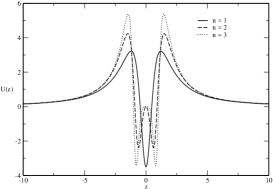
Figure 3: Schrödinger’s potential for KR field in smooth scenario generated by domain walls for Ricci tensor coupling with some values of parameter $n$ and $k=1$.

The solution of massive modes of transversal of KB field can not be found analytically. To obtain information about this state we use the transfer matrix method to evaluate the transmission coefficient. The behavior of the transmission coefficient for Ricci, Einstein and Horndeski coupling is illustrated in Figs. 4, 4 and 4 for some values of parameter $n$. As we can see, for Ricci tensor coupling, resonant peaks appears when we increase the values of the parameter $n$ indicating the existence of unstable massive modes. The same occur for Einstein tensor coupling. In the Horndeski coupling we observe the absence of resonant peaks.

The behavior of the transmission coefficient for Riemann coupling is illustrated in Fig. 5 for some values of parameter $n$ with $\gamma=-2$ and in Fig. 5 for some values of coupling constant $\gamma$ with $n=1$. As we can see, when we increase the values of $n$ and $|\gamma|$ we observe the appearance of resonant peaks, indicating the existence of unstable massive modes.

For the reduced vector field the potential is given by Eq. (26). The components $H_{0}$ and $H_{1}$ vanishes at regular points near to the origin for all values of parameter $n$ and the potential diverges at this same points (see Figs. 6 and 6). These kind of divergence does not allow us to use the transfer matrix method to compute the transmission coefficient and to evaluate the existence of unstable massive modes.

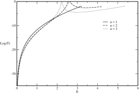
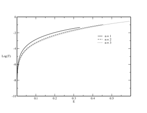
Figure 4: The transmission coefficient in a smooth scenario generated by domain walls for some values of parameter $n$ as function of $E=m_{T}^{2}$. (a) Ricci tensor, (b) Einstein tensor and (c) Horndeski tensor.

Figure 5: Transmission coefficient for KR field in brane scenario generated by domain-walls with Riemann tensor coupling as a function of $E=m_{T}^{2}$. (a) For some values of $n$ with $\gamma=-2$. (b) For some values of coupling constant $\gamma$ with $n=1$.

Figure 6: The components $H_{0}$ and $H_{1}$ in smooth scenario generated by domain wall with $n=1$ for the Ricci, Einstein and Horndeski tensors. (a) $H_{0}$ and (b) $H_{1}$.

4.3 In brane scenario generated by a kink

For a four dimensional brane generated by a kink, the warp factor is given byLandim:2011ki

$$A(y)=-4\ln\cosh y-\tanh^{2}y,$$ (71)

where the variable $y$ relates with the conformal coordinate, $z$, by

$$dz=\mbox{e}^{-A(y)}dy.$$ (72)

The behavior of potential of transversal part of KB field, Eq. (21), with this warp factor is illustrated in Fig. 7 for Riemann coupling. For massive modes, like in previous sections, we use the matrix transfer method to compute the transmission coefficient. The result is plotted in Figs. 8, 8, 9 and 9. As we can see, for Ricci tensor coupling we have a resonant peak near $E=0.5$ and near $E=14$ with $\lambda=-5$ for Riemann coupling.

Figure 7: (a) Schrödinger potential in kink scenario for KR field coupled to Riemann tensor for some values of coupling constant $\gamma$.

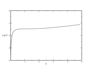
Figure 8: Transmission coefficient in kink scenario for KR field as function of $E=m_{T}^{2}$. (a) Ricci coupling and (b) Einstein coupling.

Figure 9: Transmission coefficient in kink scenario for KR field as function of $E=m_{T}^{2}$. (a) Horndeski coupling and (b) Riemann coupling

Like the previous case, the components $H_{0}$ and $H_{1}$ vanishes at regular points near to the origin and the potential diverges at this points. These kind of divergence does not allow us to use the transfer matrix method to compute the transmission coefficient of vector field and to evaluate the existence of unstable massive modes.

5 The $p-$form zero mode case

In this section we further develop the previous methods in order to generalize our results to the $p-$form field case in a $(D-1)$-brane. We again must consider the coupling to tensors of order two and four.

5.1 The $p-$form coupled with a rank two geometric tensor

In this subsection we will consider the coupling of the $p-$form field to rank two geometric tensors. The action is given by

$$S_{p}=-\frac{1}{2p!}\int d^{D}x\sqrt{-g}\left[\frac{(Y_{M_{1}...M_{p+1}})^{2}}{(p+1)!}+\gamma_{p}g_{M_{1}N_{1}}H^{M_{1}M_{2}}X_{M_{2}M_{3}...M_{p+1}}X^{N_{1}M_{3}...M_{p+1}})\right],$$ (73)

where $Y_{M_{1}...M_{p+1}}=\partial_{[M_{1}}X_{M_{2}...M_{p+1}]}$. The equations of motion are given by

$$\frac{1}{p!}\partial_{M_{1}}[\sqrt{-g}Y^{M_{1}...M_{p+1}}]-\frac{1}{2}\sqrt{-g}\gamma_{p}g_{M_{1}N_{1}}H^{M_{1}[M_{2}}X^{N_{1}M_{3}]...M_{p+1}}=0.$$ (74)

Similarly to the KR case, from the above equation we get the constraint

$$\partial_{M_{2}}\left(g_{M_{1}N_{1}}H^{M_{1}[M_{2}}\sqrt{-g}X^{N_{1}M_{3}]...M_{p+1}}\right)=0.$$ (75)

Now we must decompose the $p-$form in $D$-dimensions to a $p-$form and a $(p-1)-$form in $(D-1)$-dimensions. For this we must expand Eq. (74) and use Eq.(8). We arrive at just two kinds of terms: one where none of the indexes are $D-1$ and another where one of the indexes is $D-1$

$$\frac{1}{p!}\mbox{e}^{\alpha_{p}A}\partial_{\mu_{1}}[Y^{\mu_{1}\mu_{2}...\mu_{p+1}}]+\frac{1}{p!}\partial_{z}(\mbox{e}^{\alpha_{p}A}Y^{D-1\,\mu_{2}...\mu_{p+1}})$$

$$-\gamma_{p}H_{0}\mbox{e}^{\alpha_{p}A}X^{\mu_{2}...\mu_{p+1}}=0,$$ (76)

$$\frac{1}{p!}\partial_{\mu_{1}}Y^{\mu_{1}\mu_{2}...\mu_{p}\,D-1}-\frac{H_{0}+H_{1}}{2}\gamma_{p}X^{\mu_{2}...\mu_{p}\,D-1}=0,$$ (77)

with $\alpha_{p}=D-2(p+1)$. We should point that for the one form case the second of the above formulas is not valid. This is due to the fact that in this case the $H$ tensor will not be anti-symmetrized with any index of the field. In fact for this case the equation is given by

$$\partial_{\mu_{1}}Y^{\mu_{1}\,D-1}-H_{1}\gamma_{p}X^{D-1}=0$$ (78)

and the the vector field, in principle, should be considered separately. However we can unify both equations in the following way

$$\frac{1}{p!}\mbox{e}^{\alpha_{p}A}\partial_{\mu_{1}}[Y^{\mu_{1}\mu_{2}...\mu_{p+1}}]+\frac{1}{p!}\partial_{z}(\mbox{e}^{\alpha_{p}A}Y^{D-1\,\mu_{2}...\mu_{p+1}})$$

$$-\gamma_{p}H_{0}\mbox{e}^{\alpha_{p}A}X^{\mu_{2}...\mu_{p+1}}=0,$$ (79)

$$\frac{1}{p!}\partial_{\mu_{1}}Y^{\mu_{1}\mu_{2}...\mu_{p}\,D-1}-\frac{\kappa H_{0}+H_{1}}{\kappa+1}\gamma_{p}X^{\mu_{2}...\mu_{p}\,D-1}=0,$$ (80)

where $\kappa=0$ for the gauge field and $\kappa=1$ in the other cases. In the next section we will see that this will provide a powerful simplification of the problem.

Just as in the KR case, the equation (75) gives rise to two equations. For one free index equals to $D-1$ we get $\partial_{\mu_{1}}X^{\mu_{1}...\mu_{p-1}\,D-1}\equiv\partial_{\mu_{1}}X^{\mu_{1}...\mu_{p-1}}=0$, where we have used our previous definitions. Therefore we see null divergence condition for our $(p-1)-$form field is naturally obtained upon dimensional reduction. For all index different of $D-1$ we get

$$\partial_{z}\left[\frac{\kappa H_{0}+H_{1}}{\kappa+1}\mbox{e}^{\alpha_{p}A}X^{\mu_{1}...\mu_{p-1}}\right]+H_{0}\mbox{e}^{\alpha_{p}A}\partial_{\mu_{p}}X^{\mu_{1}...\mu_{p}}=0.$$ (81)

The above equation says to us that the $p-$form does not has null divergence. In order to obtain a consistent zero mode over the brane we must decouple the longitudinal and transversal parts defined by

$$X_{T}^{\mu_{1}...\mu_{p}}\equiv X^{\mu_{1}...\mu_{p}}+\frac{(-1)^{p}}{\Box}\partial^{[\mu_{1}}\partial_{\nu_{1}}X^{\mu_{2}...\mu_{p}]\nu_{1}},$$ (82)

$$X_{L}^{\mu_{1}...\mu_{p}}\equiv\frac{(-1)^{p-1}}{\Box}\partial^{[\mu_{1}}\partial_{\nu_{1}}X^{\mu_{2}...\mu_{p}]\nu_{1}},$$ (83)

from where we get

$$\partial_{\mu_{1}}Y^{\mu_{1}\mu_{2}...\mu_{p+1}}=p!\square X_{T}^{\mu_{2}...\mu_{p+1}},\;\;\partial_{\mu_{1}}Y^{\mu_{1}\mu_{2}...\mu_{p}}=p!\square X_{T}^{\mu_{2}...\mu_{p}},$$ (84)

and

$$Y^{D-1\,\mu_{1}...\mu_{p}}=Y_{L}^{D-1\,\mu_{1}...\mu_{p}}+p!X_{T}^{{}^{\prime}\mu_{1}...\mu_{p}}.$$ (85)

With these we can write the equations (79) and (80) as

$$\mbox{e}^{\alpha_{p}A}\square X_{T}^{\mu_{1}...\mu_{p}}+\partial_{z}(\mbox{e}^{\alpha_{p}A}\partial_{z}X_{T}^{\mu_{1}...\mu_{p}})-\gamma_{p}H_{0}\mbox{e}^{\alpha_{p}A}X_{T}^{\mu_{2}...\mu_{p+1}}$$

$$+\frac{1}{p!}\partial_{z}(\mbox{e}^{\alpha_{p}A}Y_{L}^{D-1\,\mu_{1}...\mu_{p}})-\gamma_{p}H_{0}\mbox{e}^{\alpha_{p}A}X_{L}^{\mu_{1}...\mu_{p}}=0,$$ (86)

$$\frac{1}{p!}\partial_{\mu_{1}}Y_{L}^{\mu_{1}\mu_{2}...\mu_{p}}-\gamma_{p}\frac{\kappa H_{0}+H_{1}}{\kappa+1}X^{\mu_{2}...\mu_{p}}=0.$$ (87)

Therefore, we see clearly from Eq. (86) that we have a coupling between the transversal part of the $p-$form field, the longitudinal part and the $(p-1)-$form field. From Eq. (87) we see that the $(p-1)-$form is coupled to the longitudinal part of the $p-$form field. As in the case of the KR field, we should expect that we have to uncouple the effective massive equations for the gauge fields $X_{T}^{\mu_{1}\mu_{2}...\mu_{p}}$ and $X^{\mu_{2}...\mu_{p}}$ since both satisfy the null divergence condition in $(D-1)$ dimensions. Lets walk along and prove this now. First of all note that using $\partial_{\mu_{2}}X^{\mu_{2}...\mu_{p}}=0$ we can show that

$$Y_{L}^{\mu_{1}...\mu_{p}}=\frac{(-1)^{p-1}}{\Box}\partial^{[\mu_{1}}\partial_{\nu}Y_{L}^{\mu_{2}...\mu_{p}]\nu}$$ (88)

and using equations (87) and (81) we obtain

$$\partial_{z}\left(\mbox{e}^{\alpha_{p}A}Y_{L}^{\mu_{1}...\mu_{p}\,D-1}\right)=p!\gamma_{p}H_{0}\mbox{e}^{\alpha_{p}A}X_{L}^{\mu_{1}...\mu_{p}}.$$ (89)

From this we can see that the longitudinal component in Eq. (86) decouples. For the $(p-1)-$form field we just use (81) in equation (87). Then we get for the decoupled equations of motion

$$\mbox{e}^{\alpha_{p}A}\square X_{T}^{\mu_{1}...\mu_{p}}+\partial_{z}(\mbox{e}^{\alpha_{p}A}\partial_{z}X_{T}^{\mu_{1}...\mu_{p}})-\gamma_{p}H_{0}\mbox{e}^{\alpha_{p}A}X_{T}^{\mu_{1}...\mu_{p}}=0,$$ (90)

$$\square X^{\mu_{2}...\mu_{p}}+\partial_{z}\left[\frac{\mbox{e}^{-\alpha_{p}}}{H_{0}}\partial_{z}\left[\frac{\kappa H_{0}+H_{1}}{\kappa+1}\mbox{e}^{\alpha_{p}A}X^{\mu_{2}...\mu_{p}}\right]\right]$$

$$-\gamma_{p}\frac{\kappa H_{0}+H_{1}}{\kappa+1}X^{\mu_{2}...\mu_{p}}=0.$$ (91)

To study the mass spectrum of the $p-$form we must impose the separation of variables in the form $X_{T}^{\mu_{1}...\mu_{p}}(z,x)=\tilde{X}_{T}^{\mu_{1}...\mu_{p}}(x)\mbox{e}^{-\alpha_{p}A/2}\psi(z)$ to obtain

$$(\square-m^{2})\tilde{X}_{T}^{\mu_{1}...\mu_{p}}=0,$$ (92)

$$\psi^{\prime\prime}-U_{T}(z)\psi=-m^{2}\psi,$$ (93)

where

$$U_{T}(z)=\frac{\alpha_{p}^{2}}{4}A^{\prime 2}+\frac{\alpha_{p}}{2}A^{\prime\prime}+\gamma_{p}H_{0}.$$ (94)

To the $(p-1)-$form field case we must separate the variables in the form $X^{\mu_{2}...\mu_{p}}=\tilde{X}^{\mu_{2}...\mu_{p}}F(z)\psi(z)$, where

$$F(z)=\mbox{e}^{\alpha_{p}A/2}({H}_{0})^{1/2}\frac{\kappa+1}{\kappa H_{0}+H_{1}}.$$ (95)

This procedure provides the following set of equations

$$(\Box-m^{2})\tilde{X}^{\mu_{2}...\mu_{p}}=0,$$ (96)

$$\psi^{\prime\prime}-U(z)\psi=-m^{2}{H}_{0}\frac{\kappa+1}{\kappa H_{0}+H_{1}}\psi,$$ (97)

where the potential of the Schrödinger equation is given by

$$U(z)=\frac{1}{4}\left[\alpha_{p}A^{\prime}+(\ln{H}_{0})^{\prime}\right]^{2}-\frac{1}{2}\left[\alpha_{p}A+\ln{H}_{0}\right]^{\prime\prime}+\gamma{H}_{0}$$ (98)

but we should be careful, since for this case the conditions for localizability is that

$$\int\frac{H_{0}}{(\kappa H_{0}+H_{1})^{2}}\psi^{2}dz,$$ (99)

is finite. In the next section we will see that we can find a master equation governing the trapping of fields. Therefore we stop here our analyzes.

5.2 The $p-$form coupled with a rank four geometric tensor

Finally we must study the last case of the manuscript, namely the coupling of the $p-$form field to rank four geometric tensors. Since we have already constructed and defined all the relevant quantities before this will be very direct. The action is given by

$$S_{p}=-\frac{1}{2p!}\int d^{D}x\sqrt{-g}\left[\frac{(Y_{M_{1}...M_{p+1}})^{2}}{(p+1)!}+\gamma_{p}H^{N_{1}N_{2}}_{N_{3}N_{4}}X_{N_{1}N_{2}M_{3}...M_{p+1}}X^{N_{3}N_{4}M_{3}...M_{p+1}})\right],$$ (100)

and the equations of motion are given by

$$\frac{1}{p!}\partial_{M_{1}}[\sqrt{-g}Y^{M_{1}...M_{p+1}}]-\frac{1}{2}\sqrt{-g}\gamma_{p}H_{N_{1}N_{2}}^{[M_{2}M_{3}}X^{N_{1}N_{2}M_{4}]...M_{p+1}}=0.$$ (101)

Again, due to the anti-symmetry, we get the constraint

$$\partial_{M_{2}}\left(\sqrt{-g}H_{N_{1}N_{2}}^{[M_{2}M_{3}}X^{N_{1}N_{2}M_{4}]...M_{p+1}}\right)=0.$$ (102)

Following the same steps as before, by using Eqs.(101) and Eq.(3.2), we obtain the coupled equations of motion for the $p-$form and $(p-1)-$forms in $(D-1)$-dimensions

$$\frac{1}{p!}\mbox{e}^{\alpha_{p}A}\partial_{\mu_{1}}[Y^{\mu_{1}\mu_{2}...\mu_{p+1}}]+\frac{1}{p!}\partial_{z}(\mbox{e}^{\alpha_{p}A}Y^{D-1\,\mu_{2}...\mu_{p+1}})$$

$$-\gamma_{p}H_{0}\mbox{e}^{\alpha_{p}A}X^{\mu_{2}...\mu_{p+1}}=0,$$ (103)

$$\frac{1}{p!}\partial_{\mu_{1}}Y^{\mu_{1}\mu_{2}...\mu_{p}\,D-1}-\frac{\kappa H_{0}+H_{1}}{\kappa+1}\gamma_{p}X^{\mu_{2}...\mu_{p}\,D-1}=0,$$ (104)

where now $\kappa=0$ for $p=2$ and $\kappa=1$ for the other cases. Since $\kappa$ depends on the degree of the form and on the rank of the tensor, from now on we will use $\kappa_{p,r}$. In this notation we have that $\kappa_{p,r}=0$ for the pairs $(p,r)=(1,2)$ and $(p,r)=(2,4)$. For the constraint we get again from the component $D-1$ of (102) $\partial_{\mu_{1}}X^{\mu_{1}...\mu_{p-1}}=0$ and for all index different of $D-1$ we get

$$\partial_{z}\left[\frac{\kappa_{p,r}H_{0}+H_{1}}{\kappa_{p,r}+1}\mbox{e}^{\alpha_{p}A}X^{\mu_{1}...\mu_{p-1}}\right]+H_{0}\mbox{e}^{\alpha_{p}A}\partial_{\mu_{p}}X^{\mu_{1}...\mu_{p}}=0.$$ (105)

As said before, the use of the parameter $\kappa_{p,r}$ provides a powerful way to simplify and unify the problem of localization for $p-$form fields. As we can see Eqs. (103),(104) and (105) are identical to Eqs. (79),(80) and (81). Therefore this can be seem as a master equation that governs the $p-$form fields non-minimally coupled to gravity in RS scenarios. By separating the variables we also arrive at the following master equations that drives the spectrum of the reduced $p-$form and $(p-1)-$form fields.

$$(\square-m^{2})\tilde{X}_{T}^{\mu_{1}...\mu_{p}}=0$$ (106)

$$\psi^{\prime\prime}-U_{T}(z)\psi=-m^{2}\psi,$$ (107)

$$U_{T}(z)=\frac{\alpha_{p}^{2}}{4}A^{\prime 2}+\frac{\alpha_{p}}{2}A^{\prime\prime}+\gamma_{p}H_{0},$$ (108)

and

$$(\Box-m^{2})\tilde{X}^{\mu_{2}...\mu_{p}}=0,$$ (109)

$$\psi^{\prime\prime}-U(z)\psi=-m^{2}{H}_{0}\frac{\kappa_{p,r}+1}{\kappa_{p,r}H_{0}+H_{1}}\psi,$$ (110)

$$U(z)=\frac{1}{4}\left[\alpha_{p}A^{\prime}+(\ln{H}_{0})^{\prime}\right]^{2}-\frac{1}{2}\left[\alpha_{p}A+\ln{H}_{0}\right]^{\prime\prime}+\gamma{H}_{0}.$$ (111)

The analyzes is identical to the one performed in the second section. To the $p-$form we find that the field is localized if $\lambda_{0}\neq 0$ and

$$p>\frac{(D-2)}{2}-\frac{\beta_{0}}{\lambda_{0}},$$ (112)

with

$$\gamma_{p}=\frac{\beta_{0}-\lambda_{0}\alpha_{p}}{\lambda^{2}_{0}}.$$ (113)

For the $(p-1)-$form we have

$$p<\frac{D}{2}+\frac{\beta_{0}}{\lambda_{0}},$$ (114)

with

$$\gamma_{p}=\frac{\beta_{0}+\lambda_{0}(\alpha_{p}+2)}{\lambda^{2}_{0}}.$$ (115)

In the conclusion section we must discuss the general consequences of the above results. However we should stress the fact that simple formulas can be obtained depending only in few parameters for all cases considered. Now we must test if some unstable massive modes can be found over the brane with the above couplings.

6 The $p-$form massive modes

As we saw in the last section, the transverse potential for Ricci, Einstein and Horndeski tensors couplings have the form

$$U_{T}(z)=\sigma_{p}^{2}A^{\prime}(z)^{2}+\sigma_{p}A^{\prime\prime}(z),$$ (116)

with localizable zero mode if $\sigma_{p}>0$, where $\sigma_{p}=-D/2+p+\beta_{0}/\lambda_{0}+1$. Is important to note that $\sigma_{p}=p-1/2,p-1$ for the Einstein, Horndeski tensor respectively. This implies that the possible unstable massives modes does not depend of dimension of the space in these cases.

The Schrödinger transverse potential when the $p-$form field is coupled to the Riemann tensor has the form

$$U_{T}(z)=\left(\frac{\alpha_{p}^{2}}{4}-2\gamma_{p}\right)A^{\prime 2}+\frac{\alpha_{p}}{2}A^{\prime\prime},$$ (117)

where $\gamma_{p}<(\alpha_{p}^{2}+2\alpha_{p})/8$, to have positive asymptotic behavior.

In the following sections we study the possible existence of unstable massive modes for the Ricci, Einstein, Horndeski and Riemann tensors couplings in Randall-Sundrum delta like, domain wall and kink scenarios.

6.1 In Randall-Sundrum delta like scenario

In this section we will use the warp factor given by Eq. (60). For the transversal part of the $p$-form field, the potential of Schrödinger equation, Eq. (116), is given by

$$U_{T}(z)=\frac{k^{2}\sigma_{p}(\sigma_{p}+1)}{(k|z|+1)^{2}}-2k\sigma_{p}\delta(z).$$ (118)

By making the same procedure of the sections above, we obtain the transmission coefficient

$$T=|t|^{2}=\frac{m_{T}^{2}}{|F_{\nu_{p}}(0)F^{\prime}_{\nu_{p}}(0)+k\sigma_{p}F^{2}_{\nu_{p}}(0)|^{2}},$$ (119)

with $\nu_{p}=|\sigma_{p}+1/2|$ and $F_{\nu_{p}}(z)=\sqrt{\frac{\pi}{2}}(m_{T}z+m_{T}/k)^{1/2}H^{(1)}_{\nu_{p}}(m_{T}z+m_{T}/k)$. We show in Fig. 10 the regular part of the Schrödinger potential in Randall-Sundrum delta like scenario for Ricci, Einstein and Horndeski couplings. As we can see the Ricci tensor gives a bigger maximum for the potential which means that only larger masses pass through the brane. We hope that only resonant peaks appears for large masses for Ricci tensor coupling. As we can see in Fig. 11, no resonant peaks appear in the Randall-Sundrum scenario for the Ricci, Einstein and Horndeski tensor coupling.

Figure 10: (a) Regular part of Schrödinger potential for a $p$-form field in Randall-Sundrum delta like scenario with $k=1,D=10$ and $p=3$ for Ricci, Einstein and Horndeski couplings.

For the Riemann coupling the transversal part of $p$-form field, the potential of Schrödinger equation, Eq. (117), is given by

$$U_{T}(z)=\frac{k^{2}(\alpha_{p}^{2}+2\alpha_{p}-8\gamma_{p})}{4(k|z|+1)^{2}}-k\alpha_{p}\delta(z).$$ (120)

The transmission coefficient in this case is given by

$$T=|t|^{2}=\frac{4m_{T}^{2}}{|2F_{\nu_{p}}(0)F^{\prime}_{\nu_{p}}(0)+k\alpha_{p}F^{2}_{\nu_{p}}(0)|^{2}},$$ (121)

with $\nu_{p}=\sqrt{(\alpha_{p}+1)^{2}-8\gamma_{p}}/2$ and $F_{\nu_{p}}(z)=\sqrt{\frac{\pi}{2}}(m_{T}z+m_{T}/k)^{1/2}H^{(1)}_{\nu_{p}}(m_{T}z+m_{T}/k)$. The maximum of Schrödinger potential grows as $|\gamma_{p}|$ increases. As we can see in Fig. 11, resonant peaks appear in the Randall-Sundrum delta like scenario for the Riemann tensor coupling when $|\gamma_{p}|$ increases.

Figure 11: (a) The transmission coefficient in Randall-Sundrum delta like scenario with $k=1,D=10$ and $p=3$ as function of $E=m_{T}^{2}$. (a) Ricci, Einstein, Horndeski and (b) Riemann.

6.2 In brane scenario generated by a domain-wall

Now we analyze all tensor coupling in a brane scenario generated a domain-wall. As in the Kalb-Ramond case, the warp factor used will be given by Eq. (69). As we can see in Fig. 12, no resonant peaks appear in Einstein and Horndeski coupling. However we have a resonant peak $m_{T}^{2}=10.5$ for the Ricci tensor coupling. For the Riemann coupling, in Fig. 12, we observe three resonant peaks.

Figure 12: The transmission coefficient for a $p-$form field in a Domain-wall with $n=1,D=10$ and $p=3$ as function of $E=m_{T}^{2}$. (a) Ricci, Einstein, Horndeski and (b) Riemann.

6.3 In brane scenario generated by a kink

Here we analyze all tensor coupling in a brane scenario generated by a kink. As in the Kalb-Ramond case the warp factor used will be given by Eq. (71). As we can see in Fig. 13, no resonant peaks appear in Einstein and Horndeski coupling again. However we have a resonant peak $m_{T}^{2}=67$ for the Ricci tensor coupling. From Fig. 13, we can see that resonant peaks appear in the Riemann coupling again.

Figure 13: (a) The transmission coefficient for a $p-$form field in a brane scenario generated by a kink with $D=10$ and $p=3$ as function of $E=m_{T}^{2}$. (a) For Ricci, Einstein and Horndeski couplings. (b) For Riemann coupling.

7 Conclusion

In this paper we analyzed the localization of $p-$form field in co-dimension one brane scenarios non-minimally coupled to gravity. First we consider the Kalb-Ramond field coupled to rank two and four geometric tensors. We show that the reduced fields can be decoupled in a similar way as in the vector field case. We analyze the localization of zero mode of the transversal part of KR field for a generic geometric tensor and found the conditions to localize it. For the vector component of the KR field, the study of localization is more complicated, due to the potential of the Schrödinger equation and the analise could be done only asymptotically. We find that for both, the reduce KR and vector component, the fields are localized for the Ricci, Einstein and Horndeski tensors but not for the Riemann tensor. We find that the value of the coupling constant is the same for both and therefore consistent. To analyze the localizability for general $p$, we use the values of $\beta_{0}/\lambda_{0}$ and substitute in Eqs. (112) and (114) to obtain Table 1.

Tensor	$\beta_{0}/\lambda_{0}$	$p>$	$p<$
Einstein	$(D-3)/2$	$1/2$	$(2D-3)/2$
Horndeski	$(D-4)/2$	$1$	$(D-2)$
Ricci	$(D-2)$	$-(D-2)/2$	$(3D-4)/2$
Riemann	$-$	$-$	$-$

Table 1: The localizability condition for the $p-$forms fields.

From this we can see that for some values of the parameters both components of the reduced $p-$form can be localized. For example, for the Ricci tensor and for $D=5$ we have that the reduced $p-$form is localized for $p>-1$ and therefore for any value of $p$. For the the $(p-1)-$form in the same case the condition is given by $p<11/2$, what means all the cases, since in five dimensions the bigger value of $p$ is five. However beyond this there is a second consistence condition. The coupling constants (113) and (115) must be the same. By imposing that $\gamma_{p}=\gamma_{(p-1)}$ we find that $p=(D-1)/2$. Therefore the condition for having both components localized is universal and independent of the kind of coupling used and just depends on the dimension of spacetime. In five dimensions for example the Kalb-Ramond field generates a Kalb-Ramond plus a vector field trapped over the membrane for any kind of coupling. Another important result of the Table 1 is that, as said in the introduction, we can test some previous hypothesis of previous works. In Ref. Alencar:2015oka the coupling of the vector field with the Ricci and the Einstein tensor has been studied. It has been found that for the second case it is not possible to localize the field. The hypothesis was that tensors with zero divergence do not provides a localized field. However from the above table we can see that the Einstein tensor can trap any $p-$form in any dimension with only one exception: the case $p=1$. Therefore somehow the hypothesis is right but is only valid for the vector field. The Ricci tensor also can trap any $p-$form in any $D$ with one exception: the gauge field in $D=2$. The Riemann tensor can not localize any field. The Horndeski tensor can trap any field since this coupling is possible for $p>1$ and the localization condition is given by $p>3/2$.

Now we will consider massive modes. This is done for all geometric tensors for many kinds of smooth branes. In the case of massives modes, we used the transmission coefficient to observe possible unstable massive modes. The emergence of resonant peaks was observed when we increased the coefficients of $A^{\prime\prime}(z)$ and $A^{\prime}(z)$. From Figs. (2) and (2) we observed the absence of resonance for KR field in RS delta like branes for all tensor coupling. The same occur for $p$-forms field in $D=10$, for Einstein, Horndeski and Ricci coupling as we can see from Fig. (11). In delta like brane, we observe the appearance of resonance only in Riemann coupling in $D=10$ (see Fig. (11). For domain wall branes, for KR field, we concluded from Figs. (4), (4), (4), (5) and (5), the resonance appear only for Ricci and Riemann coupling with increasing value of parameter $n$. The same occur for $p$-forms field in $D=10$. The conclusion is the same for kink branes. This can be explaining as follows. As we can see from Eq. (116), when we increase $\sigma_{p}$, $A^{\prime}(z)$ predominates over $A^{\prime\prime}(z)$. The same occur for $\gamma_{p}<0$ in Eq. (117). The behavior of $U(z)$ looks like a double barrier, for domain wall and kink like branes (see the Figs. (3) and (7)). When we increase the values of the parameters, the width of the barrier increase and we have more probability to see resonant peaks. For the domain wall brane, for large $n$, $A^{\prime}(z)\sim|z|^{-2}$ for $|z|>1$ and $A^{\prime}(z)\sim 0$ for $|z|<1$. That is, for large $n$ and higger dimension, we have a Schrödinger potential like a double delta barrier with two deltas located at $z=\pm 1$. As pointed in the section 6, for the Einstein and Horndeski coupling, the Schrödinger potential does not depend on dimension of space. Consequently, the resonant peaks will appear for greater values of the form $p$ in Einstein and Horndeski coupling. Since in the Ricci and Riemann tensor coupling, the potential depends on the dimension of space-time, it was observed, that these cases are more sensitive to the presence of unstable massive modes as showed in Table 2.

Tensor	Delta like	Domain Wall	Kink
Einstein	-	-	-
Horndeski	-	-	-
Ricci	-	+	+
Riemann	+	+	+

Table 2: The plus signal means appearance of resonant peaks, the minus absence for $p-$forms.

References

- (1) T. Kaluza, In *O’Raifeartaigh, L.: The dawning of gauge theory* 53-58
- (2) O. Klein, Z. Phys. 37, 895 (1926) [Surveys High Energ. Phys. 5, 241 (1986)]. doi:10.1007/BF01397481
- (3) D. Bailin and A. Love, Rept. Prog. Phys. 50, 1087 (1987). doi:10.1088/0034-4885/50/9/001
- (4) L. Randall and R. Sundrum, Phys. Rev. Lett. 83, 4690 (1999) [hep-th/9906064].
- (5) A. Kehagias and K. Tamvakis, Phys. Lett. B 504, 38 (2001) [hep-th/0010112].
- (6) G. R. Dvali and M. A. Shifman, Phys. Lett. B 396, 64 (1997) [Erratum-ibid. B 407, 452 (1997)] [hep-th/9612128].
- (7) A. E. R. Chumbes, J. M. Hoff da Silva and M. B. Hott, Phys. Rev. D 85, 085003 (2012) [arXiv:1108.3821 [hep-th]].
- (8) K. Ghoroku and A. Nakamura, Phys. Rev. D 65, 084017 (2002) doi:10.1103/PhysRevD.65.084017 [hep-th/0106145].
- (9) B. Mukhopadhyaya, S. Sen, S. Sen and S. SenGupta, Phys. Rev. D 70, 066009 (2004) doi:10.1103/PhysRevD.70.066009 [hep-th/0403098].
- (10) A. Arvanitaki, S. Dimopoulos, S. Dubovsky, N. Kaloper and J. March-Russell, Phys. Rev. D 81, 123530 (2010) doi:10.1103/PhysRevD.81.123530 [arXiv:0905.4720 [hep-th]].
- (11) P. Svrcek and E. Witten, JHEP 0606, 051 (2006) doi:10.1088/1126-6708/2006/06/051 [hep-th/0605206].
- (12) J. Polchinski, “String theory. Vol. 1: An introduction to the bosonic string,”
- (13) J. Polchinski, “String theory. Vol. 2: Superstring theory and beyond,”
- (14) C. Germani and A. Kehagias, Nucl. Phys. B 725, 15 (2005) doi:10.1016/j.nuclphysb.2005.07.027 [hep-th/0411269].
- (15) N. Kaloper, E. Silverstein and L. Susskind, JHEP 0105, 031 (2001) doi:10.1088/1126-6708/2001/05/031 [hep-th/0006192].
- (16) M. J. Duff and P. van Nieuwenhuizen, Phys. Lett. B 94, 179 (1980). doi:10.1016/0370-2693(80)90852-7
- (17) M. J. Duff and J. T. Liu, Phys. Lett. B 508, 381 (2001) doi:10.1016/S0370-2693(01)00520-2 [hep-th/0010171].
- (18) S. O. Hahn, Y. Kiem, Y. Kim and P. Oh, Phys. Rev. D 64, 047502 (2001) doi:10.1103/PhysRevD.64.047502 [hep-th/0103264].
- (19) C. E. Fu, Y. X. Liu, H. Guo and S. L. Zhang, Phys. Rev. D 93, no. 6, 064007 (2016) doi:10.1103/PhysRevD.93.064007 [arXiv:1502.05456 [hep-th]].
- (20) C. E. Fu, Y. Zhong, Q. Y. Xie and Y. X. Liu, Phys. Lett. B 757, 180 (2016) doi:10.1016/j.physletb.2016.03.069 [arXiv:1601.07118 [hep-th]].
- (21) R. R. Landim, G. Alencar, M. O. Tahim and R. N. Costa Filho, JHEP 1108, 071 (2011) doi:10.1007/JHEP08(2011)071 [arXiv:1105.5573 [hep-th]].
- (22) R. R. Landim, G. Alencar, M. O. Tahim and R. N. Costa Filho, JHEP 1202, 073 (2012) doi:10.1007/JHEP02(2012)073 [arXiv:1110.5855 [hep-th]].
- (23) G. Alencar, R. R. Landim, M. O. Tahim and R. N. C. Filho, JHEP 1301, 050 (2013) doi:10.1007/JHEP01(2013)050 [arXiv:1207.3054 [hep-th]].
- (24) W. M. Mendes, G. Alencar and R. R. Landim, arXiv:1712.02590 [hep-th].
- (25) G. Alencar, M. O. Tahim, R. R. Landim, C. R. Muniz and R. N. Costa Filho, Phys. Rev. D 82, 104053 (2010) doi:10.1103/PhysRevD.82.104053 [arXiv:1005.1691 [hep-th]].
- (26) G. Alencar, R. R. Landim, M. O. Tahim, C. R. Muniz and R. N. Costa Filho, Phys. Lett. B 693, 503 (2010) doi:10.1016/j.physletb.2010.09.005 [arXiv:1008.0678 [hep-th]].
- (27) G. Alencar, R. R. Landim, M. O. Tahim, K. C. Mendes and R. N. Costa Filho, Europhys. Lett. 93, 10003 (2011) doi:10.1209/0295-5075/93/10003 [arXiv:1009.1183 [hep-th]].
- (28) R. R. Landim, G. Alencar, M. O. Tahim, M. A. M. Gomes and R. N. Costa Filho, Europhys. Lett. 97, 20003 (2012) doi:10.1209/0295-5075/97/20003 [arXiv:1010.1548 [hep-th]].
- (29) Y. Zhong, Y. X. Liu and K. Yang, Phys. Lett. B 699, 398 (2011) doi:10.1016/j.physletb.2011.04.037 [arXiv:1010.3478 [hep-th]].
- (30) C. E. Fu, Y. X. Liu and H. Guo, Phys. Rev. D 84, 044036 (2011) doi:10.1103/PhysRevD.84.044036 [arXiv:1101.0336 [hep-th]].
- (31) C. E. Fu, Y. X. Liu, K. Yang and S. W. Wei, JHEP 1210, 060 (2012) doi:10.1007/JHEP10(2012)060 [arXiv:1207.3152 [hep-th]].
- (32) C. E. Fu, Y. X. Liu, H. Guo, F. W. Chen and S. L. Zhang, Phys. Lett. B 735, 7 (2014) doi:10.1016/j.physletb.2014.06.010 [arXiv:1312.2647 [hep-th]].
- (33) Y. Z. Du, L. Zhao, Y. Zhong, Chun-E. Fu and H. Guo, Phys. Rev. D 88, 024009 (2013) [arXiv:1301.3204 [hep-th]].
- (34) I. C. Jardim, G. Alencar, R. R. Landim and R. N. Costa Filho, JHEP 1504, 003 (2015) doi:10.1007/JHEP04(2015)003 [arXiv:1410.6756 [hep-th]].
- (35) G. Alencar, R. R. Landim, M. O. Tahim and R. N. Costa Filho, Phys. Lett. B 739, 125 (2014) doi:10.1016/j.physletb.2014.10.040 [arXiv:1409.4396 [hep-th]].
- (36) Z. H. Zhao, Q. Y. Xie and Y. Zhong, Class. Quant. Grav. 32, no. 3, 035020 (2015) doi:10.1088/0264-9381/32/3/035020 [arXiv:1406.3098 [hep-th]].
- (37) G. Alencar, R. R. Landim, M. O. Tahim and R. N. Costa Filho, Phys. Lett. B 742, 256 (2015) doi:10.1016/j.physletb.2015.01.041 [arXiv:1409.5042 [hep-th]].
- (38) I. C. Jardim, G. Alencar, R. R. Landim and R. N. Costa Filho, Phys. Rev. D 91, no. 4, 048501 (2015) doi:10.1103/PhysRevD.91.048501 [arXiv:1411.5980 [hep-th]].
- (39) I. C. Jardim, G. Alencar, R. R. Landim and R. N. Costa Filho, Phys. Rev. D 91, no. 8, 085008 (2015) doi:10.1103/PhysRevD.91.085008 [arXiv:1411.6962 [hep-th]].
- (40) G. W. Horndeski, J. Math. Phys. 17, 1980 (1976). doi:10.1063/1.522837
- (41) C. Germani, Phys. Rev. D 85, 055025 (2012) doi:10.1103/PhysRevD.85.055025 [arXiv:1109.3718 [hep-ph]].
- (42) G. Alencar, R. R. Landim, C. R. Muniz and R. N. Costa Filho, Phys. Rev. D 92, no. 6, 066006 (2015) doi:10.1103/PhysRevD.92.066006 [arXiv:1502.02998 [hep-th]].
- (43) G. Alencar, C. R. Muniz, R. R. Landim, I. C. Jardim and R. N. Costa Filho, Phys. Lett. B 759, 138 (2016) doi:10.1016/j.physletb.2016.05.062 [arXiv:1511.03608 [hep-th]].
- (44) G. Alencar, Phys. Lett. B 773, 601 (2017) doi:10.1016/j.physletb.2017.09.014 [arXiv:1705.09331 [hep-th]].
- (45) G. Alencar, arXiv:1707.04583 [hep-th].
- (46) G. Alencar, I. C. Jardim, R. R. Landim, C. R. Muniz and R. N. Costa Filho, Phys. Rev. D 93, no. 12, 124064 (2016) doi:10.1103/PhysRevD.93.124064 [arXiv:1506.00622 [hep-th]].
- (47) I. C. Jardim, G. Alencar, R. R. Landim and R. N. Costa Filho, arXiv:1505.00689 [hep-th].
- (48) A. Melfo, N. Pantoja and A. Skirzewski, Phys. Rev. D 67, 105003 (2003) [gr-qc/0211081].