Non-universal behaviour of helical two-dimensional three-component turbulence

Abstract

The dynamics of two-dimensional three-component (2D3C) flows is relevant to describe the long-time evolution of strongly rotating flows and/or of conducting fluids with a strong mean magnetic field. We show that in the presence of a strong helical forcing, the out-of-plane component ceases to behave as a passive advected quantity and develops a nontrivial dynamics which deeply changes its large-scale properties. We show that a small-scale helicity injection correlates the input on the 2D component with the one on the out-of-plane component. As a result, the third component develops a non-trivial energy transfer. The latter is mediated by homochiral triads, confirming the strong 3D nature of the leading dynamical interactions. In conclusion, we show that the out-of-plane component in a 2D3C flow enjoys strong non-universal properties as a function of the degree of mirror symmetry of the small-scale forcing.

1 Introduction

Two-dimensional three-component (2D3C) flows are characterised by a velocity field ${\bm{u}}=(u_{1},u_{2},u_{3})$ whose components only depend on two spatial coordinates, e.g. $u_{i}=u_{i}(x,y;t)$ for $1\leqslant i\leqslant 3$. Such a flow is relevant also for much more complicated systems whose dynamics appear to be directly connected with this simplified 2D geometry, i.e. three-dimensional turbulence under strong rotation Cambon89 ; Waleffe93 ; Smith99 ; Chen05 ; Mininni09 ; Gallet15a ; Alexakis15 ; BiferalePRX2016 ; galtier2014theory , or conducting flows with strong background magnetic fields Moffatt67 ; Alemany79 ; Zikanov98 ; Gallet15 ; Alexakis11 ; Bigot11 . In both the aforementioned examples, the development of a backward energy cascade is observed. A possible explanation for this behaviour arises from the decoupling between the 2D3C manifold and the rest of the 3D domain smith1999transfer , with the consequent constraint for the energy to follow channels living on the 2D3C plane. Furthermore, the 2D3C Navier-Stokes equations are identical to those for the advection of a passive scalar by a two dimensional flow, because the $z$-component, $u_{3}(x,y;t)$, is only advected by the 2D-component ${\bm{u}}^{\rm 2D}=(u_{1},u_{2},0)$. We define $\theta\equiv u_{3}$ such that the 2D3C-Navier-Stokes equations for incompressible flow read

$$\partial_{t}{\bm{u}}^{\rm 2D} =-({\bm{u}}^{\rm 2D}\cdot\nabla){\bm{u}}^{\rm 2D}-\nabla P+\nu\Delta{\bm{u}}^{\rm 2D}\ ,$$

$$\partial_{t}\theta =-({\bm{u}}^{\rm 2D}\cdot\nabla)\theta+\nu\Delta\theta\ ,$$ (1)

where $P=P(x,y)$ is the pressure, $\nu$ the kinematic viscosity and $\nabla\cdot{\bm{u}}^{\rm 2D}=0$. The density has been set to unity for convenience. A turbulent 2D3C flow can thus be expected to display a split energy cascade: The energy of the 2D-component shows an inverse cascade, while the energy of the passive third component develops a direct cascade according to classical results for passive scalar advection in 2D turbulence Falkovich01 and arguments based on triadic dynamics Biferale17 .

In a 2D3C flow, the vorticity of ${\bm{u}}^{\rm 2D}$ points to the $z$-direction only, that is $\nabla\times{\bm{u}}^{\rm 2D}=\omega\hat{\bm{z}}$, where ${\bm{z}}$ denotes the unit vector in $z$-direction. The latter has interesting consequences concerning the dynamics of the inviscid invariants, which are the total 2D energy, $E^{\rm 2D}$, the total energy of $\theta$, $E^{\theta}$, and the kinetic helicity $H$. The latter is the normalised $L^{2}$-inner product of velocity and vorticity

$$H=\langle{\bm{u}}\cdot{\bm{\omega}}\rangle=\frac{1}{|V|}\int_{V}d{\bm{x}}\ {\bm{u}}\cdot{\bm{\omega}}\ ,$$ (2)

where ${\bm{\omega}}=\nabla\times{\bm{u}}$ is the 3D vorticity. In the present case, $H$ depends on $\theta$ and $\omega$ only Moffatt14 ; Biferale17

$$H=2\langle\theta\omega\rangle\ .$$ (3)

Hence, a nonzero helicity in a 2D3C flow implies a correlation between the out-of-plane scalar and the vorticity of the advecting 2D velocity field. In this setting, nonzero helicity implies that the out-of-plane component is in fact no longer passive as it is correlated to the vorticity of the 2D velocity field Biferale17 . Such a case is of particular interest for rapidly rotating flows, where it is known that the presence of helicity affects the cascade dynamics Mininni09a ; Teitelbaum09 ; Mininni10a ; Mininni10b . In the presence of static forcing helicity can also be generated dynamically in rotating flows Dallas16 .

How to enforce a correlation of the out-of-plane component with the 2D vorticity and its consequences are the focus of the present work. Our main findings are the following. (i) In the presence of a strong small-scale helical forcing, the out-of-plane component develops a non-trivial inverse energy transfer, at difference from what happens when mirror symmetry is respected. We interpret this as evidence of non-universality of the whole 2D3C dynamics, i.e. of its strong sensitivity to the helical properties of the external forcing. (ii) In the presence of the non-trivial inverse transfer also for the third component, there is a strong asymmetry among the dynamics of homochiral and heterochiral Fourier triads, signature of the 3D features of the underlying dynamics Biferale17 ; Biferale12 ; Biferale13a . This paper is organised in the following way. In section 2 we discuss how the passive scalar and the 2D-vorticity can be correlated through a particular choice of forcing, that is, a force with maximal helicity. The latter is investigated numerically in section 3, where we describe the generated database and the main results. We summarise and discuss our results in section 4.

2 The dynamics of 2D3C flows

In order to create a connection between $\theta$ and $\omega$, without altering the equations of motion, we need to use an external force which is fully helical. A fully helical force is constructed through a projection operation in Fourier space applicable to any square-integrable vector field ${\bm{v}}$, which we assume here to be solenoidal. Owing to the latter, each Fourier mode $\hat{\bm{v}}_{\bm{k}}$ of ${\bm{v}}$ has two degrees of freedom given by fully helical basis vectors Constantin88 ; Waleffe92 , such that

$$\hat{\bm{v}}_{\bm{k}}(t)=\hat{\bm{v}}_{\bm{k}}^{+}(t)+\hat{\bm{v}}_{\bm{k}}^{-}(t)=\hat{v}^{+}_{\bm{k}}(t){\bm{h}}^{+}_{\bm{k}}+\hat{v}^{-}_{\bm{k}}(t){\bm{h}}^{-}_{\bm{k}}\ ,$$ (4)

where ${\bm{h}}^{\pm}_{\bm{k}}$ are normalised eigenvectors of the curl operator in Fourier space. That is, the Fourier modes of the vector field ${\bm{v}}$ are described by two components satisfying

$$i{\bm{k}}\times\hat{\bm{v}}_{\bm{k}}^{s_{k}}=s_{k}k\hat{\bm{v}}_{\bm{k}}^{s_{k}}\ ,$$ (5)

and $s_{k}=\pm$. Since ${\bm{h}}^{\pm}_{\bm{k}}$ are orthonormal, a projection operation onto helical subspaces defined as the span of either ${\bm{h}}^{+}_{\bm{k}}$ or ${\bm{h}}^{-}_{\bm{k}}$ can be carried out. Here, we apply the helical projection to a square-integrable external force ${\bm{f}}$, which is assumed to be solenoidal, too, in order to comply with the incompressibility constraint on the velocity field. More precisely, we decompose $\hat{\bm{f}}_{\bm{k}}$ into its positively and negatively helical components $\hat{\bm{f}}^{+}_{\bm{k}}$ and $\hat{\bm{f}}^{-}_{\bm{k}}$,  such that the helicity of the forcing can be adjusted through suitable linear combinations of $\hat{\bm{f}}^{+}_{\bm{k}}$ and $\hat{\bm{f}}^{-}_{\bm{k}}$, leading to the following equations of motion in Fourier space

$$\partial_{t}\hat{\omega}_{\bm{k}}=-\sum_{{\bm{q}}={\bm{k}}-{\bm{p}}}(i{\bm{k}}\cdot\hat{\bm{u}}^{\rm 2D}_{\bm{p}})\hat{\omega}_{\bm{q}}+\nu k^{2}\hat{\omega}_{\bm{k}}+k(\hat{\bm{f}}^{+}_{\bm{k}}-x\hat{\bm{f}}^{-}_{\bm{k}})_{z}\ ,$$ (6)

$$\partial_{t}\hat{\theta}_{\bm{k}}=-\sum_{{\bm{q}}={\bm{k}}-{\bm{p}}}(i{\bm{k}}\cdot\hat{\bm{u}}^{\rm 2D}_{\bm{p}})\hat{\theta}_{\bm{q}}+\nu k^{2}\hat{\theta}_{\bm{k}}+(\hat{\bm{f}}^{+}_{\bm{k}}+x\hat{\bm{f}}^{-}_{\bm{k}})_{z}\ ,$$ (7)

where the evolution equation of the 2D-component has been written in vorticity form in order to highlight the specific nature of the forcing. The factor $x$, $0\leq x\leq 1$, is a coefficient to regulate the fraction of helicity injected by the forcing. In particular, for $x=0$ the forcing is fully helical while for $x=1$ we recover the non-helical forcing. The structure of the 2D3C Navier-Stokes equations remains unaltered, only the properties of the forcing have been adjusted. As such, the dynamical system described by eqs. (6)-(7) can be realised in the laboratory, if precise control over the helicity of the forcing can be achieved.

In case of fully helical forcing, i.e. for $x=0$ and hence $\hat{\bm{f}}=\hat{\bm{f}}^{+}$, the evolution of the 2D vorticity and of the out-of-plane component or the velocity field are forced in a correlated way. As a result, Eq. (7) does not correspond any more to the evolution of a linear passive quantity, because of the link between the injection and the advection velocity term. It is well known that in the latter case the scalar field must not necessarily develop a forward cascade even if advected by an incompressible velocity field celani2004active . Moreover, if $\hat{\bm{f}}^{+}_{\bm{k}}$ is acting only in a single shell at $k=k_{f}$, then $\hat{\omega}_{\bm{k}}/k_{f}$ and $\hat{\theta}_{\bm{k}}$ obey the same equation of motion. In configuration space, single-shell helical forcing results in $\nabla\times{\bm{f}}^{+}=\alpha{\bm{f}}^{+}$, where $\alpha$ is a coefficient inversely proportional to the characteristic length scale of the force and ${\bm{f}}^{+}$ the inverse Fourier transform of $\hat{\bm{f}}^{+}$. The specific nature of the force then results in the following equation for the difference $\xi\equiv\theta-\alpha\omega$

$$\partial_{t}\xi=-({\bm{u}}^{\rm 2D}\cdot\nabla)\xi+\nu\Delta\xi=0\ ,$$ (8)

where the forcing is absent from the equation of motion for $\xi$. Furthermore, the structure of the equation shows that $|\xi|^{2}$ is an inviscid invariant. Hence Eq. (8) implies that $\xi$ will decay in time. The latter can be used to connect the energy spectra of $\theta$ and ${\bm{u}}^{\rm 2D}$

$$E^{\theta}(k,t) =\frac{1}{2}\sum_{|{{\bm{k}}}|=k}|\hat{\theta}_{\bm{k}}(t)|^{2}\ ,$$ (9)

$$E^{2D}(k,t) =\frac{1}{2}\sum_{|{{\bm{k}}}|=k}|\hat{\bm{u}}^{\rm 2D}_{\bm{k}}(t)|^{2}\ ,$$ (10)

in order to predict the scaling of $E^{\theta}(k,t)$. According to eq. (8), we expect $\lim_{t\to\infty}\xi({\bm{x}},t)=0$ and therefore $\hat{\theta}_{\bm{k}}=\hat{\omega}_{\bm{k}}/k_{f}$ asymptotically in time, which results in

$$E^{\theta}(k,t)=\frac{1}{2k_{f}^{2}}\sum_{|{\bm{k}}|=k}|\hat{\omega}_{\bm{k}}(t)|^{2}=\frac{k^{2}}{k_{f}^{2}}E^{\rm 2D}(k,t)\ .$$ (11)

In the inverse energy cascade regime, i.e. for $k<k_{f}$, $E^{\rm 2D}(k,t)\sim k^{-5/3}$ Kraichnan67 ; Lilly69 ; Sommeria86 ; Gotoh98 ; Paret98 ; Boffetta12 , resulting in $E^{\theta}(k,t)\sim k^{1/3}$.

However, in the more generic case, when ${\bm{f}}^{+}$ acts in a wavenumber band, the forcing is no longer absent from the evolution equation for $\xi$. That is, in the band-forced case the asymptotic spectral scaling of $E^{\theta}(k,t)$ can only be investigated numerically. In what follows such an investigation is carried out by means of several series of direct numerical simulations (DNS). Numerical results, reported in the next section, show a very similar behaviour for the single shell and the band-forced systems, confirming also in the latter case a non-universal nature for the dynamics of the passive scalar.

Run id	$N$	$U$	$\varepsilon$ $[\times 10^{-3}]$	$\ell$	$\nu$	$F$	$x$	$k_{f}$	$t/T_{f}$	#
Hel1	256	0.49	1.25	1.33	$1.8\times 10^{-13}$	0.55	0	20	67	20
NonHel1	256	0.42	1.27	1.25	$1.8\times 10^{-13}$	0.55	0	20	54	15
Hel2	256	0.48	1.56	1.36	$1.8\times 10^{-14}$	0.88	0	32	67	1
Hel3	256	0.48	0.99	1.32	$1.8\times 10^{-14}$	0.13	0	16-32	67	1
Hel4	256	0.48	1.52	1.22	$1.8\times 10^{-14}$	0.42	0	30-34	67	1
Hel5	512	0.48	1.69	0.97	$1.5\times 10^{-16}$	1.80	0	64	69	1
Hel6	2048	0.34	1.12	0.5	$5.7\times 10^{-20}$	20.0	0	200	32	2
Hel7	2048	1.5	25.0	0.8	$5.7\times 10^{-20}$	20.0	0	180-200	35	2
FracHel1	2048	0.35	1.13	0.55	$5.7\times 10^{-20}$	20.0	0.2	200	32	1
FracHel2	2048	0.38	1.15	0.58	$5.7\times 10^{-20}$	20.0	0.5	200	32	1
FracHel3	2048	0.5	1.22	0.6	$5.7\times 10^{-20}$	20.0	1	200	32	1

Table 1: Specifications of the numerical simulations. $N$ is the number of grid points in each Cartesian coordinate, $U=\sqrt{2E}$ the root-mean-square velocity, $\varepsilon$ the dissipation rate, $\ell=(\pi/2U^{2})\int dk\ E(k)/k$ the integral scale, $\nu$ the kinematic hyperviscosity, $F$ the magnitude of the forcing, $k_{f}$ the wavenumber at which the forcing is active, $t/T_{f}$ the run time in units of forcing-scale eddy turnover time $T_{f}=(2\pi/(Fk_{f}))^{1/2}$, and $\#$ the ensemble size. The values for $U$, $\ell$ and $\varepsilon$ are taken at the end of the simulations.

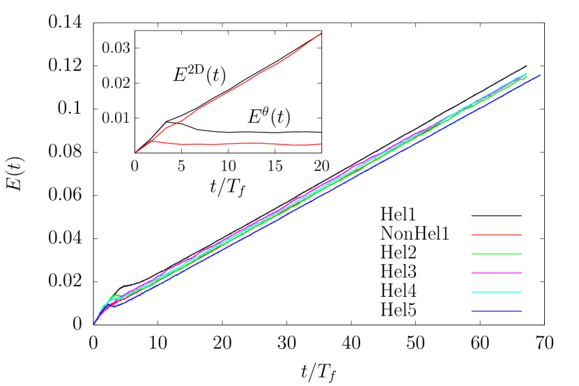
Figure 1: Time evolution of the total energy for datasets with either fully helical or nonhelical forcing. Inset: Time evolution of $E^{\theta}(t)$ and $E^{\rm 2D}(t)$ up to $t/T_{f}=20$ for one realisation of datasets (Hel1) and (NonHel1), respectively. The color scheme of the inset is the same as that of the main graph.

3 Numerical simulations

We study numerically the dynamics of incompressible 2D3C flows given by eqs. (1) subject to helical and nonhelical forcing in order to shed light on the effect of the forcing-induced correlation between $\theta$ and $\omega$ on the energy flux from small to large scales. Furthermore, we investigate the influence of forcing on a bandwidth on the scaling properties of $E^{\theta}(k)$. For this purpose, it is necessary to inject energy into the system at the small scales, to ensure large scale separation between the forcing scale and the largest resolved scale in order to study the inverse cascade, while still resolving small-scale dynamics. We consider the Navier-Stokes equations with the Laplace operator replaced by higher-order hyperviscous dissipation

$$\partial_{t}{\bm{u}}=-\nabla\cdot({\bm{u}}\otimes{\bm{u}})-\nabla P+\nu(-1)^{n+1}\Delta^{n}{\bm{u}}+{\bm{f}}\ ,$$ (12)

$$\nabla\cdot{\bm{u}}=0\ ,$$ (13)

where $n=4$. Equations (12)-(13) are solved numerically on a triply periodic domain $V=[0,2\pi]^{3}$ using a pseudospectral code with full dealiasing by truncation following the two-thirds rule. The forcing is given by a white-in-time random process in Fourier space

$$\langle\hat{\bm{f}}_{\bm{k}}(t)\hat{\bm{f}}^{*}_{\bm{q}}(t^{\prime})\rangle=F^{2}\delta_{{\bm{k}},{\bm{q}}}\delta(t-t^{\prime})\hat{Q}_{\bm{k}},$$ (14)

where $\hat{Q}_{\bm{k}}$ is a projector applied to guarantee incompressibility and $F$ is nonzero in a given band of Fourier modes concentrated at intermediate to small scales, see table 1 for details. Since the 2D component of u displays an inverse energy transfer and no large-scale energy removal is used, the simulations will reach a statistically stationary state only after very long evolution times. Here, we terminate the simulations before the formation of a condensate at the largest resolved scales. In order to obtain statistical measurements we therefore generate ensembles over independent runs. The simulations differ in the level of helicity injection, in the scale separation between the forcing scale and the largest resolved scale and in the width of the forcing band. Runs with fully helical forcing are labelled (Hel) followed by a number while those carried out with helically neutral forcing are labelled (NonHel) and those with fractionally helical forcing are labelled (FracHel). Further details on runtime, ensemble size, number of grid points, location of the forcing band, etc., are given in table 1.

In order to compare between different datasets, the parameters are chosen such that the growth rate of the total energy (per unit volume), $dE/dt$, remains the same between different datasets. The energy is given as

$$E(t)=\sum_{k\neq 0}E(k,t)\ ,$$ (15)

where $E(k,t)=E^{\rm 2D}(k,t)+E^{\theta}(k,t)$ is the total energy spectrum. The energy of the 2D-component, $E^{\rm 2D}(t)$, and that of the out-of-plane component, $E^{\theta}(t)$, are defined analogously. The time evolution of $E(t)$ for all datasets is shown in the main graph of Fig. 1. The time evolution of $E^{\rm 2D}(t)$ and $E^{\theta}(t)$ for dataset (Hel1) and dataset (NonHel1) is presented in the inset of Fig. 1, where one can see that the energy growth is due to the 2D component only, while the $\theta$-component reaches a statistically stationary state, with $E^{\theta}(t)$ being larger for dataset (Hel1) compared to dataset (NonHel1). We will come back to this point in section 3.2.

In what follows we distinguish between two main questions. Firstly, for helical forces we investigate the influence of extending the domain where the forcing is active from a single shell to a wider band of Fourier modes. Second, we compare the effect of helical and nonhelical forces both active in a wavenumber shell centered at $k_{f}$ in order to investigate the effect of forcing-induced correlation between $\theta$ and $\omega$ on the dynamics. The main observables will be energy fluxes and spectra.

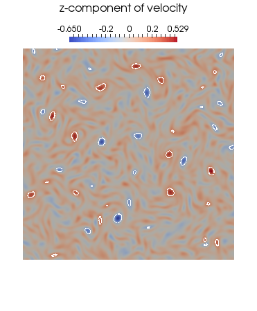
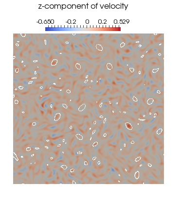
helical                                                                       nonhelical

Figure 2: Visualisations of $\theta$ snapshots for datasets (Hel1) (left) and (NonHel1) (right) at $t/T_{f}=25$, the white contour lines indicate the regions with vorticity $|\omega|=0.5$.

In order to clearly distinguish between the dynamics of helically and nonhelically forced 2D3C flows, we generated two ensembles of runs from random initial data with identical parameters concerning resolution, forcing band, forcing magnitude and run time. The two ensembles only differed with respect to the helicity of the forcing. In both cases the forcing is active on a single wavenumber shell. According to the discussion in section 2, it can be expected that $\theta$ and $\omega/k_{f}$ behave similarly for dataset (Hel1). In contrast, no connection between $\theta$ and $\omega/k_{f}$ is given through the equations of motion for dataset (NonHel1). Visualisations of $\theta$ compared with contour lines of $|\omega|$ are shown in Fig. 2 for single realisations taken from datasets (Hel1) (left panel) and (NonHel1) (right panel) at $t/T_{f}=25$. As can be seen from the figures, intense regions of $\theta$ indeed coincide clearly with intense regions of $|\omega|$ for dataset (Hel1), while no such effect can be identified for dataset (NonHel1). Visualisations of rapidly rotating flows subject to helical forcing show similar correlations between vorticity and the velocity component parallel to the rotation axis Mininni10b .

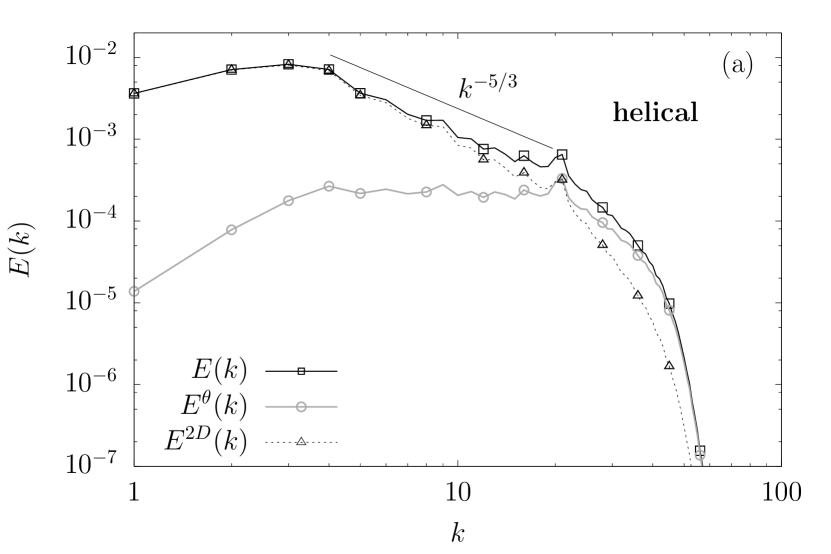
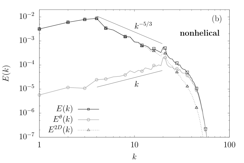
Figure 3: Energy spectra for (a) dataset (Hel1), and (b) dataset (NonHel1) at $t/T_{f}=25$.

Figure 4: Comparison between $E^{\theta}(k)$ and $(k^{2}/k_{f}^{2})E^{\rm 2D}(k)$ for the different datasets. Left: Single-shell forcing, datasets (Hel1), (Hel2), (Hel5) and (Hel6). Right: Band forcing, runs (Hel3), (Hel4) and (Hel7) with $k_{f}^{*}\simeq(k_{\rm min}+k_{\rm max})/2$. Data corresponds either to time-averages for runs (Hel2) and (Hel3), ensemble average at $t/T_{f}=84$ for (Hel1), ensemble average at $t/T_{f}=30$ for (Hel6) and (Hel7) or the last snapshot in the simulation for (Hel4) and (Hel5). Spectra corresponding to different datasets are shifted in order to facilitate the readability of the figure.

Figure 5: Comparison between $E^{\theta}(k)$ and $(k^{2}/k_{f}^{2})E^{\rm 2D}(k)$ from simulations forced with different fractions of helicity injection. The database analysed here consists of runs (Hel6), (FracHel1), (FracHel2) and (FracHel3) corresponding respectively to the value of $x=0,\,0.2,\,0.5$ and $1$. Data corresponds either to the ensemble average at $t/T_{f}=30$ for (Hel6) or to the last snapshot in the simulation for the remaining datasets. Spectra corresponding to different datasets are shifted in order to facilitate the readability of the figure.

Figure 6: Fluxes of $E^{\theta}(k)$ and $E^{\rm 2D}(k)$ at early times for datasets (Hel1) and (NonHel1): (a) $t/T_{f}=3.4$, (b) $t/T_{f}=8.4$.

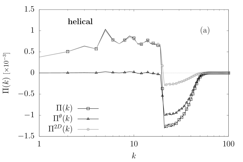
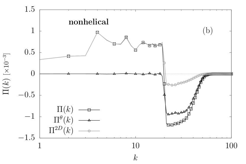
Figure 7: Energy fluxes for (a) dataset (Hel1), and (b) dataset (NonHel1) at $t/T_{f}=25$.

3.1 Spectral scaling

A further quantitative assessment of the correlation between $\theta$ and $\omega$ can be carried out through a comparison of the energy spectra. In particular, we consider the energy spectra of the full velocity field, of its $\theta$- and 2D-components. All three energy spectra obtained from datasets (Hel1) and (NonHel1) are shown in Fig. 3 at $t/T_{f}=25$. Two main phenomenological results can be obtained from this figure. Firstly, as expected, the 2D-component is unaffected by helicity of the forcing, as ${\bm{u}}^{\rm 2D}$ displays inverse-cascade spectra in both cases with a spectral index close to the predicted $-5/3$ for 2D turbulence Kraichnan67 . Furthermore, the 2D spectra are also qualitatively very similar in regions outwith the inertial range. Second, the $\theta$-component is clearly sensitive to the helicity of the forcing, as $E^{\theta}(k)$ shows the expected 2D absolute equilibrium scaling, $E^{\theta}(k)\sim k$, for $k<k_{f}$ in case of dataset (NonHel1), while no such scaling is observed for $E^{\theta}(k)$ for dataset (Hel1). Figure 4 provides a comparison between $E^{\theta}(k)$ and $(k/k_{f}^{*})^{2}E^{\rm 2D}(k)$ for single-shell and band forcing. The left panel presents the single-shell cases (Hel1), (Hel2) and (Hel5). It can clearly be seen that the scaling predicted by Eq. (11) is in agreement with the data for all $k$ except the smallest two wavenumbers, independent of the separation between the forcing shell and the smallest resolved wavenumber. Similar results are obtained for the band-forced case shown in the right panel for runs (Hel3) and (Hel4), provided $k_{f}$ is replaced by an ‘effective forcing wavenumber’ $k_{f}^{*}\simeq(k_{\rm min}+k_{\rm max})/2$ for a forcing band given by the interval $[k_{\rm min},k_{\rm max}]$. In summary, the scaling given by Eq. (11) for helical forcing also applies for the more general case of band forcing to a good approximation. For this reason we restrict our attention to single-shell forcing in the remainder of this paper, where we focus on the nonuniversal dynamics of $\theta$. In Fig. 5 the comparison between $E^{\theta}(k)$ and $(k/k^{*}_{f})^{2}E^{2D}(k)$ for fractionally helical forcing is presented. In this analysis we have used the following sets of simulations, (Hel6) $x=0$, (FracHel1) $x=0.2$, (FracHel2) $x=0.5$ and (FracHel3) $x=1$ at $2048^{2}$ collocation points. From Fig. 5 it is visible that upon decreasing the helicity injected by the forcing, hence upon decreasing the value of $x$, the two spectra tend to overlap perfectly following the prediction given in Eq. (11). Important deviations are already visible at values of $x$ around $0.5$ while for $x=1$ the scalar component is again completely passive as expected and it develops an absolute equilibrium spectrum at wavenumbers smaller than $k_{f}$. The results presented in Fig. 5 clearly show a non-universal nature of the passive component, which changes its behaviour depending on the helical properties of the external forcing.

3.2 Fluxes and nonuniversal dynamics

As discussed earlier, while ${\bm{u}}^{\rm 2D}$ undergoes an inverse energy cascade, $\theta$ appears to become statistically stationary after an initial transient in both cases (Hel1) and (NonHel1). In case (NonHel1), such observation is in agreement with the results on passive scalar advection in 2D turbulence, where $\theta$ cascades from large to small scales and attains equipartition at scales larger than the forcing scale. However, in case (Hel1) the out-of-plane component is active and forced in a finite band of Fourier modes (here, a single shell), which implies that the large-scale dynamics of $\theta$ is connected to the nonstationary inverse-cascade dynamics of ${\bm{u}}^{\rm 2D}$. In particular, $E^{\theta}(k,t)$ cannot be statistically stationary at $k<k_{f}$ according to Eq. (11), however, the scaling $E^{\theta}(k,t)\sim k^{1/3}$ results in $E^{\theta}(k,t)\to 0$ for $k\to 0$. The latter implies that the total energy of $\theta$ in the region $k\leqslant k_{f}$ is dominated by the contribution at the forcing shell

$$E^{\theta}(t)_{|k\leqslant k_{f}}\simeq\int_{k_{0}(t)}^{k_{f}}E^{\theta}(k,t)dk=k_{f}^{4/3}-k_{0}(t)^{4/3}\ ,$$ (16)

where $k_{0}(t)$ is the smallest wavenumber at which $\theta$ contains a significant amount of energy at time $t$. Since $k_{0}(t)\to 0$ for $t\to\infty$, $E^{\theta}(t)$ indeed tends to a constant for $t\to\infty$, even though $E^{\theta}(k,t)$ is not stationary according to eq. (11).

Figure 8: Homo- and heterochiral subfluxes at $t/T_{f}=25$. (a) $\Pi(k)$ (squares), $\Pi^{\rm HO}(k)$ (triangles) and $\Pi^{\rm HE}(k)$ for helical forcing. (b) The same for nonhelical forcing.

Figure 9: Homochiral subfluxes $\Pi^{\rm HO}_{+}(k)$ (circles) and $\Pi^{\rm HO}_{-}(k)$ (triangles) for (a) helical forcing (Hel1) and (b) nonhelical forcing (NonHel1) at $t/T_{f}=25$.

In order to understand the matter more clearly, it is instructive to consider the energy fluxes

$$\Pi(k) =-\sum_{k^{\prime}=1}^{k}\sum_{|{{\bm{k}}}|=k^{\prime}}\hat{\bm{u}}_{\bm{k}}\cdot\sum_{{\bm{k}}+{\bm{p}}+{\bm{q}}=0}(i{\bm{k}}\cdot\hat{\bm{u}}_{\bm{p}})\hat{\bm{u}}_{\bm{q}}\ ,$$ (17)

$$\Pi^{\theta}(k) =-\sum_{k^{\prime}=1}^{k}\sum_{|{{\bm{k}}}|=k^{\prime}}\hat{\theta}_{\bm{k}}\sum_{{\bm{k}}+{\bm{p}}+{\bm{q}}=0}(i{\bm{k}}\cdot\hat{\bm{u}}^{\rm 2D}_{\bm{p}})\hat{\theta}_{\bm{q}}\ ,$$ (18)

$$\Pi^{2D}(k) =-\sum_{k^{\prime}=1}^{k}\sum_{|{{\bm{k}}}|=k^{\prime}}\hat{\bm{u}}^{\rm 2D}_{\bm{k}}\cdot\sum_{{\bm{k}}+{\bm{p}}+{\bm{q}}=0}(i{\bm{k}}\cdot\hat{\bm{u}}^{\rm 2D}_{\bm{p}})\hat{\bm{u}}^{\rm 2D}_{\bm{q}}\ .$$ (19)

While $\Pi^{\theta}(k)$ must vanish in case (NonHel1) for $k<k_{f}$, the correlation between $\theta$ and $\omega$ in case (Hel1) should result in a subleading correction which vanishes in the limit $t\to\infty$. That is, $\Pi^{\theta}(k)$ should be nonzero during the transient stage for case (Hel1), i.e., before $\Pi^{\rm 2D}(k)=const$ for $k<k_{f}$ and $\Pi^{\theta}(k)=const$ for $k>k_{f}$ is established. The fluxes $\Pi^{\rm 2D}(k,t)$ and $\Pi^{\theta}(k,t)$ are shown in Fig. 6 for two times at $t/T_{f}=3.4$ and $t/T_{f}=8.4$. As can be seen, $\Pi^{\rm 2D}(k,t)$ is nearly identical at both times for (Hel1) and (NonHel1), while the two cases are distinct concerning the behaviour of $\Pi^{\theta}(k,t)$. In case (NonHel1), only a direct transfer of $E^{\theta}(k)$ with a well-established forward flux is present at $t/T_{f}=3.4$. In particular, there is no inverse $E^{\theta}(k)$-flux. In contrast, for case (Hel1), $\Pi^{\theta}(k,t)$ is depleted in the direct transfer region $k>k_{f}$ with nonzero inverse $E^{\theta}(k)$-flux, which decreases with time as can be seen by comparing Figs. 6(a) and (b). Figure 7 presents the fluxes $\Pi(k)$, $\Pi^{\theta}(k)$ and $\Pi^{\rm 2D}(k)$ at $t/T_{f}=25$, where $E^{\theta}(t)$ is statistically stationary. In the region $k<k_{f}$ we indeed find $\Pi^{\theta}(k)=0$ in both cases, while the entire inverse energy flux is carried by the 2D component. As can be seen from the figure, the fluxes $\Pi^{\theta}(k)$ and $\Pi^{\rm 2D}(k)$ are now very similar for the two datasets. The absolute equilibrium spectral scaling of $E^{\theta}(k)$ is in accord with $\Pi^{\theta}(k)=0$ in the region $k<k_{f}$ for case (NonHel1), while for the helically forced case $\theta(k)$ is out of equilibrium. In summary, under helical forcing the out-of-plane component $\theta$ develops a transient inverse transfer, which is absent in case (NonHel1).

The differences we find in the behaviour of $\theta$ must be caused by a superabundance of helical velocity field modes of one sign close to the forcing shell. Furthermore, it is known that helicity cannot play a role in the 2D-dynamics, that is, any interaction of helical modes should participate democratically in the inverse energy cascade of ${\bm{u}}^{\rm 2D}$. In this context, it is important to note that the transient inverse energy flux of $\theta$ is a three-dimensional effect which is intrinsically connected to the breaking of mirror symmetry by strongly helical forcing. In fact, a fully 3D inverse cascade can be achieved by breaking mirror symmetry at all scales through projection onto one helical component Biferale12 ; Biferale13a , and interactions of helical modes of the same sign also contribute to a subleading 3D inverse energy transfer in full Navier-Stokes dynamics Alexakis17 . Here, we only project the Fourier components of the force onto the positively helical sector letting the nonlinear interactions generate velocity field modes of either sign of helicity. This leads to a dominance of positively helical modes in the presence of a strong 2D inverse transfer. It is therefore of interest to establish which interactions of helical modes are now mediating the inverse energy transfer.

We first define the energy subfluxes which correspond to helical interactions involving only velocity modes of a fixed sign of helicity

$$\Pi^{\rm HO}_{+}(k) =-\sum_{k^{\prime}=1}^{k}\sum_{|{{\bm{k}}}|=k^{\prime}}\hat{\bm{u}}^{+}_{\bm{k}}\cdot\sum_{{\bm{k}}+{\bm{p}}+{\bm{q}}=0}(i{\bm{k}}\cdot\hat{\bm{u}}^{+}_{\bm{p}})\hat{\bm{u}}^{+}_{\bm{q}}\ ,$$ (20)

$$\Pi^{\rm HO}_{-}(k) =-\sum_{k^{\prime}=1}^{k}\sum_{|{{\bm{k}}}|=k^{\prime}}\hat{\bm{u}}^{-}_{\bm{k}}\cdot\sum_{{\bm{k}}+{\bm{p}}+{\bm{q}}=0}(i{\bm{k}}\cdot\hat{\bm{u}}^{-}_{\bm{p}})\hat{\bm{u}}^{-}_{\bm{q}}\ ,$$ (21)

where the label HO stands for homochiral. As mentioned above, $\Pi^{\rm HO}_{+}(k)$ and $\Pi^{\rm HO}_{-}(k)$ contribute to a subleading inverse energy transfer even in 3D. Their combined contribution is the total homochiral flux Biferale17 ; Alexakis17

$$\Pi^{\rm HO}(k)=\Pi^{\rm HO}_{+}(k)+\Pi^{\rm HO}_{-}(k)\ ,$$ (22)

while interactions involving velocity modes of oppositely-signed helicity are combined to define the heterochiral flux Biferale17 ; Alexakis17

$$\Pi^{\rm HE}(k)=\Pi(k)-\Pi^{\rm HO}(k)\ .$$ (23)

Fully helical forcing leads to an imbalance between homo- and heterochiral energy fluxes as shown in Fig. 8. For the case (Hel1) we can see that close to the energy injection scale, where the dynamics is dominated by Fourier modes of positive helicity, $\Pi(k)$ is mainly given by $\Pi^{\rm HO}(k)$ with $\Pi^{\rm HE}(k)$ being negligible, see Fig. 8(a). For the case (NonHel1) the two contributions are almost identical, as it should be for a 2D simulation where helicity does not play any role, see Fig. 8(b). Owing to the positively helical forcing, in case (Hel1) the homochiral flux can be expected to be mostly given by its component consisting of positively helical modes, i.e. $\Pi^{\rm HO}_{+}(k)$. This is indeed the case as can be seen in Fig. 9(a), which presents a comparison between $\Pi^{\rm HO}_{+}(k)$ and $\Pi^{\rm HO}_{-}(k)$ for case (Hel1). Fig. 9(b) instead shows that $\Pi^{\rm HO}_{+}(k)$ and $\Pi^{\rm HO}_{-}(k)$ are the same in case (NonHel1).

4 Conclusions

It is known that a sustained 3D inverse energy cascade can be achieved by projecting the Navier-Stokes equations onto one helical subspace (homochiral turbulence) Biferale12 ; Biferale13a ; Waleffe92 . In a homochiral 2D3C flow, the 2D vorticity would be fully correlated with the out-of-plane component at all times. As a result, the out-of-plane component is not passive anymore and develops an inverse cascade similarly to what the 2D velocity field does Biferale17 . Although interesting from a theoretical point of view, such a system is somewhat artificial because the projection operation must be carried out dynamically in order to remove modes of opposite helicity which are generated by nonlinear interactions. The latter implies that a system described by the helically projected Navier-Stokes equations can be studied numerically only. Here, we present the application of helical forcing as a way of making the out-of-plane component active while maintaining the full 2D3C Navier-Stokes equations. As such, it is potentially realizable also in a laboratory. We show that even in this most realistic case the turbulent transfer for the out-of-plane component can be changed through an appropriate forcing, with a sign reversal in the direction of the energy cascade in the presence of a strong helical stirring mechanism. Also here, nonzero helicity input results in a correlation of the vorticity of the 2D-velocity field with the third component. Such correlation implies that the out-of-plane component can be thought as an active scalar advected by the 2D velocity field.

The correlation between the 2D vorticity and the third component leads to a nonequilibrium large-scale dynamics which is reflected in the scaling of its energy spectrum. While the energy spectrum of one uncorrelated passive scalar would display absolute equilibrium scaling, that of the correlated out-of-plane component does not. Moreover, we show that the correlation induces a transient inverse energy transfer which is mediated by homochiral interactions. In other words, a helical input in a 2D3C flow results in a transient 3D contribution to the inverse energy transfer, which would be, otherwise, a purely 2D effect in case of no helicity input. A similar effect should be present in helically forced flows under rapid rotation and in conducting flows in the presence of a strong mean magnetic field Alexakis11 ; buzzicotti2017energy .

Our study provides further evidence that scalar quantities transported by a velocity field might develop non-universal transfer properties in the presence of a correlation among the injection and the advecting velocity. Similar effects exist for 2D MHD, where the magnetic potential performs an inverse cascade while a passive scalar develops a forward transfer. Furthermore, for surface quasi-geostrophic flows, although both the potential temperature and a passive dye would perform a direct cascade, they have different scaling laws already at the level of low-order statistical objects. These significant differences are due to the correlations between the active scalar input and the advected velocity, as can be seen also by studying the evolution of Lagrangian trajectories of the two active and passive fields celani2004active .

Acknowlegdements

We acknowledge useful discussions with A. Alexakis and R. Benzi. The research leading to these results has received funding from the European Union’s Seventh Framework Programme (FP7/2007-2013) under grant agreement No. 339032 and from the COST Action Programme.

Authors contribution statement

All the authors were involved in the preparation of the manuscript. All the authors have read and approved the final manuscript.

References

- [1] C. Cambon and L. Jacquin. Spectral approach to non-isotropic turbulence subjected to rotation. J. Fluid Mech., 202:295–317, 1989.
- [2] F. Waleffe. Inertial transfers in the helical decomposition. Phys. Fluids A, 5:677–685, 1993.
- [3] L. M. Smith and F. Waleffe. Transfer of energy to two-dimensional large scales in forced, rotating three-dimensional turbulence. Phys. Fluids, 11:1608, 1999.
- [4] Q. Chen, S. Chen, G. L. Eyink, and D. D. Holm. Resonant interactions in rotating homogeneous three-dimensional turbulence. J. Fluid Mech., 542:139–164, 2005.
- [5] P. D. Mininni, A. Alexakis, and A. Pouquet. Scale interactions and scaling laws in rotating flows at moderate Rossby numbers and large Reynolds numbers. Phys. Fluids, 21:015108, 2009.
- [6] B. Gallet. Exact two-dimensionalization of rapidly rotating large-Reynolds-number flows. J. Fluid Mech., 783:412–447, 2015.
- [7] A. Alexakis. Rotating Taylor-Green flow. J. Fluid Mech., 769:46–78, 2015.
- [8] L. Biferale, F. Bonaccorso, I. M. Mazzitelli, M. A. T. van Hinsberg, A. S. Lanotte, S. Musacchio, P. Perlekar, and F. Toschi. Coherent Structures and Extreme Events in Rotating Multiphase Turbulent Flows. Phys. Rev. X, 6:041036, 2016.
- [9] Sébastien Galtier. Theory for helical turbulence under fast rotation. Physical Review E, 89(4):041001, 2014.
- [10] H. K. Moffatt. On the suppression of turbulence by a uniform magnetic field. J. Fluid Mech., 28:571–592, 1967.
- [11] A. Alemany, R. Moreau, P. L. Sulem, and U. Frisch. Influence of external magnetic field on homogeneous MHD turbulence. J. Méc., 18:280–313, 1979.
- [12] O. Zikanov and A. Thess. Direct numerical simulation of forced mhd turbulence at low magnetic reynolds number. J. Fluid Mech., 358:299 333, 1998.
- [13] B. Gallet and C. R. Doering. Exact two-dimensionalization of low-magnetic-Reynolds-number flows subject to a strong magnetic field. J. Fluid Mech., 773:154–177, 2015.
- [14] Alexandros Alexakis. Two-dimensional behavior of three-dimensional magnetohydrodynamic flow with a strong guiding field. Phys. Rev. E, 84:056330, 2011.
- [15] Barbara Bigot and Sébastien Galtier. Two-dimensional state in driven magnetohydrodynamic turbulence. Phys. Rev. E, 83:026405, 2011.
- [16] Leslie M Smith and Fabian Waleffe. Transfer of energy to two-dimensional large scales in forced, rotating three-dimensional turbulence. Physics of fluids, 11(6):1608–1622, 1999.
- [17] G. Falkovich, K. Gawȩdzki, and M. Vergassola. Particles and fields in fluid turbulence. Rev. Mod. Phys., 73:913–975, 2001.
- [18] L. Biferale, M. Buzzicotti, and M. Linkmann. From two-dimensional to three-dimensional turbulence through two-dimensional three-component flows. Phys. Fluids, 29:111101, 2017.
- [19] H. K. Moffatt. Note on the triad interactions of homogeneous turbulence. J. Fluid Mech., 741:R3, 2014.
- [20] P. D. Mininni and A. Pouquet. Helicity cascades in rotating turbulence. Phy. Rev. E, 79:026304, 2009.
- [21] T. Teitelbaum and P. D. Mininni. Effect of helicity and rotation on the free decay of turbulent flows. Physical review letters, 103:014501, 2009.
- [22] P. D. Mininni and A. Pouquet. Rotating helical turbulence. i. global evolution and spectral behavior. Phys. Fluids, 22:035105, 2010.
- [23] P. D. Mininni and A. Pouquet. Rotating helical turbulence. ii. intermittency, scale invariance, and structures. Phys. Fluids, 22:035106, 2010.
- [24] V. Dallas and S. M. Tobias. Forcing-dependent dynamics and emergence of helicity in rotating turbulence. J. Fluid Mech., 798:682–695, 2016.
- [25] L. Biferale, S. Musacchio, and F. Toschi. Inverse energy cascade in three-dimensional isotropic turbulence. Phys. Rev. Lett., 108:164501, 2012.
- [26] L. Biferale, S. Musacchio, and F. Toschi. Split Energy-Helicity cascades in three dimensional Homogeneous and Isotropic Turbulence. J. Fluid Mech., 730:309–327, 2013.
- [27] P. Constantin and A. Majda. The Beltrami spectrum for incompressible flows. Commun. Math. Phys., 115:435–456, 1988.
- [28] F. Waleffe. The nature of triad interactions in homogeneous turbulence. Phys. Fluids A, 4:350–363, 1992.
- [29] Antonio Celani, Massimo Cencini, Andrea Mazzino, and Massimo Vergassola. Active and passive fields face to face. New Journal of Physics, 6(1):72, 2004.
- [30] R. H. Kraichnan. Inertial ranges in two-dimensional turbulence. Phys. Fluids, 10(10):1417, 1967.
- [31] D. K. Lilly. Numerical simulation of two-dimensional turbulence. Phys. Fluids, 12:II–240–II–249, 1969.
- [32] J. Sommeria. Experimental study of the two-dimensional inverse energy cascade in a square box. J. Fluid Mech., 170:139–168, 1986.
- [33] T. Gotoh. Energy spectrum in the inertial and dissipation ranges of two-dimensional steady turbulence. Phys. Rev. E, 57:2984–2991, 1998.
- [34] J. Paret and P. Tabeling. Intermittency in the two-dimensional inverse cascade of energy: experimental observations. Phys. Fluids, 10:3126–3136, 1998.
- [35] G. Boffetta and R. E. Ecke. Two-dimensional turbulence. Annu. Rev. Fluid Mech., 44:427–451, 2012.
- [36] Alexandros Alexakis. Helically decomposed turbulence. Journal of Fluid Mechanics, 812:752–770, 2017.
- [37] Michele Buzzicotti, Hussein Aluie, Luca Biferale, and Moritz Linkmann. Energy transfer in turbulence under rotation. arXiv preprint arXiv:1711.07054, 2017.