Software paper for submission to the Journal of Open Research Software

 

(1) Overview

Title

Magpy: A C++ accelerated Python package for simulating magnetic nanoparticle stochastic dynamics

Paper Authors

1. Laslett, Oliver
2. Waters, Jonathon
3. Fangohr, Hans
4. Hovorka, Ondrej

Paper Author Roles and Affiliations

1. Engineering and the Environment, University of Southampton, Southampton, SO17 1BJ, UK.
2. Engineering and the Environment, University of Southampton, Southampton, SO17 1BJ, UK.
3. Engineering and the Environment, University of Southampton, Southampton, SO17 1BJ, UK. European XFEL GmbH, Holzkoppel 4, 22869 Schenefeld, Germany
4. Engineering and the Environment, University of Southampton, Southampton, SO17 1BJ, UK.

Abstract

Magpy is a C++ accelerated Python package for modelling and simulating the magnetic dynamics of nano-sized particles. Nanoparticles are modelled as a system of three-dimensional macrospins and simulated with a set of coupled stochastic differential equations (the Landau-Lifshitz-Gilbert equation), which are solved numerically using explicit or implicit methods. The results of the simulations may be used to compute equilibrium states, the dynamic response to external magnetic fields, and heat dissipation. Magpy is built on a C++ library, which is optimised for serial execution, and exposed through a Python interface utilising an embarrassingly parallel strategy. Magpy is free, open-source, and available on github under the 3-Clause BSD License.

Keywords

magnetism; macrospin; nanoparticles; physics; biomedicine; nanomedicine; stochastic; dynamics; numerical methods; Python; C++

Introduction

Magpy is an open-source C++ and Python package that models nanoparticles and simulates their magnetic state over time. The magnetic dynamics of atoms within materials are described by the Landau-Lifshitz-Gilbert (LLG) equation [1], which is a nonlinear stochastic differential equation (SDE). The best choice of numerical method to solve the LLG dynamics is an open research question. Therefore, the numerical solvers in Magpy are implemented in a generic form, independent from the equations of magnetism, which allows the methods to be tuned or replaced easily. The current implementation includes the widely used Heun scheme [2] and the first open-source implementation of the Milstein derivative-free fully implicit scheme [3]. Magpy also includes a rare-events model, valid under additional simplifying assumptions (detailed below), which avoids solving the LLG equation and consequently simulates single nanoparticles with significantly less computational effort.

The dynamics of magnetic nanoparticles play a crucial role in a number of emerging medical technologies. For example, magnetic particles have been used to enhance MRI images [4], deliver drugs inside the body [5], and destroy tumours by means of heat destruction [6]. The particles that enable these technologies are simulated computationally to augment traditional experiments and explore the effects of changing material properties. Although Magpy was designed with medical applications in mind, the software may be used to explain or predict the outcome of magnetic nanoparticle experiments in general.

A model for magnetic nanoparticle dynamics

Figure 1 shows a diagram of a magnetic nanoparticle, which comprises a large number of individual atoms arranged in a regular crystal lattice, each of which possesses a magnetic moment represented by a 3-dimensional vector. The net magnetisation of a material is simply the sum of the individual magnetic moments. For example, if the atoms are randomly oriented, the material has zero magnetisation; if they are all aligned, the material has a large magnetisation component. Atomic magnetic moments prefer to align with one another due to an exchange interaction force. This force is strong enough that, in nanoparticles that are particularly small ($<25$nm in diameter), the individual moments are approximately aligned and rotate coherently. Magpy uses this approximation to model the state of a particles’ atoms by a single 3-dimensional vector termed a macrospin, rather than simulate each atom individually. Magpy is able to simulate much longer timescales for the same computational effort compared to simulating the individual atoms due the greatly reduced degrees of freedom.

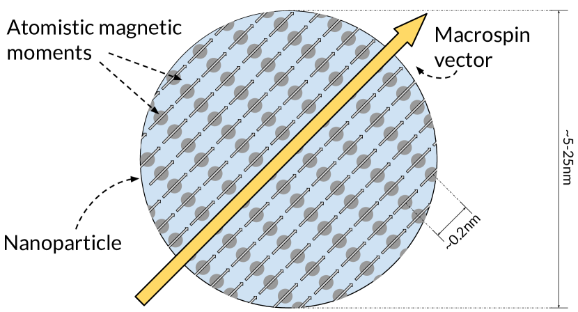
Figure 1: A two-dimensional sketch of a nanoparticle. The atoms of a magnetic material are packed into a regular crystal lattice and each is modelled by a three-dimensional magnetic moment that varies with time. Due to strong interactions between these magnetic moments in small particles, Magpy assumes they rotate coherently and are represented by a single macrospin vector.

The dynamics of a macrospin are described by the Landau-Lifshitz-Gilbert equation (LLG). For a detailed explanation of the origins and derivation of the LLG see [1]. The LLG is implemented in Magpy in a normalised form by replacing time with a reduced time variable $\ell$ (defined below), which ensures that the variables in the equation are around an order of magnitude of unity:

$$\derivative{\mathbf{m}_{k}}{\ell}=-\left(\mathbf{m}_{k}\times\left(\mathbf{h}_{k}+\bm{\xi}_{k}\right)\right)-\alpha\mathbf{m}_{k}\times\left(\mathbf{m}_{k}\times\left(\mathbf{h}_{k}+\bm{\xi}_{k}\right)\right)$$ (1)

where $\mathbf{m}_{k}\in\mathbb{R}^{3}$ is the unit vector of the $k^{\mathrm{th}}$ particle macrospin, $\alpha$ is a damping constant, $\bm{\xi}_{k}\in\mathbb{R}^{3}$ is a random term that models the thermal fluctuations experienced by the particle, and $\mathbf{h}_{k}$ is the effective magnetic field experienced by the particle. The effective field $\mathbf{h}_{i}$ comprises three different components [7], which are depicted in Figure 2 and given mathematically as:

$$\begin{split}\mathbf{h}_{i}=&-k_{i}\left(\mathbf{m}_{i}\cdot\mathbf{k}_{i}\right)\mathbf{k}_{i}-\mathbf{h}_{\mathrm{app}}\\ &-\sum_{j\neq i}\frac{\mu_{0}M_{\mathrm{s}}^{2}}{2\bar{K}}\frac{v_{j}}{4\pi\left|\mathbf{r}_{ij}\right|^{3}}\left(3\left(\mathbf{m}_{j}\cdot\mathbf{r}_{ij}\right)\mathbf{r}_{ij}-\mathbf{m}_{j}\right)\end{split}$$ (2)

The first term describes preferential alignment of $\mathbf{m}$ with the particle’s anisotropy axis, which acts in the unit direction $\mathbf{k}_{i}\in\mathbb{R}^{3}$ with magnitude $k_{i}$ (units Jm^-3). The second term describes the effect of an externally applied field $\mathbf{h}_{\mathrm{app}}\in\mathbb{R}^{3}$. The final term describes the field experienced by particle $i$ through a long-range dipole-dipole interaction with a nearby particle $j$, where $V_{j}$ is the volume (units m³) of particle $j$ and $v_{j}=V_{j}/\bar{V}$ is the reduced volume; $\bar{V}=1/N\sum_{n=0}^{N}V_{n}$ is the mean volume of all particles in the system; $\bar{K}=1/N\sum_{n=0}^{N}k_{n}$ is the mean anisotropy magnitude; $\mu_{0}=4\pi\times 10^{-7}$ is a constant (units mkgs^-2A^-2); $M_{\mathrm{s}}$ is the magnitude of the macrospin (the saturation magnetisation, units Am^-1) and $\mathbf{r}_{ij}\in\mathbb{R}^{3}$ and $r_{ij}$ are the unit vector and magnitude respectively of the reduced distance between particles $i$ and $j$. The reduced distance is the true distance (units m) divided by $\sqrt[3]{\bar{V}}$ and appears in equation (2) because the numerator and denominator of the interaction term are divided by $\bar{V}$, which has the effect of scaling both values close to unity. The prefactor $\mu_{0}M_{\mathrm{s}}^{2}/\quantity(2\bar{K})$ can be computed in advance and will also evaluate close to unity.

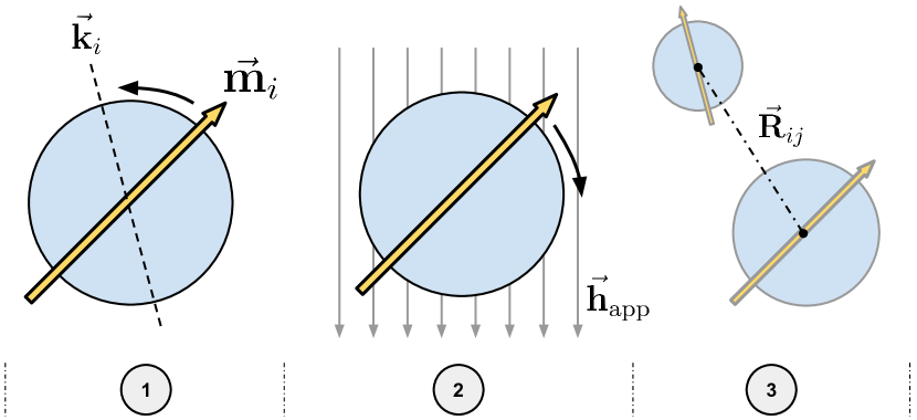
Figure 2: The three effective field contributions acting upon macrospin $i$. (1) The macrospin experiences a force towards alignment with the particle anisotropy axis (dashed line) $\mathbf{k}_{i}$ in either direction. (2) The macrospin is also forced towards aligning with the externally applied field direction (solid arrows) $\mathbf{h}_{\textrm{app}}$. (3) Finally, each macrospin is repelled and attracted by nearby macrospins. The force of the dipole-dipole interaction diminishes with distance (dash-dotted line) between two particles $\mathbf{R}_{ij}$.

The reduced simulation time is related to real time through:

$$\ell=t\frac{2\gamma\bar{K}}{M_{\mathrm{s}}\quantity(1+\alpha^{2})}$$ (3)

where $\gamma=1.76086\times 10^{11}$ is a constant (units rads^-1T^-1). The fluctuating thermal field is a vector of independent and identically normally distributed random variables ($\xi_{k}^{i}\quantity(\ell)$ is the $i^{th}$ component of the thermal field acting on macrospin $k$ at time $\ell$) such that the covariance between two components is [2]:

$$\left<\xi^{i}_{k}\left(\ell\right)\xi^{j}_{k}\left(\ell^{\prime}\right)\right>=\delta_{ij}\delta\left(\ell-\ell^{\prime}\right)\sqrt{\frac{\alpha k_{B}T}{\bar{K}V_{k}\quantity(1+\alpha^{2})}}$$ (4)

where $\delta_{ij}$ and $\delta\quantity(\ell-\ell^{\prime})$ are the Kronecker delta and Dirac delta functions respectively, $k_{B}$ is the Boltzmann constant (units m²kgs^-2K^-1) and $T$ is the temperature (units K).

Equations (1)-(4) describe the Magpy model of a system of magnetic nanoparticles. The equations are solved numerically at discrete time steps, resulting in a simulated trajectory of the system’s magnetic state. The simulation outputs, at each discrete time, the value of the applied magnetic field and the $x,y,z$ components of the magnetic state of every particle in the system. These results may be used to obtain the total magnetisation of the system $M\quantity(t)=M_{\mathrm{s}}\sum_{i}m_{i}\quantity(t)$, the average magnetisation of an ensemble of systems, static and dynamic hysteresis loops, and the energy dissipated by the system.

Multiple simulations with different random seeds but with identical initial conditions will result in different solutions due to the stochastic nature of the thermal field. For example Figure 3, shows the results of five simulations of a 3-particle chain from the same initial condition. The Magpy script used to generate the results is shown in Listing 4. In addition to individual trajectories, the expected system trajectory and higher order statistical moments may be obtained by sampling a multitude of individual simulations (the Monte-Carlo technique). The number of simulations required to obtain reasonable estimates of these statistical variables is large and depends on the system of interest.

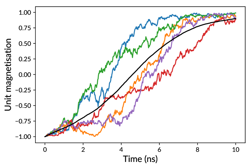
Figure 3: Simulating a chain of three particles (created in Magpy using Listing 4). (left) A chain structure of three identical particles are initialised with an external field applied along their anisotropy axis and their magnetisation initially against the applied field. (right) The coloured lines show the total magnetisation in the direction of the applied field for 5 simulations from the same initial condition (see left). The black line is the result of averaging 500 simulations from the same initial condition (i.e. the expected or mean trajectory).

⬇

import magpy as mp

\parchain3_model = mp.Model(

radius=[8e-9, 8e-9, 8e-9],

anisotropy=[4e3, 4e3, 4e3],

anisotropy_axis=[

[0., 0., 1.], [0., 0., 1.], [0., 0., 1.]],

magnetisation_direction=[

[0., 0., -1], [0., 0., -1], [0., 0., -1]],

location=[

[0., 0., -20e-9], [0., 0., 0.], [0., 0., 20e-9]],

magnetisation=400e3,

damping=0.1,

temperature=300.,

field_shape=’constant’,

field_amplitude=30e3)

\parchain3_ensemble = mp.EnsembleModel(base_model=chain3_model, N=500)

results = ensemble.simulate(

time_step=1e-13, end_time=1e-8, max_samples=500, n_jobs=4)

\partime = results.time

first_run_magnetisation = results.results[0].magnetisation()

ensemble_magnetisation = results.ensemble_magnetisation()

Figure 4: Simulating an ensemble of five hundred three-particle chains in Magpy (results shown in Figure 3). The three-particle chain model is instantiated (lines 3-16) using the Model object, which is defined by the properties and locations of each particle in the chain and the applied field. An ensemble of models is created using the EnsembleModel object (line 18), which simply represents a collection of individual models and is provided for convenience. The five hundred models are individually simulated (lines 19-20) and the computational work is distributed across four processes by setting n_jobs=4. The resulting magnetisation is computed for an individual model (line 23) and the entire ensemble of models (line 24).

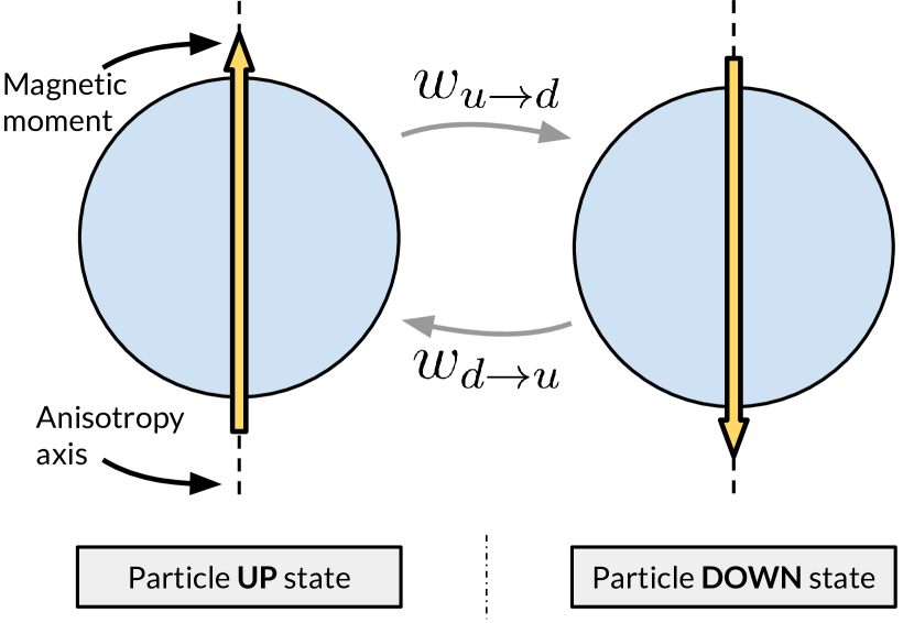
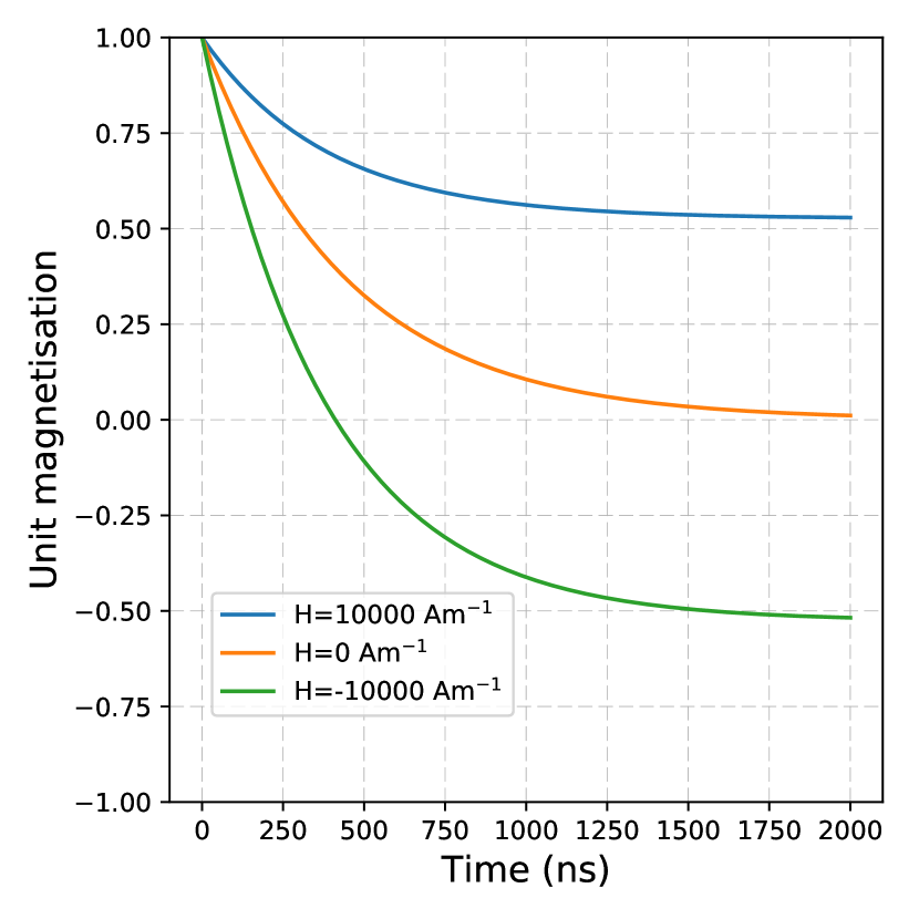
Figure 5: In the rare-events model, a single nanoparticle may occupy one of only two states: up or down, which each correspond to local energy minima around the anisotropy axis (left). The dynamics of the system are described by a master equation with transition rates $w_{u\to d/d\to u}$ between the two states. The solution of the master equation depends on the initial condition, particle properties and applied field. In this example (right) the particle is initialised up with probability 1 and allowed to relax into equilibrium (see Listing 6 for Magpy script). The equilibrium magnetisation depends upon the strength of the constant applied magnetic field.

⬇

import magpy as mp

\parHs = [100e2, 0.0, -100e2]

models = [

mp.DOModel(

radius=5e-9, anisotropy=5e4, damping=0.01,

magnetisation=400e3, temperature=300,

initial_probabilities=[1.0, 0.0], field_amplitude=H)

for H in Hs

]

results = [

model.simulate(end_time=2e-6, time_step=1e-10, max_samples=1000)

for model in models

]

expected_magnetisations = [res.magnetisation() for res in results]

Figure 6: Simulating three rare-events models with different applied field properties with Magpy (results plotted in Figure 5). The DOModel object, representing the rare-events model, is defined (lines 3-6) by the particle and applied field properties. Three identical particles are modelled each with a different value of the constant applied field amplitude (line 1). Each of the models is simulated (lines 9-12) and the expected magnetisation of each model is computed (line 13).

Simulating rare-events for single particles

Magpy provides an alternative, simpler model for simulating non-interacting, anisotropy-dominated particles. A particle is considered anisotropy-dominated if the effective field resulting from anisotropy $k$ is much greater than the thermal fluctuations and the externally applied field such that $\sigma\quantity(1-h)^{2}\gg 1$ (where $\sigma=KV/\quantity(k_{B}T)$ is termed the reduced energy barrier height). In these particles, the macrospin remains aligned with one direction of the anisotropy axis and exhibits long periods of negligibly small fluctuations around the axis separated by rare-events in which the macrospin reverses direction. Magpy approximates these dynamics as a jump process between two discrete states (up and down), which is described mathematically by the master equation:

$$\derivative{t}\matrixquantity[p_{\mathrm{u}}\quantity(t)\\ p_{\mathrm{d}}\quantity(t)]=\matrixquantity[-w_{\mathrm{u}\to\mathrm{d}}\quantity(t)&w_{\mathrm{d}\to\mathrm{u}}\quantity(t)\\ w_{\mathrm{u}\to\mathrm{d}}\quantity(t)&-w_{\mathrm{d}\to\mathrm{u}}\quantity(t)]\matrixquantity[p_{\mathrm{u}}\quantity(t)\\ p_{\mathrm{d}}\quantity(t)]$$ (5)

where the elements of $\mathbf{p}\quantity(t)=\matrixquantity[p_{\mathrm{u}}\quantity(t),p_{\mathrm{d}}\quantity(t)]^{T}$ are the probability that the system is in the up and down state respectively and $w_{\mathrm{u}\to\mathrm{d}}\quantity(t),w_{\mathrm{d}\to\mathrm{u}}\quantity(t)$ are the transition rates (units $s^{-1}$) between the two states. Note that the solution of the master equation is the time-evolution of the probability mass function over the discrete state space, whereas the solution of the Landau-Lifshitz-Gilbert equation is the time-evolution of a single random trajectory through the state-space $\mathbb{R}^{3}$.

The transition rates are computed in Magpy from the Néel-Brown model, which assumes that the field is applied parallel to the anisotropy axis direction [8]:

$$w_{\mathrm{u}\to\mathrm{d}/\mathrm{d}\to\mathrm{u}}\quantity(t)=\frac{2\gamma\alpha k_{B}T\sigma^{1.5}\quantity(1-h^{2}\quantity(t))}{VM_{\mathrm{s}}\sqrt{\pi}\quantity(1+\alpha^{2})}\quantity(1\pm h\quantity(t))e^{-\sigma\quantity(1\pm h\quantity(t))^{2}}$$ (6)

where $h\quantity(t)$ is the reduced applied field magnitude at time $t$ along the anisotropy direction. Equations (5) and (6) are solved numerically from an initial condition $\mathbf{p}\quantity(t_{0})=\matrixquantity[p_{\mathrm{u}}\quantity(t_{0}),p_{\mathrm{d}}\quantity(t_{0})]^{T}$ at time $t_{0}$ using an adaptive step Runge-Kutta solver (RK45) with Cash-Karp parameters [9]. The total magnetisation at time $t$ for a large ensemble of particles is computed as $M\quantity(t)=M_{\mathrm{s}}\quantity[p_{\mathrm{u}}\quantity(t)-p_{\mathrm{d}}\quantity(t)]$.

Figure 5 shows an example of a single particle simulated using the Magpy script in Listing 6, with a constant field applied along its anisotropy axis. The initial condition of the system is $\mathbf{p}\quantity(t_{0})=\matrixquantity[1,0]^{T}$ and the master equation is solved numerically. As time evolves, the probability that the particle flips into the down state $p_{\mathrm{d}}\quantity(t)$ increases and the expected magnetisation reduces. Eventually, the system reaches an equilibrium: in zero field the two states are equally likely and the system has zero magnetisation; for finite applied fields the system favours one state over the other.

Alternative software

Vinamax[10], implemented in Golang and also motivated by the medical applications of nanoparticles, provides similar functionality to Magpy. A distinguishing feature of Vinamax is its use of a multipole-expansion algorithm, which greatly improves the speed of computing the dipole-dipole interaction forces for large systems. Magpy computes the interaction field between every pair of particles (equation (2)), an operation with complexity $\mathcal{O}\quantity(n^{2})$; the multipole expansion method uses an approximation, which results in complexity $\mathcal{O}\quantity(n\log n)$. Vinamax implements a broad range of solvers for the LLG dynamics but currently does not include the fully implicit method.

The purpose of Magpy is not to simulate magnetic systems for which the macrospin assumption is not justified, such as for larger particles that exhibit more than a single domain or systems for which surface-to-surface atomistic interactions are significant. In these cases, the magnetic moments of the individual atoms must be modelled. Vampire [11] is an open-source C++ alternative to Magpy for atomistic simulation. Vampire reduces the significant additional computational effort required for simulating individual atoms by leveraging general purpose graphical processing units (GPGPUs). Alternatively, if the effects of temperature can be ignored and the atomistic magnetic moments are closely aligned, the magnetisation of material can be represented as a continuous function resulting in a spatial-temporal partial differential equation. This technique, termed micromagnetics, is implemented in a range of popular open-source packages: MuMax3 [12], OOMMF [13], fidimag [14], nmag [15].

As discussed, Magpy includes implementations for several numerical methods to compute approximate solutions to stochastic differential equations. Currently, the authors are not aware of a reliable alternative in C++ or Python for the fully implicit method [3]. Though there are mature packages for the solution of ordinary differential equations (e.g. sundials [16]) there are few options for stochastic differential equations. The most mature, SDElab [17] implemented in Matlab, is no longer under development and requires proprietary software. A re-implementation of SDElab using the open-source julia language is currently under development.

Implementation and architecture

Magpy consists of two components. Firstly, a C++ library implements the core simulation code, which comprises the nanoparticle model and numerical solvers. The second component is a Python interface to the C++ library functionality with additional features for setting up simulations and analysing their results.

The dynamics (Landau-Lifshitz-Gilbert equation), rare-events model, numerical methods, and the effective field calculations are implemented in a C++ library. C++ was the preferred programming language for implementing the computationally-intensive simulation because of its relatively fast performance and opportunities for optimisation. The Magpy C++ library is optimised for serial execution; uses the BLAS and LAPACK libraries; manages memory manually to minimise allocations and deallocations; and may be compiled with proprietary Intel compilers for enhanced performance on Intel architectures. Furthermore, the C++-11 standard contains features that support a functional programming paradigm (such as closures and partial application), which were used extensively in Magpy to improve testability and modularity of code. The entry point to the Magpy library is through two top-level functions: simulation::full_dynamics for the full model and simulation::dom_ensemble_dynamics for the rare-events model. Magpy does not provide a graphical user interface, simulations must be invoked by the user in a C++ program or using the alternative Python interface.

It was the authors’ opinion that scripting in C++ was not sufficiently usable because of the low-level syntax and the requirement for compiling scripts, which adds complexity for users. Python, on the other hand, is high-level, interpreted, and has been gaining popularity in the computational science community for the design of user interfaces [18, 19, 20] and as an easy-to-learn tool [21]. Therefore, Python was chosen as the preferred language for scripting and implementing the auxiliary components of Magpy. The interface between Python and C++ was written using Cython [22], which allowed the C++ library functions to be wrapped as Python functions and exposed as a Python package, while retaining the performance benefits of C++. The Python package includes additional features for building models and plotting the simulation results.

The typical workflow for a Magpy experiment consists of running multiple simulations of the same model in order to generate a distribution of possible trajectories, as in Figure 3. This motivates an embarrassingly parallel strategy in which each simulation executes concurrently on a single process, since no communication is required between the independent runs. Parallelism is implemented in Python using joblib. A minimum example of how joblib is used to execute tasks in parallel is shown in Listing 7. In Magpy, the user creates an ensemble of models (the EnsembleModel object in Listing 4 lines 3-18) and begins the simulation (EnsembleModel.simulate lines 19-20) utilising the requested number of cores (n_jobs). For each model in the ensemble, Magpy creates a new independent python process containing a copy of the model object. Each process then simulates its respective model by calling functions in the C++ library with the model parameters. As many as n_jobs simulations may execute concurrently. Once each simulation finishes, the results are returned from the C++ library to the individual python process. Once all processes have completed, the results are gathered back into the python process with which the user was originally interacting. This architecture is displayed graphically in Figure 8.

⬇

from joblib import Parallel, delayed

import time

\pardef slow_double(x):

time.sleep(1) # 1 second sleep

y = 2*x

return y

\parxs = [2, 6, 12, 24, 40, 72, 126, 240]

\par# Serial computation takes approximately 8s

ys_serial = [slow_double(x) for x in xs]

print(ys_serial)

#> [4, 12, 24, 48, 80, 144, 252, 480]

\par# Embarrassingly parallel computation takes approximately 2s

ys_parallel = Parallel(n_jobs=4)(delayed(slow_double)(x) for x in xs)

print(ys_parallel)

#> [4, 12, 24, 48, 80, 144, 252, 480]

Figure 7: A minimal example of an embarrassingly parallel computation with joblib. The function slow_double (line 4) doubles a single number and takes approximately one second. The objective is to evaluate the function with eight different arguments (line 9). This is achieved in serial with a for loop (line 12) by evaluating the function for each argument in the list singly, taking approximately eight seconds. However, this problem is embarrassingly parallel because all evaluations of slow_double may occur concurrently since each function call only depends on its initial argument. Using joblib, the eight function calls are evaluated on four processes as shown (line 17) by setting n_jobs=4. Two evaluations are distributed to each of the four processes, which execute concurrently, taking approximately two seconds.

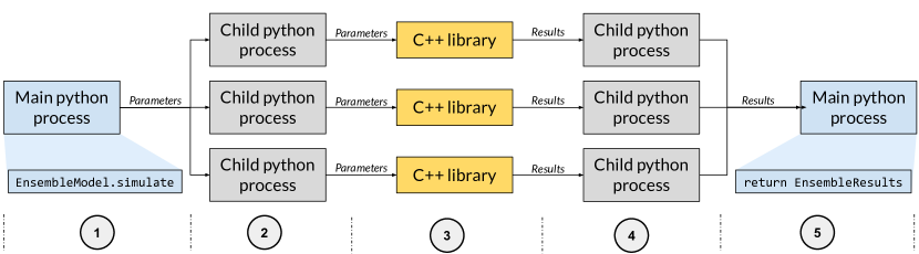
Figure 8: The flow of data through an ensemble simulation in Magpy. (1) The user instantiates an EnsembleModel object and calls the EnsembleModel.simulate function, specifying the number of CPU cores to utilise. (2) The main Python process spawns a new individual process for each model in the ensemble. (3) The individual processes each call the Magpy C++ library using their respective model parameters. (4) The results from the C++ simulation are returned to the individual python process. (5) When all the processes have finished, the results are collected on the main process to be analysed and plotted.

Quality control

Magpy has been tested to increase confidence in the correctness of the implementation, mathematics, and physics. The lowest level of tests, unit tests, assert that individual functions return the correct answer given a set of fixed arguments. The unit tests are designed to catch bugs during development and test the installation of the software. Continuous integration, using CircleCI, ensures that tests are automatically executed before changes are committed to the existing code repository on Github. The unit tests are implemented using GoogleTest for C++ functions and pytest for Python functions.

Numerical tests are necessary to confirm the stability and robustness of the numerical methods. Magpy includes scripts to evaluate the empirical convergence rates of the SDE solvers and compares them with analytic solutions [23, 3]. The numerical tests should be used during the development of new or existing solvers.

Finally, Magpy includes a series of Jupyter notebooks that present tutorials and examples, including comparisons of simulation results with theoretical solutions from alternative models in physics. These comparisons assert that the simulations, under the appropriate assumptions, correctly approximate the magnetic nanoparticle dynamics. The fundamental benefit of Jupyter notebooks is that they contain documentation, mathematics, figures, and executable code in a single format. However, this introduces additional maintenance, the example code in the notebooks must be updated when the interfaces or structure of the program changes. Therefore, we used the nbval tool as part of our testing practices to validate the consistency of the notebooks. The validation process asserts that the code examples run without error and that their result is consistent with the most recent documentation. Developers are expected to validate all existing notebooks before committing changes to the code base to ensure that they remain a relevant and executable form of documentation for users.

(2) Availability

Operating system

Available for all Linux based systems. Tested on Ubuntu 16.04 and RedHat 6.3.

Programming language

Python version 3.5 and a C++11/14 compatible compiler (e.g. G++-4.9 and above)

Additional system requirements

A single modern processor and 1GB of RAM is sufficient for basic models. 10MB of disk space is required for the Magpy source code, and a total of 35MB for the compiled libraries and interface.

Dependencies

g++-4.9, python3, openblas, setuptools, cython, numpy, matplotlib, toolz, joblib, scipy, transforms3d, pytest, nbval

List of contributors

Oliver W. Laslett, Jonathon Waters, Hans Fangohr, Ondrej Hovorka

Software location:

Archive

Name:

Zenodo

Persistent identifier:

10.5281/zenodo.1124942

Licence:

3-Clause BSD

Publisher:

Oliver Laslett

Version published:

1.1

Date published:

14/01/18

Code repository

Name:

Github

Persistent identifier:

https://github.com/owlas/magpy/tree/v1.1

Licence:

3-Clause BSD

Date published:

14/01/18

Language

English

(3) Reuse potential

Magpy was primarily designed for simulating the magnetic dynamics of nanosized particles. The simulation results may be used to compute heat dissipation, relaxation rates, and equilibrium states allowing the software to help predict, explain, or otherwise augment traditional experiments in the laboratory or clinical settings. However, using numerical simulation also allows the exploration of a range of material geometries and properties without expensive equipment or physical limits. Magpy was designed to be accessible to experts and non-experts through the extensive documentation and included examples.

In addition to its uses in physics, the implementation of the numerical solvers for stochastic differential equations may be useful beyond the original purpose of Magpy. The Landau-Lifshitz-Gilbert equation belongs to a class of equations (multi-dimensional, nonlinear, stochastic, non-commutative, stiff) that are challenging to solve numerically. Magpy could also be used for teaching concepts in magnetism as the Python interface will likely be familiar to new students in physics.

A number of additional features remain that have yet to be implemented in Magpy. In particular, the use of a multiplole expansion method (inspired by Vinamax) would reduce the time required to compute the interaction fields. It would also be possible to extend Magpy to simulate atomistic-level dynamics by decomposing each macrospin into a lattice of atomistic moments and including the exchange interaction term to the effective field. The rare-events model currently supports a single particle with the field applied along its anisotropy axis. Allowing arbitrary applied field directions as well as dipole-dipole interactions between multiple particles would greatly increase the potential applications of the model.

Contributions are welcomed and encouraged in the form of feature requests, bug reports, and suggestions for new algorithms. All communication should be directed to the github repository in order to keep a publicly available record of issues, which may be addressed by the members of the community. Currently, active support is limited to the lead developer (Oliver Laslett) but we hope that improved support will result from a growing user base.

Funding statement

The authors gratefully acknowledge financial support from the EPSRC doctoral training centre grant (EP/G03690X/1).

Competing interests

The authors declare that they have no competing interests.

 

Copyright Notice
Authors who publish with this journal agree to the following terms:

Authors retain copyright and grant the journal right of first publication with the work simultaneously licensed under a Creative Commons Attribution License that allows others to share the work with an acknowledgement of the work’s authorship and initial publication in this journal.

Authors are able to enter into separate, additional contractual arrangements for the non-exclusive distribution of the journal’s published version of the work (e.g., post it to an institutional repository or publish it in a book), with an acknowledgement of its initial publication in this journal.

By submitting this paper you agree to the terms of this Copyright Notice, which will apply to this submission if and when it is published by this journal.

References

- Lakshmanan [2011] M Lakshmanan. The fascinating world of the Landau–Lifshitz–Gilbert equation: an overview. Philosophical Transactions of the Royal Society of London A: Mathematical, Physical and Engineering Sciences, 369(1939):1280–1300, 2011.
- García-Palacios and Lázaro [1998] José Luis García-Palacios and Francisco J Lázaro. Langevin-dynamics study of the dynamical properties of small magnetic particles. Physical Review B, 58(22):14937, 1998.
- Milstein et al. [2002] Grigori N Milstein, Yu M Repin, and Michael V Tretyakov. Numerical methods for stochastic systems preserving symplectic structure. SIAM Journal on Numerical Analysis, 40(4):1583–1604, 2002.
- Na et al. [2009] Hyon Bin Na, In Chan Song, and Taeghwan Hyeon. Inorganic nanoparticles for MRI contrast agents. Advanced materials, 21(21):2133–2148, 2009.
- Chertok et al. [2008] Beata Chertok, Bradford A Moffat, Allan E David, Faquan Yu, Christian Bergemann, Brian D Ross, and Victor C Yang. Iron oxide nanoparticles as a drug delivery vehicle for MRI monitored magnetic targeting of brain tumors. Biomaterials, 29(4):487–496, 2008.
- Jordan et al. [1999] Andreas Jordan, Regina Scholz, Peter Wust, Horst Fähling, and Roland Felix. Magnetic fluid hyperthermia (mfh): Cancer treatment with ac magnetic field induced excitation of biocompatible superparamagnetic nanoparticles. Journal of Magnetism and Magnetic Materials, 201(1):413–419, 1999.
- Haase and Nowak [2012] Christian Haase and Ulrich Nowak. Role of dipole-dipole interactions for hyperthermia heating of magnetic nanoparticle ensembles. Physical Review B, 85(4):045435, 2012.
- Coffey and Kalmykov [2012] William T. Coffey and Yuri P. Kalmykov. Thermal fluctuations of magnetic nanoparticles: Fifty years after Brown. Journal of Applied Physics, 112(12):121301, 2012. http://dx.doi.org/10.1063/1.4754272. URL http://scitation.aip.org/content/aip/journal/jap/112/12/10.1063/1.4754272.
- Press [2007] William H Press. Numerical recipes 3rd edition: The art of scientific computing. Cambridge university press, 2007.
- Leliaert et al. [2015] Jonathan Leliaert, Arne Vansteenkiste, Annelies Coene, Luc Dupré, and Bartel Van Waeyenberge. Vinamax: a macrospin simulation tool for magnetic nanoparticles. Medical & biological engineering & computing, 53(4):309–317, 2015.
- Evans et al. [2014] Richard FL Evans, Weijia J Fan, Phanwadee Chureemart, Thomas A Ostler, Matthew OA Ellis, and Roy W Chantrell. Atomistic spin model simulations of magnetic nanomaterials. Journal of Physics: Condensed Matter, 26(10):103202, 2014.
- Vansteenkiste et al. [2014] Arne Vansteenkiste, Jonathan Leliaert, Mykola Dvornik, Mathias Helsen, Felipe Garcia-Sanchez, and Bartel Van Waeyenberge. The design and verification of mumax3. Aip Advances, 4(10):107133, 2014.
- Donahue [1999] Michael J Donahue. Oommf user’s guide, version 1.0. -6376, 1999.
- Cortés-Ortuño et al. [2016] David Cortés-Ortuño, Weiwei Wang, Ryan Pepper, Marc-Antonio Bisotti, Thomas Kluyver, Mark Vousden, and Hans Fangohr. Fidimag v2.0, 2016. URL https://doi.org/10.5281/zenodo.167858.
- Fischbacher et al. [2007] Thomas Fischbacher, Matteo Franchin, Giuliano Bordignon, and Hans Fangohr. A systematic approach to multiphysics extensions of finite-element-based micromagnetic simulations: Nmag. Magnetics, IEEE Transactions on, 43(6):2896–2898, 2007.
- Hindmarsh et al. [2005] Alan C Hindmarsh, Peter N Brown, Keith E Grant, Steven L Lee, Radu Serban, Dan E Shumaker, and Carol S Woodward. SUNDIALS: Suite of nonlinear and differential/algebraic equation solvers. ACM Transactions on Mathematical Software (TOMS), 31(3):363–396, 2005.
- Gilsing and Shardlow [2007] Hagen Gilsing and Tony Shardlow. Sdelab: A package for solving stochastic differential equations in matlab. Journal of Computational and Applied Mathematics, 205(2):1002–1018, 2007.
- Beg et al. [2017] Marijan Beg, Ryan A Pepper, and Hans Fangohr. User interfaces for computational science: A domain specific language for oommf embedded in python. AIP Advances, 7(5):056025, 2017.
- Fangohr et al. [2016] Hans Fangohr, Maximilian Albert, and Matteo Franchin. Nmag micromagnetic simulation Tool-Software engineering lessons learned. In Software Engineering for Science (SE4Science), IEEE/ACM International Workshop on, pages 1–7. IEEE, 2016.
- Logg et al. [2012] Anders Logg, Garth N Wells, and Johan Hake. Dolfin: A c++/python finite element library. Automated Solution of Differential Equations by the Finite Element Method, pages 173–225, 2012.
- Fangohr [2004] Hans Fangohr. A comparison of C, MATLAB, and Python as teaching languages in engineering. Computational Science-ICCS 2004, pages 1210–1217, 2004.
- Behnel et al. [2011] S. Behnel, R. Bradshaw, C. Citro, L. Dalcin, D.S. Seljebotn, and K. Smith. Cython: The best of both worlds. Computing in Science Engineering, 13(2):31 –39, 2011. ISSN 1521-9615. 10.1109/MCSE.2010.118.
- Kloeden and Platen [1992] Peter E. Kloeden and Eckhard Platen. Numerical Solution of Stochastic Differential Equations, volume 23 of Stochastic Modelling and Applied Probability. Springer-Verlag Berlin Heidelberg, 1992.