Output Feedback Control Based on State and Disturbance Estimation

Abstract

Recently developed control methods with strong disturbance rejection capabilities provide a useful option for control design. The key lies in a general concept of disturbance and effective ways to estimate and compensate the disturbance. This work extends the concept of disturbance as the mismatch between a system model and the true dynamics, and estimates and compensates the disturbance for multi-input multi-output linear/nonlinear systems described in a general form. The results presented do not need to assume the disturbance to be independent of the control inputs or satisfy a certain matching condition, and do not require the system to be expressible in an integral canonical form as required by algorithms previously described in literature. The estimator and controller are designed under a state tracking framework, and sufficient conditions for the closed-loop stability are presented. The performance of the resulting controller relies on a co-design of the system model, the state and disturbance observer, and the controller. Numerical experiments on a first-order system and an inverted pendulum under uncertainties are used to illustrate the control design method and demonstrate its efficacy.

1 Introduction

Classic and modern control theories rely heavily on the model of the system under control. The control performance and robustness are largely determined by fidelity of the model. In practice, it often requires huge amount of effort to develop a proper model and then a controller. The model and controller need to compromise between the design and operation complexity (or cost) and the achievable performance and robustness. Depending on the chosen trade-offs, the model mismatch relative to the true system dynamics can be large or small, and its effects are often tolerated by robust control (Zhou & Doyle, 1998) or mitigated by adaptive control (Åström & Wittenmark, 2013). The adopted controller also has to balance various trade-offs involved. So far, proportional-integral-derivative (PID) control seems to be the only practical option that well balances the trade-offs, explaining the fact that PID control dominates more than 90% of the control application market (O’Dwyer, 2009; Kano & Ogawa, 2010). The situation is unlikely to be changed until a more competitive method is developed which can balance common trade-offs in various applications in a more cost-effective manner.

Seeking for such an alternative method motivates the recent developments of disturbance rejection based methods for control. These methods emphasize the central task of control to reject disturbances (Johnson, 1986; Gao, 2014), which is consistent with the original motivation of introducing feedback control (Truxall, 1955). The new mind breakthrough lies in a generalized concept of disturbance and effective ways to estimate and compensate the disturbance. The ideas and related developments scatter in literature, leading to several useful control methods such as disturbance accommodating control (DAC) (Johnson, 1968, 1970, 1986), disturbance observer based control (DOBC) (Ohishi et al., 1983, 1987; Chen et al., 2016), active disturbance rejection control (ADRC) (Han, 1998, 1999; Gao, 2006), uncertainty and disturbance estimator (UDE) based control (Youcef-Toumi & Ito, 1988; Zhong & Rees, 2004; Zhong et al., 2011), model-free control (MFC) (Fliess & Join, 2009, 2013), etc. These methods emerge almost independently, and their close relations begin to be noticed recently (Schrijver & Van Dijk, 2002; Gao, 2014; Chen et al., 2016).

DAC was introduced by Johnson (1968; 1976; 1986). The key idea is to treat disturbances as additional states and to estimate them together with the system states using a composite state observer. The disturbance estimates are used to counteract the actual disturbances. The closed-loop stability with DAC was proved for systems described in linear forms in which the disturbances may be explicitly dependent on the system states but not the control inputs.

DOBC was proposed by Ohnishi and his colleagues (Ohishi et al., 1983, 1987). It is mainly developed for minimum phase systems because it involves the inverse of a nominal plant. It may also be modified for non-minimum phase systems (Shim et al., 2008) but with a degraded disturbance rejection ability (Shim & Jo, 2009). Conventional DOBC is limited for its frequency-domain design which requires disturbances to satisfy the so-called matching conditions, namely, the disturbances enter a system via the same channels as control inputs, or can be transformed into inputs in the same channels as the control inputs by change of coordinates (Schrijver & Van Dijk, 2002). The closed-loop stability of a single-input single-output (SISO) system with DOBC was analyzed in (Shim & Jo, 2009), and some guidelines to tune the observers were provided in (Schrijver & Van Dijk, 2002; Sariyildiz & Ohnishi, 2014). Further development which combines DOBC and existing control methods (e.g., robust control) to handle systems with multiple types of disturbances is also available in the literature. Interested readers are referred to the references (Guo & Chen, 2005; Yao & Guo, 2014) for some relevant studies, and (Guo & Cao, 2014) for a brief survey.

ADRC was introduced by Han (1995; 1998; 1999). It relies on the observation that many dynamical systems can be transformed into an integral canonical form as represented by a cascade of integrators via certain (normally unknown) input-dependent state transformations (Han, 1981). By extracting a nominal model from the canonical form, unmodeled dynamics are lumped as a total disturbance, which is then estimated and compensated online. The canonical form is similar to the one proved by Fliess (1990) for general dynamical systems, and can be viewed as a special form of the canonical form presented in (Youcef-Toumi & Ito, 1988). The idea of lumping disturbances and uncertainties also coincides with that of DAC. In ADRC, the total disturbance is treated as an additional state and then estimated jointly with the system states via the so-called extended state observer (ESO) (Han, 1995). The observer is essentially the same as the composite state observer used in DAC (Meditch & Hostetter, 1974; Johnson, 1975). Despite the overlap of ideas, ADRC does bring a merit for its unique interest in designing a controller based on the integral canonical form. The theoretical basis of ADRC is still lacking, however. Related analyses have been mainly on the capacity of the disturbance observer (Yang & Huang, 2009; Guo & Zhao, 2011; Zheng et al., 2012; Huang & Xue, 2012) and the closed-loop stability for SISO systems in the integral canonical form (Zheng et al., 2007). Some stability results are also available for certain classes of multi-input multi-output (MIMO) systems (Huang & Xue, 2012; Guo & Zhao, 2013), but the generalization to general MIMO systems is yet unclear.

Another idea for rejecting the total disturbance was suggested by Youcef-Toumi and Ito (1988). The authors proposed the so-called time delay control (TDC) to make a nonlinear system with uncertainties track reference dynamics. TDC uses past observation of the disturbance to approximately cancel the current one. The closed-loop performance is then governed by state feedback and model reference feedforward controls. Later, Zhong and Rees generalized TDC by replacing the time-delay filter with a general low pass filter, resulting in the UDE-based control (Zhong & Rees, 2004; Zhong et al., 2011). To date, the stability of UDE-based control has been proved for linear time-invariant (LTI) SISO systems with first-order disturbance filters, and its application relies on the assumption that all system states are available.

Another closely related method, MFC, was introduced by Fliess and Join (2009; 2013). The method approximates a continuous-time system by a local model within a very short time period. The model mismatch is estimated and canceled online using an algebraic identification technique which was proposed in (Fliess & Sira-Ramírez, 2003, 2008) and later improved in (Hu & Mao, 2014). Consequently, the local model reduces to a cascade of integrators for which feedback control design becomes straightforward. By specifying a first- or second-order local model, MFC enables PID feedback control to be embedded with direct disturbance rejection capability for output tracking, yielding the so-called intelligent PID control (Fliess & Join, 2009, 2013). To date, MFC has been studied mainly for SISO systems though its extension to MIMO systems is thought to be possible (Fliess & Join, 2013). Furthermore, a rigorous stability analysis of MFC is still missing.

Other disturbance observer based control methods can be referred to a recent survey made in (Chen et al., 2016). All of these methods are essentially different manifestations of the same philosophy of feedback control with explicit disturbance estimation and compensation. The methods differ mainly in how disturbances are defined and how they are estimated and compensated. Generally speaking, the disturbances are treated as the mismatch between a nominal model and the true system. The disturbances can be estimated by a composite/extended state observer in time domain as used by DAC and ADRC for general cases, or by a disturbance observer used by DOBC, UDE-based control or MFC for more restricted cases.

The above methods mostly assumed that the unmodelled dynamics are independent of the control inputs, and concerned with SISO or restricted MIMO systems with limited stability analyses. Motivated by the indicated limitations, this work is devoted to developing a new rigorous framework for control of general linear/nonlinear MIMO systems via output feedback which founds on the philosophy of disturbance estimation and compensation, and meanwhile adopts a most general interpretation of the disturbance. In contrast to other methods described in literature, the MIMO system does not need to be in (or transformable into) the form of cascaded integrators, and furthermore, the lumped disturbance includes unmodelled dynamics which can be dependent on the control inputs. The closed-loop stability is analyzed with minimum assumptions on the system, model and controller. In addition to the more comprehensive literature review presented above, this work extends our conference paper presented in the 19th IFAC world congress (Hu et al., 2014) at several aspects. Firstly, the output feedback design is presented under a more general setting in which partial knowledge about the system can be incorporated into the system model. Secondly, the stability analysis of the proposed control is refined and improved. Thirdly, the numerical studies are enhanced for better illustration and validation of the theoretical results.

Notation. Scalars are denoted by normal small/capital letters, vectors by bold small letters, and matrices by bold capital letters. The symbol $\mathbf{0}_{n}$ stands for an $n\times 1$ full zero vector, and $\mathbf{O}_{n\times m}$ an $n\times m$ full zero matrix. $\mathbf{O}_{n}$ refers to $\mathbf{O}_{n\times n}$, and $\mathbf{I}_{n}$ represents an $n\times n$ identity matrix. Matrices $\mathbf{X}^{\top}$ and $\mathbf{X}^{\dagger}$ denote the transpose and Moore-Penrose pseudoinverse of the matrix $\mathbf{X}$, respectively, and $\sigma_{\min}(\mathbf{X})$ and $\sigma_{\max}(\mathbf{X})$ represent its minimum and maximum singular values, respectively. $\mathbf{X}\succ\mathbf{O}_{n}$ means that $\mathbf{X}$ is an $n\times n$ positive definite matrix. $\left\|\bullet\right\|$ refers to the 2-norm of a matrix or vector. The arguments of a variable or function are ignored whenever no ambiguity arises.

2 Problem formulation

Consider a dynamical system described by

$$\dot{\mathbf{x}}(t) =\mathbf{f}_{0}(t,\,\mathbf{x},\,\mathbf{u},\,\mathbf{w}_{0}),$$ (1)

$$\mathbf{y}(t) =\mathbf{g}_{0}(t,\,\mathbf{x},\,\mathbf{u},\,\mathbf{v}_{0}),$$

for $t\geq t_{0}$, where $t\in\mathbb{R}$ is the time, and $\mathbf{x}\in\mathbb{R}^{n}$, $\mathbf{u}\in\mathbb{R}^{m}$, $\mathbf{w}_{0}\in\mathbb{R}^{k_{0}}$, $\mathbf{y}\in\mathbb{R}^{l}$ and $\mathbf{v}_{0}\in\mathbb{R}^{p_{0}}$, are vectors of the state, control input, system disturbance, measured output, and measurement noise, respectively. The dimensions of the variables satisfy $l\leq m\leq n$. Since the true state and measurement functions, $\mathbf{f}_{0}$ and $\mathbf{g}_{0}$, are not exactly known in practice, we consider a model of the system instead:

$$\dot{\mathbf{x}}(t) =\mathbf{f}(t,\,\mathbf{x},\,\mathbf{u})+\Gamma\mathbf{w}(t,\,\mathbf{x},\,\mathbf{u},\,\mathbf{w}_{0}),$$ (2)

$$\mathbf{y}(t) =\mathbf{g}(t,\,\mathbf{x})+\Pi\mathbf{v}(t,\,\mathbf{x},\,\mathbf{u},\,\mathbf{v}_{0}),$$

where $\mathbf{w}\in\mathbb{R}^{k}$ ($k\leq n$) and $\mathbf{v}\in\mathbb{R}^{p}$ ($p\leq l$) lump all unmodeled dynamics in the state and measurement functions, respectively, and $\Gamma\in\mathbb{R}^{n\times k}$ and $\Pi\in\mathbb{R}^{l\times p}$ are tall matrices with zero and non-zero elements indicating the sources of the mismatches for each state and measurement, respectively. In the worst case when $\mathbf{f}_{0}$ is completely unknown and $\mathbf{f}$ is artificially assigned, we will have $k=n$ and $\Gamma=\mathbf{I}_{n}$. Likewise, when $\mathbf{g}_{0}$ is completely unknown and $\mathbf{g}$ is artificial, we will have $p=l$ and $\Pi=\mathbf{I}_{l}$. We highlight that the lumped disturbances $\mathbf{w}$ and $\mathbf{v}$ may both be dependent on the control input $\mathbf{u}$, which makes it challenging to design a stabilizing controller and is in sharp contrast to most literature reviewed in the previous section.

Based on the system model (2), the control problem is stated as follows. The system needs to track a reference state trajectory, generated by

$$\dot{\mathbf{x}}_{r}(t)=\mathbf{f}_{r}(t,\,\mathbf{x}_{r},\,\mathbf{u}_{r}),$$ (3)

for $t\geq t_{0}$, where $\mathbf{x}_{r}\in\mathbb{R}^{n}$ is the reference state trajectory and $\mathbf{u}_{r}\in\mathbb{R}^{m^{\prime}}$ is the input used to excite the reference system (note that the dimension of $\mathbf{u}_{r}$ can be different from that of $\mathbf{u}$). To meet design specifications, the desired tracking error dynamics is imposed as

$$\dot{\mathbf{e}}=\mathbf{h}(t,\,\mathbf{e}),$$ (4)

where $\mathbf{e}:=\mathbf{x}_{r}-\mathbf{x}$ which defines the error. With (2) and (3), it follows that $\mathbf{f}_{r}(t,\,\mathbf{x}_{r},\,\mathbf{u}_{r})-\mathbf{f}(t,\,\mathbf{x},\,\mathbf{u})-\Gamma\mathbf{w}=\mathbf{h}(t,\,\mathbf{e})$, from which an ideal or desired control $\mathbf{u}$ is solved. Since the true state $\mathbf{x}$ and disturbance $\mathbf{w}$ are unavailable in practice, they have to be estimated from the measurement $\mathbf{y}$. Let their estimates be obtained as $\hat{\mathbf{x}}$ and $\hat{\mathbf{w}}$, respectively, and define $\hat{\mathbf{e}}=\mathbf{x}_{r}-\hat{\mathbf{x}}$. Then the equation becomes

$$\mathbf{f}_{r}(t,\,\mathbf{x}_{r},\,\mathbf{u}_{r})-\Gamma\hat{\mathbf{w}}-\mathbf{f}(t,\,\hat{\mathbf{x}},\,\mathbf{u})-\mathbf{h}(t,\,\hat{\mathbf{e}})=\delta_{\mathbf{f}}+\Gamma\delta_{\mathbf{w}}+\delta_{\mathbf{h}},$$ (5)

where $\delta_{\mathbf{f}}:=\mathbf{f}(t,\,\mathbf{x},\,\mathbf{u})-\mathbf{f}(t,\,\hat{\mathbf{x}},\,\mathbf{u})$, $\delta_{\mathbf{w}}:=\mathbf{w}-\hat{\mathbf{w}}$ and $\delta_{\mathbf{h}}:=\mathbf{h}(t,\,\mathbf{e})-\mathbf{h}(t,\,\hat{\mathbf{e}})$, which are errors caused by imperfect estimation. As a consequence, the desired control vector $\mathbf{u}$ has to be estimated from the design equation (5).

The system model in use affects the estimation and also the derived control. Depending on the information available and the intention for an affordable design, two cases can be considered: i) a state or measurement model is available, and ii) neither a state nor a measurement model is available. Case ii) occurs when modeling of the system dynamics is difficult or costly, and can be viewed as an extreme case of i) when the available model is useless. Next we present a feedback design to tackle Case i).

3 Feedback control design

The feedback controller is developed, followed by two types of state and disturbance estimators.

3.1 The feedback controller form

Given a system model in the form of (2), the desired control $\mathbf{u}$ is estimated from (5) subject to (2). The estimation, however, may be intractable if the model functions $\mathbf{f}$ and $\mathbf{g}$ are nonlinear. In that case, we further approximate the system using a linear model while exploiting the available information as much as possible. Hereafter, we assume that $\mathbf{f}$ and $\mathbf{g}$ are linear functions and that $\mathbf{w}$ and $\mathbf{v}$ lump all model mismatches. With such a system model, it is possible to derive an estimate of $\mathbf{u}$ in a closed form.

Let the state and measurement functions be given as

$$\mathbf{f}(t,\,\mathbf{x},\,\mathbf{u}) :=\mathbf{A}\mathbf{x}+\mathbf{B}\mathbf{u},$$ (6)

$$\mathbf{g}(t,\,\mathbf{x}) :=\mathbf{C}\mathbf{x}+\mathbf{Du},$$

where $\mathbf{A}$, $\mathbf{B}$, $\mathbf{C}$ and $\mathbf{D}$ are constant matrices of compatible dimensions, with $(\mathbf{A},\,\mathbf{B})$ being controllable and $(\mathbf{A},\,\mathbf{C})$ being observable. Then the key equation (5) becomes

$$\mathbf{f}_{r}(t,\,\mathbf{x}_{r},\,\mathbf{u}_{r})-\mathbf{A}\hat{\mathbf{x}}-\Gamma\hat{\mathbf{w}}-\mathbf{h}(t,\,\hat{\mathbf{e}})-\mathbf{B}\mathbf{u}=\mathbf{A}\mathbf{\delta}_{\mathbf{x}}+\Gamma\mathbf{\delta}_{\mathbf{w}}+\delta_{\mathbf{h}}.$$ (7)

The equation embodies a feedforward signal, $\mathbf{f}_{r}(t,\,\mathbf{x}_{r},\,\mathbf{u}_{r})$, which embeds a reference state trajectory, and two feedback signals, $\mathbf{A}\hat{\mathbf{x}}$ and $\Gamma\hat{\mathbf{w}}$, which try to cancel the modeled state dynamics, and another feedback signal $\mathbf{h}(t,\,\hat{\mathbf{e}})$, which tries to enforce the desired tracking error dynamics. The control estimate will be coded by all of these signals.

Depending on how $\hat{\mathbf{x}}$ and $\hat{\mathbf{w}}$ are obtained, different control estimates can be derived from (7). If $\hat{\mathbf{x}}$ or $\hat{\mathbf{w}}$ has an explicit relation to $\mathbf{u}$, then it is preferred to substitute the relation into (7) before estimating $\mathbf{u}$: this will make the estimation of $\hat{\mathbf{x}}$ or $\hat{\mathbf{w}}$ transparent to the implementation, that is, the explicit estimate will be avoided. Otherwise, it is straightforward to derive a least-square (LS) estimate of the desired control $\mathbf{u}$ as

$$\hat{\mathbf{u}}=\mathbf{B}^{\dagger}\left(\mathbf{f}_{r}(t,\,\mathbf{x}_{r},\,\mathbf{u}_{r})-\Gamma\hat{\mathbf{w}}-\mathbf{A}\hat{\mathbf{x}}-\mathbf{h}(t,\,\hat{\mathbf{e}})\right),$$ (8)

which minimizes the 2-norm of the left-hand-side of (7) (where $\mathbf{B}^{\dagger}:=(\mathbf{B}^{\top}\mathbf{B})^{-1}\mathbf{B}^{\top}$). Note that $\hat{\mathbf{u}}$ is in general not equal to $\mathbf{u}$ because of the existence of observation errors. This control estimate may introduce a bias to the equation even if $\hat{\mathbf{x}}$ and $\hat{\mathbf{w}}$ are equal to the true values. This is seen by replacing $\mathbf{u}$ in (7) with $\hat{\mathbf{u}}$, resulting in a bias

$$\mathbf{\delta}_{\mathbf{u}}:=(\mathbf{I}_{n}-\mathbf{B}\mathbf{B}^{\dagger})\left(\mathbf{f}_{r}(t,\,\mathbf{x}_{r},\,\mathbf{u}_{r})-\Gamma\hat{\mathbf{w}}-\mathbf{A}\hat{\mathbf{x}}-\mathbf{h}(t,\,\hat{\mathbf{e}})\right).$$ (9)

The bias will be compensated by the next update of control once it becomes part of the renewed disturbance $\mathbf{w}$. It can be shown that the bias will be zero if the system model is in the canonical forms introduced in (Han, 1981; Youcef-Toumi & Ito, 1988; Fliess, 1990). However, it is worthwhile to mention that a zero bias does not imply closed-loop stability of the control system, which will be clear from the stability conditions presented in Section 4.

3.2 State and disturbance estimators

Given the state and measurement functions in (6), the complete system model has the form of

$$\dot{\mathbf{x}} =\mathbf{A}\mathbf{x}+\mathbf{B}\hat{\mathbf{u}}+\Gamma\mathbf{w}(t,\,\mathbf{x},\,\hat{\mathbf{u}},\,\mathbf{w}_{0}),$$ (10)

$$\mathbf{y} =\mathbf{C}\mathbf{x}+\mathbf{D}\hat{\mathbf{u}}+\Pi\mathbf{v}(t,\,\mathbf{x},\,\hat{\mathbf{u}},\,\mathbf{v}_{0}),$$

which is an LTI system subject to generalized disturbances and measurement noises. To compute the control $\hat{\mathbf{u}}$ from (7) or implement it per (8), the state $\mathbf{x}$ and the disturbance $\mathbf{w}$ need to be estimated (implicitly or explicitly) from the measurement $\mathbf{y}$. Depending on the invertibility of matrix $\mathbf{C}$, two types of estimators can be used for this purpose. If $\mathbf{C}$ is square and invertible, then it is feasible to estimate $\mathbf{x}$ by a direct filtering of $\mathbf{y}$ and further estimate $\mathbf{w}$ by use of another filtering. This gives the Type-I estimator. Otherwise, an ESO can be used to estimate $\mathbf{x}$ and $\mathbf{w}$ simultaneously, resulting in the Type-II estimator. Type-II estimator is also applicable when $\mathbf{C}$ is invertible, though its design may be more involved in time domain compared to the design of Type-I estimator in frequency domain. In this case, Type-I estimator has another advantage that the disturbance need not be explicitly estimated.

Type-I estimator (if $\mathbf{C}$ is invertible). The state $\mathbf{x}$ is estimated by directly filtering $\mathbf{y}$ as $\begin{aligned} \hat{\mathbf{x}}(t)&=\mathbf{C}^{-1}\left(\mathbf{f}_{\mathbf{y}}(t).\star\left(\mathbf{y}(t)-\mathbf{D}\hat{\mathbf{u}}(t)\right)\right)\end{aligned}$, where $\mathbf{f}_{\mathbf{y}}(t)\in\mathbb{R}^{l}$ is a vector of impulse responses of filters that suppress the measurement noises effectively, and $.\star$ denotes the element-wise convolution operator which operates on two corresponding elements of the two vectors.

With the state estimate, the combined disturbance $\Gamma\mathbf{w}$ can then be estimated by applying filtering on the state equation, yielding $\Gamma\hat{\mathbf{w}}(t)=\mathbf{f}_{\mathbf{\Gamma w}}(t).\star\left(\dot{\hat{\mathbf{x}}}(t)-\mathbf{A}\hat{\mathbf{x}}(t)-\mathbf{B}\hat{\mathbf{u}}(t)\right)$, where $\mathbf{f}_{\mathbf{\Gamma w}}(t)\in\mathbb{R}^{n}$ is a vector of impulse responses of proper filters, satisfying that $\mathbf{f}_{\mathbf{\Gamma w}}(t).\star\dot{\hat{\mathbf{x}}}(t)$ is realizable. (In general, different filters can be applied to the three terms in the bracket.) Substitute $\Gamma\hat{\mathbf{w}}$ into the key equation (7), from which the LS estimate of the desired control is obtained as

$$\hat{\mathbf{u}}(t)=-\mathbf{B}^{\dagger}\left(\mathbf{A}\hat{\mathbf{x}}(t)+\mathcal{L}^{-1}\left(\begin{array}[]{c}s\mathbf{J}^{-1}(s)\mathbf{F}_{\mathbf{\Gamma w}}(s)\hat{\mathbf{X}}(s)\\ -s\mathbf{J}^{-1}(s)\mathbf{X}_{r}(s)\\ +\mathbf{J}^{-1}(s)\mathbf{H}_{\hat{\mathbf{e}}}(s)\end{array}\right)\right),$$ (11)

where $\mathbf{J}(s):=\mathbf{I}_{n}-\mathbf{F}_{\mathbf{\Gamma w}}(s)$, and $\mathbf{F}_{\Gamma\mathbf{w}}(s)$ is a diagonal matrix in Laplace domain whose diagonal elements correspond to the Laplacian transforms of vector $\mathbf{f}_{\Gamma\mathbf{w}}(t)$; and $\hat{\mathbf{X}}(s)$, $\mathbf{X}_{r}(s)$ and $\mathbf{H}_{\hat{\mathbf{e}}}(s)$ are the Laplacian transforms of $\hat{\mathbf{x}}(t)$, $\mathbf{x}_{r}(t)$ and $\mathbf{h}(t,\thinspace\hat{\mathbf{e}})$, respectively; and $\mathcal{L}^{-1}$ denotes the inverse Laplacian transform. The control input in (11) is ready to be implemented, without the need of explicitly computing the disturbance estimate.

The state and disturbance estimation errors depend on the filters $\mathbf{f}_{\mathbf{y}}$ and $\mathbf{f}_{\Gamma\mathbf{w}}$ applied. Designing $\mathbf{f}_{\mathbf{y}}$ properly needs to have prior knowledge about the noise $\mathbf{v}$ which is usually accessible in applications where it is independent of the applied control $\mathbf{u}$. In contrast, designing $\mathbf{f}_{\Gamma\mathbf{w}}$ properly is non-trivial and deserves particular investigations. This is because the total disturbance $\Gamma\mathbf{w}$ contains all unmodeled dynamics and may be dependent on the control input, which makes it difficult to figure out an appropriate bandwidth for the filter design. Some related results for linear time-varying systems can be found in (Zhong et al., 2011).

Type-II estimator (when $\mathbf{C}$ is either invertible or not). An ESO is used to estimate the state $\mathbf{x}$ and the disturbance $\mathbf{w}$, simultaneously. Because the ESO has the form of a conventional linear state observer, a Type-II estimator is rather standard except for treating the total disturbance as an extra state (Han, 1995).

Extend the state vector as $\bar{\mathbf{x}}=[\mathbf{x}^{\top}\,\,\mathbf{w}^{\top}]^{\top}$, which is an $(n+k)\times 1$ vector. Then the model equations in (10) can be rewritten as

$$\dot{\bar{\mathbf{x}}} =\bar{\mathbf{A}}\bar{\mathbf{x}}+\bar{\mathbf{B}}\hat{\mathbf{u}}+\mathbf{E}\tilde{\mathbf{w}},$$ (12)

$$\mathbf{y} =\bar{\mathbf{C}}\bar{\mathbf{x}}+\mathbf{D}\hat{\mathbf{u}}+\Pi\mathbf{v},$$

where $\bar{\mathbf{A}}:=\begin{smallmatrix}\left[\begin{array}[]{cc}\mathbf{A}&\Gamma\\ \mathbf{O}_{k\times n}&\mathbf{O}_{k}\end{array}\right]\end{smallmatrix}$, $\bar{\mathbf{B}}:=\begin{smallmatrix}\left[\begin{array}[]{c}\mathbf{B}\\ \mathbf{O}_{k\times m}\end{array}\right]\end{smallmatrix}$, $\mathbf{E}:=\begin{smallmatrix}\left[\begin{array}[]{c}\mathbf{O}_{n\times k}\\ \mathbf{I}_{k}\end{array}\right]\end{smallmatrix},$ $\bar{\mathbf{C}}:=\begin{smallmatrix}\left[\begin{array}[]{cc}\mathbf{C}&\mathbf{O}_{l\times k}\end{array}\right]\end{smallmatrix}$, and $\tilde{\mathbf{w}}:=\dot{\mathbf{w}}$. The derivative $\dot{\mathbf{w}}$ now acts as the uncertainty instead of $\mathbf{w}$. A linear observer can be used to estimate $\bar{\mathbf{x}}$, as follows:

$$\dot{\hat{\bar{\mathbf{x}}}} =\bar{\mathbf{A}}\hat{\bar{\mathbf{x}}}+\bar{\mathbf{B}}\hat{\mathbf{u}}+\mathbf{L}(\mathbf{y}-\hat{\mathbf{y}}),$$ (13)

$$\hat{\mathbf{y}} =\bar{\mathbf{C}}\hat{\bar{\mathbf{x}}}+\mathbf{D}\hat{\mathbf{u}},$$

where $\mathbf{L}\in\mathbb{R}^{(n+k)\times l}$ is selected such that $\bar{\mathbf{A}}-\mathbf{L}\bar{\mathbf{C}}$ is Hurwitz. The existence of such a matrix requires observability of the extended system model in (12).

Define $\tilde{\mathbf{A}}=\bar{\mathbf{A}}-\mathbf{L}\bar{\mathbf{C}}$, and $\mathbf{\mathbf{\delta}}_{\bar{\mathbf{x}}}=\bar{\mathbf{x}}-\hat{\bar{\mathbf{x}}}$. Then, the estimation error $\mathbf{\mathbf{\delta}}_{\bar{\mathbf{x}}}$ is bounded if $\dot{\mathbf{w}}$ and $\mathcal{\mathbf{v}}$ are bounded.

Lemma 1.

(Bounded estimation error under bounded disturbances) If $\left\|\dot{\mathbf{w}}\right\|\leq c_{\dot{\mathbf{w}}}$, $\left\|\mathcal{\mathbf{v}}\right\|\leq c_{\mathbf{v}}$ and $\tilde{\mathbf{A}}$ is Hurwitz, then given an $(n+k)\times(n+k)$ positive definite matrix $\mathbf{Q}$, there exists a finite time $T_{1}$ ($\geq t_{0}$) such that $\left\|\mathbf{\mathbf{\mathbf{\delta}}_{\bar{\mathbf{x}}}}\right\|\leq\frac{\sigma_{\max}(\mathbf{P})}{\sigma_{\min}(\mathbf{Q})}(c_{\dot{\mathbf{w}}}+c_{\mathbf{v}}\left\|\mathbf{L}\Pi\right\|)$ for all $t\geq T_{1}$, where $\mathbf{P}$ is a solution to the Lyapunov equation $\tilde{\mathbf{A}}^{\top}\mathbf{P}+\mathbf{P}\tilde{\mathbf{A}}=-2\mathbf{Q}$.

Proof.

The estimation error evolves by $\dot{\mathbf{\mathbf{\delta}}}_{\bar{\mathbf{x}}}=\tilde{\mathbf{A}}\mathbf{\mathbf{\delta}}_{\bar{\mathbf{x}}}+\mathbf{d}$, where $\mathbf{d}:=[\mathbf{0}_{n}^{\top}\,\,\dot{\mathbf{w}}^{\top}]^{\top}-\mathbf{L}\Pi\mathbf{v}$. The rest of the proof is completed by applying the results of robust stability of LTI systems in time domain (Patel & Toda, 1980). ∎

4 Closed-loop stability

The closed-loop stability is analyzed by means of the state tracking error dynamics. With the system dynamics described in (10) and the control given in (7), the tracking error dynamics can be deduced as follows:

$$\dot{\mathbf{e}} =\dot{\mathbf{x}}_{r}-\dot{\mathbf{x}}=\dot{\mathbf{x}}_{r}-\Gamma\hat{\mathbf{w}}-\mathbf{A}\hat{\mathbf{x}}-\mathbf{B}\hat{\mathbf{u}}-\mathbf{A}\mathbf{\mathbf{\delta}}_{\mathbf{x}}-\Gamma\mathbf{\delta}_{\mathbf{w}}$$ (14)

$$=\mathbf{h}(t,\,\hat{\mathbf{e}})+\left(\begin{array}[]{c}\mathbf{f}_{r}-\Gamma\hat{\mathbf{w}}-\mathbf{A}\hat{\mathbf{x}}-\mathbf{h}(t,\,\hat{\mathbf{e}})\\ -\mathbf{B}\mathbf{B}^{\dagger}\left(\mathbf{f}_{r}-\Gamma\hat{\mathbf{w}}-\mathbf{A}\hat{\mathbf{x}}-\mathbf{h}(t,\,\hat{\mathbf{e}})\right)-\mathbf{A}\mathbf{\mathbf{\delta}}_{\mathbf{x}}-\Gamma\mathbf{\delta}_{\mathbf{w}}\end{array}\right)$$

$$=\mathbf{h}(t,\,\hat{\mathbf{e}})+(\mathbf{I}_{n}-\mathbf{B}\mathbf{B}^{\dagger})\left(\mathbf{f}_{r}-\Gamma\hat{\mathbf{w}}-\mathbf{A}\hat{\mathbf{x}}-\mathbf{h}(t,\,\hat{\mathbf{e}})\right)-\mathbf{A}\mathbf{\mathbf{\delta}}_{\mathbf{x}}-\Gamma\mathbf{\delta}_{\mathbf{w}},$$

$$=\mathbf{h}(t,\,\mathbf{e})+\mathbf{\delta}_{\mathbf{u}}-\mathbf{A}\mathbf{\mathbf{\delta}}_{\mathbf{x}}-\Gamma\mathbf{\delta}_{\mathbf{w}}-\mathbf{\delta}_{\mathbf{h}}=\mathbf{h}(t,\,\mathbf{e})+\xi,$$

where $\xi:=\mathbf{\delta}_{\mathbf{u}}-\mathbf{A}\mathbf{\mathbf{\delta}}_{\mathbf{x}}-\Gamma\mathbf{\delta}_{\mathbf{w}}-\mathbf{\delta}_{\mathbf{h}}$, which defines the total design error that lumps the control-estimate-induced bias and the errors caused by inexact estimation of $\mathbf{x}$ and $\mathbf{w}$. Sufficient conditions for the tracking error to be bounded are given in the next theorem.

Theorem 1.

(Weak closed-loop stability) Let the system model be specified such that $\mathbf{\delta}_{\mathbf{u}}\equiv\mathbf{0}_{n}$. The closed-loop system described by (14) is stable in the sense that the state tracking error is bounded, if the following three conditions are satisfied: 1) the desired error dynamics, $\dot{\mathbf{e}}=\mathbf{h}(t,\,\mathbf{e})$, is globally exponentially stable at the origin; 2) the function $\mathbf{h}(t,\,\mathbf{e})$ is continuously differentiable, and there exists a positive scalar $l_{\mathbf{h}}$ such that $\left\|\mathbf{h}(t,\,\mathbf{e}_{1})-\mathbf{h}(t,\,\mathbf{e}_{2})\right\|\leq l_{\mathbf{h}}\left\|\mathbf{e}_{1}-\mathbf{e}_{2}\right\|$ for any $t\geq t_{0}$ and $\mathbf{e}_{1},\,\mathbf{e}_{2}$ in the admissible domain; 3) the disturbance, measurement noise and observer gain satisfy the conditions in Lemma 1. More precisely, under these conditions there exists a finite time $T_{2}$ ($\geq T_{1}\geq t_{0}$) such that the tracking error is bounded as

$$\left\|\mathbf{e}\right\|\leq c\left\|\xi\right\|\leq\frac{c\sigma_{\max}(\mathbf{P})}{\sigma_{\min}(\mathbf{Q})}(c_{\dot{\mathbf{w}}}+c_{\mathbf{v}}\left\|\mathbf{L}\Pi\right\|)(l_{\mathbf{h}}+\left\|[\mathbf{A}\,\,\Gamma]\right\|),$$ (15)

for all $t\geq T_{2}$ and some constant $c$, where the positive definite matrices $\{\mathbf{P},\thinspace\thinspace\mathbf{Q}\}$ and the constants $\{c_{\dot{\mathbf{w}}},\thinspace\thinspace c_{\mathbf{v}}\}$ are defined in Lemma 1.

Proof.

Conditions 1) and 2) imply that the tracking error dynamics described in (14) is input-to-state stable with the input being the total design error $\xi$ (Lemma 4.6 in (Khalil, 2002)). To prove the theorem, it is sufficient to show that $\xi$ is bounded. Condition 2) implies that $\left\|\mathbf{\mathbf{\delta}}_{\mathbf{h}}\right\|=\left\|\mathbf{h}(t,\,\mathbf{e})-\mathbf{h}(t,\,\hat{\mathbf{e}})\right\|\leq l_{\mathbf{h}}\left\|\mathbf{\mathbf{\delta}}_{\mathbf{x}}\right\|\leq l_{\mathbf{h}}\left\|\mathbf{\mathbf{\delta}}_{\bar{\mathbf{x}}}\right\|$. With $\xi=-[\mathbf{A}\,\,\Gamma]\mathbf{\mathbf{\delta}}_{\bar{\mathbf{x}}}-\mathbf{\mathbf{\delta}}_{\mathbf{h}}$ and condition 3), it follows from Lemma 1 that there exists a finite time $T_{1}$ ($\geq t_{0}$) such that $\left\|\xi\right\|\leq\frac{\sigma_{\max}(\mathbf{P})}{\sigma_{\min}(\mathbf{Q})}(c_{\dot{\mathbf{w}}}+c_{\mathbf{v}}\left\|\mathbf{L}\Pi\right\|)(l_{\mathbf{h}}+\left\|[\mathbf{A}\,\,\Gamma]\right\|)$ for all $t\geq T_{1}$. Then, the specific bound of the tracking error ($\bar{\mathbf{e}}$) can be derived by referring to the proof of Lemma 4.6 in (Khalil, 2002), which concludes that there exists a finite time $T_{2}$ ($\geq T_{1}\geq t_{0}$) such that $\left\|\mathbf{e}\right\|\leq c\left\|\xi\right\|$ for all $t\geq T_{2}$ for some constant $c$. ∎

The result implies that a system model is better if it enables a smaller total design error $\xi$, which is a synergistic result of the used system model, the extended state observer, and the controller.

The assumption of $\mathbf{\delta}_{\mathbf{u}}\equiv\mathbf{0}_{n}$ imposes certain restrictions on the system model. Also the assumption of bounded $\dot{\mathbf{w}}$ and $\mathbf{v}$ may not hold if the two vectors depend on the control applied. For these reasons, it is desirable to prove the stability without making these assumptions.

To that end, let us specify the reference error dynamics as: $\dot{\mathbf{e}}=\mathbf{h}(t,\,\mathbf{e}):=\mathbf{Ke}$, where $\mathbf{K}$ is Hurwitz. Define $\bar{\mathbf{e}}=[\mathbf{\delta}_{\bar{\mathbf{x}}}^{\top}\thinspace\thinspace\mathbf{e}^{\top}]^{\top}$, which collects the estimation error of the extended state and the tracking error of the original state, and define $\tilde{\mathbf{B}}=\mathbf{I}_{n}-\mathbf{B}\mathbf{B}^{\dagger}$. The extended error dynamics are then derived as follows (refer to A):

$$\dot{\bar{\mathbf{e}}}=(\mathbf{H}+\Delta_{t})\bar{\mathbf{e}}+\mathbf{\delta}_{t},$$ (16)

where the matrices $\mathbf{H}$ and $\Delta_{t}$, and the vector $\delta_{t}$ are defined as in (23)-(28). The subscript $t$ indicates that $\Delta_{t}$ and $\delta_{t}$ may be time-varying. The closed-loop stability can then be established without making the aforementioned assumptions.

$$\mathbf{H}= \left[\begin{array}[]{cc}\tilde{\mathbf{A}}&\mathbf{O}_{(n+k)\times n}\\ -\mathbf{B}\mathbf{B}^{\dagger}[\mathbf{A}-\mathbf{K}\,\,\Gamma]&\mathbf{A}+\mathbf{B}\mathbf{B}^{\dagger}(\mathbf{K}-\mathbf{A})\end{array}\right],\thinspace\thinspace\Delta_{t}=\left[\begin{array}[]{cc}\mathbf{O}_{n\times(n+k)}&\mathbf{O}_{n}\\ \frac{\partial\mathbf{w}}{\partial\hat{\mathbf{u}}}\mathbf{B}^{\dagger}[\begin{array}[]{cc}\mathbf{A}-\mathbf{K}&\Gamma\end{array}]&\frac{\partial\mathbf{w}}{\partial\hat{\mathbf{u}}}\mathbf{B}^{\dagger}(\mathbf{A}-\mathbf{K})-\frac{\partial\mathbf{w}}{\partial\mathbf{x}}\mathbf{A}\\ \mathbf{O}_{n\times(n+k)}&\mathbf{O}_{n}\end{array}\right]$$ (23)

$$\delta_{t}= \left[\begin{array}[]{c}\left[\begin{array}[]{c}\mathbf{0}_{n}\\ \left(\frac{\partial\mathbf{w}}{\partial\mathbf{x}}-\frac{\partial\mathbf{w}}{\partial\hat{\mathbf{u}}}\mathbf{B}^{\dagger}\right)\mathbf{A}\mathbf{x}_{r}+\frac{\partial\mathbf{w}}{\partial\hat{\mathbf{u}}}\mathbf{B}^{\dagger}\dot{\mathbf{x}}_{r}+\frac{\partial\mathbf{w}}{\partial t}+\frac{\partial\mathbf{w}}{\partial\mathbf{w}_{0}}\dot{\mathbf{w}}_{0}+\frac{\partial\mathbf{w}}{\partial\mathbf{x}}\mathbf{B}\hat{\mathbf{u}}+\left(\frac{\partial\mathbf{w}}{\partial\mathbf{x}}-\frac{\partial\mathbf{w}}{\partial\hat{\mathbf{u}}}\mathbf{B}^{\dagger}\right)\Gamma\mathbf{w}\end{array}\right]-\mathbf{L}\Pi\mathbf{v}\\ \tilde{\mathbf{B}}(\dot{\mathbf{x}}_{r}-\mathbf{Ax}_{r})-\tilde{\mathbf{B}}\Gamma\mathbf{w}\end{array}\right].$$ (28)

Theorem 2.

(Closed-loop stability) The closed-loop system described by (16) is stable in the sense that the estimation and tracking errors are bounded if the following conditions are satisfied:
1) the model mismatch functions $\mathbf{w}$, $\mathbf{v}$, and the partial derivatives of $\mathbf{w}$ satisfy the following inequalities,

$$\left\|\mathbf{w}(t,\,\mathbf{x},\,\mathbf{u},\,\mathbf{w}_{0})\right\|\leq l_{\mathbf{w}}+l_{\mathbf{w}}^{\mathbf{x}}\left\|\mathbf{x}\right\|+l_{\mathbf{w}}^{\mathbf{u}}\left\|\mathbf{u}\right\|+l_{\mathbf{w}}^{\mathbf{w}0}\left\|\mathbf{w}_{0}\right\|,$$

$$\left\|\dfrac{\partial\mathbf{w}(t,\,\mathbf{x},\,\mathbf{u},\,\mathbf{w}_{0})}{\partial t}\right\|\leq l_{\partial\mathbf{w}},\thinspace\thinspace\left\|\dfrac{\partial\mathbf{w}(t,\,\mathbf{x},\,\mathbf{u},\,\mathbf{w}_{0})}{\partial\mathbf{x}}\right\|\leq l_{\partial\mathbf{w}}^{\mathbf{x}},$$

$$\left\|\frac{\partial\mathbf{w}(t,\,\mathbf{x},\,\mathbf{u},\,\mathbf{w}_{0})}{\partial\mathbf{u}}\right\|\leq l_{\partial\mathbf{w}}^{\mathbf{u}},\thinspace\thinspace\left\|\dfrac{\partial\mathbf{w}(t,\,\mathbf{x},\,\mathbf{u},\,\mathbf{w}_{0})}{\partial\mathbf{w}_{0}}\right\|\leq l_{\partial\mathbf{w}}^{\mathbf{w}_{0}},$$

$$\left\|\mathbf{v}(t,\,\mathbf{x},\,\mathbf{u},\,\mathbf{v}_{0})\right\|\leq l_{\mathbf{v}}+l_{\mathbf{v}}^{\mathbf{x}}\left\|\mathbf{x}\right\|+l_{\mathbf{v}}^{\mathbf{u}}\left\|\mathbf{u}\right\|+l_{\mathbf{v}}^{\mathbf{v}0}\left\|\mathbf{v}_{0}\right\|$$

for all $t\geq t_{0}$, where $l_{\mathbf{w}}$, $l_{\mathbf{w}}^{\mathbf{x}/\mathbf{u}/\mathbf{w}_{0}}$, $l_{\partial\mathbf{w}}$, $l_{\partial\mathbf{w}}^{\mathbf{x}/\mathbf{u}/\mathbf{w}_{0}}$, $l_{\mathbf{v}}$ and $l_{\mathbf{v}}^{\mathbf{x}/\mathbf{u}/\mathbf{v}_{0}}$ are non-negative constants;
2) the reference state and its derivative are bounded for all $t\geq t_{0}$, i.e., $\left\|\mathbf{x}_{r}\right\|\leq c_{\mathbf{x}r}$ and $\left\|\dot{\mathbf{x}}_{r}\right\|\leq c_{\dot{\mathbf{x}}r}$ for certain positive constants $c_{\mathbf{x}r}$ and $c_{\dot{\mathbf{x}}r}$;
3) the original disturbance and its derivative are bounded for all $t\geq t_{0}$, i.e., $\left\|\mathbf{w}_{0}\right\|\leq c_{\mathbf{w}0}$ and $\left\|\dot{\mathbf{w}}_{0}\right\|\leq c_{\dot{\mathbf{w}}0}$ for some non-negative constants $c_{\mathbf{w}0}$ and $c_{\dot{\mathbf{w}}0}$, and the original noise is bounded for all $t\geq t_{0}$, i.e., $\left\|\mathbf{v}_{0}\right\|\leq c_{\mathbf{v}0}$ for a certain non-negative constant $c_{\mathbf{v}0}$, and so is the control action, that is, $\left\|\hat{\mathbf{u}}\right\|\leq c_{\mathbf{u}}$ for some positive constant $c_{\mathbf{u}}$;
4) the observer gain matrix $\mathbf{L}$ is such that $\tilde{\mathbf{A}}$ is Hurwitz, and the gain matrix $\mathbf{K}$ of the desired tracking error dynamics is such that $\mathbf{A}+\mathbf{B}\mathbf{B}^{\dagger}(\mathbf{K}-\mathbf{A})$ is Hurwitz, and meanwhile the following condition is satisfied

$$2\mathbf{M}-\Delta{}_{t}^{\top}\mathbf{N}-\mathbf{N}\Delta_{t}-2\beta_{1}\sigma_{\max}(\mathbf{N})\mathbf{I}_{2n+k}\succ\mathbf{O}_{2n+k},$$ (29)

for some $\mathbf{N}\succ\mathbf{O}_{2n+k}$ which is the solution of the Lyapunov equation $\mathbf{H}^{\top}\mathbf{N}+\mathbf{N}\mathbf{H}=-2\mathbf{M}$ with a matrix $\mathbf{M}\succ\mathbf{O}_{2n+k}$. Here, $\beta_{1}:=l_{\mathbf{v}}^{\mathbf{x}}\left\|\mathbf{L}\Pi\right\|+l_{\mathbf{w}}^{\mathbf{x}}(l_{\partial\mathbf{w}}^{\mathbf{x}}\left\|\Gamma\right\|+l_{\partial\mathbf{w}}^{\mathbf{u}}\left\|\mathbf{B}^{\dagger}\Gamma\right\|+\left\|\tilde{\mathbf{B}}\Gamma\right\|)$.

Proof.

Consider the closed-loop system $\dot{\bar{\mathbf{e}}}=\mathbf{H}\bar{\mathbf{e}}+\Delta_{t}\bar{\mathbf{e}}+\delta_{t}$. Since $\tilde{\mathbf{A}}$ and $\mathbf{A}+\mathbf{B}\mathbf{B}^{\dagger}(\mathbf{K}-\mathbf{A})$ are both Hurwitz, it follows that $\mathbf{H}$ is also Hurwitz by definition. Given $\mathbf{M}\succ\mathbf{O}_{2n+k}$, introduce the Lyapunov function $V(\bar{\mathbf{e}})=\bar{\mathbf{e}}^{\top}\mathbf{N}\bar{\mathbf{e}}$, where the positive definite matrix $\mathbf{N}$ is a unique solution to the Lyapunov equation $\mathbf{H}^{\top}\mathbf{N}+\mathbf{N}\mathbf{H}=-2\mathbf{M}$. Then the derivative of $V(t,\,\mathbf{e})$ is deduced as in (43) in the Appendix. By condition 4), $\dot{V}<0$ if $\left\|\bar{\mathbf{e}}\right\|$ is large enough (the worst-case threshold value of which can be computed from the last inequality of (43)). This implies that the error $\bar{\mathbf{e}}$ will be bounded, and hence completes the proof. ∎

Condition 1) of Theorem 2 requires the model mismatches not to change too fast, so that it is possible to suppress these mismatches by compensation and control. Condition 2) on the bounded reference state and its derivative can be satisfied via an appropriate design of the reference system. Condition 3) is not restrictive since unbounded control or disturbance is not allowed in normal operations. Condition 4) is thus a key requirement to enable the closed-loop stability, which roughly means that

• on one hand, the observer and the reference tracking error (as governed by $\mathbf{H}$) should have fast convergent dynamics such that $\frac{\sigma_{\min}(\mathbf{M})}{\sigma_{\max}(\mathbf{N})}$ is large (note that $\mathbf{N}=2\int_{t_{0}}^{\infty}e^{\mathbf{H}^{\top}t}\mathbf{M}e^{\mathbf{H}t}dt$ is an explicit solution to the Lyapunov equation (Chen, 1999)), and

• on the other hand, the model mismatches (as encoded by $\mathbf{w}$ and $\mathbf{v}$) should have slow dynamics such that the factor $\beta_{1}$, i.e, $\begin{array}[]{c}l_{\mathbf{v}}^{\mathbf{x}}||\mathbf{L}\Pi||+l_{\mathbf{w}}^{\mathbf{x}}(l_{\partial\mathbf{w}}^{\mathbf{x}}||\Gamma||+l_{\partial\mathbf{w}}^{\mathbf{u}}||\mathbf{B}^{\dagger}\Gamma||+||\tilde{\mathbf{B}}\Gamma||)\end{array}$, is small.

Since a gain matrix $\mathbf{L}$ enlarging $\frac{\sigma_{\min}(\mathbf{M})}{\sigma_{\max}(\mathbf{N})}$ may inflate $\left\|\mathbf{L}\Pi\right\|$ at the same time, the above conditions indicate an intrinsic trade-off in the observer design.

We remark that the reference dynamics can only be approximately achieved in the control design due to the various errors involved, and that the stability of the closed-loop system does not lie in the exact matching with the reference specifications. We also remark that the derived stability conditions rely on the assumption of using a first-order ESO. The conditions may be relaxed if a higher-order ESO which treats the higher-order derivative(s) of $\mathbf{w}$ as additional state(s) is employed to estimate the disturbance (Johnson, 1975; Miklosovic et al., 2006; Madonski & Herman, 2013). Moreover, to deal with measurement noise, the measurements can be filtered before use if the cost incurred is mild compared to the benefit.

5 Numerical examples

Firstly, a first-order system with uncertainty is used to illustrate the proposed control design and validate the stability conditions presented in Theorem 2. Then, the proposed approach is applied to design controllers for an inverted pendulum, and the control performances subjected to different levels of model mismatches are examined via simulations.

5.1 Control of a first-order uncertain system

Consider the following first-order system model in integral canonical form:

$$\dot{x}=2x+3u+w,\thinspace\thinspace y=x+v,\thinspace\thinspace t\geq 0,$$ (30)

where $x$ and $u$ are the state and control, respectively, and $w$ and $v$ are the unknown parts of the model. Suppose that $w=0.2x+0.3u+w_{0}$, where $w_{0}=0.1\sin t$. Thus we have, $l_{w}=l_{\partial w}=0$, $l_{w}^{x}=l_{\partial w}^{x}=0.2$, $l_{w}^{u}=l_{\partial w}^{u}=0.3$, $l_{w}^{w0}=l_{\partial w}^{w0}=1$, $c_{w0}=c_{\dot{w}0}=0.1$. And suppose that $v=v_{0}$, where $v_{0}$ is a zero-mean Gaussian noise with a variance equal to $0.01$ and the value of $v_{0}$ is truncated to the range of [-0.1, 0.1]. Then we have, $l_{v}=l_{v}^{x}=l_{v}^{u}=0$, $l_{v}^{v0}=1$ and $c_{v0}=0.1$. The goal is to design the control $u$, satisfying $|u|\leq c_{u}:=5$, based on the measurement $y$ such that the state $x$ is stabilized at the point of $1$.

Specify the reference state dynamics as: $\dot{x}_{r}=-kx_{r}+ku_{r}$, where $u_{r}$ is a unit step signal and $k$ is a given positive number. And specify the reference state tracking error dynamics as: $\dot{e}_{r}=-ke_{r}$. Then, the desired control can be estimated as

$$\hat{u}=[ku_{r}-(k+2)\hat{x}-\hat{w}]/3.$$ (31)

Define $\hat{\bar{\mathbf{x}}}=[\hat{x},\thinspace\thinspace\hat{w}]^{\top}$. The two estimates are obtained from the observer: $\dot{\hat{\bar{\mathbf{x}}}}=\left[\begin{array}[]{cc}2&1\\ 0&0\end{array}\right]\hat{\bar{\mathbf{x}}}+\left[\begin{array}[]{c}3\\ 0\end{array}\right]u+\bar{\mathbf{l}}(y-\hat{y})$, $\hat{y}=[1,\thinspace\thinspace 0]\hat{\bar{\mathbf{x}}}$, where $\bar{\mathbf{l}}$ is the $2\times 1$ observer gain vector. The matrices used in the stability analysis are

$$\tilde{\mathbf{A}} =\left[\begin{array}[]{cc}2&1\\ 0&0\end{array}\right]-\bar{\mathbf{l}}[1,\thinspace\thinspace 0],\thinspace\thinspace\mathbf{H}=\left[\begin{array}[]{cc}\tilde{\mathbf{A}}&\mathbf{0}_{2}\\ -[k+2\,\,1]&-k\end{array}\right],$$

$$\Delta =0.1\cdot\left[\begin{array}[]{ccc}0&0&0\\ k+2&1&k-2\\ 0&0&0\end{array}\right],\thinspace\thinspace\Gamma=\Pi=1.$$

By Theorem 2, it suffices to design the gain vector $\bar{\mathbf{l}}$ such that $\tilde{\mathbf{A}}$ is Hurwitz and $2\mathbf{M}-\Delta{}^{\top}\mathbf{N}-\mathbf{N}\Delta-0.12\sigma_{\max}(\mathbf{N})\mathbf{I}_{3}\succ\mathbf{O}_{3}$, where $\mathbf{N}$ is the solution to the Lyapunov equation $\mathbf{H}^{\top}\mathbf{N}+\mathbf{N}\mathbf{H}=-2\mathbf{M}$ for certain $\mathbf{M}\succ\mathbf{O}_{3}$.

Set $\bar{\mathbf{l}}=[6k+2,\thinspace\thinspace 9k^{2}]^{\top}$. Then the two poles of the observer are both equal to $-3k$. With $\mathbf{M}=\mathbf{I}_{3}$, numerical computation shows that the aforementioned stability condition is satisfied for all $0.8\leq k\leq 4.1$. For instance, with $k=1.5$, the minimum eigenvalue of $2\mathbf{M}-\Delta{}^{\top}\mathbf{N}-\mathbf{N}\Delta-0.12\sigma_{\max}(\mathbf{N})\mathbf{I}_{3}$ is obtained as 0.86, which implies the positive definiteness of the matrix. Consequently, the closed-loop system is stable by Theorem 2. This is verified by the simulation results shown in Fig. 1. Simulations also showed that a larger $k$ will lead to a faster convergence to the reference state but at the cost of a more oscillating control to counteract the more serious effect of measurement noise, and that the obtained range of $k$ is sufficient but not necessary for the closed-loop stability. These results are not shown due to page limit.

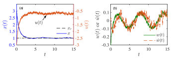
Figure 1: Trajectories of the state, control and total disturbance.

5.2 Control of an inverted pendulum

Consider a normalized model of the pendulum when the control input is the acceleration of the pivot (Åström et al., 2008):

$$\dot{x}_{1}=x_{2},\,\,\dot{x}_{2}=\sin x_{1}-u\cos x_{1}+w_{0},$$ (32)

where $x_{1}$ is the angular position of the pendulum with the origin at the upright position, $x_{2}$ is the angular velocity of the pendulum, and $w_{0}$ is an unknown disturbance which is equal to 0 if $t\leq 10$ and to $\sin t$ if $t>10$. The goal is to design a controller based on the measurable states $x_{1}$ and $x_{2}$ which stabilizes the pendulum at the upright position.

Specify the reference closed-loop model as: $\dot{x}_{r,\,1}=x_{r,\,2}$ and $\dot{x}_{r,\,2}=-k_{1}x_{r,\,1}-k_{2}x_{r,\,2}$, where $k_{1}$ and $k_{2}$ are positive scalars, and the desired tracking error dynamics as: $\dot{e}_{1}=e_{2}$ and $\dot{e}_{2}=-k_{1}e_{1}-k_{2}e_{2}$, where $e_{1}:=x_{r,\,1}-x_{1}$ and $e_{2}:=x_{r,\,2}-x_{2}$. Depending on the system model used, different controllers can be designed by the proposed approach.

Case A: The design bases on the ideal model (32) and ignores $w_{0}$, leading to the following control

$$u=(k_{1}x_{1}+k_{2}x_{2}+\sin x_{1})/\cos x_{1}.$$ (33)

It equals the control obtained by an input-output linearization technique (Srinivasan et al., 2009). The singularity of the control at $x_{1}=\frac{2k+1}{2}\pi$ for $k=0,\,1,\,2,\,...$, can be resolved by bounding the input and meanwhile switching the reference value of $x_{1}$ properly (Srinivasan et al., 2009). This controller is treated as a reference controller without explicit compensation for the unknown disturbance.

Case B: The dynamic model of $x_{2}$ is replaced by a fictitious model: $\dot{x}_{2}=-\alpha u+w$, where $w$ lumps any model mismatch (i.e., $w=\sin x_{1}+u(\alpha-\cos x_{1})+w_{0}$) and $\alpha$ is a given scalar which controls the mismatch. If a Type-I estimator is applied, it leads to an estimated control:

$$\hat{u}=\mathcal{L}^{-1}\left(\dfrac{k_{1}X_{1}+(k_{2}+sF_{x})X_{2}}{\alpha(1-F_{u})}\right),$$ (34)

where $F_{x}$ and $F_{u}$ are filters for estimating $\dot{x}_{2}$ and $u$, respectively. Note that the disturbance $w$ has been estimated and compensated in an implicit manner. If a Type-II estimator is used instead, then the estimate $\hat{w}$ is obtained from an ESO defined in (13) and the observer gain matrix $\bar{\mathbf{L}}\in\mathbb{R}^{3\times 2}$ is designed such that $\mathbf{\bar{A}-\bar{L}\bar{C}}$ is Hurwitz. The control then takes the form of

$$\hat{u}=(k_{1}x_{1}+k_{2}x_{2}+\hat{w})/\alpha.$$ (35)

The three controllers in (33), (34) and (35) are named as controllers A, B.I and B.II, respectively. The design parameters of the controllers are specified as: $k_{1}=k_{2}=2$, $\left|u_{\text{max}}\right|=5$ (bounded control), and $F_{x}=F_{u}=1/(0.05s+1)$. The filters $F_{x}$ and $F_{u}$ are such that the derivative of state $x_{2}$ can well be estimated, and the observer gain matrix $\bar{\mathbf{L}}$ is a function of $\alpha$ such that the three poles of the ESO are placed at -20, -20 and -40, which are ten or more times faster than the actual state dynamics.

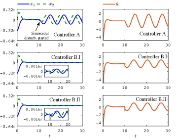
Figure 2: Performances of the three controllers.

With $(x_{1}(0),\,x_{2}(0))=(-\pi/3,\,0)$ and noise-free measurements, the simulation results for $\alpha=0.1$ are shown in Fig. 2. In the absence of the sinusoid disturbance, all three controllers were able to stabilize the pendulum with comparable performances. When the sinusoid disturbance appeared, however, controller A led to large tracking errors, in sharp contrast to controllers B.I and B.II. Further simulations show that the small tracking errors of controllers B.I and B.II were maintained if the measurements were corrupted with additive zero-mean Gaussian noises, while the controls were experiencing frequent variations. The results are not shown for brevity.

By varying the parameter $\alpha$, we simulated the control system with different degrees of model mismatches. The performances of controllers B.I and B.II are shown in Fig. 3(a)-(b). The integral absolute error (IAE) of state $x_{2}$ with respect to the origin and the integral variation (IV) of control $\hat{u}$ are used as the performance indices. Smaller IAE and IV indicate a better control performance. As observed, the IAE of $x_{2}$ increases as $\alpha$ is enlarged from 0.1 to 1.0, and so does the IV of $\hat{u}$ in most of the range, both of which indicate a degrading performance. This is somehow counterintuitive since a better performance were expected when the model tends to be more accurate (note that, $\alpha\hat{u}\rightarrow\hat{u}\cos x_{1}$ as $x_{1}\rightarrow 0$ and $\alpha\rightarrow 1$). The underlying fact is that the affine control component, $\hat{u}(\alpha-\cos x_{1})$, of the model mismatch $w$ acts to counteract the remaining mismatch, $\sin x_{1}+w_{0}$. As $\alpha$ approaches 1, the factor ($\alpha-\cos x_{1}$) approaches zero and hence the affine control component tends to be nullified. Consequently, this weakens the counteraction action and results in a larger total disturbance and a notable estimation error. This is reflected in the results shown in Fig. 3(c)-(d), in which the disturbance component $(\sin x_{1}+w_{0})$ is almost unchanged as $\alpha$ is changed from 0.1 to 1.

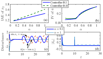
Figure 3: Performances of controllers B.I and B.II with different values of $\alpha$. (a)-(b): the performances of state tracking and control input vs. $\alpha$; (c)-(d): the evolutions of disturbance components and absolute disturbance estimation errors when controller B.II was implemented. Meanwhile, the IAE of $x_{2}$ and the IV of $u$ under controller A were obtained as 6.71 and 0.28, respectively.

6 Conclusions

This work presented an output feedback approach for controlling a general MIMO system to track a reference state trajectory. The approach uses a composite observer to estimate the system states and disturbances simultaneously, and then uses the estimates to derive the control. As the disturbances lump all unmodeled dynamics and are compensated online, the design admits a crude system model to be used for the control purpose. The closed-loop stability was established under some standard conditions.

It is desirable to analyze the closed-loop performance and extend the design to broader classes of systems such as those with time delays. It is also of interest to thoroughly investigate the interplay between state control and disturbance compensation, and then optimize the joint design. Future research may also consider embedding explicit disturbance compensation into existing control methods, such as robust control, optimal control, predictive control, etc., for obtaining flexible and enhanced controls.

References

References

- Åström & Wittenmark (2013) Åström, K. J., & Wittenmark, B. (2013). Adaptive control. Courier Corporation.
- Chen (1999) Chen, C. T. (1999). Linear System Theory and Design. Oxford: Oxford University Press.
- Chen et al. (2016) Chen, W.-H., Yang, J., Guo, L., & Li, S. (2016). Disturbance-observer-based control and related methods–an overview. IEEE Trans. Ind. Electron., 63, 1083–1095.
- Fliess (1990) Fliess, M. (1990). Generalized controller canonical form for linear and nonlinear dynamics. IEEE Trans. on Automatic Control, 35, 994–1001.
- Fliess & Join (2009) Fliess, M., & Join, C. (2009). Model-free control and intelligent pid controllers: towards a possible trivialization of nonlinear control? In 15th IFAC Symp. System Identif.. Saint-Malo.
- Fliess & Join (2013) Fliess, M., & Join, C. (2013). Model-free control. Inter. J. of Contr., 86, 2228–2252.
- Fliess & Sira-Ramírez (2003) Fliess, M., & Sira-Ramírez, H. (2003). An algebraic framework for linear identification. ESAIM: Control, Optimization and Calculus of Variations, 9, 151–168.
- Fliess & Sira-Ramírez (2008) Fliess, M., & Sira-Ramírez, H. (2008). Closed-loop parametric identification for continuous-time linear systems via new algebraic techniques. chapter 13 in Identification of Continuous-time Models from Sampled Data. (pp. 363–391). London: Springer Verlag.
- Gao (2006) Gao, Z. (2006). Active disturbance rejection control: a paradigm shift in feedback control system design. In American Control Conference.
- Gao (2014) Gao, Z. (2014). On the centrality of disturbance rejection in automatic control. ISA transactions, 53, 850–857.
- Guo & Zhao (2011) Guo, B.-Z., & Zhao, Z.-L. (2011). On the convergence of an extended state observer for nonlinear systems with uncertainty. Systems & Control Letters, 60, 420–430.
- Guo & Zhao (2013) Guo, B.-Z., & Zhao, Z.-L. (2013). On convergence of the nonlinear active disturbance rejection control for MIMO systems. SIAM Journal on Control and Optimization, 51, 1727–1757.
- Guo & Cao (2014) Guo, L., & Cao, S. (2014). Anti-disturbance control theory for systems with multiple disturbances: A survey. ISA Trans., 53, 846–849.
- Guo & Chen (2005) Guo, L., & Chen, W.-H. (2005). Disturbance attenuation and rejection for systems with nonlinearity via DOBC approach. Intl. J. Robust Nonlinear Control, 15, 109–125.
- Han (1981) Han, J. (1981). The structure of linear control system and computation in feedback system. (presented at the national meeting on control theory and applications, xiamen, 1979.). In Proceedings of the National Meeting on Control Theory and Applications, Science Press [in Chinese].
- Han (1995) Han, J. (1995). A class of extended state observers for uncertain systems. Control and Decision, 10, 85–88.
- Han (1998) Han, J. (1998). Auto-disturbance rejection control and its applications. Control and Decision, 13, 19–23.
- Han (1999) Han, J. (1999). Nonlinear design methods for control systems. In Proc. of the 14th IFAC World Congress (pp. 521–526).
- Hu et al. (2014) Hu, W., Camacho, E. F., & Xie, L. (2014). Feedforward and feedback control of dynamic systems. IFAC Proceedings Volumes, 47, 7741–7748.
- Hu & Mao (2014) Hu, W., & Mao, J. (2014). Improved algebraic method for linear continuous-time model identification. Journal of Control and Decision, 1, 180–189.
- Huang & Xue (2012) Huang, Y., & Xue, W. (2012). Active disturbance rejection control: methodology, applications and theoretical analysis. Journal of Systerms Science & Mathematical Sciences, 32, 1287–1307.
- Johnson (1968) Johnson, C. (1968). Optimal control of the linear regulator with constant disturbances. IEEE Trans. on Auto. Cont., 13, 416–421.
- Johnson (1970) Johnson, C. (1970). Further study of the linear regulator with disturbances–the case of vector disturbances satisfying a linear differential equation. IEEE Trans. on Auto. Cont., 15, 222–228.
- Johnson (1975) Johnson, C. (1975). On observers for systems with unknown and inaccessible inputs. Inter. J. of Contr., 21, 825–831.
- Johnson (1976) Johnson, C. (1976). Control and dynamic systems: Advances in theory and applications. chapter Theory of disturbance-accommodating controllers. (pp. 387–489). New York: Academic Press, Inc.
- Johnson (1986) Johnson, C. (1986). Disturbance-accommodating control: an overview. In American Control Conference (pp. 526–536).
- Kano & Ogawa (2010) Kano, M., & Ogawa, M. (2010). The state of the art in chemical process control in Japan: Good practice and questionnaire survey. Journal of Process Control, 20, 969–982.
- Khalil (2002) Khalil, H. K. (2002). Nonlinear Systems. (3rd ed.). Upper Saddle River, NJ: Prentice Hall.
- Madonski & Herman (2013) Madonski, R., & Herman, P. (2013). On the usefulness of higher-order disturbance observers in real control scenarios based on perturbation estimation and mitigation. In 9th Workshop on Robot Motion and Control (pp. 252–257).
- Meditch & Hostetter (1974) Meditch, J., & Hostetter, G. (1974). Observers for systems with unknown and inaccessible inputs. Inter. J. of Contr., 19, 473–480.
- Miklosovic et al. (2006) Miklosovic, R., Radke, A., & Gao, Z. (2006). Discrete implementation and generalization of the extended state observer. In American Control Conference.
- O’Dwyer (2009) O’Dwyer, A. (2009). Handbook of PI and PID Controller Tuning Rules. (3rd ed.). London: Imperial College Press.
- Ohishi et al. (1987) Ohishi, K., Nakao, M., Ohnishi, K., & Miyachi, K. (1987). Microprocessor-controlled dc motor for load-insensitive position servo system. IEEE Trans. Ind. Electron., (pp. 44–49).
- Ohishi et al. (1983) Ohishi, K., Ohnishi, K., & Miyachi, K. (1983). Torque-speed regulation of dc motor based on load torque estimation. In Proceedings of the IEEJ International Power Electronics Conference (pp. 1209–1216). volume 2.
- Patel & Toda (1980) Patel, R., & Toda, M. (1980). Quantitative measures of robustness for multivariable systems. In Joint Automatic Control Conference. San Francisco, CA, USA.
- Åström et al. (2008) Åström, K. J., Aracil, J., & Gordillo, F. (2008). A family of smooth controllers for swinging up a pendulum. Automatica, 44, 1841–1848.
- Sariyildiz & Ohnishi (2014) Sariyildiz, E., & Ohnishi, K. (2014). A guide to design disturbance observer. ASME J. Dyn. Syst., Meas., Control, 136, 021011.
- Schrijver & Van Dijk (2002) Schrijver, E., & Van Dijk, J. (2002). Disturbance observers for rigid mechanical systems: equivalence, stability, and design. ASME J. Dyn. Syst., Meas., Control, 124, 539–548.
- Shim & Jo (2009) Shim, H., & Jo, N. H. (2009). An almost necessary and sufficient condition for robust stability of closed-loop systems with disturbance observer. Automatica, 45, 296–299.
- Shim et al. (2008) Shim, H., Jo, N. H., & Son, Y.-I. (2008). A new disturbance observer for non-minimum phase linear systems. In American Control Conference (pp. 3385–3389). IEEE.
- Srinivasan et al. (2009) Srinivasan, B., Huguenin, P., & Bonvin, D. (2009). Global stabilization of an inverted pendulum - control strategy and experimental verification. Automatica, 45, 265–269.
- Truxall (1955) Truxall, J. G. (1955). Automatic feedback control system synthesis. MacGraw-Hill.
- Yang & Huang (2009) Yang, X., & Huang, Y. (2009). Capabilities of extended state observer for estimating uncertainties. In American Control Conference (pp. 3700–3705).
- Yao & Guo (2014) Yao, X., & Guo, L. (2014). Disturbance attenuation and rejection for discrete-time markovian jump systems with lossy measurements. Info. Sciences, 278, 673–684.
- Youcef-Toumi & Ito (1988) Youcef-Toumi, K., & Ito, O. (1988). A time delay controller for systems with unknown dynamics. In American Control Conference (pp. 904–913).
- Zheng et al. (2007) Zheng, Q., Gao, L. Q., & Gao, Z. (2007). On stability analysis of active disturbance rejection control for nonlinear time-varying plants with unknown dynamics. In 46th IEEE Conference on Decision and Control (pp. 3501–3506).
- Zheng et al. (2012) Zheng, Q., Gao, L. Q., & Gao, Z. (2012). On validation of extended state observer through analysis and experimentation. ASME J. Dyn. Syst., Meas., Control, 134, 024505–1–6.
- Zhong et al. (2011) Zhong, Q.-C., Kuperman, A., & Stobart, R. (2011). Design of ude-based controllers from their two-degree-of-freedom nature. Inter. J. of Robust and Nonlinear Contr., 21, 1994–2008.
- Zhong & Rees (2004) Zhong, Q.-C., & Rees, D. (2004). Control of uncertain LTI systems based on an uncertainty and disturbance estimator. ASME J. Dyn. Syst., Meas., Control, 126, 905–910.
- Zhou & Doyle (1998) Zhou, K., & Doyle, J. C. (1998). Essentials of Robust Control. Prentice Hall Upper Saddle River, NJ.