Abstract

Spatiotemporal patterns such as traveling waves are frequently observed in recordings of neural activity. The mechanisms underlying the generation of such patterns are largely unknown. Previous studies have investigated the existence and uniqueness of different types of waves or bumps of activity using neural-field models, phenomenological coarse-grained descriptions of neural-network dynamics. But it remains unclear how these insights can be transferred to more biologically realistic networks of spiking neurons, where individual neurons fire irregularly. Here, we employ mean-field theory to reduce a microscopic model of leaky integrate-and-fire (LIF) neurons with distance-dependent connectivity to an effective neural-field model. In contrast to existing phenomenological descriptions, the dynamics in this neural-field model depends on the mean and the variance in the synaptic input, both determining the amplitude and the temporal structure of the resulting effective coupling kernel. For the neural-field model we employ liner stability analysis to derive conditions for the existence of spatial and temporal oscillations and wave trains, that is, temporally and spatially periodic traveling waves. We first prove that wave trains cannot occur in a single homogeneous population of neurons, irrespective of the form of distance dependence of the connection probability. Compatible with the architecture of cortical neural networks, wave trains emerge in two-population networks of excitatory and inhibitory neurons as a combination of delay-induced temporal oscillations and spatial oscillations due to distance-dependent connectivity profiles. Finally, we demonstrate quantitative agreement between predictions of the analytically tractable neural-field model and numerical simulations of both networks of nonlinear rate-based units and networks of LIF neurons.

1 Introduction

Experimental recordings of neural activity frequently reveal spatiotemporal patterns such as traveling waves propagating across the cortical surface [1, 2, 3, 4, 5, 6, 7, 8] or within other brain regions such as the thalamus [9, 3] or the hippocampus [10]. These large-scale dynamical phenomena are detected in local-field potentials (LFP) [11] and in the spiking activity [12] recorded with multi-electrode arrays, by voltage-sensitive dye imaging [13], or by two-photon imaging monitoring the intracellular calcium concentration [14]. They have been reported in in-vitro and in in-vivo experiments, in both anesthetized and awake states, and during spontaneous as well as stimulus-evoked activity [3].

Previous modeling studies have shown that networks of spiking neurons with distance-dependent connectivity, extending in one- or two-dimensional space, can exhibit a variety of such spatiotemporal patterns [15, 16, 17, 18]. For illustration, consider the example in Fig 1. Depending on the choice of transmission delays, the spatial reach of connections and the strength of inhibition, a network of leaky integrate-and-fire (LIF) model neurons generates asynchronous-irregular activity (A), spatial patterns that are persistent in time (B), spatially uniform temporal oscillations (C), or propagating waves (D). Distance-dependent connectivity is a prominent feature of biological networks. In the neocortex, local connections are established within a radius of about $500\,\mathrm{\mu m}$ around a neuron’s cell body [19], and the probability of two neurons being connected decays with distance [20, 21, 22].

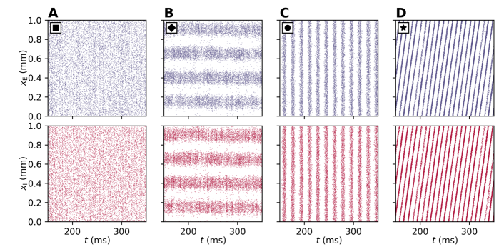
Figure 1: Spatiotemporal patterns in a spiking neural network model. Spiking activity of recurrently connected populations of excitatory ($\mathrm{E}$, blue) and inhibitory ($\mathrm{I}$, red) leaky integrate-and-fire neurons. Each dot represents the spike-emission time of a particular neuron. Neurons are positioned on a ring with a perimeter of $1\,\mathrm{mm}$. Each neuron receives a fixed number of incoming connections from its excitatory (inhibitory) neighbors uniformly and randomly drawn within a distance of $R_{\mathrm{E}}$ ($R_{\mathrm{I}}$). The spike-transmission delay $d$, the widths $R_{\mathrm{E}}$ and $R_{\mathrm{I}}$ of the spatial connectivity profiles, and the relative inhibitory synaptic weight $g$ are varied. A Asynchronous-irregular activity ($d=1\,\mathrm{ms}$, $R_{\mathrm{E}}=R_{\mathrm{I}}=0.4\,\mathrm{mm}$, $g=6$). B Oscillations in space ($d=3\,\mathrm{ms}$, $R_{\mathrm{E}}=0.1\,\mathrm{mm}$, $R_{\mathrm{I}}=0.15\,\mathrm{mm}$, $g=5$). C Oscillations in time ($d=6\,\mathrm{ms}$, $R_{\mathrm{E}}=R_{\mathrm{I}}=0.4\,\mathrm{mm}$, $g=7$). D Propagating waves ($d=3\,\mathrm{ms}$, $R_{\mathrm{E}}=0.2\,\mathrm{mm}$, $R_{\mathrm{I}}=0.07\,\mathrm{mm}$, $g=5$). For remaining parameters, see Table  4.

So far, the formation of spatiotemporal patterns in neural networks has mainly been studied by means of phenomenological neural-field models describing network dynamics at a macroscopic spatial scale [23, 24, 25]. Such models can describe patterns in recorded brain activity that are related to movement [26] or occur in response to a visual stimulus [27]. Neural-field models are formulated with continuous nonlinear integro-differential equations for a spatially and temporally resolved activity variable and usually possess an effective distance-dependent connectivity kernel. These models provide insights into the existence and uniqueness of diverse patterns which are stationary or nonstationary in space and time, such as waves, wave fronts, bumps, pulses, and periodic patterns (reviewed in [28, 29, 30, 31, 32, 33, 34]). There are two main techniques for analyzing spatiotemporal patterns in neural-field models [32]: First, in the constructive approach introduced by Amari [25], bump or wave solutions are explicitly constructed by relating the spatial and temporal coordinates of a nonlinear system (reviewed in [28, Section 7] and [32, Sections 3-4]). Second, the emergence of periodic patterns is studied with bifurcation theory as in the seminal works of Ermentrout and Cowan [35, 36, 37, 38]. In this latter framework, linear stability analysis is often employed to detect pattern-forming instabilities and to derive conditions for the onset of pattern formation (see for example [39, 40] or the reviews [28, Section 8] and [32, Section 5]). There are four general classes of states that can linearly bifurcate from a homogeneous steady state: a new uniform stationary state, temporal oscillations (spatially uniform and periodic in time, also known as global ‘bulk oscillations’ [41]), spatial oscillations (spatially periodic and stationary in time), and wave trains (spatially and temporally periodic; special type of traveling waves), see [28, Section 8] and [42, 43, 44]. The analysis of these states is often called ‘(linear) Turing instability analysis’ [29, 45, 44] referring to the work of Turing on patterns in reaction-diffusion systems [46]. The respective instabilities leading to these states are termed: a firing rate instability, Hopf instability [47], Turing instability, and Turing-Hopf [42] or ‘wave’ [40] instability. The instabilities generating temporally periodic patterns (Hopf and Turing-Hopf instabilities) are known as ‘dynamic’ [44] or ‘nonstationary’ [48] instabilities, in contrast to ‘static’ [44] or ‘stationary’ [48] instabilities generating temporally stationary patterns.

The emergence of pattern-forming instabilities has been investigated with respect to system parameters such as the spatial reach of excitation and inhibition in an effective connectivity profile [28]; specifically without transmission delays [49, 50], or with constant [42, 51], distance-dependent [52, 40, 53, 43, 45, 41, 54, 55, 56] or both types [57, 58] of delays. Faye and Faugeras[59] show existence and uniqueness of solutions and provide conditions for asymptotic stability of the trivial homogeneous steady state of the corresponding linearized system using the Lyapunov functional. The principle of linearized stability for such models was proven by Veltz and Faugeras [60]. Dijkstra et al. [61] provide a rigorous analysis of a one-dimensional neural-field model revealing pitchfork-Hopf bifurcations. The existence of standing waves emerging from a Turing bifurcation of the trivial homogeneous steady state, in a linearized neural field model with space-dependent delays on a sphere, was shown by Visser et al. [62].

Neural-field models treat neural tissue as a continuous excitable medium and describe neural activity in terms of a space and time dependent real-valued quantity. Throughout the current work the spatial coordinate refers to physical space, although in general it could also be interpreted as feature space. At the microscopic scale, in contrast, neural networks are composed of discrete units (neurons) – which interact via occasional short stereotypical pulses (spikes) rather than continuous quantities like firing rates. In the neocortex, spiking activity is typically highly irregular and sparse [63, 64], with weak pairwise correlations [65]. To date, a rigorous link between this microscopic level and the macroscopic description by neural-field models is lacking [31, 33, 66, 67]. While randomly connected spiking networks have been extensively analyzed using mean-field approaches [68, 64, 69, 70, 71], the theoretical understanding of spatially structured spiking networks is still deficient. A recent work in this direction is Esnaola-Acebes et al. [72], who investigate ring networks of quadratic integrate-and-fire model neurons and provide bifurcation diagrams showing temporal oscillations and bump states, supported by both mathematical analysis and simulation. But in general it remains unclear how to qualitatively transfer insights on the formation of spatiotemporal patterns from neural fields to networks of spiking neurons. Moreover, it is unknown how the multitude of neuron, synapse and connectivity parameters of spiking neural networks relates to the effective parameters in neural-field models. A quantitative link between the two levels of description is, for example, required for adjusting parameters in a network of spiking neurons such that it generates a specific type of spatiotemporal pattern, and to enable model validation by comparison with experimental data.

Different efforts have already been undertaken to match spiking and time-continuous rate models with spatial structure. Certain assumptions and approximations allow the application of techniques for analyzing spatiotemporal patterns developed for neural-field models. The above mentioned constructive approach [25], for example, can be applied to networks of spiking neurons under the assumption that every neuron spikes at most once, thus ignoring the sustained spike generation and after-spike dynamics of biological neurons [73, 74, 75]. A related simplification substitutes a spike train by an ansatz for a wave front. This leads to a mean-field description of single-spike activity often applied to a spike-response model [76, 77, 78, 79]. Traveling-wave solutions have also been proposed for a network of coupled oscillators and a corresponding continuum model [80]. In the framework of bifurcation theory, Roxin et al. [42, 51] demonstrate a qualitative agreement between a neural-field model and a numerically simulated network of Hodgkin-Huxley-type neurons in terms of emerging spatiotemporal patterns. However, the authors do not observe stable traveling waves in the spiking network, even though the neural-field model predicts their occurrence. In the limit of slow synaptic interactions, spiking dynamics can be reduced to a mean-firing-rate model for studying bifurcations [81, 82, 83]. An example is the lighthouse model [84, 85], defined as a hybrid between a phase oscillator and a firing-rate model, that reduces to a pure rate model for slow synapses [86]. Laing and Chow [87] demonstrate a bump solution in a spiking network and discuss a corresponding rate model. Recently, the group around Doiron and Rosenbaum explored in a sequence of studies spatially structured networks of LIF neurons without transmission delays in the continuum limit with respect to the spatial widths of connectivity. The authors focus on the existence of the balanced state [88], the structure of correlations in the spiking activity [89], and bifurcations in the linearized dynamics in relation to network computations [90]. Spreizer et al. [91] further demonstrate that spatiotemporal activity sequences can be induced by anisotropic but spatially correlated connectivity. Kriener et al. [92] employ static mean-field theory and extend the linearization of a network of LIF neurons with constant delays as described by Brunel [69], to spatially structured networks. The work derives conditions for the appearance of spontaneous symmetry breaking that leads to stationary periodic bump solutions (spatial oscillations), and distinguish between the mean-driven and the fluctuation driven regime. A coarse-graining procedure for a ring network of modified binary neurons with refractoriness was presented by Avitable and Wedgwood [93]. By combining analytical and numerical analysis they show existence of bumps and traveling waves.

Despite these previous works on spatially structured network models of spiking neurons and attempts to link them with neural-field models, there still exists no systematic way of mapping parameters between these models. Furthermore, none of these studies focuses on uncovering the underlying mechanism of wave trains in spiking networks. In the present work we establish the so far missing, quantitative link between a sparsely connected network of spiking LIF neurons with spatial structure and a typical neural-field model. An explicit parameter mapping between the two levels of description allows us to study the origin of spatiotemporal patterns analytically in the neural-field model using linear stability analysis, and to reproduce the predicted patterns in spiking activity. We employ mean-field theory to derive the neural-field model as an effective rate model depending on the dynamical working point of the network that is characterized by both the mean and the variance of the synaptic input. The rate model accounts for biological constraints such as a static weight that is either positive (excitatory) or negative (inhibitory) and a spatial profile that can be interpreted as a distance-dependent connection probability. Given these constraints, we show that wave trains cannot occur in a single homogeneous population irrespective of the shape of distance-dependent connection probability. For two-population networks of excitatory and inhibitory neurons, in contrast, wave trains emerge for specific types of spatial profiles and for sufficiently large delays, as shown in Fig 1D.

The remainder of the study is structured as follows: In Results we derive the conditions for the existence of wave trains for a typical neural-field model by linear stability analysis, present an effective model corresponding to the microscopic description of spiking neurons, compare the two models, and show simulation results for validation. In Discussion we put our results in the context of previous literature. Finally, Appendix contains details on our approach. An account of the presented work has previously been published in abstract form in [94].

2 Results

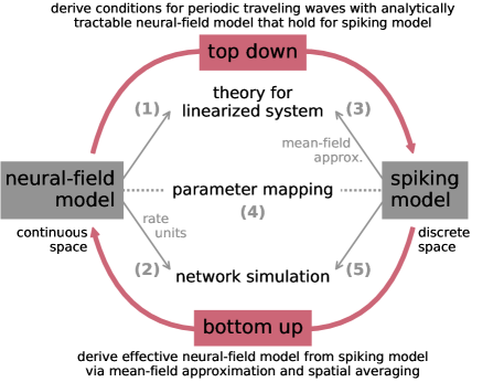
Figure 2: Mapping microscopic single-neuron dynamics to spatially averaged population dynamics. (1) Conditions for wave trains in a neural-field model. (2) Network simulation of discrete nonlinear rate neurons. (3) Mean-field approximation of the spiking model and spatial averaging lead to an effective linearized continuous system. (4) Parameter mapping between spiking and neural-field model. (5) Network simulation of spiking neurons and validation of analytical results.

We aim to establish a mapping between two different levels of description for spatially structured neural systems to which we refer as ‘neural-field model’ and ‘spiking model’ based on the initial model assumptions. While the neural-field model describes neural activity as a quantity that is continuous in space and time, the spiking model assumes a network of recurrently connected spiking model neurons in discrete space. Our methodological approach for mapping between these two models, as well as the structure of this section, are illustrated in Fig 2. (1) We start in Sections 2.1-2.3 with linear stability analysis of a typical neural-field model that is a well-known and analytically tractable rate equation. This approach builds on existing literature (cf. [28, Section 8] and [32, Section 5]) and introduces the concepts of our study with modest mathematical efforts. We analyze the neural-field model for one and two populations and derive conditions for the occurrence of wave trains based on spatial connectivity profiles and transmission delays. (2) In Section 2.4 we continue with simulations of a discrete version of the neural-field model, a network of nonlinear rate-based units, and show that the results from our linear analysis indeed accurately predict transitions between network states (homogeneously steady, spatial oscillations, temporal oscillations, waves). (3) Then, in Section 2.5 we linearize the population dynamics of networks of discrete spiking leaky integrate-and-fire (LIF) neurons using mean-field theory and derive expressions similar to the neural-field model. (4) Thus, both the linearized neural-field and spiking models can be treated in a conceptually similar manner, with the exception of an effective coupling kernel which is mathematically more involved for the spiking model. In Section 2.6 we perform a parameter mapping between the biophysically motivated parameters of the spiking model and the effective parameters of a neural-field model. (5) Finally, in Section 2.7 we demonstrate that the insights obtained in the analysis of the neural-field model apply to networks of simulated LIF neurons: The bifurcations indeed appear at the theoretically predicted parameter values.

In summary, the mapping of a microscopic spiking network model to a continuum neural-field model (bottom up) allows us to transfer analytically derived insights from the neural-field model directly to the spiking model (top down).

2.1 Linear stability analysis of a neural-field model

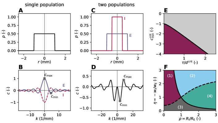
Figure 3: Effective profile yields conditions for wave trains. A Boxcar-shaped spatial profile $p$ of width $R=1\,\mathrm{mm}$ for a single population. B Effective profile $c$ (blue curve) denotes Fourier transform of spatial profile $\widehat{p}$ times positive weight $w_{\mathrm{E}}=1$. Gray crosses indicate maximum $\mathrm{c_{\mathrm{max}}}$ and minimum $c_{\mathrm{min}}$. Same spatial profile but with negative weight ($w_{\mathrm{I}}=-w_{\mathrm{E}}$) yields mirrored curve (red, dashed line). C Spatial profiles of different widths for two populations $\mathrm{E}$ ($R_{\mathrm{E}}=1\,\mathrm{mm}$, blue) and $\mathrm{I}$ ($R_{\mathrm{I}}=0.5\,\mathrm{mm}$, red). D Effective profile: $c\left(k\right)=w_{\mathrm{E}}\widehat{p}_{\mathrm{E}}\left(k\right)+w_{\mathrm{I}}\widehat{p}_{\mathrm{I}}\left(k\right)$. E Transition curve $c_{\mathrm{min}}^{\mathrm{crit}}(\tau/d^{\mathrm{crit}})$ given by Eq 10 for Hopf bifurcation indicating onset of delay-induced oscillations (appearing in purple region) with time constant $\tau$ and delay $d$. F Transition curves for relative width $\rho=R_{\mathrm{I}}/R_{\mathrm{E}}$ and relative weight $\eta=-w_{\mathrm{I}}/w_{\mathrm{E}}$. Colored regions indicate which extremum, the minimum $c_{\mathrm{min}}$ or the maximum $c_{\mathrm{max}}$, has larger absolute value and if the dominant one occurs at $k=0$ or at $k>0$. Purple (1): $c_{\mathrm{min}}$ appears at $k_{\mathrm{min}}>0$. Light blue (2): $c_{\mathrm{min}}$ appears at $k_{\mathrm{min}}=0$. Dark gray (3): $c_{\mathrm{max}}$ appears at $k_{\mathrm{max}}=0$. Green (4) $c_{\mathrm{max}}$ appears at $k_{\mathrm{max}}>0$.

We first consider a neural-field model with a single population defined as a continuous excitable medium with a translation-invariant interaction kernel and delayed interaction in one spatial dimension. The dynamics follows an integro-differential equation

$$\tau\,\frac{\partial u}{\mathrm{\partial}t}\left(x,t\right)+u\left(x,t\right)=\int_{-\infty}^{\infty}m\left(x-y\right)\,\psi\left(u\left(y,t-d\right)\right)\,\mathrm{d}y.$$ (1)

The variable $u$ describes the activity of the neural population at position $x$ at time $t$. Here $\tau>0$ denotes a time constant and $d>0$ a transmission delay. The function $\psi$ describes the nonlinear transformation of the output activity $u$ if considered as input to the neural field. The function $m$ specifies the translation-invariant connectivity depending only on the displacement $r=x-y$ where $x$ and $y$ denote neuron positions. Earlier studies show that specific choices for connectivities $P$ and nonlinear transformations $\psi$ result in spatiotemporal patterns such as waves or bumps [28, 29, 30, 31, 32, 33, 34].

Here, we assume that the connectivity $m$ is isotropic and define $m\left(r\right)\coloneqq w\,p\left(r\right)$. The scalar weight $w$ can either be positive (excitatory) or negative (inhibitory). The spatial profile $p(r)$ is a symmetric probability density function with the properties $p\left(r\right)=p\left(-r\right)$, $p(r)>0$ for $r\in\left(-\infty,\infty\right)$ and $\int_{-\infty}^{\infty}p\left(r\right)\,\mathrm{d}r=1$. Fig 3A shows, as an example, a boxcar-shaped spatial profile with width $R$, defined by $p\left(r\right)=\frac{1}{2R}\Theta\left(R-\left|r\right|\right)$ where $\Theta$ denotes the Heaviside function.

Throughout this study we investigate bifurcations of the system Eq 1 between a state of spatially and temporally homogeneous activity $u(x,t)=u_{0}$ to states where the activity shows structure in the temporal domain, in the spatial domain, or both. For this purpose we use Turing instability analysis [39, 40, 29]. Initially we assume that the model parameters are chosen such that the homogeneous solution is locally asymptotically stable, implying that small perturbations away from $u_{0}$ will relax back to this baseline. We ask the question: In which regions of the parameter space ($R$, $d$, $w$, $\psi$) is the stability of the homogeneous solution lost? To this end we linearize around the steady state and denote deviations $\delta u(t)=u(t)-u_{0}$. Without loss of generality we assume the slope $\psi^{\prime}(u_{0})$ of the gain function to be unity; a non-zero slope can be absorbed into a redefinition of $w$. We here use a gain function that allows $u$ to become negative. Likewise, one can treat nonlinear gain functions $\psi$ that are strictly positive (see, e.g., [51]). These two conventions can be mapped to one another by a suitable shift of variables. In either case, after linearization the deviation $\delta u$ does not have a definite sign. Because the resulting linear system is invariant with respect to translations in time and space, its eigenmodes are Fourier-Laplace modes of the form

$$\delta u\left(x,t\right) =\mathrm{e}^{\mathrm{i}kx}\mathrm{e}^{\lambda t},$$ (2)

where the wave number $k\in\mathbb{R}$ is real and the temporal eigenvalue $\lambda\in\mathbb{C}$ is complex. Solutions constructed from these eigenmodes can oscillate in time and space, and exponentially grow or decay in time. The characteristic equation (see Eq 33 in Appendix)

$$\left(1+\tau\lambda\right)\,\mathrm{e}^{\lambda d}=c\left(k\right),$$ (3)

comprises the effective profile $c\left(k\right)\coloneqq\widehat{m}\left(k\right)\coloneqq w\widehat{p}\left(k\right)$. The Fourier transform of the spatial profile is denoted by $\widehat{p}\left(k\right)$ which, by its definition as a probability density, is maximal at $k=0$ with $\widehat{p}\left(0\right)=1$ (see Eqs 40 and 41 in Appendix). The effective profile for the boxcar-shaped spatial profile is shown in Fig 3B, for excitatory and inhibitory weights with absolute magnitudes of unity.

We next extend the system to two populations, an excitatory one denoted by $\mathrm{E}$, and an inhibitory one by $\mathrm{I}$. Time constants $\tau$ and delays $d$ are assumed to be equal for both populations, but $u$ becomes a vector, $u=\left(u_{\mathrm{E}},u_{\mathrm{I}}\right)^{T}$, and the connectivity $m\left(r\right)$ a matrix

$$M\left(r\right)=\left(\begin{array}[]{cc}w_{\mathrm{EE}}\,p_{\mathrm{EE}}\left(r\right)&w_{\mathrm{EI}}\,p_{\mathrm{EI}}\left(r\right)\\ w_{\mathrm{IE}}\,p_{\mathrm{IE}}\left(r\right)&w_{\mathrm{II}}\,p_{\mathrm{II}}\left(r\right)\end{array}\right).$$ (4)

The linearized system again possesses the same symmetries as the counterpart for a single population so that the eigenmodes for the deviation from the stationary state are of the form $\delta u\left(x,t\right)=ve^{\mathrm{i}kx}\mathrm{e^{\lambda t}}$ with $v$ denoting a constant vector. Hence, we arrive at an auxiliary eigenvalue problem (see Eq 34 in Appendix) with the two eigenvalues

$$c_{1,2}\left(k\right)=\frac{1}{2}\left(w_{\mathrm{EE}}\,\widehat{p}_{\mathrm{EE}}\left(k\right)+w_{\mathrm{II}}\,\widehat{p}{}_{\mathrm{II}}\left(k\right)\pm\sqrt{D}\right),$$ (5)

where

$$D=\left(w_{\mathrm{EE}}\,\widehat{p}_{\mathrm{EE}}\left(k\right)-w_{\mathrm{II}}\,\widehat{p}_{\mathrm{II}}\left(k\right)\right)^{2}+4w_{\mathrm{EI}}\,\widehat{p}_{\mathrm{EI}}\left(k\right)\,w_{\mathrm{IE}}\,\widehat{p}_{\mathrm{IE}}\left(k\right).$$ (6)

These two eigenvalues play the same role as the effective profile $c$ in the one-population case above. As a consequence, the same characteristic equation Eq 3 holds for both the one- and the two-population system, as a scalar and two-dimensional vector equation, respectively.

In the following example we restrict the weights and the spatial profiles to be uniquely determined by the source population alone, denoted by $w_{\mathrm{\alpha E}}=:w_{\mathrm{E}}$, $w_{\mathrm{\alpha I}}=:w_{\mathrm{I}}$ for $\alpha\in\{\mathrm{E},\mathrm{I}\}$. An illustration of the two spatial profiles of different widths $R_{\mathrm{E}}$ and $R_{\mathrm{I}}$ is shown in Fig 3C. The respective effective profile Eq 5 reduces to $c_{1}\left(k\right)=w_{\mathrm{E}}\widehat{p}_{\mathrm{E}}\left(k\right)+w_{\mathrm{I}}\widehat{p}_{\mathrm{I}}\left(k\right)=:c\left(k\right)$, and is shown in Fig 3D; $c_{2}\equiv 0$ for all $k.$

The characteristic equation Eq 3 can be solved for the eigenvalues $\lambda$ by using the Lambert W function defined as $z=W\left(z\right)\mathrm{e}^{W\left(z\right)}$ for $z\in\mathbb{C}$ [95]. The Lambert W function has infinitely many branches, indexed by $b$, and the branch with the largest real part is denoted the principle branch ($b=0$), see Eqs 37-38 in Appendix for a proof. The characteristic equation determines the temporal eigenvalues (see Eq 39 in Appendix and compare with [58])

$$\lambda_{b}(k)=-\frac{1}{\tau}+\frac{1}{d}\,W_{b}\left(c\left(k\right)\frac{d}{\tau}\mathrm{e}^{\frac{d}{\tau}}\right).$$ (7)

As shown by Veltz and Faugeras [60], linearized stability of the homogeneous steady state of Eq 1 is fully determined by the eigenvalues Eq 7. These authors assume an open bounded domain and provide an example of a one-dimensional ring network. In our theoretical analysis, we decide to work with the infinite domain for technical convenience. Formulating the problem on a ring with periodic boundary conditions would not change any of our conclusions. The added value of their approach is the possibility to justify all steps in a mathematically rigorous way. In our approach, the temporal eigenvalue $\lambda_{b}$ is a continuous function of the wave number $k.$ On a bounded domain with periodic boundary conditions, one obtains a discrete set of wave numbers $k$. Since the temporal eigenvalue $\lambda_{b}$ varies on a much slower scale compared to the resolution of discrete wave numbers $k$, this change does not have any qualitative effect on the resulting dynamics. The infinite domain, however, allows us to easily incorporate spatial profiles with unbounded support. For profiles with unbounded support that decay to zero fast enough, the theoretical prediction of the frequency of oscillation can be regarded as an approximation of the dynamics on a ring with periodic boundary conditions.

2.2 Conditions for spatial and temporal oscillations, and wave trains

The homogeneous (steady) state of our system is locally asymptotically stable if the real parts of all eigenvalues $\lambda_{b}$ are negative

$$\operatorname{Re}\left[W_{b}\left(c\left(k\right)\frac{d}{\tau}\mathrm{e}^{\frac{d}{\tau}}\right)\right]<\frac{d}{\tau},{\normalcolor}$$ (8)

for all branches $b$ of the Lambert W function. The system loses stability when the real part of the eigenvalue $\lambda_{0}$ on the principle branch becomes positive at a certain $k=k^{*}$. Such instabilities may occur either for a positive or a negative argument of the Lambert W function.

We denote the maximum of $c$ as $c_{\mathrm{max}}$ and the minimum as $\mathrm{c_{\mathrm{min}}}$ occurring at $k_{\mathrm{max}}$ and $k\mathrm{{}_{min}}$, respectively, as indicated in Fig 3B and D. The system becomes unstable for a positive argument of $W$ if $c_{\mathrm{max}}=1$ where $W\left(\frac{d}{\tau}\mathrm{e}^{\frac{d}{\tau}}\right)=\frac{d}{\tau}$ by the definition of the Lambert W function; so equality holds in Eq 8 independent of the values $d$ and $\tau$. The imaginary part of $\lambda_{0}$ is zero at such a transition because the principal branch of the Lambert W function has real values for positive real arguments. If the instability appears at a wave number $k^{\ast}=0$, the population activity is collectively destabilized. This transition corresponds in networks of binary neurons and of spiking neurons to the transition between the asynchronous irregular (AI) state and the synchronous regular (SR) state, where the system ceases to be stabilized by negative feedback and leaves the balanced state [96, 69]. If this transition appears at a wave number $k^{*}>0$, it follows from Eq 2 that the activity shows spatial oscillations that grow exponentially in time.

For a negative argument of $W$ of less than $-1/e$, the eigenvalues Eq 7 come in complex conjugate pairs. The real part of $\lambda_{0}$ becomes positive if the condition

$$\operatorname{Re}\left[W_{0}\left(c_{\mathrm{min}}\frac{d}{\tau}\mathrm{e}^{\frac{d}{\tau}}\right)\right]=\frac{d}{\tau}$$ (9)

is fulfilled with a negative $c_{\mathrm{min}}<-1$. Because the eigenvalues have non-zero imaginary parts, this transition corresponds to a Hopf bifurcation and the onset of temporal oscillations. The condition for this bifurcation has been derived earlier [97, Eq 10]

$$\frac{d^{\mathrm{crit}}}{\tau}=\frac{\pi-\arctan\left(\sqrt{c_{\mathrm{min}}^{\mathrm{crit^{2}}}-1}\right)}{\sqrt{c_{\mathrm{min}}^{\mathrm{crit}^{2}}-1}}.$$ (10)

Here, $d^{\mathrm{crit}}$ denotes the critical delay and $c_{\mathrm{min}}^{\mathrm{crit}}$ a critical minimum of the effective profile for points on the transition curve. The system is stable for $c_{\mathrm{min}}>-1$ for all delays. For larger absolute values of $c_{\mathrm{min}}$, the bifurcation point is given by the critical value of the ratio between the time constant and the delay, shown in Fig 3E. If the transition occurs at $k^{\ast}=0$, temporal oscillations emerge in which all neurons of the population oscillate in phase (‘bulk oscillations’ [41]). In spiking networks this Hopf bifurcation corresponds to the transition from the AI regime to the state termed ‘synchronous irregular fast (SI fast)’ [64]. If the transition appears for $k^{*}>0$, spatial and temporal oscillations occur simultaneously. This phenomenon is known as ‘wave trains’, see [28, Section 8] and [42, 43, 44]. For the case that the system becomes unstable due to $c_{\mathrm{max}}$ reaching unity, the transition curve in Fig 3E also provides a lower bound $c_{\mathrm{min}}^{\mathrm{crit}}(\tau/d^{\mathrm{crit}})$ above which temporal oscillations do not occur prior to the transition due to $c_{\mathrm{max}}$.

A Hopf bifurcation can give rise to either an asymptotically stable or unstable limit cycle, in the super- or subcritical case, respectively. In our analysis we only identify the Hopf bifurcation point by checking when a complex conjugate pair of eigenvalues crosses the imaginary axis, and therefore cannot predict the stability of the emerging limit cycle. If we, however, in the simulation observe the transition from an asymptotically stable homogeneous steady state, corresponding to the asynchronous irregular regime, to spatiotemporal patterns, corresponding to a stable limit cycle, and make sure that the initial conditions are close enough to the homogeneous steady state, we know that the bifurcation we see is indeed a supercritical Hopf bifurcation. The analytical conditions for wave trains that we derive are necessary, but not sufficient.

	homogeneous	spatial oscillations	temporal oscillations	wave trains
$c_{\mathrm{max}}$	$<1$	$1$	$<1$	$<1$
$c_{\mathrm{min}}$	$>c_{\mathrm{min}}^{\mathrm{crit}}$	$>c_{\mathrm{min}}^{\mathrm{crit}}$	$c_{\mathrm{min}}^{\mathrm{crit}}$	$c_{\mathrm{min}}^{\mathrm{crit}}$
$d$	$<d^{\mathrm{crit}}$	$<d^{\mathrm{crit}}$	$d^{\mathrm{crit}}$	$d^{\mathrm{crit}}$
$k^{*}$	-	$>0$	$0$	$>0$

Table 1: Conditions for the onset of spatial and temporal oscillations, and wave trains. Gray cells in each column indicate the conditions required for the instability causing the bifurcation. White cells denote the conditions for the respective other bifurcation not to occur. Last row indicates whether the bifurcation happens for zero or nonzero wave number $k^{*}$. Here $d^{\mathrm{crit}}$ and $c_{\mathrm{min}}^{\mathrm{crit}}$, as defined in Eq 10 and shown in Fig 3E, denote the critical delay and the minimum of the effective profile on the transition curve for a Hopf bifurcation.

In summary, the system is stable if $c_{\mathrm{max}}<1$ and $c_{\mathrm{min}}>c_{\mathrm{min}}^{\mathrm{crit}}(\tau/d^{\mathrm{crit}})$. For transitions occurring at either $c_{\mathrm{max}}=1$ or $c_{\mathrm{min}}=c_{\mathrm{min}}^{\mathrm{crit}}(\tau/d^{\mathrm{crit}})$ we distinguish between solutions with $k^{*}=0$ or $k^{*}>0$. In Table  1 we provide an overview of the conditions for bifurcations leading to spatial, temporal, or spatiotemporal oscillatory states. These conditions imply that a one-population neural-field model does not permit wave trains, which follows from the fact that the absolute value of $\widehat{p}$ is strictly maximal at $k=0$ (see Eqs 40–41 in Appendix). For a purely excitatory population ($w>0$) the critical minimum $c_{\mathrm{min}}^{\mathrm{crit}}(\tau/d^{\mathrm{crit}})$ therefore cannot be reached while keeping the maximum $c_{\mathrm{max}}$ stable as $c_{\mathrm{max}}>\left|c_{\mathrm{min}}\right|$. For a purely inhibitory population ($w<0$), the condition $k_{\mathrm{min}}>0$ is not fulfilled because $c_{\mathrm{min}}$ occurs at $k=0$ as $\widehat{p}$ has its global maximum at the origin.

For a neural-field model accounting for both excitation and inhibition, however, we can select shapes and parameters of the spatial profiles, weights and the delay that fulfill the conditions for the onset of wave trains as demonstrated by example in the next section.

2.3 Application to a network with excitatory and inhibitory populations

Based on the conditions derived in the previous section, the minimal network in conformity with Dale’s principle in which wave trains can occur consists of one excitatory ($\mathrm{E}$) and one inhibitory ($\mathrm{I}$) population. As in the example in Section 2.1, we assume that the connection weights and widths of boxcar-shaped spatial profiles only depend on the source population. The effective profile Eq 5 in this case is

$$c\left(k\right)=w_{\mathrm{E}}\,\frac{\sin\left(R_{\mathrm{E}}k\right)}{R_{\mathrm{E}}k}+w_{\mathrm{I}}\,\frac{\sin\left(R_{\mathrm{I}}k\right)}{R_{\mathrm{I}}k},$$ (11)

and positive and negative peaks of the profile are responsible for bifurcations to spatial or temporal oscillations or wave solutions, respectively. The previous section derives that in particular the position and height of the minima and maxima of the effective profile are decisive. To assess parameter ranges in which the peaks of the effective profile Eq 11 change qualitatively, we introduce the relative width $\rho\coloneqq R_{\mathrm{I}}/R_{\mathrm{E}}>0$ and the relative weight $\eta\coloneqq-w_{\mathrm{I}}/w_{\mathrm{E}}>0$, divide $c\left(k\right)$ by $w_{\mathrm{E}}$ and introduce the rescaled wave number $\kappa=R_{\mathrm{E}}k$ to arrive at the dimensionless reduced profile

$$\tilde{c}\left(\kappa\right)=\frac{\sin\left(\kappa\right)}{\kappa}-\eta\frac{\sin\left(\rho\kappa\right)}{\rho\kappa},$$ (12)

which simplifies the following analysis.

Our aim is to divide the parameter space $\left(\rho,\eta\right)$ into regions that have qualitatively similar shapes of the effective profile. The Appendix section describes the derivation of transition curves and Fig 3F illustrates the resulting parameter space. Above the first transition curve $\eta_{t1}\left(\rho\right)$ (dashed curve, see Eq 48 in Appendix), the absolute value of $\widetilde{c}_{\mathrm{min}}$ is larger than $\widetilde{c}_{\mathrm{max}}$ (regions 1 and 2), and vice versa below this curve (regions 3 and 4). The second transition curve $\eta_{t2}\left(\rho\right)$ (solid curve, see Eq 51 in Appendix) indicates whether the extremum with the largest absolute value occurs at $k=0$ (regions 2 and 3) or at $k>0$ (regions 1 and 4). The diagram provides the necessary conditions and corresponding parameter combinations required for both spatial and spatiotemporal patterns, purely based on the relative weights and the relative widths which determine the effective profile. The analysis shows that wave trains require wider excitation than inhibition, $\rho<1$, because only this relation simultaneously realizes a minimum at a non-zero wave number $k^{\ast}$ and a maximum with a peak below unity (see Table  1).

A neural-field model exhibiting wave trains can therefore be constructed at will by first selecting a point within region 1 of Fig 3F where $\rho<1$ and $\eta$ ensures that $\left|\widetilde{c}_{\mathrm{min}}\right|>\widetilde{c}_{\mathrm{max}}$. Next, $c$ is fixed by scaling $\widetilde{c}$ with the absolute weight $w_{\mathrm{E}}$ such that $c_{\mathrm{max}}<1$ for a stable bump solution and $c_{\mathrm{min}}<-1$ for a Hopf bifurcation. Finally a delay $d>d^{\mathrm{crit}}$ specifies a point below the bifurcation curve shown in Fig 3E, given by the sufficient condition for the Hopf bifurcation in Eq 10. Likewise, solutions for purely temporal oscillations appear in region 2, where $c_{\mathrm{min}}<-1$ is attained at a vanishing wave number $k$ and a delay $d>d^{\mathrm{crit}}$; in addition $c_{\mathrm{max}}<1$ ensures absence of the other bifurcation into spatial oscillations. For purely spatial oscillations, however, the comparison of the absolute values of $\widetilde{c}_{\mathrm{min}}$ and $\widetilde{c}_{\mathrm{max}}$ is not sufficient; it is hence not sufficient to rely on the dashed curve separating regions 2 and 4 in Fig 3F. A loss of stability due to $c_{\mathrm{max}}>1$ can emerge not only in region 4 but also in region 2, because even if $\left|c_{\mathrm{min}}\right|>c_{\mathrm{max}}$, stability of $c_{\mathrm{min}}$ can be ensured by a sufficiently short delay $d<d^{\mathrm{crit}}$, as shown in Table  1.

2.4 Network simulation with nonlinear rate neurons

So far we have only considered a mathematical description of the nonlinear system with time and space represented by continuous variables and analytically analyzed its properties using linear stability analysis. Next, we test the derived conditions for the onset of oscillations, summarized in Table  1, for a nonlinear, discrete system in the continuum limit. We here consider a network of $N_{\mathrm{E}}=4,000$ excitatory ($\mathrm{E}$) and $N_{\mathrm{I}}=1,000$ inhibitory ($\mathrm{I}$) rate neurons described by a discrete version of the neural-field equation Eq 1 (see Table  3 for details). The model neurons within each population are positioned on a ring of perimeter $L=1\,\mathrm{mm}$ as described in Section 4. We choose periodic boundary conditions, i.e., the ring topology, due to the inevitably finite size of the discrete network although our theoretical considerations assume the real line as domain. This rate-neuron network constitutes an intermediate step towards a network of spiking neurons. Each neuron has a fixed in-degree $K_{X}$ (fixed number of incoming connections) per source population $X\in\mathrm{\{E,I}\}$ with connections selected randomly within a distance $R_{X}$. A normalization of weights with the in-degree, $w^{\prime}_{X}=w_{X}/K_{X}$, allows us to interpret $p$ as a connection probability. The time constant $\tau$ and the delay $d$ are the same as in the neural-field model. As nonlinear gain function in Eq 1 we choose $\psi\left(u\right)=\tanh\left(u\right)$.

The neuron activity of four rate-network simulations with different parameter combinations are shown in Fig 4A-D. The location of the specific parameter combinations is illustrated in Fig 4E-G with corresponding markers in the phase diagrams that visualize the stability conditions shown in Fig 3 derived with the neural-field model. Wave trains are possible if parameters are in the purple regions of the diagrams.

The system simulated in Fig 4A is stable according to the corresponding conditions. The square marker in the lower panels shows that $c_{\mathrm{max}}<1$ (panel E), and although $c_{\mathrm{min}}<-1$, the delay is small such that the system is far away from the bifurcation (panel F). Indeed, the activity appears to not exhibit any spatial or temporal structure.

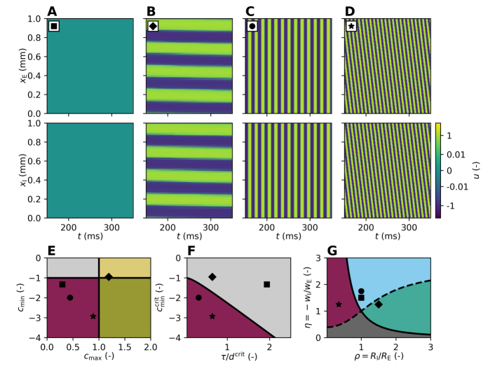
Figure 4: Predictions from linear stability analysis lead to spatiotemporal patterns in simulated network of nonlinear rate neurons. Different parameter combinations, selected according to stability conditions in Table  1, cause pattern formation in rate-neuron network with $\mathrm{tanh}$ gain function. A–D Color-coded activity per neuron over time. Neurons are shown at their position on the ring. E–G Phase diagrams showing conditions and parameter choices indicated by corresponding markers. Purple regions indicate the possibility for wave trains. E Color code indicates stability based on minimum $c_{\mathrm{min}}$ and maximum $c_{\mathrm{max}}$. Gray: Both $c_{\mathrm{min}}$ and $c_{\mathrm{max}}$ stable. Dirty yellow: $c_{\mathrm{max}}$ unstable and $c_{\mathrm{min}}$ stable. Dirty green: $c_{\mathrm{max}}$ unstable and $c_{\mathrm{min}}$ undetermined. Purple: $c_{\mathrm{max}}$ stable and $c_{\mathrm{min}}$ undetermined. A Stable activity (square marker). B Spatial oscillations (diamond marker). C Temporal oscillations (circular marker). D Wave trains (star marker). Parameters: $d$, $R_{\mathrm{E}}$ and $R_{\mathrm{I}}$ as in Fig 1A–D, $w_{\mathrm{E}}=2.73$ in all panels. A $w_{\mathrm{I}}=-4.10$. B $w_{\mathrm{I}}=-3.42$. C $w_{\mathrm{I}}=-4.79$. D $w_{\mathrm{I}}=-3.42$.

Fig 4B illustrates a case where $c_{\mathrm{max}}>1$ causes an instability (diamond marker in panel E). The Hopf bifurcation is remote in the parameter space (panel F) and panel G ensures $k_{\mathrm{max}}>0$. A simulation of the corresponding rate-model network again confirms the predictions and exhibits stationary spatial oscillations (or periodic bumps). The predicted spatial frequency is $k_{\mathrm{max}}/\left(2\pi\right)\approx 3.74\,\mathrm{mm^{-1}}$ and we expect $L\cdot k_{\mathrm{max}}/\left(2\pi\right)$ bumps to emerge. In this finite-sized system with periodic boundary conditions, the bumps are homogeneously distributed across the domain and the wave numbers are integers; here we observe four stripes.

Fig 4C demonstrates temporal oscillations at the parameter combination indicated by the circular marker. We here choose $c_{\mathrm{max}}<1$ and $c_{\mathrm{min}}<-1$ (panel E). The latter condition leads to an entire range of delays that are beyond the bifurcation in panel F; we choose a delay slightly larger than the critical delay, lying to the left of the bifurcation curve. Inferred from panel G, $k_{\mathrm{min}}=0$ and, as expected from the analytical prediction, the oscillations observed in simulations of the rate-neuron network are purely temporal.Based on the temporal eigenvalue with the largest real part, we predict a temporal frequency of $\operatorname{Im}\left[\lambda_{\mathrm{min}}\right]/\left(2\pi\right)\approx 66.68\,\mathrm{Hz}$ which fits well to the simulated oscillation frequency.

Finally, Fig 4D depicts wave trains (denoted by star marker), as predicted by the analytically tractable neural-field model. The instability results from $c_{\mathrm{min}}<c_{\mathrm{min}}^{\mathrm{crit}}$ (panel F) and occurs at $k_{\mathrm{min}}>0$ (panel G) while $c_{\mathrm{max}}$ remains stable (panel E). With a spatial frequency of $k_{\mathrm{min}}/\left(2\pi\right)\approx 3.02\,\mathrm{mm^{-1}}$ and a temporal frequency of $\operatorname{Im}\left[\lambda_{\mathrm{min}}\right]/\left(2\pi\right)\approx 121.01\,\mathrm{Hz}$, the predicted wave-propagation speed is $\operatorname{Im}\left[\lambda_{\mathrm{min}}\right]/\left(k_{\mathrm{min}}\right)\approx 0.04\,\mathrm{mm/ms}$ which is in agreement with the simulated propagation speed of the wave train.

2.5 Linearization of spiking network model

To assess the validity of the predictions obtained from the analytical model for biologically more realistic spiking-neuron networks, we next linearize the dynamics of spiking leaky integrate-and-fire (LIF) neurons and derive a linear system similar to the neural-field model above. The sub-threshold dynamics of a single LIF neuron $i$ with exponentially decaying synaptic currents is described by a set of differential equations for the time evolution of the membrane potential $V_{i}$ and its synaptic current $I_{i}$ as

$$\begin{split}\tau_{\mathrm{m}}\frac{\partial V_{i}}{\mathrm{\partial}t}&=-V_{i}+I_{i}\left(t\right),\\ \tau_{\mathrm{s}}\frac{\partial I}{\mathrm{\partial}t}&=-I_{i}+\tau_{\mathrm{m}}\sum_{j}J_{ij}s_{j}\left(t-d\right),\end{split}$$ (13)

where we follow the convention of [98] (see Eq 62 in Appendix for the relation to physical units). This definition, with both quantities $V_{i}$ and $I_{i}$ having the same unit, conserves the total integrated charge per impulse flowing into the membrane independent of the choice of the synaptic time constant $\tau_{\mathrm{s}}$. The membrane time constant, defined as $\tau_{\mathrm{m}}=R_{\mathrm{m}}C_{\mathrm{m}}$ with membrane resistance $R_{\mathrm{m}}$ and membrane capacitance $C_{\mathrm{m}}$, couples current to the capacitance. We here assume $\tau_{\mathrm{s}}$ to be much smaller than $\tau_{\mathrm{m}}$. The term $s_{j}\left(t\right)=\sum_{k}\delta\left(t-t_{k}^{j}\right)$ denotes a spike train of neuron $j$ which is connected to neuron $i$ with a constant connection strength $J_{ij}$ and transmission delay $d$. Whenever $V_{i}$ reaches the threshold $V_{\theta}$, a spike is emitted and the membrane potential is reset to the resting potential $V_{\mathrm{r}}$ and voltage-clamped for the refractory period $\tau_{\mathrm{ref}}$.

We now assume that, conditioned on the time-dependent spike emission rate $\nu_{i}(t)$ of neuron $i$, spikes are generated independently, thus with Poisson statistics (see, e.g., [64, Section 3.5] for a discussion of this approximation). A neuron then receives a superposition of many such uncorrelated and Poisson-distributed input spikes, so that the probability distribution $p(V,I,t)$ follows a Chapman-Kolmogorov equation. We further assume the amplitudes of postsynaptic potentials to be small, and perform a Kramers-Moyal expansion [99, 100] up to second order, which yields a Fokker-Planck equation for $p(V,I,t)$ in which the first and second infinitesimal moments appear as

$$\begin{split}\mu_{i}\left(t\right)&=\tau_{\mathrm{m}}\sum_{j}J_{ij}\,\nu_{j}\left(t-d\right),\\ \sigma_{i}^{2}\left(t\right)&=\tau_{\mathrm{m}}\sum_{j}J_{ij}^{2}\,\nu_{j}\left(t-d\right).\end{split}{\color[rgb]{1,0,0}}$$ (14)

Here $(\mu_{i},\sigma_{i})$ can be thought of as the first two moments of a Gaussian white noise in the diffusion approximation [101, 68, 99]. This synaptic noise in the input to neuron $i$ depends on the receiving neuron index $i$ and hence on its position. Therefore $\mu_{i}$ and $\sigma_{i}$ also depend on the column $J_{ij}\forall j$ of the connectivity matrix. Such a mean-field approach has been employed previously to study networks of spiking neurons without spatial structure [68, 64, 69, 70]., where $\nu_{j}=\nu$ are identical for all $j$, given by the population-averaged firing rate.

We extend on this approach by assuming that the neurons are placed uniformly with density $\rho_{x}$ on a one-dimensional domain and apply the established procedure to obtain a continuum limit [24]: A volume element $\mathrm{d}x$ of the one-dimensional domain contains the number $\rho_{x}\mathrm{d}x$ of neurons. We further assume that an incoming connection from a neuron at position $y$ to a neuron at position $x$ is drawn independently and identically distributed (i.i.d.) with probability proportional to a spatial profile $\widetilde{p}(x-y)$. Hence the $J_{ij}$ in Eq 14 are i.i.d. Bernoulli variables that take the value $J$ with a probability $\propto\widetilde{p}(x-y)$ and are zero otherwise. The expressions for the first and second infinitesimal moment in Eq 14 of a neuron at position $x$ under expectation of the random connectivity are then

$$\begin{split}\mu\left(x,t\right)&=\tau_{\mathrm{m}}J\int_{-\infty}^{\infty}\,\widetilde{p}\left(x-y\right)\,\nu\left(y,t-d\right)\,\rho_{x}\mathrm{d}y,\\ \sigma^{2}\left(x,t\right)&=\tau_{\mathrm{m}}J^{2}\int_{-\infty}^{\infty}\,\widetilde{p}\left(x-y\right)\,\nu\left(y,t-d\right)\,\rho_{x}\mathrm{d}y.\end{split}$$ (15)

We find it convenient to introduce a normalized profile $p\left(x-y\right)=\frac{\widetilde{p}\left(x-y\right)}{\int\widetilde{p}\left(x^{\prime}\right)\,\mathrm{d}x^{\prime}}$ and to define the number of incoming connections per neuron as $K:=\int\widetilde{p}\left(x^{\prime}\right)\,\rho_{x}\,\mathrm{d}x^{\prime}$.

In the following we formally write down an evolution equation for the rate $\nu\left(x,t\right)$. We denote as $\nu\left(x,t\right)=F\left[\mu\left(x,\circ\right),\,\sigma\left(x,\circ\right)\right]\left(t\right)$ the firing rate of a LIF neuron at position $x$ at time $t$ described by Eq 13 that is driven by a white noise with mean $\mu(x,t)$ and variance $\sigma^{2}\left(x,t\right)$. Clearly, $F\left[\mu,\sigma\right]\left(t\right)$ is a causal functional of its two arguments, which are functions of time (temporal argument denoted by $\circ$). The firing rate of the neuron at time point $t$ only depends on the statistics of its input up to this point, hence on $\mu(x,s)\,\forall s\leq t$ and $\sigma(x,s)\,\forall s\leq t$. Thus we can define this functional as $F\left[\mu\left(\circ\right),\sigma\left(\circ\right))\right]\left(t\right):=\langle\delta\left(t-t_{k}\right)\rangle_{\xi}$, where $t_{k}$ are the time-points of the threshold crossings of Eq 13 under expectation $\left\langle\right\rangle_{\xi}$ over the realization of the white noise $\xi$ with moments Eq 15 and $\delta$ is the Dirac distribution. Since the statistics of the input, the functions $\mu\left(t\right)$ and $\sigma\left(t\right)$, are direct functions of the firing rate $\nu\left(y,t-d\right)$ by Eq 15, the evolution equation takes the form

$$\begin{split}&\nu\left(x,t\right)\\ &=F\left[\tau_{\mathrm{m}}JK\int_{-\infty}^{\infty}\,p\left(x-y\right)\,D_{d}\,\nu\left(y\right)\,\mathrm{d}y,\,\tau_{\mathrm{m}}J^{2}K\int_{-\infty}^{\infty}\,p\left(x-y\right)\,D_{d}\,\nu\left(y\right)\,\mathrm{d}y\right]\left(t\right),\end{split}$$ (16)

where the delay operator $D_{d}$ is defined to act on the second (temporal) argument of the function as $[D_{d}\nu(x)](t)=\nu(x,t-d)$. In principle, the functional $F$ can be computed – for example, by solving the mean first-passage time for the membrane potential $V$ to exceed the threshold. For that purpose, we would drive the neuron with a Gaussian noise with a given, time-dependent statistics parameterized by $\mu$ and $\sigma^{2}$. Powerful numerical methods are available for this purpose [102]. For the purpose of the present work, however, we do not need to determine $F$ in complete generality, since we are only interested in a linear stability analysis of a spatially and temporally homogeneous state $\nu\left(x,t\right)=\nu_{0}$. Hence it is sufficient to study the stability of Eq 16 with respect to spatio-temporal deviations of the form

$$\nu\left(x,t\right)=\nu_{0}+\delta\nu\left(x,t\right),\qquad\delta\nu\ll\nu_{0}.$$ (17)

Linearizing Eq 16 we obtain (by a functional Taylor expansion or Volterra expansion to first order)

$$\begin{split}&\nu_{0}+\delta\nu\left(x,t\right)\\ &=F\left[\mu_{0},\sigma_{0}^{2}\right]+\int_{-\infty}^{\infty}\,p\left(x-y\right)\,\int_{-\infty}^{t}\,h_{\nu}(\mu_{0},\sigma_{0},t-s)\,\delta\nu\left(y,s-d\right)\,\mathrm{d}s\,\mathrm{d}y+\mathcal{O}\left(\delta\nu^{2}\right),\\ &\text{with }h_{\nu}(\mu_{0},\sigma_{0},t-s)=\tau_{\mathrm{m}}JK\,\frac{\delta F\left[\mu_{0},\sigma_{0}^{2}\right]\left(t\right)}{\delta\mu\left(s\right)}+\tau_{\mathrm{m}}J^{2}K\,\frac{\delta F\left[\mu_{0},\sigma_{0}^{2}\right]\left(t\right)}{\delta\sigma^{2}\left(s\right)},\end{split}$$ (18)

where we introduce the short hand $\mu_{0}=\tau_{\mathrm{m}}JK\nu_{0}$ and $\sigma_{0}^{2}=\tau_{\mathrm{m}}J^{2}K\nu_{0}$. With $\nu_{0}=F\left[\mu_{0},\sigma_{0}^{2}\right]$ the first line of Eq 18 cancels the corresponding term on the left hand side and we obtain a linear convolution equation for the rate deflection $\delta\nu$, whose spectral properties we need to analyze. The stationary firing rate $\nu_{0}$ can be determined self-consistently from this condition (see Eq 52 in Appendix). The functional derivatives

$$\frac{\delta F\left[\mu_{0},\sigma_{0}^{2}\right]\left(t\right)}{\delta\mu\left(s\right)} \equiv\lim_{\epsilon\to 0}\,\frac{1}{\epsilon}\big{(}F\left[\mu_{0}+\epsilon\,\delta\left(\circ-s\right),\,\sigma_{0}^{2}\right]\left(t\right)-F\left[\mu_{0},\sigma_{0}^{2}\right]\left(t\right)\big{)},$$

(and analogous for $\delta F/\delta\sigma^{2}$) are, by the right hand side of this definition, the responses of the system with respect to an impulse-like perturbation of $\mu$ and $\sigma^{2}$, respectively. We denote these as

$$\begin{split}h_{\mu}\left(t-s\right)&\equiv\frac{\delta F\left[\mu_{0},\sigma_{0}^{2}\right]\left(t\right)}{\delta\mu\left(s\right)},\\ h_{\sigma^{2}}\left(t-s\right)&\equiv\frac{\delta F\left[\mu_{0},\sigma_{0}^{2}\right]\left(t\right)}{\delta\sigma^{2}\left(s\right)},\end{split}$$ (19)

which are causal functions of $t-s$ only, since we linearize around a time-translation invariant state and causality clearly requires both kernels to vanish for $s>t$. These functions can analytically be computed in the Fourier domain for LIF models with instantaneous synapses [64, 103], for fast colored noise [104], and in the adiabatic limit for slow synapses [105, 106]; see 4.4 for details. The form of the response kernels Eq 19 is given in Eqs 53–55 in Appendix. These expressions are obtained by a perturbative calculation on the level of the Fokker-Planck equation that is correct to leading order in $\mathcal{O}(\sqrt{\tau_{s}/\tau_{m}})$ [104], thus constitude good approximations for sufficiently short synaptic time constants. With this notation, the linearized dynamics Eq 18 obeys a convolution equation in space and time

$$\delta\nu\left(x,t\right)=\int_{-\infty}^{\infty}\,p\left(x-y\right)\,\int_{-\infty}^{t}\,h_{\nu}(t-s)\,\delta\nu(y,s-d)\,\mathrm{d}y\,\mathrm{d}s,$$ (20)

whose stability properties can be analyzed in Fourier domain by standard methods.

In the following section we will ignore the kernel $h_{\sigma^{2}}$, because its contribution is usually small [104]. Eq 20 provides a linearized system for the spiking model that is continuous in space and time and enables a direct comparison with the neural-field model in the following section.

2.6 Comparison of neural-field and spiking models

The linearization of the LIF model presented in the preceding section is the analogue to taking the derivative $\psi^{\prime}$ of the gain function in the linear stability analysis of the neural-field model in Section 2.1. By the assumption of conditional independence of spike trains given their firings rate, we achieve that the state of the spiking network is described by the time-dependent firing rate profile $\nu(x,t)$. Its temporal evolution follows Eq 16. This function therefore conceptually plays the same role as $u(x,t)$ in the neural-field model. Therefore the results for the neural field model carry over to the spiking case. To expose the similarities between the linearized systems of the spiking model and the neural-field model, we may bring the equations for the deviation from baseline activity

$$\delta o(x,t) =\begin{cases}\delta u(x,t)&\text{neural field}\\ \delta\nu(x,t)&\text{spiking}\end{cases}$$ (21)

to the form of the convolution equation

$$\begin{split}\delta o(x,t)&=\left[h\ast\delta i\right](x,t)\\ \delta i\left(x,t\right)&=\int_{-\infty}^{\infty}p\left(x-y\right)\,\delta o\left(y,t-d\right)\,\mathrm{d}y,\end{split}$$ (22)

where the only difference is the convolution kernel relating the deviation from the input $\delta i$ to those of the output $\delta o$ defined as

$$h(t) :=\begin{cases}h^{\mathrm{nf}}(t):=\Theta(t)\,\frac{w}{\tau}\,\mathrm{e}^{-\frac{t}{\tau}}&\text{neural field}\\ h^{\mathrm{s}}(t):=\tau_{\mathrm{m}}JK\,h_{\mu}(t)&\text{spiking.}\end{cases}$$ (23)

The kernel on the first line is the fundamental solution (Green’s function) of the linear differential operator appearing on the left hand side of Eq 1, including the coupling weight $w$. As a consequence, the characteristic equations for both models result from the Fourier-Laplace ansatz $\delta o\left(x,t\right)=\mathrm{e}^{\mathrm{i}kx}\mathrm{e}^{\lambda t}$ which relates the eigenvalues $\lambda$ to the wave number $k$ as

$$H\left(\lambda\right)\cdot\mathrm{e}^{-\lambda d}\cdot\widehat{p}\left(k\right)=1.$$ (24)

The effective transfer function $H$ describes the linear input-output relationship Eq 22 in the Laplace domain. It is obtained as the Laplace transform of Eq 23 of the respective functions for the spiking model $h^{\mathrm{s}}\left(t\right)$ and for the neural-field model $h^{\mathrm{nf}}$$\left(t\right)$. As a result we obtain the transfer function for the neural-field model

$$H^{\mathrm{nf}}\left(\lambda\right) =\frac{1}{1+\lambda\tau}w.$$ (25)

The corresponding expression for the effective spiking transfer function $H^{\mathrm{s}}\left(\lambda\right)$ results from Eqs 53-55 in Appendix.

2.6.1 Parameter mapping

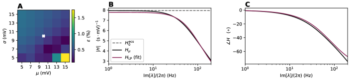
Figure 5: Transfer function of spiking neuron model and its approximation. A Fitting error of the low-pass filter approximation of the transfer function for LIF neurons derived in [104] over $\mu$ and $\sigma$ (given relative to the reset potential). The fitting error $\epsilon=\sqrt{\epsilon_{\tau}^{2}+\epsilon_{H_{0}}^{2}}$ is color-coded. B Amplitude of the transfer function and approximation (legend). Dashed line illustrates $H_{0}$ following from the analytically-determined effective coupling strength (see Eq 56 in Appendix). C Phase. The white cross in panel A indicates the working point $\left(\mu,\sigma\right)$ selected for the transfer function shown in panels B and C and used in the simulations throughout the study.

So far the stability analysis shows that the characteristic equations for both the neural-field and the spiking model have the same form Eq 24 given a proper definition of the respective transfer functions. The transfer function characterizes the transmission of a small fluctuation in the input to the output of the neuron model. Because the transfer functions differ between the two models, it is a priori unclear whether their characteristic equations have qualitatively similar solutions. To provide evidence that this is indeed the case, in the following we devise a procedure that identifies solutions of the characteristic equations in Eq 24 for the rate model and the spiking model, and develop a practical method to obtain one solution from the other.

To this end we use that the transfer function of the LIF model in the fluctuation-driven regime investigated here can be approximated by a first order low-pass (LP) filter [103, 107, 97] (see in particular [107, Fig 1]) with effective parameters $H_{0}$ and $\tau$

$$H_{\mu}\left(\lambda\right)\approx H_{\mathrm{LP}}\left(\lambda\right)=\frac{H_{0}}{1+\lambda\tau},$$ (26)

where $H_{\mu}$ is the Fourier transform of $h_{\mu}$, defined in Eq 19. This simplified transfer function is similar to the the transfer function Eq 25 of the neural-field model, and thereby relates the phenomenological parameters $w$ and $\tau$ of the neural-field model to the biophysically motivated parameters of the spiking model.

We perform a least squares fit between $H_{\mathrm{LP}}\left(\lambda\right)$ and $H_{\mu}\left(\lambda\right)$ to obtain the values for the parameters $\tau$ and $H_{0}$. According to Eq 23, $H_{0}$ directly relates to $w$ as

$$w=H_{0}\tau_{\mathrm{m}}JK,$$ (27)

which follows by noting that $\int h_{\mu}(t)=H_{\mu}(0)\approx H_{0}$. The goodness of the fit of this transfer function to the first-order low-pass filter depends on the mean $\mu$ and variance $\sigma$ of the synaptic input, as shown in Fig 5A. The color-coded error of the fit combines the relative errors from both fitting parameters: $\epsilon=\sqrt{\epsilon_{\tau}^{2}+\epsilon_{H_{0}}^{2}}$. For the majority of working points $\left(\mu,\sigma\right)$ the error is $<1\%$ but the relative errors increase abruptly towards the mean-driven regime. In this regime input fluctuations are small and the mean input predominantly drives the membrane potential towards threshold, so that the model fires regularly and the transfer function exhibits a peak close to the firing frequency [103, 107]. We here fix the working point to the parameters indicated by the white cross (see Eq 61 in Appendix) for all populations, resulting in a common effective time constant $\tau$. Here, we obtain a time constant $\tau=1.94\,\mathrm{ms}$ which thus lies in between the synaptic time constant, $\tau_{\mathrm{s}}=0.5\,\mathrm{ms}$, and the membrane time constant, $\tau_{\mathrm{m}}=5\,\mathrm{ms}$, of the LIF neuron model. For these parameters, Fig 5B shows the amplitude and Fig 5C the phase of the original transfer function $H_{\mu}\left(\lambda\right)$ in black and the fitted transfer function $H_{\mathrm{LP}}\left(\lambda\right)$ in purple. The dashed gray line denotes $H_{0}$ obtained by computing the effective coupling strength from linear response theory, $H_{0}^{\mathrm{ecs}}$, as a reference (see Eq 56 in Appendix).

2.6.2 Linear interpolation between the transfer functions

Evaluating the characteristic equation for the neural-field model yields an exact solution for each branch of the Lambert W function, given by Eq 7. For this model we already established that the principle branch is the most unstable one. An equivalent condition is not known for the general response kernel of the LIF neuron. To asses whether we may transfer the result for the neural-field model to the spiking case, we investigate the correspondence between the two characteristic equations that are both of the form Eq 24 but with different transfer functions. For this purpose, we define an effective transfer function

$$H_{\alpha}\left(\lambda\right)=\alpha H^{\mathrm{s}}\left(\lambda\right)+\left(1-\alpha\right)H^{\mathrm{nf}}\left(\lambda\right),$$ (28)

with the parameter $\alpha$ that linearly interpolates between the effective transfer functions of the spiking and the neural-field model: $H_{\alpha=0}\left(\lambda\right)=H^{\mathrm{nf}}$$\left(\lambda\right)$ and $H_{\alpha=1}\left(\lambda\right)=H^{\mathrm{s}}$$\left(\lambda\right)$. Fig 6 illustrates two different ways for solving the combined characteristic equation

$$H_{\alpha}\left(\lambda\right)\cdot\mathrm{e}^{-\lambda d}\cdot\widehat{p}\left(k\right)=1.$$ (29)

The first results from computing the derivative $\partial\lambda/\partial\alpha$ (see Eqs 57-59 in Appendix) from the combined characteristic equation and integrating numerically with the exact solution of the neural-field model at $\alpha=0$ for each branch $b$ as initial condition:

$$\lambda\left(\alpha\right)=\int_{0}^{\alpha}\frac{\mathrm{\partial}\lambda}{\partial\alpha^{{}^{\prime}}}\,\mathrm{d}\alpha^{{}^{\prime}},\qquad\lambda\left(0\right)=\lambda_{b}$$ (30)

with

$$\frac{\mathrm{\partial}\lambda}{\mathrm{\partial}\alpha}=-\frac{H^{\mathrm{s}}\left(\lambda\right)-H^{\mathrm{nf}}\left(\lambda\right)}{\alpha\frac{\partial H^{\mathrm{s}}\left(\lambda\right)}{\partial\lambda}+\left(1-\alpha\right)\frac{\partial H^{\mathrm{nf}}\left(\lambda\right)}{\partial\lambda}-d\cdot H_{\alpha}\left(\lambda\right)}.$$ (31)

Figure 6: Linear interpolation between neural-field $\left(\alpha=0\right)$ and spiking $\left(\alpha=1\right)$ model for eigenvalue close to bifurcation. A Real and B imaginary part of the eigenvalue $\lambda$ as a function of the linear interpolation parameter $\alpha$ for the characteristic equation in Eq 29. The solution at $\alpha=0$ for the neural-field model is exact. C Real and D imaginary part of the eigenvalues (same units but different scaling as in A and B) with analytically exact solution (by Lambert W function, $\alpha=0$) as functions of the wave number $k$. Different branches $b$ are color-coded (legend); $b=0$ corresponds to the principal branch with the maximum real eigenvalue (gray cross). Circular markers denote the linear interpolation according to the numerical integration of Eq 30. Dashed line segments for the linear interpolation are obtained by solving the characteristic equation Eq 29 numerically. Both are evaluated at the same values for $\alpha$. Parameters: $d=1.5\,\mathrm{ms}$, $R_{\mathrm{E}}=0.2\,\mathrm{mm}$, $R_{\mathrm{I}}=0.07\,\mathrm{mm}$, $g=5.$

The spatial profile only enters the initial condition, and the derivative Eq 31 is independent of the wave number $k$.

As an alternative approach, we directly solve the combined characteristic equation Eq 29 numerically with the known initial condition. Fig 6A and B indicate that only the principle branch ($b=0$) becomes positive while the other branches remain stable. The branches come in complex conjugate pairs. For the numerical solution of the characteristic equation, we fix the wave number to the value of $k$ that corresponds to the maximum real eigenvalue.

The analysis shows that we may ignore the danger of branch crossing since different branches remain clearly separated in Fig 6A and B. In addition, the eigenvalue on the principle branch is mostly independent of $\alpha$, even if the system is close to the bifurcation (when the real part of $\lambda_{0}$ is close to zero). Thus for all values of $\alpha$ we expect qualitatively similar bifurcations, including $\alpha=1$. This justification transfers the rigorous results from the bifurcation analysis of the neural-field model in Section 2.2 and Section 2.3, and corresponding effective parameters, to the spiking model.

2.7 Validation by simulation of spiking neural network

The Introduction illustrates spatiotemporal patterns emerging in a spiking network simulation in Fig 1 and the subsequent sections derive a theory describing the mechanisms underlying such patterns. Finally, the parameter mapping between the spiking and the neural-field model explains the origin of the spike patterns by transferring the conditions found for the abstract neural-field model in Section 2.2 and Section 2.3 to the spiking case. This section validates that the correspondence between network parameters in the two models is not incidental but covers the full phase diagram.

In the following, we simulate a network with the same neural populations and spatial connectivity used in the nonlinear rate-network in Fig 4, but replace the rate-model neurons by spiking neurons, and map the parameters as described in Section 2.6.1. The network model characterizes all neurons by the same working point (see Eq 61 in Appendix), which means that the connectivity matrix for the excitatory-inhibitory network has equal rows; entries in Eq 4 depend on the presynaptic population alone. Therefore the relative in-degree $\gamma=K_{\mathrm{I}}/K_{\mathrm{E}}$ and the relative synaptic strength $g=-J_{\mathrm{I}}/J_{\mathrm{E}}$ parametrize the spiking-network connectivity matrix as

$$M\left(r\right)=\tau_{m}J_{\mathrm{E}}K_{\mathrm{E}}\,\left(\begin{array}[]{cc}p_{\mathrm{E}}\left(r\right)&-\gamma g\,p_{\mathrm{I}}\left(r\right)\\ p_{\mathrm{E}}\left(r\right)&-\gamma g\,p_{\mathrm{I}}\left(r\right)\end{array}\right).$$ (32)

The rightmost panels of Fig 7A–C show the same simulation results as Fig 1B–D; likewise the panels of Fig 1 have parameters that correspond to those of the rate-neuron network in Fig 4. The different patterns in Fig 1B–D emerge by gradually shifting a single network parameter that switches the system from a stable state (white filled markers in Fig 7D and E), across intermediate states (gray-scale filled markers) to the final states where stability is lost and the patterns have formed (black filled markers). Arrows visualize the sequences in the phase diagrams Fig 7D and E and the markers reappear in the upper left corners of the corresponding raster plots in Fig 7A–C.

The sequence of panels in Fig 7A illustrates a gradual transition from a stable (AI) state to spatial oscillations attained by increasing the amplitudes of excitatory postsynaptic current (PSC) amplitudes $J_{\mathrm{E}}^{{}^{\prime}}$ in the network. With $J^{{}^{\prime}}$ we denote the weight as a jump in current while $J$ denotes a jump in voltage in the physical sense, and the relationship is: $J^{{}^{\prime}}=C_{\mathrm{m}}J/\tau_{s}$ (see Eq 62 in Appendix). The parameter variation thus homogeneously scales the effective profile $c$ but preserves the shape of the reduced profile $\widetilde{c}$ (fixed position of diamond marker in panel F). Simultaneously an increasing rate of the external Poisson input compensates for the reduced PSC amplitudes to maintain the fixed working point $\left(\mu,\sigma\right)$ of the neurons (see Eq 61 in Appendix). Diamond markers in Fig 7D show that along its path the system crosses the critical value $c_{\mathrm{max}}=1$, while $c_{\mathrm{min}}>c_{\mathrm{min}}^{\mathrm{crit}}(\tau/d^{\mathrm{crit}})$ stays in the stable regime, as shown in panel E. However, even for $c_{\mathrm{max}}\lesssim 1$ (for $J_{E}^{{}^{\prime}}=60\,\mathrm{pA}$) the network activity already exhibits weak spatial oscillations.

Choosing the synaptic delay $d$ as a bifurcation parameter highlights the onset of temporal oscillations for the case $k=0$ (panel B sequence, circular markers) and spatiotemporal oscillations for the case $k>0$ (sequence in Fig 7C, star markers). In contrast to the case of purely spatial waves in panel A, the procedure preserves the effective spatial profile (fixed positions in panels D and F) and the system crosses the transition curve in panel E due to increasing delay alone, thus decreasing the ratio $\tau/d$.

Fig 7C illustrates the gradual transition to wave trains, where $c_{\mathrm{max}}$ remains in the theoretically stable regime at all times, but is close to the critical value of $1$ (see the star marker in panel D). As a result, we observe spatial oscillations with a spatial frequency given by $k_{\mathrm{max}}$ before and even after the Hopf bifurcation. For delays longer than the critical delay, mixed states occur in which different instabilities due to $c_{\mathrm{max}}$ and $c_{\mathrm{min}}$ compete. The different spatial frequencies $k_{\mathrm{max}}/\left(2\pi\right)$ and $k_{\mathrm{min}}/\left(2\pi\right)$ become visible. For delay values well past the bifurcation, this mixed state is lost resulting in a dependency only on $c_{\mathrm{min}}$ and wave trains with a spatial frequency that depends on $k_{\mathrm{min}}$.

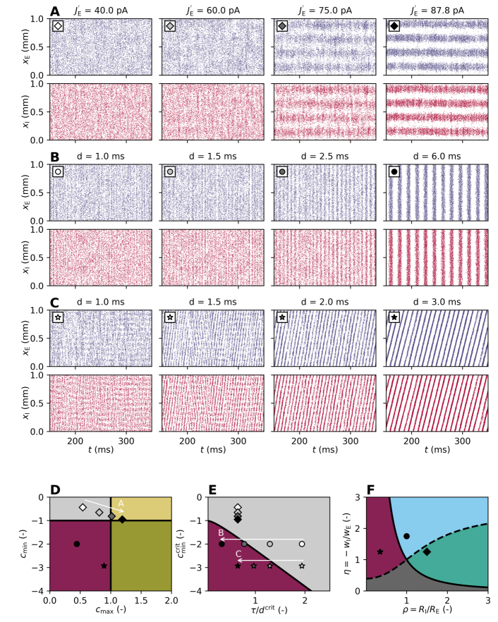
Figure 7: Transitions from theoretically stable states to spatiotemporal patterns in spiking network simulation. A–C Spike rasters showing transition to network states in Fig 1B–D (same markers, same parameter combinations). The changed parameter value is given on top of each raster plot. A Increasing recurrent weight $J_{\mathrm{E}}^{{}^{\prime}}$ leads to onset of spatial oscillations. B Increasing synaptic delay $d$ leads to onset of temporal oscillations at $k=0$. C Increasing delay $d$ leads to onset of temporal oscillations at $k>0$, i.e., wave trains. D–E Gray shaded markers and white arrows labeled according to respective panel A-C in phase diagrams indicate sequences of parameter combinations and breakdown of stability at $c_{\mathrm{max}}=1$ or at $c_{\mathrm{min}}=c_{\mathrm{min}}^{\mathrm{crit}}$. For each sequence in panels A–C, delay $d$, excitatory profile width $R_{\mathrm{E}}$, inhibitory profile width $R_{\mathrm{I}}$, and the relative synaptic strength $g$ correspond to the values given in Fig 1B–D with corresponding markers.

3 Discussion

The present study employs mean-field theory [64] to rigorously map a spiking network model of leaky integrate-and-fire (LIF) neurons with constant transmission delay to a neural-field model. We use a conceptually similar linearization as Kriener et al. [92] combined with an analytical expressions for the transfer function in the presence of colored synaptic noise [104]. The insight that this transfer function in the fluctuation-driven regime resembles the one of a simple first-order low-pass filter facilitates the parameter mapping between the two models. The resulting analytically tractable effective rate model depends on the dynamical working point of the spiking network that is characterized by both the mean and the variance of the synaptic input. By means of bifurcation theory, in particular linear Turing instability analysis [29, 45, 44], we investigate the origin of spatiotemporal patterns such as temporal and spatial oscillations and in particular wave trains emerging in spiking activity. The mechanism underlying these waves encompasses delay-induced fast global oscillations, as described by Brunel and Hakim [64], with spatial oscillations due to a distance-dependent effective connectivity profile. We derive analytical conditions for pattern formation that are exclusively based on general characteristics of the effective connectivity profile and the delay. The profile is split into a static weight that is either excitatory or inhibitory for a given neural population, and a spatial modulation that can be interpreted as a distance-dependent connection probability. Given the biological constraint that connection probabilities depend on distance but weights do not, wave trains cannot occur in a single homogeneous population irrespective of the shape of distance-dependent connection probability. Only the effective connectivity profile of two populations (excitatory and inhibitory), permits solutions where a mode with finite non-zero wave number is the most unstable one, a prerequisite for the emergence of nontrivial spatial patterns such as wave trains. We therefore establish a relation between the anatomically measurable connectivity structure and observable patterns in spiking activity. The predictions of the analytically tractable neural-field model are validated by means of simulations of nonlinear rate-unit networks [108] and of networks composed of LIF-model neurons, both using the same simulation framework [109]. In our experience, the ability to switch from a model class with continuous real-valued interaction to a model class with pulse-coupling by changing a few lines in the formal high-level model description increases the efficiency and reliability of the research.

The presented mathematical correspondence between these a priori distinct classes of models for neural activity has several implications. First, as demonstrated by the application in the current work, it facilitates the transfer of results from the well-studied domain of neural-field models to spiking models. The insight thus allows the community to arrive at a coherent view of network phenomena that appear robustly and independently of the chosen model. Second, the quantitative mapping of the spiking model to an effective rate model in particular reduces the parameters of the former to the set of fewer parameters of the latter; single-neuron and network parameters are reduced to just a weight and a time constant. This dimensionality reduction of the parameter space conversely implies that entire manifolds of spiking models are equivalent with respect to their bifurcations. Such a reduction supports systematic data integration: Assume a researcher wants to construct a spiking model that reproduces a certain spatiotemporal pattern. The presented expressions permit the scientist to restrict further investigations to the manifold in parameter space in line with these observations. Variations of parameters within this manifold may lead to phenomena beyond the predictions of the initial bifurcation analysis. Additional constraints, such as firing rates, degree of irregularity, or correlations, can then further reduce the set of admissible parameters.

To keep the focus on the transferability of results from a neural-field to a spiking model, the present study restricts the analysis to a rather simple network model. In many cases, extensions to more realistic settings are straight forward. As an example, we perform our analysis in one-dimensional space. In two dimensions, the wave number becomes a vector and bifurcations to periodic patterns in time and space can be constructed (see [28, Section 8.4] and [29]). Likewise, we restricted ourselves to a constant synaptic delay like Roxin et al. [42, 51] because it enables a separation of a spatial component, the shape of the spatial profile, and a temporal component, the delay. A natural next step is the inclusion of an axonal distance-dependent delay term as for instance in [40] to study the interplay of both delay contributions [58]. For simplification, we use here a boxcar-shaped spatial connectivity profile in the demonstrated application of our approach. For the emergence of spatiotemporal patterns, however, the same conditions on the connectivity structure and the delays hold for more realistic exponentially decaying or Gaussian-shaped profiles [20, 21, 22]. If the spatial connectivity profiles are monotonically decaying in the Fourier domain (as it is the case for exponential or Gaussian shapes), the Fourier transform of the effective profile of a network composed of an excitatory and an inhibitory population exhibits at most one zero-crossing. Either the minimum or the maximum are attained at a non-zero and finite wave number $k$, but not both. With a cosine-shaped effective profile, only a single wave number dominates by construction [42, 51]. Here, we decided for the boxcar shape because of its oscillating Fourier transform that allows us to study competition between two spatial frequencies corresponding to the two extrema.

Similar to our approach, previous neural-field studies describe the spatial connectivity profile as a symmetric probability density function (see, for example, [49]). For our aim, to establish a link to networks of discrete neurons, the interpretation as a connection probability and the separation from a weight are a crucial addition. This assumption enables us to distinguish between different neural populations, to analyze the shape of the profile based on parameters for the excitatory and the inhibitory contribution, and to introduce biophysically motivated parameters for the synaptic strength. Starting directly with an effective profile that includes both, excitation and inhibition, such as (inverse) Mexican hat connectivity, is mathematically equivalent and a common approach in the neural-fields literature [40, 53, 29, 42]. But it neglects the biological separation of neurons into excitatory and inhibitory populations according to their effect on postsynaptic targets (Dale’s law [110]) and their different spatial reach of connectivity [111]. A result of this simplification, these models can produce waves even with a single homogeneous population [42, 43, 44], while with homogeneous stationary external drive we show that at least two populations are required.

Local excitation and distant inhibition are often used to support stationary patterns such as bumps, while local inhibition and distant excitation are associated with non-stationary patterns such as traveling waves [112, 28, 40]. For sufficiently long synaptic delays, we also observe wave trains with local inhibition and distant excitation, as often observed in cortex [111]. However, we show that the reason for this is the specific shape of the effective spatial profile, and not only the spatial reach itself. Our argumentation is therefore in line with Hutt et al. [48, 54] who demonstrate that wave instabilities can even occur with local excitation and distant inhibition for specific spatial interactions. The spatial connectivity structure and related possible activity states are in addition important factors for computational performance or function of model networks [113, 90].

In Section 2.4, we compute the spatial and temporal oscillation frequencies as well as the wave-propagation speed. Such quantities are directly comparable with experimental measurements. The conduction speed in unmyelinated fibers is in the $0.1\,\mathrm{mm/ms}$ range and the propagation speed of mesoscopic waves is of similar order of magnitude [114, 115]. Our prediction based on the current choice of model parameters is with $0.04\,\mathrm{mm/ms}$ in the same order of magnitude.

The parameter mapping between a neural-field and a spiking model in this study relies on the insight that the transfer function of the LIF neuron in the fluctuation-driven regime resembles the one of a simple first-order low-pass filter. Since this approximation not only holds for LIF neurons, but also for other spiking neuron models, our results are transferable. A further candidate model with this property is the exponential integrate-and-fire model [116]. Other examples include Nordlie et al. [117] who characterize the firing-rate responses of LIF neurons with strong alpha-shaped synaptic currents and similarly Heiberg et al. [118] for a LIF neuron model with conductance based synapses and potassium-mediated afterhyperpolarization currents proposed previously [119].

In the literature, the time constant of neural-field models is often associated with the membrane or the synaptic time constant [79, 33, 90]. Here, we observe that the time constant of the neural-field model derived from the network of spiking neurons falls in between the two. In line with [120, 117], we suggest to reconsider the meaning of the time constant in neural-field models.

A limitation of the approach employed here is that the linear theory is only exact at the onset of waves. Beyond the bifurcation, it is possible that nonlinearities in the spiking model govern the dynamics and lead to different prevailing wave numbers or wave frequencies than predicted. Roxin et al. [51] report that the stability of traveling waves depends crucially on the nonlinearity. Nevertheless they do not observe traveling waves in their spiking-network simulations. In the present work, however, we identify biophysically motivated neuron and network parameters that allow wave trains to establish in a spiking network. Still, we had to increase the delay beyond the predicted bifurcation point to obtain a stable wave pattern.

Furthermore, the theory underlying the mapping of the spiking network to the neural-field model is based on the diffusion approximation and therefore only applicable for sufficiently small synaptic weights. Widely distributed synaptic weights, for example, may lead to larger deviations. We here primarily target a wave-generating mechanism for cortical networks. Since in other brain regions involved neuron types, connectivity structures and input characteristics are different, other mechanisms for pattern formation not covered in this work need to be taken into account [3].

The working-point dependence of the neural-field models derived here offers a new interpretation of propagating activity measured in vivo [12, 8]. Even if the anatomical connectivity remains unchanged during a period of observation, the stability of the neural system can be temporarily altered due to changes in activity. The transfer function of a LIF neuron depends on the mean and the variance of its input, and we have shown that stability is related to its parametrization. In particular, local changes of activity, for example due to a spatially confined external input, can affect stability and hence influence whether a signal remains rather local or travels across the cortical surface. That means, we would relate the tendency of a neural network to exhibit spatiotemporal patterns not only to its connectivity, but also to its activity state that can change over time.

4 Appendix

4.1 Linear stability analysis

4.1.1 Derivation of the characteristic equation

With the Fourier-Laplace ansatz $u\left(x,t\right)=e^{\mathrm{i}kx}\mathrm{e}^{\lambda t}$ for the integro-differential equation in Eq 1 linearized around $u_{0}$ and the choice to set the slope of the gain function to unity, the characteristic equation in Eq 3 results from

$$\begin{split}\tau\lambda\,\mathrm{e}^{ikx}\mathrm{e}^{\lambda t}&=-\mathrm{e}^{ikx}\mathrm{e}^{\lambda t}+\int_{-\infty}^{\infty}wp\left(x-y\right)\mathrm{e}^{iky}\mathrm{e}^{\lambda\left(t-d\right)}\,\mathrm{d}y\\ \tau\lambda&=-1+w\mathrm{e}^{-\lambda d}\int_{-\infty}^{\infty}p\left(x-y\right)\mathrm{e}^{-ik\left(x-y\right)}\,\mathrm{d}y\\ &=-1-w\mathrm{e}^{-\lambda d}\int_{\infty}^{-\infty}p\left(r\right)\mathrm{e}^{-ikr}\,\mathrm{d}r,\qquad r=x-y\\ &=-1+w\mathrm{e}^{-\lambda d}\underbrace{\int_{-\infty}^{\infty}p\left(r\right)\mathrm{e}^{-ikr}\,\mathrm{d}r}_{\equiv\widehat{p}\left(k\right)}.\end{split}$$ (33)

In the last row, we recognize the Fourier transform $\widehat{p}$ of the spatial profile $p$.

4.1.2 Effective connectivity profile for two populations

While the connectivity $m$ is a scalar in the one-population model, it is a matrix $M$ in the case of two populations (given in Eq 4). The ansatz for deriving the characteristic equation in the latter case reads $\delta u\left(x,t\right)=v\mathrm{e}^{\mathrm{i}kx}\mathrm{e}^{\lambda t}$, with $v$ denoting a vector of constants. This leads to the auxiliary eigenvalue problem

$$c\left(k\right)\,v=\widehat{M}\left(k\right)\,v,$$ (34)

where $c$ denotes an eigenvalue and $\widehat{M}$ is an auxiliary matrix containing the Fourier transforms of the entries of $M$:

$$\widehat{M}\left(k\right)=\left(\begin{array}[]{cc}w_{\mathrm{EE}}\,\widehat{p}_{\mathrm{EE}}\left(k\right)&w_{\mathrm{EI}}\,\widehat{p}_{\mathrm{EI}}\left(k\right)\\ w_{\mathrm{IE}}\,\widehat{p}_{\mathrm{IE}}\left(k\right)&w_{\mathrm{II}}\,\widehat{p}_{\mathrm{II}}\left(k\right)\end{array}\right).$$ (35)

Eq 34 possesses a nontrivial solution $v$ if and only if $\det\left(\widehat{M}\left(k\right)-c\left(k\right)\mathbbm{1}\right)=0$. Eq 5 explicitly states the two eigenvalues $c_{1,2}$ solving this equation. These eigenvalues constitute the effective profile in the characteristic equation in Eq 3 that hence holds also for the two-population case.

4.1.3 Largest real part on principle branch of Lambert W function

The function $x\left(W\right)=W\,\mathrm{e}^{W}$ has a minimum at $W=-1$, no real solution for $x<-\mathrm{e}^{-1}$, a single solution for $x>0$, and two solutions for $x\in[-e^{-1},0)$. Typically, the term ‘principal branch’ of the Lambert W function with branch number $b=0$ refers to the real branch defined on the interval $[-e^{-1},\infty)$, where for negative arguments the larger solution is considered. Here we extend the definition to the whole real line by the complex branch with maximal real part and positive imaginary part on $(-\infty,-e^{-1})$.

We demonstrate that the branch of the Lambert W function with the largest real part is the principal branch. Considering only real-valued arguments $x\in\mathbb{R}$, we write $W\left(x\right)=\left|W\left(x\right)\right|\mathrm{e}^{i\varphi}=\alpha+i\beta$ and

$$W\left(x\right)\mathrm{e}^{W\left(x\right)} =\left|W\left(x\right)\right|\,\mathrm{e}^{\alpha}\,\mathrm{e}^{i\left(\varphi+\beta\right)}=x\in\mathbb{R}$$ (36)

$$\rightarrow\mathrm{e}^{i(\varphi+\beta)} =\pm 1,$$ (37)

where $\varphi\in\left[-\pi,\pi\right]$ is the principal value. We index the branches by $q\in\mathbb{Z}$ according to the number of half-cycles of the exponential in Eq 37: $\varphi+\beta=q\cdot\pi$. The branch number is equal to $b=\left\lfloor\frac{q}{2}\right\rfloor$ with $\left\lfloor\cdot\right\rfloor$ denoting the floor function. The principle branch is therefore given by the index $q=0$ for $x\geq 0$ and by $q=1$ for $x<0.$

Taking the absolute square of Eq 36 yields the real equation

$$x^{2}\,\mathrm{e}^{-2\alpha}=\alpha^{2}+\beta^{2}.$$ (38)

Without loss of generality we may assume $\beta\geq 0$; this is certainly true for the real solutions with $\beta=0$ and it also holds for one of the complex solutions for any complex pair. Complex solutions come in conjugate pairs due to the symmetry $(\varphi,\beta)\to(-\varphi,-\beta)$ exhibited by Eq 37 and Eq 38. Since each member of a pair has by definition the same real part, it is sufficient to consider only the member with positive imaginary part $\beta>0$.

To prove that the real part $\alpha$ of $W$ is maximal for $b=0$, we show that $\alpha$ is a decreasing function of $\beta$ along the solutions of Eq 36. Investigating the intersections of the left-hand side and the right-hand side of Eq 38 as a function of $\alpha$ illustrates how increasing the imaginary part $\beta$ affects the real part $\alpha$. The left-hand side is a decaying function of $\alpha$ with an intercept of $x^{2}$. The right-hand-side is a parabola with an offset of $\beta^{2}$.

For $x\in(-\infty,-e^{-1})\cup\left[0,\infty\right)$, an intersection occurs either at a positive real part $\alpha\geq 0$ if $x^{2}\geq\beta^{2}$, or at a negative real part $\alpha<0$ if $x^{2}<\beta^{2}$. Increasing $\beta$ moves the parabola upwards and therefore the intersection to the left, meaning that $\alpha$ decreases with increasing $\beta$.

For $x\in[-e^{-1},0)$, we distinguish the cases $\beta=0$ and $\beta>0$ which both have only solutions with $\alpha<0$. First, the two real solutions ($q=\pm 1$) existing in this interval correspond to two simultaneously occurring intersections; in addition a third intersection is created by the squaring Eq 38 but it is not an actual solution of Eq 36. The intersection at the larger real part per definition corresponds to the principal branch with index $q=1$. Second, the complex solutions are indexed by odd numbers $q$ with $\left|q\right|>1$. Taking into account the interval where $\varphi$ is defined, the imaginary part is bounded from below such that $\beta\geq 2\pi$ for non-principal branches. Analogous to the previously discussed interval of $x$, there exists only one intersection between the exponential function and the parabola for large values of $\beta$ (in particular: $x^{2}<\beta^{2}$) that moves towards smaller values of $\alpha$ with increasing $\beta$.

So in summary we have shown that for real $x$, the principal branch harbors the solutions with maximal real part $\alpha$.

4.1.4 Characteristic equation with Lambert W function

The characteristic equation in Eq 3 can be rewritten in terms of the Lambert W function to Eq 7 using the transformation:

$$\begin{split}\left(1+\tau\lambda\right)\mathrm{e}^{\lambda d}&=c\left(k\right)\,|\cdot\frac{d}{\tau}\mathrm{e}^{\frac{d}{\tau}}\\ \left(d\lambda+\frac{d}{\tau}\right)\mathrm{e}^{d\lambda+\frac{d}{\tau}}&=c\left(k\right)\frac{d}{\tau}\mathrm{e}^{\frac{d}{\tau}}\\ d\lambda+\frac{d}{\tau}&=W\left(c\left(k\right)\frac{d}{\tau}\mathrm{e}^{\frac{d}{\tau}}\right).\end{split}$$ (39)

The last step collects terms using the definition of the Lambert W function, $z=W\left(z\right)\mathrm{e}^{W\left(z\right)}$with $z\in\mathbb{C}$.

4.2 Properties of the spatial profile

We assume that the spatial profile $p$ is a symmetric probability density function, which implies that its Fourier transform $\widehat{p}$, also called the characteristic function, is real valued and even. Further, we can prove that $\widehat{p}\in(-1,1]$ and that $\widehat{p}$ attains $1$ only at the origin in two steps:

• $|\widehat{p}(k)|\leq 1\;\text{ for all }k\in\mathbb{R}$:

$$\begin{split}|\widehat{p}(k)|&=\left|\int_{-\infty}^{\infty}p(r)\mathrm{e}^{-ikr}\,\mathrm{d}r\right|\leq\int_{-\infty}^{\infty}\left|p(r)\mathrm{e}^{-ikr}\right|\,\mathrm{d}r\\ &=\int_{-\infty}^{\infty}p(r)\,\mathrm{d}r=1\quad\text{ for all }k\in\mathbb{R},\end{split}$$ (40)

• $|\widehat{p}(k)|<1\;\text{ for all }k\neq 0$:

$$\begin{split}\left|\int_{-\infty}^{\infty}p(r)\mathrm{e}^{-ikr}\mathrm{d}r\right|&\leq\int_{-\infty}^{\infty}p(r)\left|\cos\left(kr\right)\right|\mathrm{\,d}r\\ &<\int_{-\infty}^{\infty}p(r)\mathrm{\,d}r=1\quad\text{ for all }k\neq 0,\end{split}$$ (41)

because $\left|\cos\left(kr\right)\right|<1$ except for a set of measure zero in $r$ if $k\neq 0$, that does not influence the value of the integral.

4.3 Transition curves for reduced profile

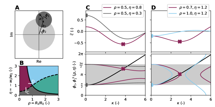
Figure 8: Graphical analysis for extrema of reduced profile for derivation of transition curves. A The condition for the extremum Eq 43 amounts to the addition of two vectors in the complex plane whose sum is purely imaginary. The vectors have lengths $a_{1}$ and $a_{2}$ and angles $\phi_{1}$ and $\phi_{2}$, defined in Eq 44. B Diagram of Fig 3F with indicated parameter combinations $\left(\rho,\eta\right)$ as used in panels C and D. C–D Reduced profile $\widetilde{c}$ (top) and $\phi_{1}$ and $\phi_{1}^{\pm}$ from Eq 45 vs. $\kappa$ (bottom) for two different combinations of $\left(\rho,\eta\right)$ with line colors corresponding to regions in panel B. C $\left|\widetilde{c}_{\mathrm{min}}\right|>\widetilde{c}_{\mathrm{max}}$ in purple and vice versa in dark gray. D $\widetilde{c}_{\mathrm{min}}$ at $\kappa=0$ in light blue and at $\kappa>0$ in purple.

We here use a graphical approach to derive the transition curves shown first in Fig 3F. A necessary condition for an extreme value of the reduced profile $\widetilde{c}\left(\kappa\right)$ from Eq 12 located at $\kappa^{\ast}$ is: $\begin{array}[]{rcl}\frac{\partial}{\partial\kappa}\widetilde{c}\left(\kappa\right)|_{\kappa^{\ast}}&=&0.\end{array}$ With the derivative

$$\frac{\partial}{\partial\kappa}\widetilde{c}\left(\kappa\right)=\frac{\cos\left(\kappa\right)}{\kappa}-\frac{\sin\left(\kappa\right)}{\kappa^{2}}-\eta\frac{\cos\left(\rho\kappa\right)}{\kappa}+\eta\frac{\sin\left(\rho\kappa\right)}{\rho\kappa^{2}},$$ (42)

this condition can be rewritten as

$$\begin{split}0&=\operatorname{Re}\left[\left(\kappa+i\right)\mathrm{e}^{i\kappa}-\frac{\eta}{r}\left(\rho\kappa+i\right)\mathrm{e}^{i\rho\kappa}\right]\\ &=\operatorname{Re}\left[a_{1}\mathrm{e}^{i\phi_{1}}+a_{2}\mathrm{\mathrm{e}}^{i\phi_{2}}\right]\\ &=a_{1}\cos\left(\phi_{1}\right)+a_{2}\cos\left(\phi_{2}\right),\end{split}$$ (43)

where $a_{1}$ and $a_{2}$ are the absolute values of the complex numbers and $\phi_{1}$ and $\phi_{2}$ their phases, given by

$$\begin{split}a_{1}\left(\kappa\right)&=\sqrt{1+\kappa^{2}}\\ \phi_{1}\left(\kappa\right)&=\kappa+\frac{\pi}{2}-\arctan\left(\kappa\right)\\ a_{2}\left(\kappa;\rho,\gamma\right)&=\frac{\eta}{\rho}\sqrt{1+\rho^{2}\kappa^{2}}\\ \phi_{2}\left(\kappa;\rho\right)&=\rho\kappa+\frac{3\pi}{2}-\arctan\left(\rho\kappa\right).\end{split}$$ (44)

The vanishing right-hand-side of Eq 43 implies that the term in the square brackets is purely imaginary. An example solution for the case $a_{1}<a_{2}$ is illustrated in Fig 8A in the complex plane. Note that $a_{1}$ and $\phi_{1}$ are independent of the parameters $\rho$ and $\eta$ in this representation. In our graphical analysis, Eq 43 is interpreted as the sum of two vectors in the complex plane. As shown in Fig 8A, we determine $\phi_{1}$ as the angle at which the tip of the second vector ends on the imaginary axis, which follows from elementary trigonometry as

$$\phi_{1}^{\pm}=\pi\pm\arccos\left(\frac{a_{2}}{a_{1}}\cos\left(\phi_{2}\right)\right).$$ (45)

The locations of extrema are then given by the intersections of $\phi_{1}^{\pm}$ with the second row of Eq 44. Here $\phi_{2}$ is determined from the last equation in Eq 43.

Fig 8B reproduces Fig 3F. The white bars connect points given by parameter combinations $\left(\rho,\eta\right)$ on both sides of the transition curves, and the parameters are specified in panels C and D. The first transition curve $\eta_{t1}\left(\rho\right)$ (dashed line in Fig 8B) is determined by $\widetilde{c}_{\mathrm{max}}\left(\kappa_{\mathrm{max}}\right)=\left|\widetilde{c}_{\mathrm{min}}\left(\kappa_{\mathrm{min}}\right)\right|$, that means it is determined by parameters $\left(\rho,\eta\right)$ for which the absolute values of the positive and negative extremum of the profile are equal. The top panel of Fig 8C compares two reduced profiles obtained for a fixed value for $\rho$ and two values for $\eta$. The line colors correspond to the colored regions in the diagram in Fig 8B for the respective parameter combination $\left|\widetilde{c}_{\mathrm{min}}\right|>\widetilde{c}_{\mathrm{max}}$ for the purple profile and vice versa for the dark gray profile. The point with the maximum absolute value of each profile is indicated with a cross. Exactly at the transition either $\kappa_{\mathrm{max}}$ or $\kappa_{\mathrm{min}}$ is zero (for example $\kappa_{0}=0$) and the other one is non-zero (for example $\kappa_{1}>0$). This condition, with Eq 12, yields the absolute value for both extrema at the transition, where they must be equal, thus $\left|\widetilde{c}\left(\kappa_{0}\right)\right|=\left|\widetilde{c}\left(\kappa_{1}\right)\right|=\left|1-\eta\right|$. Any point on the transition curve is a unique triplet of parameters$\left(\rho,\eta,\kappa_{1}\right)$, and with the condition $\frac{\partial}{\partial\kappa}\widetilde{c}\left(\kappa\right)|_{\kappa_{1}}=0$ we obtain two equations that need to be fulfilled at each point for $\kappa=\kappa_{1}$:

$$\begin{split}1-\eta&=\frac{\sin\left(\kappa\right)}{\kappa}-\eta\frac{\sin\left(\rho\kappa\right)}{\rho\kappa}\\ 1-\eta&=\cos\left(\kappa\right)-\eta\cos\left(\rho\kappa\right).\end{split}$$ (46)

The lower equation is obtained by identifying $\widetilde{c}\left(\kappa\right)$ in its derivative in Eq 42. We solve both equations with respect to $\eta$ and equate them to get

$$\frac{1}{\kappa}\sin\left(\kappa\right)\left[1+\cos\left(\rho\kappa\right)\right]-\frac{1}{\rho\kappa}\sin\left(\rho\kappa\right)\left[1+\cos\left(\kappa\right)\right]+\cos\left(\rho\kappa\right)-\cos\left(\kappa\right)=0.$$ (47)

For a given value of $\rho$, we compute the roots of the left-hand-side expression, which defines $\kappa(\rho)$. The bottom panel of Fig 8C shows $\phi_{1}$ from Eq 44 as a black line and $\phi_{1}^{\pm}$ from Eq 45 for the parameters of the two effective profiles (same color coding as in the top panel). The intersections corresponding to the relevant extrema are highlighted by crosses. This visual analysis allows us to identify the interval for $\kappa$ in which zero-crossings of the left-hand side of Eq 47 as a function of $\kappa$ can correspond to the extrema, that is $\kappa\in\left(0,\,4.49341\right)$ where the lower limit corresponds to $\phi_{1}=\frac{\pi}{2}$ and the upper limit to $\phi_{1}=\frac{3\pi}{2}$. The zero-crossing at the smallest non-zero $\kappa$ indicates the extremum at $\kappa_{1}$. Finally, the transition curve is given by

$$\eta_{t1}\left(\rho\right)=\frac{1+\cos\left(\kappa\left(\rho\right)\right)}{1+\cos\left(\rho\kappa\left(\rho\right)\right)},$$ (48)

where $\kappa(\rho)$ is given by the roots of (47).

The second transition curve $\eta_{t2}\left(\rho\right)$ (solid line in Fig 8B) indicates whether the extremum with the largest absolute value occurs at $\kappa=0$ or at $\kappa>0$. Fig 8D shows in the top panel two reduced profiles for a fixed value of $\eta$, but two values for $\rho$ such that the $\widetilde{c}_{\mathrm{min}}$ occurs once at $\kappa_{\mathrm{min}}=0$ (light blue as in Fig 8B) and once at $\kappa_{\mathrm{min}}>0$ (purple as in Fig 8B), indicated by cross markers.

Graphical analysis using the bottom panel of Fig 8D indicates that this transition happens when $\phi_{1}^{-}$ at $\kappa\gtrsim 0$ switches from lying slightly above (light blue line) to below (purple line) the parameter-independent function $\phi_{1}$ (black line). We observe that decreasing $\rho$ moves the intersection point and with it the location of the extremum up the black line, starting from $\kappa=0$ to larger values for $\kappa$.

Close to the transition, the intersection point comes arbitrarily close to $\kappa=0$, which permits local analysis by a Taylor expansion of $\phi_{1}$ for small $\kappa$:

$$\phi_{1}\left(\kappa\right) \approx\frac{\pi}{2}+\frac{\kappa^{3}}{3}+\mathcal{O}\left(\kappa^{5}\right)$$ (49)

$$\phi_{1}^{-}\left(\kappa;\rho,\eta\right) \approx\frac{\pi}{2}+\frac{\eta\rho\kappa^{3}}{3}+\mathcal{O}\left(\left(\rho\kappa\right)^{5}\right).$$ (50)

A comparison of the coefficients of the third-order polynomials then gives the transition curve

$$\eta_{t2}\left(\rho\right)=\frac{1}{\rho^{2}},$$ (51)

because this coefficient decides for small $\kappa$ whether $\phi_{1}$ (black line) or $\phi_{1}^{-}$ as a function of the parameters $\left(\rho,\eta\right)$ has a larger slope and lies on top.

4.4 Linearization of the spiking model

4.4.1 Fast synaptic noise

The stationary firing rate of a LIF neuron model subject to fast synaptic noise has been derived in [107, 121]. The linear response of the model to time-dependent stimuli has been derived in [104, Eq 29], by application of a general reduction technique to a white noise system with displaced boundary conditions.

Stationary firing rate

The stationary firing rate $\nu_{0}$ in the limit of short synaptic time constants ($\tau_{\mathrm{s}}\ll\tau_{\mathrm{m}}$) is given by [121, 97, Eq A.1]:

$$\begin{split}\nu_{0}^{-1}&=\tau_{\mathrm{r}}+\tau_{\mathrm{m}}\sqrt{\pi}\left(F\left(y_{\theta}\right)-F\left(y_{\mathrm{r}}\right)\right)\\ f\left(y\right)&=\mathrm{e}^{y^{2}}\left(1+\mathrm{erf}\left(y\right)\right),\qquad F\left(y\right)=\int^{y}f\left(y\right)dy\\ \mathrm{\mbox{with}\quad}y_{\left\{\theta,r\right\}}&=\frac{V_{\left\{\theta,r\right\}}-\mu}{\sigma}+\frac{\beta}{2}\sqrt{\frac{\tau_{\mathrm{s}}}{\tau_{\mathrm{m}}}},\qquad\beta=\sqrt{2}\left|\zeta\left(\frac{1}{2}\right)\right|,\end{split}$$ (52)

where $\zeta$ denotes the Riemann’s zeta function [122].

Transfer function

The linear response of the firing rate is described by the transfer function, here denoted by $H_{\mu}$, that relates the modulation of the firing rate $\delta\nu(\omega)$ to the modulation of the mean $\delta\mu(\omega)$ as

$$\delta\nu(\omega) =H_{G}(\omega)\,\delta\mu(\omega)+o(\delta\mu^{2}).$$

It is computed based on the first term of [104, Eq 29]

$$H_{G}\left(\omega\right)=\frac{\nu_{0}\frac{\sqrt{2}}{\sigma}}{1+i\omega\tau_{\mathrm{m}}}\frac{\Phi_{\omega}^{\prime}|_{x\theta}^{x_{\mathrm{r}}}}{\Phi_{\omega}|_{x\theta}^{x_{\mathrm{r}}}},$$ (53)

for the oscillation frequency $\omega$ and the boundaries $x_{\left\{\mathrm{r},\theta\right\}}=\sqrt{2}$$y_{\left\{\theta,r\right\}}$. The function $\Phi_{\omega}\left(x\right)=e^{\frac{1}{4}x^{2}}\,U\left(i\omega\tau_{\mathrm{m}}-\frac{1}{2},x\right)$ is defined by parabolic cylinder functions $U$ [122, 103] and $\Phi_{\omega}^{{}^{\prime}}=\partial_{x}\Phi_{\omega}$. $\Phi_{\omega}|_{x\theta}^{x_{\mathrm{r}}}$ is a short-hand notation for $\Phi_{\omega}\left(x_{\mathrm{r}}\right)-\Phi_{\omega}\left(x_{\theta}\right)$. We need to multiply the transfer function with the transfer function of a first-order low-pass filter due to the exponential time course of our synaptic currents:

$$H_{\mu}\left(\omega\right)=H_{G}\left(\omega\right)\,{\normalcolor}\frac{1}{1+i\omega\tau_{\mathrm{s}}}.$$ (54)

We then obtain $h_{\mu}$ by an inverse Fourier transform and a Laplace transform because $\lambda$ is a complex frequency and $\omega$ is real in the present context:

$$\begin{split}h_{\mu}\left(t\right)&=\mathcal{F}^{-1}\left[H_{\mu}\right]\left(t\right)\\ H_{\mu}\left(\lambda\right)&=\mathcal{L}\left[h_{\mu}\right]\left(\lambda\right).\end{split}$$ (55)

The latter relations imply a replacement $i\omega\to\lambda$ in Eq 53.

For completeness we also provide the term due to the modulation of the variance [104, Eq 29], cf. also Eq 19,

$$H_{\sigma^{2}}(\omega) =\frac{1}{\sigma^{2}}\frac{\nu_{0}}{2+i\omega}\,\frac{\Phi_{\omega}^{\prime\prime}|_{x_{\theta}}^{x_{\mathrm{r}}}}{\Phi_{\omega}|_{x_{\theta}}^{x_{\mathrm{r}}}}.$$

In the fluctuation-driven regime, $H_{\mu}$ and $H_{\sigma^{2}}$ both have a maximum at vanishing frequency. We compare these two contributions in Fig 5B, which shows that $H_{\sigma^{2}}$ can be neglected compared to the former with only making a small error.

4.5 Model comparison

4.5.1 Effective coupling strength

For the numerical evaluation of the transfer function, we show $H_{0}^{\mathrm{ecs}}=w^{\mathrm{ecs}}/\left(\tau_{\mathrm{m}}JK\right)$ as the dashed line in Fig 5B, obtained by calculating analytically the effective coupling strength $w^{\mathrm{ecs}}$ from linear-response theory. The effective coupling strength for a connection from neuron $j$ with rate $\nu_{j}$ to neuron $i$ with rate $\nu_{i}$ is defined as [97, Eqs. A.2 and A.3 (correcting a typo in this previous work)]:

$$\begin{split}w_{ij}^{\mathrm{ecs}}&=\frac{\partial\nu_{i}}{\partial\nu_{j}}\\ &=\widetilde{\alpha}J_{ij}+\widetilde{\beta}J_{ij}^{2}\\ \text{with}\quad\widetilde{\alpha}&=\sqrt{\pi}\left(\tau_{\mathrm{m}}\nu_{i}\right)^{2}\frac{1}{\sigma_{i}}\left(f\left(y_{\theta}\right)-f\left(y_{\mathrm{r}}\right)\right)\\ \text{and}\quad\widetilde{\beta}&=\sqrt{\pi}\left(\tau_{\mathrm{m}}\nu_{i}\right)^{2}\frac{1}{2\sigma_{i}^{2}}\,\left(f\left(y_{\theta}\right)\,y_{\theta}-f\left(y_{\mathrm{r}}\right)\,y_{\mathrm{r}}\right),\end{split}{\normalcolor}$$ (56)

where $f$ and $y_{\left\{\theta,r\right\}}$ are defined as in Eq 52. The dashed line in Fig 5B is given by the term $\propto\widetilde{\alpha}$ alone since we also ignore the small contribution of the variance to the transfer function ($H_{\sigma^{2}}$) of the LIF neuron [104] .

4.5.2 Linear interpolation

To compute the derivative $d\lambda/d\alpha$ given in Eq 31, we use a method for computing the derivative of an implicit function: If $R\left(\alpha,\lambda\right)=0$, it follows that the derivative

$$\frac{\partial\lambda}{\partial\alpha}=-\frac{\partial R/\partial\alpha}{\partial R/\partial\lambda}=:-\frac{R_{\alpha}}{R_{\lambda}}.$$ (57)

With the characteristic equation for the effective transfer function Eq 29, we get

$$R\left(\alpha,\lambda\right)=H_{\alpha}\left(\lambda\right)\cdot\mathrm{e}^{-\lambda d}\cdot\widehat{p}\left(k\right)-1=0.$$ (58)

The partial derivatives of $R$ with respect to $\alpha$ and $\lambda$ are

$$\begin{split}R_{\alpha}&=\mathrm{e}^{-\lambda d}\cdot\widehat{p}\left(k\right)\cdot\frac{\partial H_{\alpha}\left(\lambda\right)}{\partial\alpha}\\ &=\mathrm{e}^{-\lambda d}\cdot\widehat{p}\left(k\right)\cdot\left[H^{\mathrm{s}}\left(\lambda\right)-H^{\mathrm{nf}}\left(\lambda\right)\right],\end{split}$$

and

$$\begin{split}R_{\lambda}&=\widehat{p}\left(k\right)\cdot\frac{\partial}{\partial\lambda}\left[H_{\alpha}\left(\lambda\right)\cdot\mathrm{e}^{-\lambda d}\right]\\ &=\mathrm{e}^{-\lambda d}\cdot\widehat{p}\left(k\right)\cdot\left[\frac{\partial H_{\alpha}\left(\lambda\right)}{\partial\lambda}-d\cdot H_{\alpha}\left(\lambda\right)\right]\\ &=\mathrm{e}^{-\lambda d}\cdot\widehat{p}\left(k\right)\cdot\left[\alpha\frac{\partial H^{\mathrm{s}}\left(\lambda\right)}{\partial\lambda}+\left(1-\alpha\right)\frac{\partial H^{\mathrm{nf}}\left(\lambda\right)}{\partial\lambda}-d\cdot H_{\alpha}\left(\lambda\right)\right]\\ &=\mathrm{e}^{-\lambda d}\cdot\widehat{p}\left(k\right)\cdot\left[\alpha H_{\lambda}^{\mathrm{s}}\left(\lambda\right)+\left(1-\alpha\right)\cdot H_{\lambda}^{\mathrm{nf}}\left(\lambda\right)-d\cdot H_{\alpha}\left(\lambda\right)\right].\end{split}$$ (59)

4.6 Fixing the working point

For the spiking model, we fix the total input to each neuron in terms of its mean $\mu^{*}$ and variance $\sigma^{*}$ to given values. To attain a fixed working point $\left(\mu^{*},\sigma^{*}\right)$, we add to the local contribution from the recurrently connected network (see Eq 15) external excitatory and inhibitory input with Poisson-distributed interspike interval statistics:

$$\begin{split}\mu^{*}&=\mu+\tau_{\mathrm{m}}J\left(\nu_{\mathrm{E,ext}}-g\nu_{\mathrm{I,ext}}\right)\\ \sigma^{*}&=\sigma+\tau_{\mathrm{m}}J^{2}\left(\nu_{\mathrm{E,ext}}+g^{2}\nu_{\mathrm{I,ext}}\right).\end{split}$$ (60)

The excitatory and inhibitory external connection strengths are $J$ and $-gJ$, respectively. The expressions for the excitatory and inhibitory external rates are:

$$\nu_{\mathrm{E,ext}}=\frac{\widetilde{\sigma}^{2}+g\widetilde{\mu}}{1+g}\qquad\text{and$\qquad\nu_{\mathrm{I,ext}}$$\frac{\widetilde{\sigma}^{2}-\widetilde{\mu}}{g\left(1+g\right)}$}$$ (61)

$$\text{with}\qquad\widetilde{\mu}=\frac{\mu^{*}-\mu}{\tau_{\mathrm{m}}J}\qquad\text{and}\qquad\widetilde{\sigma}^{2}=\frac{\left(\sigma^{*}\right)^{2}-\sigma^{2}}{\tau_{\mathrm{m}}J^{2}}.$$

Eq 61 corrects a small inconsistency in a preliminary report of this study [123] which used Eq E.1 in [97] to fix the working point. Accordingly, the values for $\nu_{\mathrm{E,ext}}$ and $\nu_{\mathrm{I,ext}}$ are updated in Table  4, affecting the raster plots in Figs 1 and 7.

4.7 Physical units

The sub-threshold dynamics of the LIF neuron in Eq 13 are, without loss of generality, given in scaled units. In this formulation, $V$, $J$ and $I$ are all quantities with unit Volt. For the parameter-wise comparison with numerical network simulation (for example using NEST [124]), it is useful to consider a description where $I^{{}^{\prime}}$ and $J^{{}^{\prime}}$ represent electric currents in units of Ampere:

$$\begin{split}\tau_{\mathrm{m}}\frac{\mathrm{\partial}V_{i}^{{}^{\prime}}}{\mathrm{\partial}t}&=-\left(V_{i}^{{}^{\prime}}-E_{\mathrm{L}}\right)+R_{\mathrm{m}}I{}_{i}^{{}^{\prime}}\left(t\right)\\ \tau_{\mathrm{s}}\frac{\mathrm{\partial}I_{i}^{{}^{\prime}}}{\mathrm{\partial}t}&=-I_{i}^{{}^{\prime}}+\tau_{\mathrm{s}}\sum_{j}J{}_{ij}^{{}^{\prime}}s_{j}\left(t-d\right).\end{split}$$ (62)

Here, we also introduce a resistive leak reversal potential $E_{\mathrm{L}}$, and shift threshold and reset potentials $V^{\prime}_{\theta}=V_{\theta}+E_{\mathrm{L}}$ and $V^{\prime}_{r}=V_{r}+E_{\mathrm{L}}$, respectively. The membrane time constant $\tau_{\mathrm{m}}=R_{\mathrm{m}}C_{\mathrm{m}}$ relates the membrane resistance $R_{\mathrm{m}}$ and capacitance $C_{\mathrm{m}}$. In units of Ampere, the total current input $I^{{}^{\prime}}=I/R_{\mathrm{m}}$ and the synaptic weight amplitude $J^{{}^{\prime}}=C_{\mathrm{m}}J/\tau_{\mathrm{s}}$.

4.8 Network structure and parameters

Model summary
Populations	Excitatory ($\mathrm{E}$), inhibitory ($\mathrm{I}$)
Topology	Ring network: Neurons positioned equally spaced on one-dimensional domain of length $L$; periodic boundary conditions
Connectivity	Random convergent connections with fixed in-degree, distance-dependent boxcar-shaped spatial profiles realized with cut-off masks
Spiking model
Neuron model	Leaky integrate-and-fire (LIF), fixed threshold, absolute refractory time
Synapse model	Static weights and delays, exponentially shaped postsynaptic currents
Input	Independent fixed-rate Poisson spike trains to all neurons (excitatory and inhibitory Poisson sources)
Measurement	Spike activity
Rate model
Neuron model	Rate neuron with $\mathrm{tanh}$ gain function
Synapse model	Delayed rate connection
Input	-
Measurement	Activity

Table 2: Summary of network models following the guidelines of Nordlie et al. [125]. Separation between nonlinear spiking and rate neurons as used in NEST simulations.

We simulate recurrently connected neural networks of one excitatory and one inhibitory populations each using the neural simulation software NEST [126], using either spiking- or rate-neuron models. The support for rate neurons in NEST was added as described in [108]. Figs 2 and 3 provide the complete neuron and network model descriptions and Table  4 summarizes all parameters as used for the network state showing wave trains (marked by black star in Fig 1D, Fig 4D and Fig 7C). Other simulation parameters used to obtain other network states shown throughout this paper are indicated with a $\varoast$ marker in Table  4, and the changed parameters are given in the corresponding figures. The same marker always denotes the same parameter combination across figure panels. The tables distinguish between network properties and parameters valid for both spiking and rate neuron models and those specific to only one neuron model. Irrespective of the choice of neuron model (rate vs. spiking), the neuron parameters are shared between both neuron populations.

The number of excitatory neurons $N_{\mathrm{E}}$ in our network is four times larger than the number of inhibitory neurons $N_{\mathrm{I}}$ [127]. All neurons are positioned on a grid along a one-dimensional path of perimeter $L$ with a space constant of $\Delta x=L/N_{\mathrm{I}}$. At each grid position $x\in\left[0,L-\Delta x\right]$, there is one inhibitory neuron and four excitatory neurons. The network activity in Figs 1, 4 and 7 is shown for all inhibitory neurons, but only for one excitatory neuron at each grid position. Connections between neurons are drawn according to a distance-dependent rule with periodic boundary conditions (a “ring” network) using the NEST Topology module. The number of incoming connections, the in-degree $K_{\left\{\mathrm{E,I}\right\}}$, is proportional to the population size of the presynaptic population, assuming an overall connection probability of $10\%$. The width of the boxcar-shaped distance-dependent profile $R_{\left\{\mathrm{E,I}\right\}}$ depends on the presynaptic population alone. Within a distance of $R_{\left\{\mathrm{E,I}\right\}}$ around each postsynaptic neuron, potential presynaptic neurons are selected at random and connections are established until the prescribed in-degree is reached. The random component of this connection algorithm may lead to a slight asymmetry with respect to excitation and inhibition in the finite-sized network that might cause a small drift visible for example in stationary Turing patterns as in Fig 4B. Potentially presynaptic neurons within this distance are picked at random and connections are established until the fixed in-degree is reached. Multiple connections between the same pair of neurons termed multapses are allowed, but self-connections (autapses) are prohibited.

The leaky integrate-and-fire model with exponential postsynaptic currents is implemented in NEST under the name iaf_psc_exp. The neuron parameters are the same as in the microcircuit model of [128] with the difference that our membrane time constant $\tau_{\mathrm{m}}$ is half of theirs and that we here omit the refractory period $\tau_{\mathrm{ref}}$, although our results generalize to a non-zero $\tau_{\mathrm{ref}}$. An excitatory and an inhibitory Poisson generator provide external input to all neurons. Their rates $\nu_{\left\{\mathrm{E,I}\right\},\mathrm{ext}}$ are determined according to Eq 61 for fixing the working point $\left(\mu,\sigma\right)$.

The dynamics of rate-based units in NEST is specified as stochastic differential equations using the Itô convention [108], except that we here set the stochasticity (the variance of the input) to zero. We use the neuron model tanh_ipn, that employs a hyperbolic tangent as a gain function.

Simulations run for a simulation time $T_{\mathrm{sim}}$ with a temporal resolution of $dt$. During rate simulations, the instantaneous rate is recorded once at each time step $dt$. Our raster plots from simulations of the spiking model and the image plots from simulation of the rate model show the network activity from all simulated neurons after a start-up transient $T_{\mathrm{trans}}.$

4.9 Software and implementation

Spiking- and rate-neuron network simulations were implemented in NEST v2.18.0 [124], and Python v3.6.9. Post-processing and plotting relied on Python with NumPy v1.16.4, SciPy v1.2.1, and Matplotlib v3.0.2.

Network models
Distance-dependentconnectivity	Neural units $j\in X$ at location $x_{j}$ and $i\in Y$ at $x_{i}$ in pre- and postsynaptic populations $X$ and $Y$, respectively. Displacement between units $i$ and $j$: $r_{ij}=x_{i}-x_{j}$ Boxcar-shaped spatial profile with width $R$ and Heaviside function $\Theta$: $p\left(r_{ij}\right)=\frac{1}{2R}\Theta\left(R-\left|r_{ij}\right|\right)$
Spiking model
Subthresholddynamics	If $t>t^{*}+\tau_{\mathrm{ref}}$ $\frac{\mathrm{\partial}V}{\partial t}=-\frac{V-E_{\mathrm{L}}}{\tau_{\mathrm{m}}}+\frac{I_{\mathrm{syn}}\left(t\right)}{C_{\mathrm{m}}}$ $I_{\mathrm{syn}}\left(t\right)=\sum_{j}J_{j}I_{\mathrm{PSC}}\left(t-t_{j}^{*}-d\right)$ with connection strength $J_{j}$, presynaptic spike time $t_{j}^{*}$ and conduction delay $d$ $I_{\mathrm{PSC}}\left(t\right)=\mathrm{e}^{-t/\tau_{\mathrm{s}}}\Theta\left(t\right)$ with Heaviside function $\Theta$ else $V\left(t\right)=V_{r}$
Spiking	If $V\left(t-\right)<V_{\theta}\wedge V\left(t+\right)\geq V_{\theta}$ 1. set $t^{*}=t$ 2. emit spike with timestamp $t^{*}$ 3. reset $V\left(t\right)=V_{\mathrm{r}}$
Rate model
Differentialequation	$\tau\frac{\mathrm{\partial}u}{\mathrm{\partial}t}\left(t\right)=-u\left(t\right)+\sum_{j=1}w_{j}\psi\left(u_{j}\left(t-d\right)\right)$ with the nonlinearity $\psi\left(u\right)=\tanh\left(u\right)$

Table 3: Description of network models. Separation between nonlinear spiking and rate neurons as used in NEST simulations.

A: Global simulation parameters
Symbol	Value	Description
$T_{\mathrm{sim}}$	$350\,\mathrm{ms}$	Simulation duration
$T_{\mathrm{trans}}$	$150\,\mathrm{ms}$	Start-up transient
$dt$	$0.1\,\mathrm{ms}$	Temporal resolution

B: Populations and external input
Symbol	Value	Description
$N_{\mathrm{E}}$	$4,000$	Population size of excitatory neurons
$N_{\mathrm{I}}$	$1,000$	Population size of inhibitory neurons
$L$	$1\,\mathrm{mm}$	Domain length
Spiking model
$\mu^{*}$	$10\,\mathrm{mV}$	Mean input relative to resting potential
$\sigma^{*}$	$10\,\mathrm{mV}$	Variance of input relative to resting potential
$\nu_{\mathrm{E,ext}}$	$96,463\,\mathrm{Hz}$	$\varoast$ Excitatory external rate (by fixing working point)
$\nu_{\mathrm{I,ext}}$	$15,958\,\mathrm{Hz}$	$\varoast$ Inhibitory external rate (by fixing working point)

C: Connection parameters
Symbol	Value	Description
$R_{\mathrm{E}}$	$0.2\,\mathrm{mm}$	$\varoast$ Profile width of excitatory neurons
$R_{\mathrm{I}}$	$0.07\,\mathrm{mm}$	$\varoast$ Profile width of inhibitory neurons
$d$	$3\,\mathrm{ms}$	$\varoast$ Delay
Spiking model
$K_{\mathrm{E}}$	$400$	In-degree from excitatory neurons
$\gamma$	$0.25$	Relative in-degree, $\gamma=K_{\mathrm{I}}/K_{\mathrm{E}}$
$J_{\mathrm{E}}^{{}^{\prime}}$	$87.8\,\mathrm{pA}$	$\varoast$ Reference synaptic strength
$g$	$5$	$\varoast$ Relative synaptic strength, $g=-J_{\mathrm{I}}/J_{\mathrm{E}}$
Rate model
$w_{\mathrm{E}}$	$2.73$	$\varoast$ Excitatory weight (by parameter mapping)
$w_{\mathrm{I}}$	$-3.42$	$\varoast$ Inhibitory weight (by parameter mapping)

D: Neuron model
Symbol	Value	Description
Spiking model
$C_{\mathrm{m}}$	$250\,\mathrm{pF}$	Membrane capacitance
$\tau_{\mathrm{m}}$	$5\,\mathrm{ms}$	Membrane time constant
$E_{\mathrm{L}}$	$-65\,\mathrm{mV}$	Resting potential
$V_{\theta}$	$-50\,\mathrm{mV}$	Firing threshold
$V_{\mathrm{r}}$	$-65\,\mathrm{mV}$	Reset potential
$\tau_{\mathrm{ref}}$	$0\,\mathrm{ms}$	Absolute refractory period
$\tau_{\mathrm{\mathrm{s}}}$	$0.5\,\mathrm{ms}$	Postsynaptic current time constant
Rate model
$\tau$	$1.94\,\mathrm{ms}$	Time constant (by parameter mapping)

Table 4: Simulation and network parameters. Parameters according to setting for wave trains as shown in Fig 1D, Fig 4D and Fig 7C (black star marker). Deviant parameters are given in the captions of the respective figures and indicated by different markers.

Funding

This project has received funding from the Helmholtz association: portfolio Supercomputing and Modeling for the Human Brain (SMHB), young investigator group VH-NG-1028; the European Union’s Horizon 2020 research and innovation programme under grant agreement No 720270 (HBP SGA1), the German Research Foundation (DFG; grant DI 1721/3-1 [KFO219-TP9]), the ERS grant "Facing the multi-scale problem in neuroscience" of the RWTH Aachen University, and the Research Council of Norway (NFR) through COBRA (grant No 250128). The funders had no role in study design, data collection and analysis, decision to publish, or preparation of the manuscript.

References

- 1. Rubino D, Robbins KA, Hatsopoulos NG. Propagating waves mediate information transfer in the motor cortex. 2006;9(12):1549–1557. doi:10.1038/nn1802.
- 2. Nauhaus I, Busse L, Carandini M, Ringach DL. Stimulus contrast modulates functional connectivity in visual cortex. 2009;12:70–76. doi:10.1038/nn.2232.
- 3. Muller L, Destexhe A. Propagating waves in thalamus, cortex and the thalamocortical system: Experiments and models. 2012;106(5-6):222–238. doi:10.1016/j.jphysparis.2012.06.005.
- 4. Sato TK, Nauhaus I, Carandini M. Traveling Waves in Visual Cortex. 2012;75(2):218–229. doi:10.1016/j.neuron.2012.06.029.
- 5. Muller L, Reynaud A, Chavane F, Destexhe A. The stimulus-evoked population response in visual cortex of awake monkey is a propagating wave. Nature Communications. 2014;5. doi:10.1038/ncomms4675.
- 6. Townsend RG, Solomon SS, Chen SC, Pietersen ANJ, Martin PR, Solomon SG, et al. Emergence of Complex Wave Patterns in Primate Cerebral Cortex. 2015;35(11):4657–4662. doi:10.1523/jneurosci.4509-14.2015.
- 7. Zanos TP, Mineault PJ, Nasiotis KT, Guitton D, Pack CC. A Sensorimotor Role for Traveling Waves in Primate Visual Cortex. 2015;85(3):615–627. doi:10.1016/j.neuron.2014.12.043.
- 8. Denker M, Zehl L, Kilavik BE, Diesmann M, Brochier T, Riehle A, et al. LFP beta amplitude is linked to mesoscopic spatio-temporal phase patterns. Scientific Reports. 2018;8(1):1–21. doi:10.1038/s41598-018-22990-7.
- 9. Kim U, Bal T, McCormick DA. Spindle waves are propagating synchronized oscillations in the ferret LGNd in vitro. 1995;74(3):1301–1323. doi:10.1152/jn.1995.74.3.1301.
- 10. Lubenov EV, Siapas AG. Hippocampal theta oscillations are travelling waves. 2009;459(7246):534–539. doi:10.1038/nature08010.
- 11. Riehle A, Wirtssohn S, Grün S, Brochier T. Mapping the spatio-temporal structure of motor cortical LFP and spiking activities during reach-to-grasp movements. Frontiers in Neural Circuits. 2013;7:48. doi:10.3389/fncir.2013.00048.
- 12. Takahashi K, Kim S, Coleman TP, Brown KA, Suminski AJ, Best MD, et al. Large-scale spatiotemporal spike patterning consistent with wave propagation in motor cortex. Nature Communications. 2015;6(7169). doi:10.1038/ncomms8169.
- 13. Ferezou I, Bolea S, Petersen CCH. Visualizing the Cortical Representation of Whisker Touch: Voltage-Sensitive Dye Imaging in Freely Moving Mice. 2006;50(4):617–629. doi:10.1016/j.neuron.2006.03.043.
- 14. Garaschuk O, Linn J, Eilers J, Konnerth A. Large-scale oscillatory calcium waves in the immature cortex. 2000;3(5):452–459. doi:10.1038/74823.
- 15. Mehring C, Hehl U, Kubo M, Diesmann M, Aertsen A. Activity dynamics and propagation of synchronous spiking in locally connected random networks. 2003;88(5):395–408. doi:10.1007/s00422-002-0384-4.
- 16. Yger P, El Boustani S, Destexhe A, Frégnac Y. Topologically invariant macroscopic statistics in balanced networks of conductance-based integrate-and-fire neurons. 2011;31:229–245. doi:10.1007/s10827-010-0310-z.
- 17. Voges N, Perrinet L. Complex dynamics in recurrent cortical networks based on spatially realistic connectivities. 2012;6:41. doi:10.3389/fncom.2012.00041.
- 18. Keane A, Gong P. Propagating Waves Can Explain Irregular Neural Dynamics. 2015;35(4):1591–1605. doi:10.1523/jneurosci.1669-14.2015.
- 19. Voges N, Schüz A, Aertsen A, Rotter S. A modeler’s view on the spatial structure of intrinsic horizontal connectivity in the neocortex. 2010;92(3):277–292. doi:10.1016/j.pneurobio.2010.05.001.
- 20. Hellwig B. A quantitative analysis of the local connectivity between pyramidal neurons in layers 2/3 of the rat visual cortex. 2000;2(82):111–121. doi:10.1007/pl00007964.
- 21. Perin R, Berger TK, Markram H. A synaptic organizing principle for cortical neuronal groups. 2011;108(13):5419–5424. doi:10.1073/pnas.1016051108.
- 22. Schnepel P, Kumar A, Zohar M, Aertsen A, Boucsein C. Physiology and Impact of Horizontal Connections in Rat Neocortex. 2015;25(10):3818–3835. doi:10.1093/cercor/bhu265.
- 23. Wilson HR, Cowan JD. Excitatory and Inhibitory Interactions in Localized Populations of Model Neurons. Biophysical Journal. 1972;12(1):1 – 24. doi:http://dx.doi.org/10.1016/S0006-3495(72)86068-5.
- 24. Wilson HR, Cowan JD. A mathematical theory of the functional dynamics of cortical and thalamic nervous tissue. Kybernetik. 1973;13(2):55–80. doi:10.1007/BF00288786.
- 25. Amari SI. Dynamics of Pattern Formation in Lateral-Inhibition Type Neural Fields. 1977;27(2):77–87. doi:10.1007/bf00337259.
- 26. Erlhagen W. Lokalisierte, stationäre Verteilung in neuronalen Feldern: Modellierung experimenteller Befunde zur Planung und Kontrolle zielgerichteter Bewegungen. Thun, Frankfurt/Main: Verlag Harri Deutsch; 1997.
- 27. Bressloff PC, Carroll SR. Laminar Neural Field Model of Laterally Propagating Waves of Orientation Selectivity. 2015;11(10):e1004545. doi:10.1371/journal.pcbi.1004545.
- 28. Ermentrout B. Neural networks as spatio-temporal pattern-forming systems. Reports on Progress in Physics. 1998;61(4):353–430. doi:10.1088/0034-4885/61/4/002.
- 29. Coombes S. Waves, bumps, and patterns in neural field theories. 2005;93:91–108. doi:10.1007/s00422-005-0574-y.
- 30. Wyller J, Blomquist P, Einevoll GT. On the origin and properties of two-population neural field models - a tutorial introduction. Biophysical Reviews and Letters. 2007;02(01):79–98. doi:10.1142/s1793048007000441.
- 31. Coombes S. Large-scale neural dynamics: Simple and complex. NeuroImage. 2010;52(3):731–739. doi:10.1016/j.neuroimage.2010.01.045.
- 32. Bressloff PC. Spatiotemporal dynamics of continuum neural fields. Journal of Physics A: Mathematical and Theoretical. 2012;45(3):033001. doi:10.1088/1751-8113/45/3/033001.
- 33. Bressloff PC. Waves in Neural Media. Springer New York; 2014. Available from: https://doi.org/10.1007/978-1-4614-8866-8.
- 34. Coombes S, bei Graben P, Potthast R, Wright J. Neural Fields. Theory and Applications. Springer-Verlag Berlin Heidelberg; 2014.
- 35. Ermentrout GB, Cowan JD. Temporal oscillations in neuronal nets. 1979;7(3):265–280. doi:10.1007/bf00275728.
- 36. Ermentrout GB, Cowan JD. A mathematical theory of visual hallucination patterns. 1979;34(3):137–150. doi:10.1007/bf00336965.
- 37. Ermentrout BG, Cowan JD. Large Scale Spatially Organized Activity in Neural Nets. 1980;38(1):1–21. doi:10.1137/0138001.
- 38. Ermentrout GB, Cowan JD. Secondary Bifurcation in Neuronal Nets. SIAM Journal on Applied Mathematics. 1980;39(2):323–340. doi:10.1137/0139028.
- 39. Bressloff PC. New Mechanism for Neural Pattern Formation. 1996;76(24):4644–4647. doi:10.1103/physrevlett.76.4644.
- 40. Hutt A, Bestehorn M, Wennekers T. Pattern formation in intracortical neuronal fields. Network: Computation in Neural Systems. 2003;14(2):351–368. doi:10.1088/0954-898x_14_2_310.
- 41. Bressloff PC, Kilpatrick ZP. Nonlocal Ginzburg-Landau equation for cortical pattern formation. 2008;78(4). doi:10.1103/physreve.78.041916.
- 42. Roxin A, Brunel N, Hansel D. The role of delays in shaping spatio-temporal dynamics of neuronal activity in large networks. 2005;94(23):238103. doi:10.1103/physrevlett.94.238103.
- 43. Atay FM, Hutt A. Neural Fields with Distributed Transmission Speeds and Long-Range Feedback Delays. SIAM Journal on Applied Dynamical Systems. 2006;5(4):670–698. doi:10.1137/050629367.
- 44. Venkov NA, Coombes S, Matthews PC. Dynamic instabilities in scalar neural field equations with space-dependent delays. Physica D: Nonlinear Phenomena. 2007;232(1):1–15. doi:10.1016/j.physd.2007.04.011.
- 45. Coombes S, Venkov NA, Shiau L, Bojak I, Liley DTJ, Laing CR. Modeling electrocortical activity through improved local approximations of integral neural field equations. 2007;76(5). doi:10.1103/physreve.76.051901.
- 46. Turing AM. The Chemical Basis of Morphogenesis. Phil Transact Royal Soc. 1952;237:37–72. doi:10.1098/rstb.1952.0012.
- 47. Kuramoto Y. Chemical Oscillations, Waves, and Turbulence. Springer Berlin Heidelberg; 1984. Available from: https://doi.org/10.1007/978-3-642-69689-3.
- 48. Hutt A, Atay FM. Analysis of nonlocal neural fields for both general and gamma-distributed connectivities. Physica D: Nonlinear Phenomena. 2005;203(1-2):30–54. doi:10.1016/j.physd.2005.03.002.
- 49. Wyller J, Blomquist P, Einevoll GT. Turing instability and pattern formation in a two-population neuronal network model. Physica D: Nonlinear Phenomena. 2007;225(1):75–93. doi:10.1016/j.physd.2006.10.004.
- 50. Folias SE, Ermentrout GB. Bifurcations of Stationary Solutions in an Interacting Pair of E-I Neural Fields. SIAM Journal on Applied Dynamical Systems. 2012;11(3):895–938. doi:10.1137/110860094.
- 51. Roxin A, Brunel N, Hansel D. Rate Models with Delays and the Dynamics of Large Networks of Spiking Neurons. Progress of Theoretical Physics Supplement. 2006;161:68–85. doi:10.1143/ptps.161.68.
- 52. Jirsa VK, Kelso JAS. Spatiotemporal pattern formation in neural systems with heterogeneous connection topologies. 2000;62(6):8462–8465. doi:10.1103/physreve.62.8462.
- 53. Atay FM, Hutt A. Stability and bifurcations in neural fields with finite propagation speed and general connectivity. SIAM Journal on Applied Mathematics. 2005;65(2):664–666. doi:10.1137/S0036139903430884.
- 54. Hutt A. Local excitation-lateral inhibition interaction yields oscillatory instabilities in nonlocally interacting systems involving finite propagation delay. 2008;372(5):541–546. doi:10.1016/j.physleta.2007.08.018.
- 55. Bojak I, Liley DTJ. Axonal Velocity Distributions in Neural Field Equations. 2010;6(1):e1000653. doi:10.1371/journal.pcbi.1000653.
- 56. Hutt A, Rougier N. Activity spread and breathers induced by finite transmission speeds in two-dimensional neural fields. 2010;82(5). doi:10.1103/physreve.82.055701.
- 57. Veltz R. An analytical method for computing Hopf bifurcation curves in neural field networks with space-dependent delays. Comptes Rendus Mathematique. 2011;349(13-14):749–752. doi:10.1016/j.crma.2011.06.014.
- 58. Veltz R. Interplay Between Synaptic Delays and Propagation Delays in Neural Field Equations. SIAM Journal on Applied Dynamical Systems. 2013;12(3):1566–1612. doi:10.1137/120889253.
- 59. Faye G, Faugeras O. Some theoretical and numerical results for delayed neural field equations. Physica D: Nonlinear Phenomena. 2010;239(9):561–578. doi:10.1016/j.physd.2010.01.010.
- 60. Veltz R, Faugeras O. Stability of the stationary solutions of neural field equations with propagation delays. The Journal of Mathematical Neuroscience. 2011;1(1):1. doi:10.1186/2190-8567-1-1.
- 61. Dijkstra K, Gils S, Janssens S, Kuznetsov Y, Visser S. Pitchfork–Hopf bifurcations in 1D neural field models with transmission delays. Physica D: Nonlinear Phenomena. 2015;297. doi:10.1016/j.physd.2015.01.004.
- 62. Visser S, Nicks R, Faugeras O, Coombes S. Standing and travelling waves in a spherical brain model: The Nunez model revisited. Physica D: Nonlinear Phenomena. 2017;349:27 – 45. doi:https://doi.org/10.1016/j.physd.2017.02.017.
- 63. Softky WR, Koch C. The Highly Irregular Firing of Cortical Cells Is Inconsistent with Temporal Integration of Random EPSPs. 1993;13(1):334–350. doi:10.1523/jneurosci.13-01-00334.1993.
- 64. Brunel N, Hakim V. Fast Global Oscillations in Networks of Integrate-and-Fire Neurons with Low Firing Rates. 1999;11(7):1621–1671. doi:10.1162/089976699300016179.
- 65. Ecker AS, Berens P, Keliris GA, Bethge M, Logothetis NK. Decorrelated Neuronal Firing in Cortical Microcircuits. 2010;327(5965):584–587. doi:10.1126/science.1179867.
- 66. Hutt A, Hashemi M, beim Graben P. How to Render Neural Fields More Realistic. In: Validating Neuro-Computational Models of Neurological and Psychiatric Disorders. Springer International Publishing; 2015. p. 141–159. Available from: https://doi.org/10.1007/978-3-319-20037-8_6.
- 67. Montbrió E, Pazó D, Roxin A. Macroscopic Description for Networks of Spiking Neurons. Phys Rev X. 2015;5:021028. doi:10.1103/PhysRevX.5.021028.
- 68. Amit DJ, Brunel N. Dynamics of a recurrent network of spiking neurons before and following learning. 1997;8(4):373–404. doi:10.1088/0954-898x_8_4_003.
- 69. Brunel N. Dynamics of sparsely connected networks of excitatory and inhibitory spiking neurons. 2000;8(3):183–208. doi:10.1023/a:1008925309027.
- 70. Lindner B, Doiron B, Longtin A. Theory of oscillatory firing induced by spatially correlated noise and delayed inhibitory feedback. 2005;72(6):061919. doi:10.1103/physreve.72.061919.
- 71. Delarue F, Inglis J, Rubenthaler S, Tanré E. Global solvability of a networked integrate-and-fire model of McKean–Vlasov type. Ann Appl Probab. 2015;25(4):2096–2133. doi:10.1214/14-AAP1044.
- 72. Esnaola-Acebes JM, Roxin A, Avitabile D, Montbrió E. Synchrony-induced modes of oscillation of a neural field model. Phys Rev E. 2017;96:052407. doi:10.1103/PhysRevE.96.052407.
- 73. Golomb D, Ermentrout GB. Bistability in Pulse Propagation in Networks of Excitatory and Inhibitory Populations. 2001;86(18):4179–4182. doi:10.1103/physrevlett.86.4179.
- 74. Cremers D, Herz AVM. Traveling Waves of Excitation in Neural Field Models: Equivalence of Rate Descriptions and Integrate-and-Fire Dynamics. 2002;14(7):1651–1667. doi:10.1162/08997660260028656.
- 75. Osan R, Ermentrout GB. The evolution of synaptically generated waves in one- and two-dimensional domains. 2002;163:217–235. doi:10.1016/s0167-2789(02)00347-0.
- 76. Fohlmeister C, Gerstner W, Ritz R, van Hemmen JL. Spontaneous Excitations in the Visual Cortex: Stripes, Spirals, Rings, and Collective Bursts. 1995;7(5):905–914. doi:10.1162/neco.1995.7.5.905.
- 77. Kistler WM, Seitz R, van Hemmen JL. Modeling collective excitations in cortical tissue. Physica D: Nonlinear Phenomena. 1998;114(3-4):273–295. doi:10.1016/s0167-2789(97)00195-4.
- 78. Kistler WM. Stability properties of solitary waves and periodic wave trains in a two-dimensional network of spiking neurons. 2000;62(6):8834–8837. doi:10.1103/physreve.62.8834.
- 79. Bressloff PC. Traveling waves and pulses in a one-dimensional network of excitable integrate-and-fire neurons. 2000;40(2):169–198. doi:10.1007/s002850050008.
- 80. Crook SM, Ermentrout GB, Vanier MC, Bower JM. The Role of Axonal Delay in the Synchronization of Networks of Coupled Cortical Oscillators. 1997;4(2):161–172. doi:10.1023/a:1008843412952.
- 81. Ermentrout B. Reduction of Conductance-Based Models with Slow Synapses to Neural Nets. 1994;6(4):679–695. doi:10.1162/neco.1994.6.4.679.
- 82. Bressloff PC, Coombes S. Spike Train Dynamics Underlying Pattern Formation in Integrate-and-Fire Oscillator Networks. 1998;81(11):2384–2387. doi:10.1103/physrevlett.81.2384.
- 83. Bressloff PC, Coombes S. A Dynamical Theory of Spike Train Transitions in Networks of Integrate-and-Fire Oscillators. SIAM Journal on Applied Mathematics. 2000;60(3):820–841. doi:10.1137/s0036139998339643.
- 84. Haken H. Quasi-discreted dynamics of a neural net: The lighthouse model. Discrete Dynamics in Nature and Society. 2000;4(3):187–200. doi:10.1155/s1026022600000182.
- 85. Haken H. Phase Locking in the Lighthouse Model of a Neural Net with Several Delay Times. Progress of Theoretical Physics Supplement. 2000;139:96–111. doi:10.1143/ptps.139.96.
- 86. Chow CC, Coombes S. Existence and Wandering of Bumps in a Spiking Neural Network Model. SIAM Journal on Applied Dynamical Systems. 2006;5(4):552–574. doi:10.1137/060654347.
- 87. Laing CR, Chow CC. Stationary Bumps in Networks of Spiking Neurons. 2001;13:1473–1494. doi:10.1162/089976601750264974.
- 88. Rosenbaum R, Doiron B. Balanced Networks of Spiking Neurons with Spatially Dependent Recurrent Connections. Physical Review X. 2014;4(2):021039. doi:10.1103/PhysRevX.4.021039.
- 89. Rosenbaum R, Smith MA, Kohn A, Rubin JE, Doiron B. The spatial structure of correlated neuronal variability. 2017;20(1):107–114. doi:10.1038/nn.4433.
- 90. Pyle R, Rosenbaum R. Spatiotemporal Dynamics and Reliable Computations in Recurrent Spiking Neural Networks. 2017;118(1). doi:10.1103/physrevlett.118.018103.
- 91. Spreizer S, Aertsen A, Kumar A. From space to time: Spatial inhomogeneities lead to the emergence of spatio-temporal activity sequences in spiking neuronal networks. 2018;doi:10.1101/428649.
- 92. Kriener B, Helias M, Rotter S, Diesmann M, Einevoll GT. How pattern formation in ring networks of excitatory and inhibitory spiking neurons depends on the input current regime. 2014;7(187):187. doi:10.3389/fncom.2013.00187.
- 93. Avitable D, Wedgwood KCA. Macroscopic coherent structures in a stochastic neural network: from interface dynamics to coarse-grained bifurcation analysis. Journal of Mathematical Biology. 2017;75(4):885–928. doi:10.1007/s00285-016-1070-9.
- 94. Senk J, Korvasová K, Schuecker J, Hagen E, Tetzlaff T, Diesmann M, et al. Conditions for traveling waves in spiking neural networks obtained from a rigorous mapping to a neural-field model. In: 26th Annual Computational Neuroscience Meeting (CNS*2017), BMC Neuroscience 2017, 18(Suppl 1):P94; 2017.Available from: https://doi.org/10.1186/s12868-017-0371-2.
- 95. Corless RM, Gonnet GH, Hare DEG, Jeffrey DJ, Knuth DE. On the Lambert W function. Advances in Computational Mathematics. 1996;5(1):329–359. doi:10.1007/BF02124750.
- 96. van Vreeswijk C, Sompolinsky H. Chaos in Neuronal Networks with Balanced Excitatory and Inhibitory Activity. 1996;274:1724–1726. doi:10.1126/science.274.5293.1724.
- 97. Helias M, Tetzlaff T, Diesmann M. Echoes in correlated neural systems. 2013;15:023002. doi:10.1088/1367-2630/15/2/023002.
- 98. Fourcaud-Trocmé N, Brunel N. Dynamics of the Instantaneous Firing Rate in Response to Changes in Input Statistics. 2005;18(3):311–321. doi:10.1007/s10827-005-0337-8.
- 99. Ricciardi LM, Di Crescenzo A, Giorno V, Nobile AG. An Outline of Theoretical and Algorithmic Approaches to First Passage Time Problems with Applications to Biological Modeling. 1999;50(2):247–322.
- 100. Risken H. The Fokker-Planck Equation. Springer Verlag Berlin Heidelberg; 1996. Available from: https://doi.org/10.1007/978-3-642-61544-3_4.
- 101. Tuckwell HC. Introduction to Theoretical Neurobiology. vol. 2. Cambridge: Cambridge University Press; 1988.
- 102. Richardson MJE. Firing-rate response of linear and nonlinear integrate-and-fire neurons to modulated current-based and conductance-based synaptic drive. 2007;76(021919):1–15.
- 103. Lindner B, Schimansky-Geier L. Transmission of noise coded versus additive signals through a neuronal ensemble. 2001;86:2934–2937. doi:10.1103/physrevlett.86.2934.
- 104. Schuecker J, Diesmann M, Helias M. Modulated escape from a metastable state driven by colored noise. 2015;92:052119. doi:10.1103/PhysRevE.92.052119.
- 105. Moreno-Bote R, Parga N. Auto- and crosscorrelograms for the spike response of leaky integrate-and-fire neurons with slow synapses. 2006;96:028101.
- 106. Moreno-Bote R, Parga N. Response of Integrate-and-Fire Neurons to Noisy Inputs Filtered by Synapses with Arbitrary Timescales: Firing Rate and Correlations. 2010;22(6):1528–1572. doi:10.1162/neco.2010.06-09-1036.
- 107. Brunel N, Chance FS, Fourcaud N, Abbott LF. Effects of Synaptic Noise and Filtering on the Frequency Response of Spiking Neurons. 2001;86(10):2186–2189. doi:10.1103/physrevlett.86.2186.
- 108. Hahne J, Dahmen D, Schuecker J, Frommer A, Bolten M, Helias M, et al. Integration of continuous-time dynamics in a spiking neural network simulator. 2017;11:34. doi:10.3389/fninf.2017.00034.
- 109. Peyser A, Sinha A, Vennemo SB, Ippen T, Jordan J, Graber S, et al.. NEST 2.14.0; 2017. Available from: https://doi.org/10.10.5281/zenodo.882970.
- 110. Eccles JC, P F, Koketsu K. Cholinergic and inhibitory synapses in a pathway from motor-axon collaterals to motoneurones. 1954;126(3):524–562. doi:10.1113/jphysiol.1954.sp005226.
- 111. Stepanyants A, Martinez LM, Ferecskó AS, Kisvárday ZF. The fractions of short- and long-range connections in the visual cortex. 2009;106(9):3555–3560. doi:10.1073/pnas.0810390106.
- 112. Cross MC, Hohenberg PC. Pattern formation outside of equilibrium. Reviews of Modern Physics. 1993;65(3):851–1112. doi:10.1103/revmodphys.65.851.
- 113. Legenstein R, Maass W. Edge of chaos and prediction of computational performance for neural circuit models. 2007;20(3):323–334. doi:10.1016/j.neunet.2007.04.017.
- 114. Girard P, Hupé JM, Bullier J. Feedforward and Feedback Connections Between Areas V1 and V2 of the Monkey Have Similar Rapid Conduction Velocities. 2001;85(3):1328–1331.
- 115. Muller L, Chavane F, Reynolds J, Sejnowski TJ. Cortical travelling waves: mechanisms and computational principles. 2018;19(5):255–268. doi:10.1038/nrn.2018.20.
- 116. Fermani F, Richardson MJE. Coarse-grained description of the spatio-temporal dynamics of network activity from experimentally verified single-neuron models and connectivity. In: 24th Annual Computational Neuroscience Meeting: CNS*2015, BMC Neuroscience 2015, 16(Suppl 1):P206; 2015.Available from: https://doi.org/10.1186/1471-2202-16-s1-p206.
- 117. Nordlie E, Tetzlaff T, Einevoll GT. Rate dynamics of leaky integrate-and-fire neurons with strong synapses. 2010;4:149. doi:10.3389/fncom.2010.00149.
- 118. Heiberg T, Kriener B, Tetzlaff T, Casti A, Einevoll GT, Plesser HE. Firing-rate models capture essential response dynamics of LGN relay cells. 2013;35(3):359–375. doi:10.1007/s10827-013-0456-6.
- 119. Casti A, Hayot F, Xiao Y, Kaplan E. A simple model of retina-LGN transmission. 2008;24(2):235–252. doi:10.1007/s10827-007-0053-7.
- 120. Gerstner W. Population dynamics of spiking neurons: fast transients, asynchronous states, and locking. 2000;12(1):43–89. doi:10.1162/089976600300015899.
- 121. Fourcaud N, Brunel N. Dynamics of the firing probability of noisy integrate-and-fire neurons. 2002;14(9):2057–2110. doi:10.1162/089976602320264015.
- 122. Abramowitz M, Stegun IA. Handbook of Mathematical Functions: with Formulas, Graphs, and Mathematical Tables. New York: Dover Publications; 1974. Available from: https://doi.org/10.1119/1.15378.
- 123. Senk J, Korvasová K, Schuecker J, Hagen E, Tetzlaff T, Diesmann M, et al. Conditions for traveling waves in spiking neural networks. arXiv preprint arXiv:180106046v1. 2018;.
- 124. Jordan J, Mørk H, Vennemo SB, Terhorst D, Peyser A, Ippen T, et al.. NEST 2.18.0; 2019. Available from: http://doi.org/10.5281/zenodo.2605422.
- 125. Nordlie E, Tetzlaff T, Einevoll GT. Firing-rate response properties of spiking neurons: beyond the diffusion limit. 2009;.
- 126. Gewaltig MO, Diesmann M. NEST (NEural Simulation Tool). Scholarpedia. 2007;2(4):1430. doi:10.4249/scholarpedia.1430.
- 127. Braitenberg V. Brain size and number of neurons: an exercise in synthetic neuroanatomy. 2001;10(1):71–77. doi:10.1023/a:1008920127052.
- 128. Potjans TC, Diesmann M. The Cell-Type Specific Cortical Microcircuit: Relating Structure and Activity in a Full-Scale Spiking Network Model. 2014;24(3):785–806. doi:10.1093/cercor/bhs358.