Spin networks on adiabatic quantum computer

Abstract

The article is addressing a possibility of implementation of spin network states on adiabatic quantum computer. The discussion is focused on application of currently available technologies and analyzes a concrete example of D-Wave machine. A class of simple spin network states which can be implemented on the Chimera graph architecture of the D-Wave quantum processor is introduced. However, extension beyond the currently available quantum processor topologies is required to simulate more sophisticated spin network states, which may inspire development of new generations of adiabatic quantum computers. A possibility of simulating Loop Quantum Gravity is discussed and a method of solving a graph non-changing scalar (Hamiltonian) constraint with the use of adiabatic quantum computations is proposed.

1 Introduction

One can distinguish two main modes of operation of quantum computers. The first is quantum data processing associated mostly with implementation on quantum algorithms with the use of quantum gates or various quantum machine learning protocols [1]. The second concerns simulations of quantum systems.

Simulating quantum system with the use quantum computers is fundamentally different from what simulations performed at classical computers are. While classical simulations rely on either discretization of a given physical system or an adequate algebraic analysis the simulations performed on quantum computers allow to imitate a given quantum systems. This kind of exact simulation of a quantum system has been a subject of discussion in a seminal R. Feynman article [2].

In order to understand better what we mean by exact simulations let us consider the case of Planck scale physics. Here, the relevant degrees of freedom are defined at length scales of the order of the Planck length $l_{\rm Pl}\sim 10^{-35}$m. Despite significant advances made in both theoretical understanding and experimental techniques, the Planck scale physics remains empirically inaccessible for the moment.

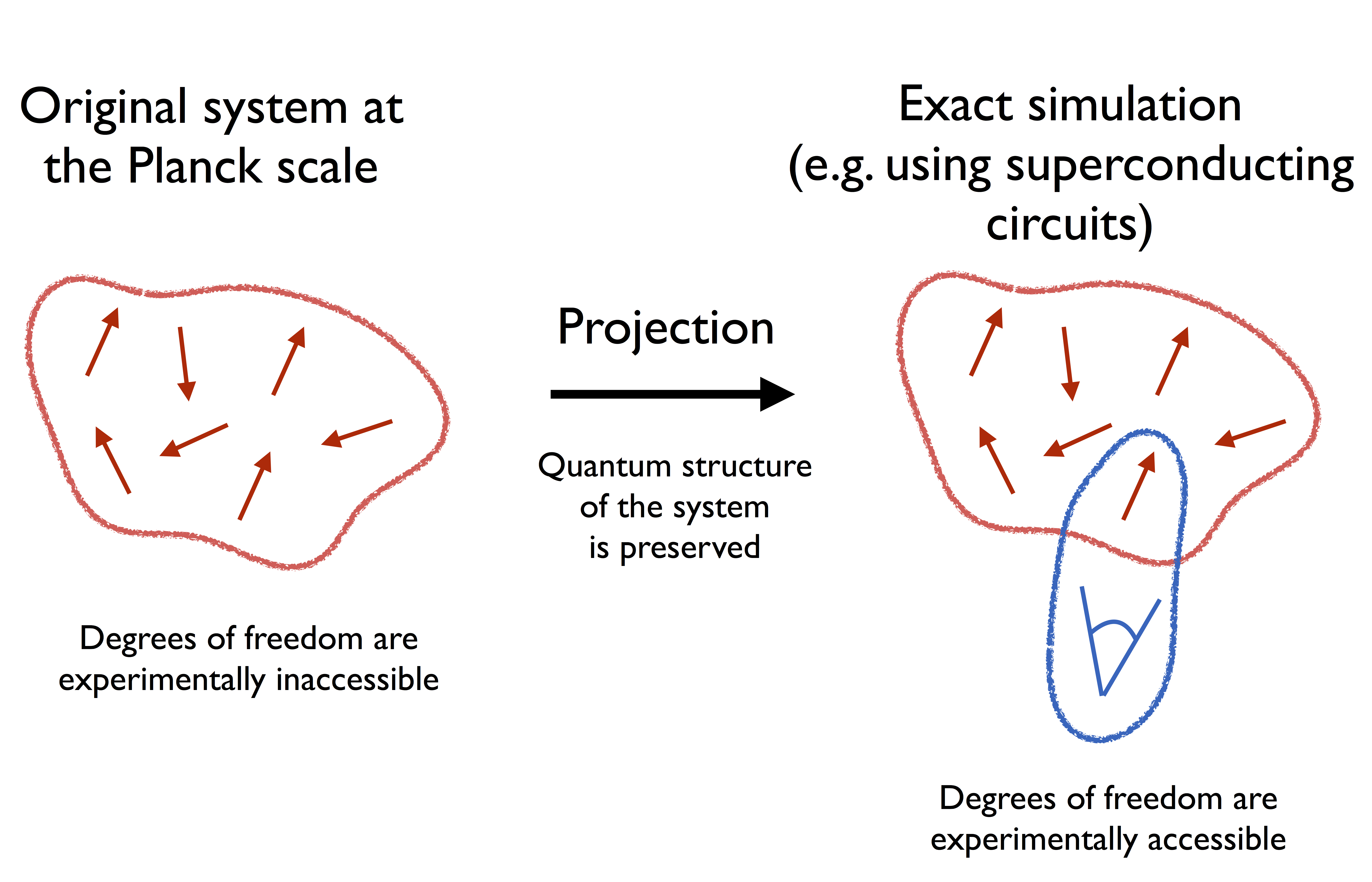
Figure 1: Pictorial presentation of the relation between the original quantum system defined at the Planck scales and its exact simulation. The exact simulation is performed with the use of projection of the original quantum system onto the architecture of a quantum computer. In contrast to the Planck scale system, measurements of the quantum degrees of freedom can be performed at the level of the quantum simulation.

On the other hand, concrete examples of theories describing elementary quantum gravitational degrees of freedom exist. One such approach is Loop Quantum Gravity (LQG) [3]. In LQG, background independent degrees of freedom can be defined and some predictions can be made [4]. Even if the degrees of freedom under consideration are experimentally not accessible one can think about their projection onto another physical realization which will imitate its quantum behavior (see Fig. 1). Assuming that quantum mechanics is valid at the Planck scale, from the perspective of quantum theory such systems can be considered as equivalent. The only difference are appropriately rescalled couplings adjusted to the physical nature of the simulator (built e.g. with the use of superconducting qubits). Such projection of one quantum system into its equivalent imitation allows to perform what we previously called exact simulations. As we already mentioned, the quantum simulations are very different from what we usually consider as physical simulations, where for instance a given differential equation is discretized and then implemented on a computer with the use of appropriate algorithms. In contrast, in the case of exact simulations one actually does experiments on a quantum system which is defined as being equivalent (from the view point of quantum mechanics) to a part (or a whole) of the original quantum system.

The aim of the is article is to investigate a possibility of performing exact quantum simulations of the spin networks states which are used to construct Hilbert space of LQG approach to quantum gravity. We are interested in application of existing technology, therefore our focus is on the only commercially available quantum computer at the moment, namely the D-Wave machine which implements the so-called quantum annealing algorithm.

Furthermore, we are considering conceptual issues related with the possibility of simulating Loop Quantum Gravity based on the considered fixed graph case. Specifically, implementation of the scalar constraint is analyzed and a toy model of such a procedure is presented. We finish with an outlook of the next steps to be done in the research direction initiated in this article.

Worth mentioning here is that the idea of employing the spin networks states in quantum computations already appeared in the literature (see Refs. [5, 6, 7]). However, the potential of application of spin networks for the purpose of universal quantum data processing was considered only. Up to the best of our knowledge the issue of relating spin networks with adiabatic quantum computations was not considered before. Furthermore, while this article was in the final stage of preparation a study in which a LQG spin network is implemented on a molecular quantum simulator appeared. In the article a simulation of quantum fluctuations of a 5-node spin network in the kinematical regime was performed [8]. Here, we will consider the same type of spin network in Sec. 4 in the context of solving a prototype scalar constraint with the use of adiabatic quantum computations.

2 Adiabatic Quantum Computing

The last years have brought a significant progress in the development of quantum computing technologies [9]. First quantum computers have been commercialized and made available in a cloud or as an independent hardware units. In both cases the currently most advanced commercial technologies were possible to achieve thanks to the development of superconducting quantum circuits [10]. In particular, the IBM Q universal quantum computer built with the use of 5 and 20 superconducting qubits has been developed. However, from the point of view of exact simulations discussed in the Introduction, another type of quantum computer seems to be more suitable to use - namely the adiabatic quantum computer [11].

The adiabatic quantum computers, in contrast to the universal ones, are designed to solve a specific problem of finding minimum of a Hamiltonian $H_{I}$ of a coupled system of qubits (spins). In the process of finding the minimum of $H_{I}$ one employs a time dependent Hamiltonian in the form

$$H(\lambda)=(1-\lambda)H_{B}+\lambda H_{I},$$ (1)

where $H_{B}$ is so-called base Hamiltonian which is characterized by a simple and easy to prepare ground state. In practice, the base Hamiltonian is often equal to $H_{B}=\sum_{i}\sigma^{x}_{i}$, such that the ground state corresponds to the alignment of spins in the $x$ direction. Then, the value of $\lambda$ is changed adiabatically from $\lambda=0$ to $\lambda=1$, such that while the system is initially in non-degenerate ground state it will remain in a ground state. Therefore, if the process is done correctly, the system ends up in the minimum of the Hamiltonian $H_{I}$. The process of transition from $\lambda=0$ to $\lambda=1$ involves quantum tunneling and is called quantum annealing. The characteristic time scales which preserve adiabaticity are dependent on what kind of $H_{I}$ Hamiltonian is considered. The issue is closely related with the efficiency of quantum annealing based algorithms with respect to the classical ones (see Ref. [1] for discussion of this subject).

In practical implementations the most considered form of $H_{I}$ corresponds to the Ising problem:

$$H_{I}=\sum_{<i,j>}b_{ij}\sigma^{z}_{i}\sigma^{z}_{i}+\sum_{i}h_{i}\sigma^{z}_{i},$$ (2)

where $b_{ij}$ are coupling between spins and $h_{i}$ quantifies interactions of spins with external magnetic field. The summation $<i,j>$ is defined such that it does not repeat over pairs. The values of couplings define the problem to be solved while readout of $z$ components of the spins in the final state provides an outcome of the quantum computation (simulation).

From the mathematical viewpoint, the class of problems which can be solved in that way is the so-called Quadratic Unconstrained Binary Optimization (QUBO) which typically is of the NP hard type. This is because, when we look a the problem from the classical perspective by measuring the orientations of spins along the $z$-axis, the two values of $\sigma^{z}_{i}\rightarrow s_{i}\in\{-1,1\}$ are allowed. In consequence, for the system of $N$ classical spins, there are $2^{N}$ configurations to be explored. Therefore, in general, finding a ground state requires exponential growth of time with the number of spins ($N$).

The physical implementation of the QUBO problem with the use of quantum annealing procedure is provided by the D-Wave machine. In this realization, the spins (qubits) are created with the use of superconducting circuits in the form of CC JJ RF-SQUIDs [12] built with the use of Josephson junctions composed of Niobium in superconducting state. The qubit base states are defined employing two different orientations of quantum of magnetic flux across the superconducting circuit. Interactions between the qubits are introduced by SQUID (superconducting quantum interference device) based circuits called couplers, which introduce the $b_{ij}\sigma^{z}_{i}\sigma^{z}_{i}$ factors in the Hamiltonian (2). Furthermore, with the use of external magnetic fluxes the values of parameters $h_{i}$ can be controlled. However, not all values of $b_{ij}$ and $h_{i}$ are allowed but only some fractional values from the range $[-1,1]$. The readout of the final quantum states of qubits is performed with the use of sensitive magnetometers built with the use of SQUIDs.

In the D-Wave quantum annealer, the superconducting qubits $q_{i}$ are arranged into 8-qubit blocks forming the so-called Chimera architecture. Each block has 16 couplings between 8 spins. Therefore, not all qubits are coupled. The topology of couplings between qubits in a single block is presented in Fig. 2. In the so far most advanced version of the D-Wave machine (the D-Wave 2000) the 8-qubit blocks form a 16x16 matrix (256 blocks in total) leading to 2048 qubits.

a)

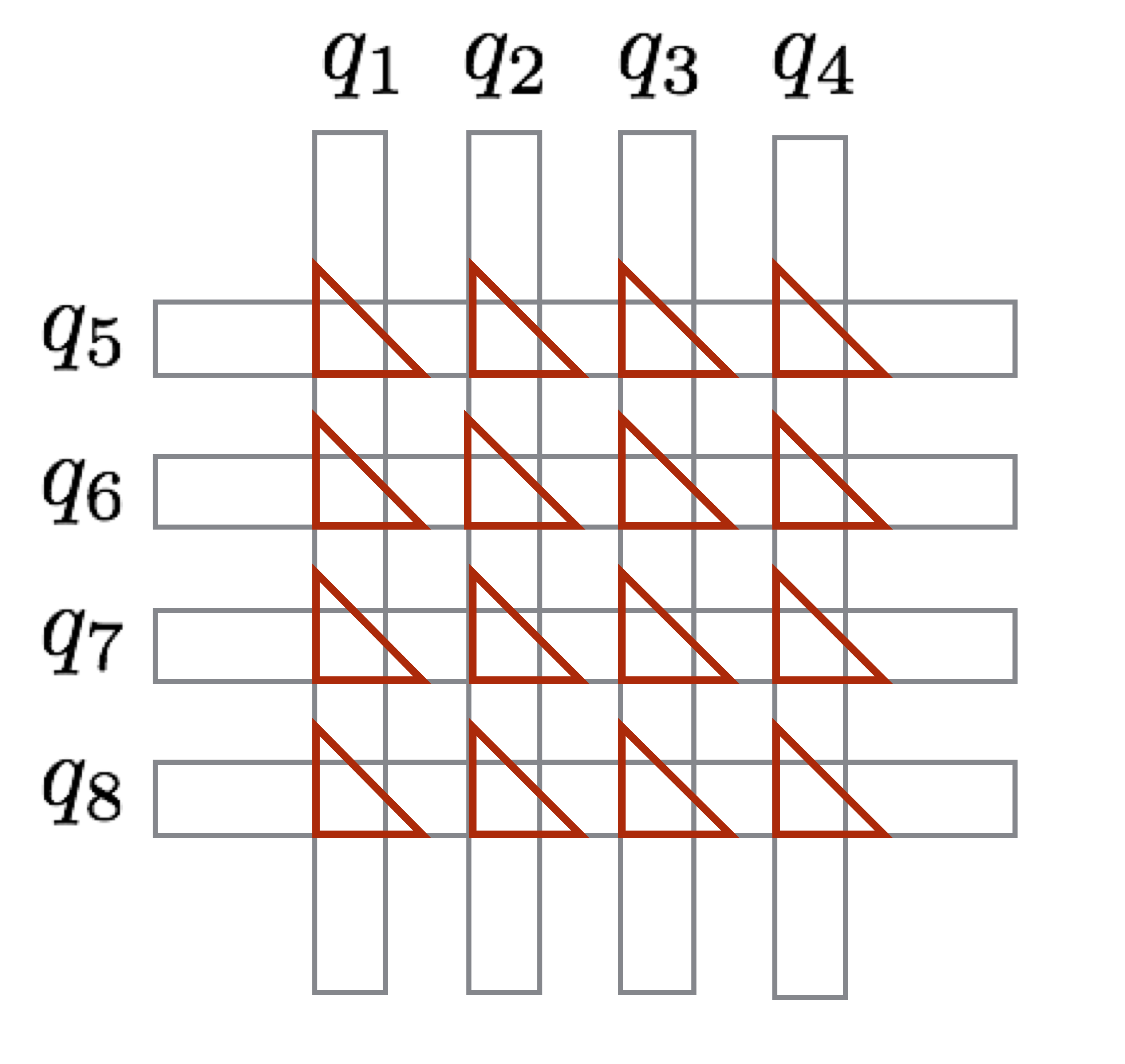
b)

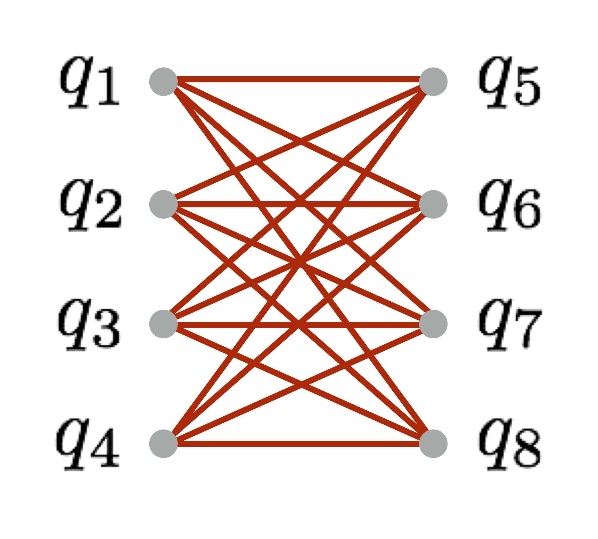
c)

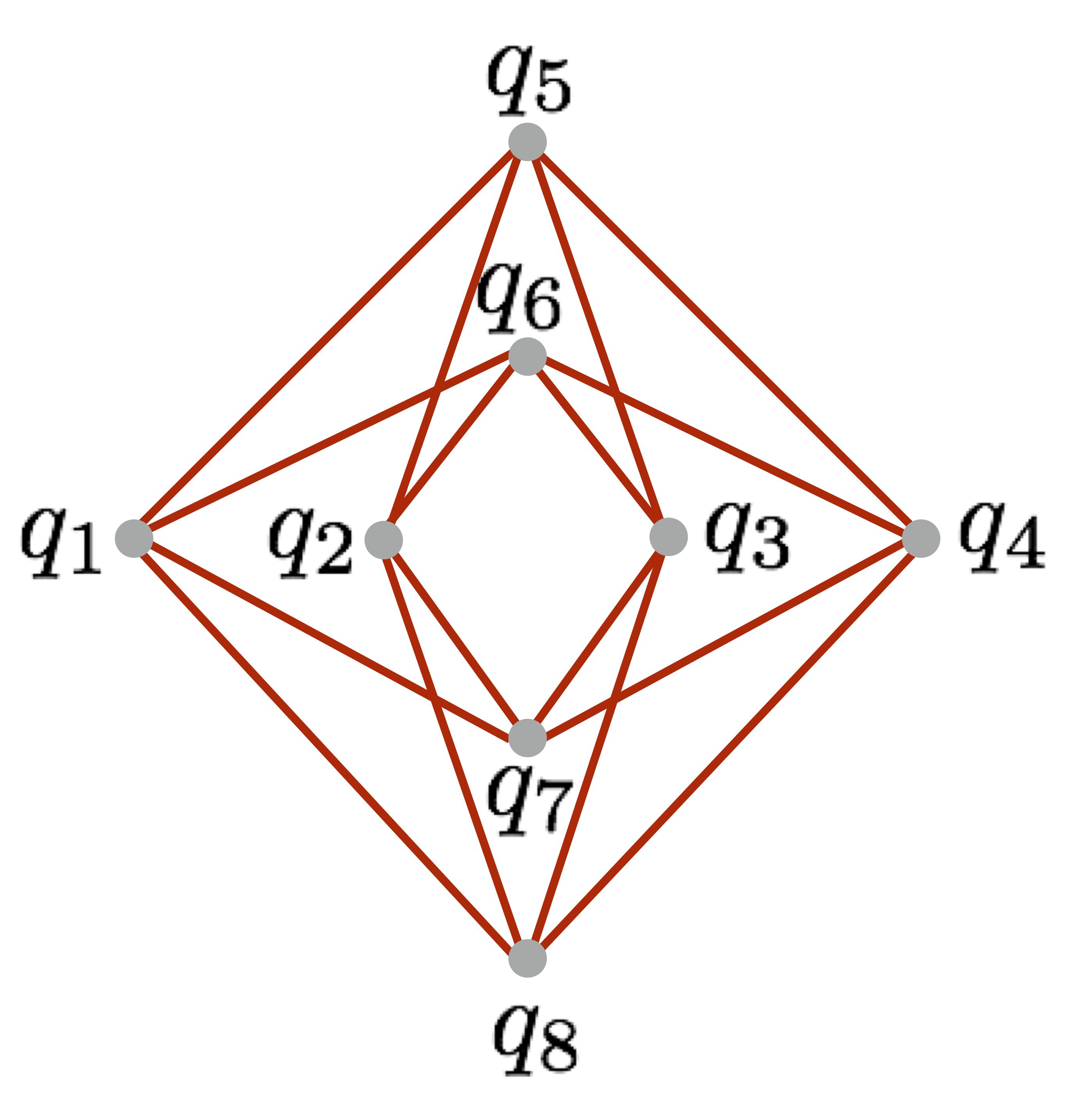
Figure 2: Three different representations of the structure of couplings between eight $q_{i}$ qubits forming an elementary block of the D-Wave processor: a) The physical representation of quibits as closed superconducting loops. The couplers between the qubits are represented by triangles. b) The Chimera graph structure of couplings between the eight qubits. c) Representation of a single block which is useful when interconnections in the array of blocks are considered.

3 Spin Networks

Let us now move to the subject of spin networks. We will start with a brief overview of how spin networks appear in the Loop Quantum Gravity approach to quantum gravity. Then we will introduce a class of spin networks which is possible to implement on Chimera architecture of a quantum processor.

The fundamental elements of Loop Quantum Gravity approach to quantum gravity are holonomies of Ashtekar connection $A\in su(2)$ along some curve $e(\lambda)$ with $\lambda\in[0,1]$:

$$h[A,e]=\mathcal{P}e^{\int_{e}A}.$$ (3)

Performing gauge transformations, generated by the so-called Gauss constraint, the Ashtekar connection transforms as $A\rightarrow A_{g}=g^{-1}dg+g^{-1}Ag$. The corresponding transformation of holonomy is $h[A,e]\rightarrow h[A_{g},e]=g(e(0))h[A,e]g(e(1))^{-1}$. The fact that the transformations of holonomies contribute only at the boundaries of $e$ implies that gauge invariant objects are provided by the Wilson loops $W[A,e]:={\rm tr}\left(h[A,e]\right)$.

The key idea behind LQG is to built a Hilbert space of the theory out of the Wilson loops. However, such basis is in general over-complete. A solution to the problem comes from construction of spin-networks which are certain linear combination of products of the Wilson loops [13]. Such approach guarantees that both the Gauss constraint (ensuring local gauge invariance) is satisfied by the base states and the Hilbert space is complete. Furthermore, by introducing equivalence relation between topologically equivalent spin networks, the so-called diffeomorphism constraint can be satisfied. There is finally a scalar constraint which has to be satisfied by physical states. In this section we will focus on the spin networks states satisfying both the Gauss and diffeomorphism constraint. We will came back to the issue of satisfying the scalar constraint (with the use of adiabatic quantum computing) in the next section.

The spin network is formally a graph composed of edges $E$ and nodes $N$ with spin labels at the edges and so-called intertwiners at the nodes. The spin labels correspond to irreducible representations of the $SU(2)$ group such that triangle inequalities (reflecting the Gauss constraint) are satisfied at the nodes. The intertwiners correspond to invariant subspaces at the nodes, which we will discuss in more details below.

In Fig. 3 we present an exemplary spin network composed of 3-valent and 4-valent nodes. An important feature of the nodes is that 3-valent nodes do not carry a volume element while 4-valent nodes and higher valent nodes are associated with 3-volume (in the sense that eigenvalues of the volume operator in such a state are non-vanishing).

a)

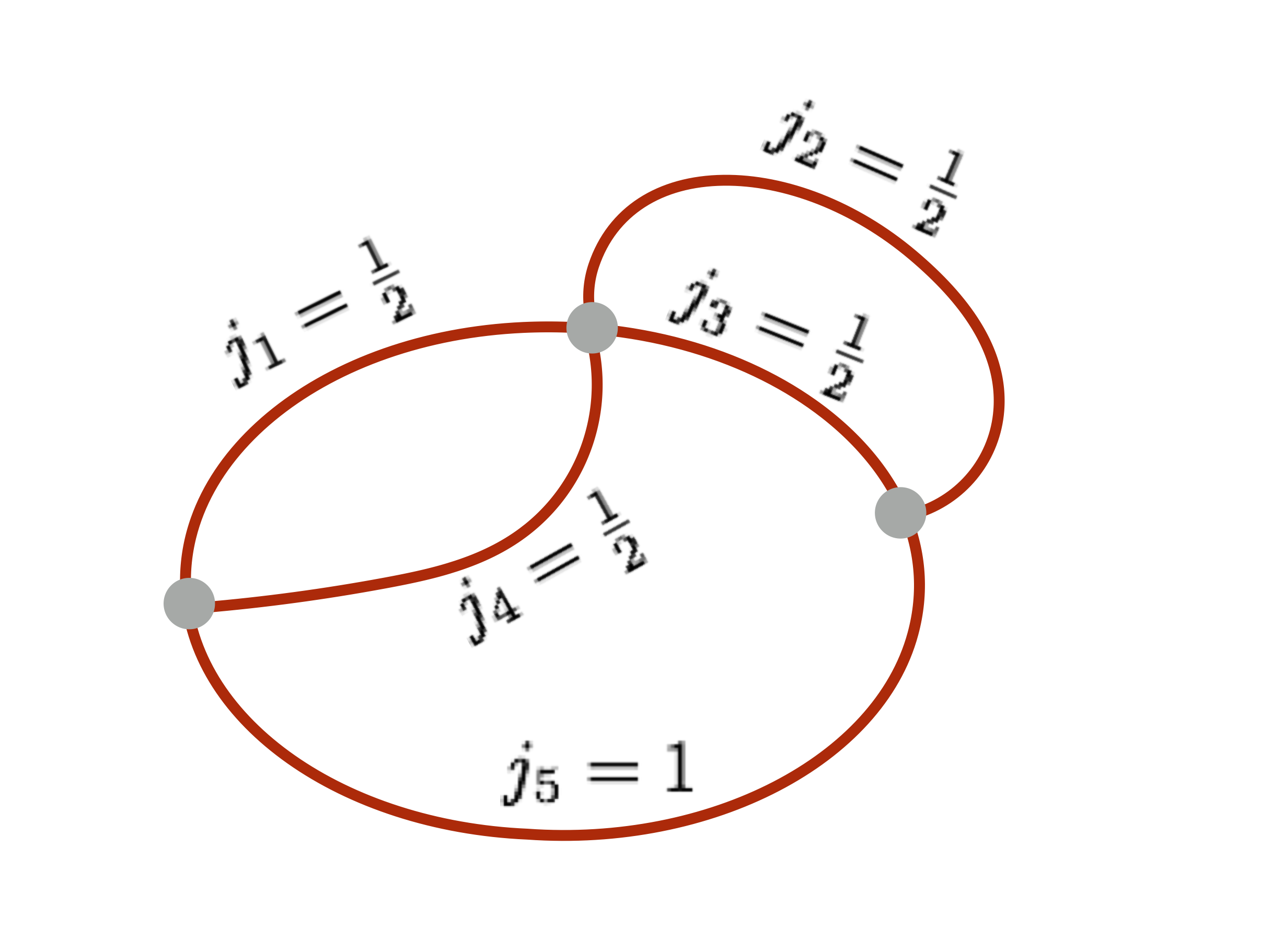
b)

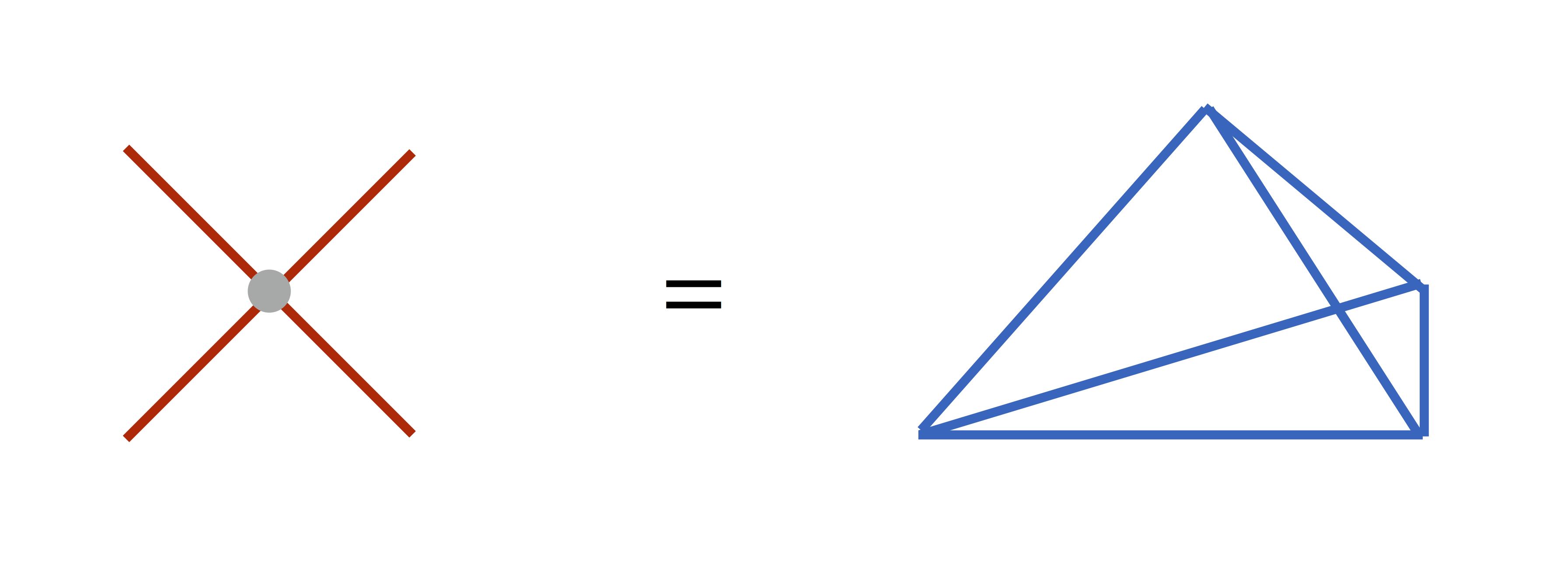
Figure 3: a) An exemplary spin network. b) In the geometric picture the 4-valent node is dual to a tetrahedron (3-simplex).

The special case of the nodes are 4-valent nodes which in the geometric picture are dual to a tetrahedra (3-simplexes). One can imagine that the vertex is located in the center of the tetrahedra while each of the associated links intersects with one of the surfaces (see block b) in Fig. 3).

In this article we are considering the case of spin networks composed only out of 4-valent vertices and spin labels corresponding to fundamental representations of the $SU(2)$ group i.e. $j=1/2$. The reason for that is that in such a case the Hilbert space at each vertex is a tensor product of four 1/2 spins which can be decomposed into irreducible representations in the following way:

$$H_{1/2}\otimes H_{1/2}\otimes H_{1/2}\otimes H_{1/2}=H_{0}\oplus H_{0}\oplus 3H_{1}\oplus H_{2}.$$ (4)

There are, therefore, two possibilities in which the spins can add up to zero. In consequence, the invariant subspace for such a vertex is two dimensional:

$${\rm dim\ Inv}(H_{1/2}\otimes H_{1/2}\otimes H_{1/2}\otimes H_{1/2})=2.$$ (5)

We associate the two dimensional invariant space with the qubit space. The nature of the qubit associated with the 4-vertex under consideration is graphically presented in Fig. 4.

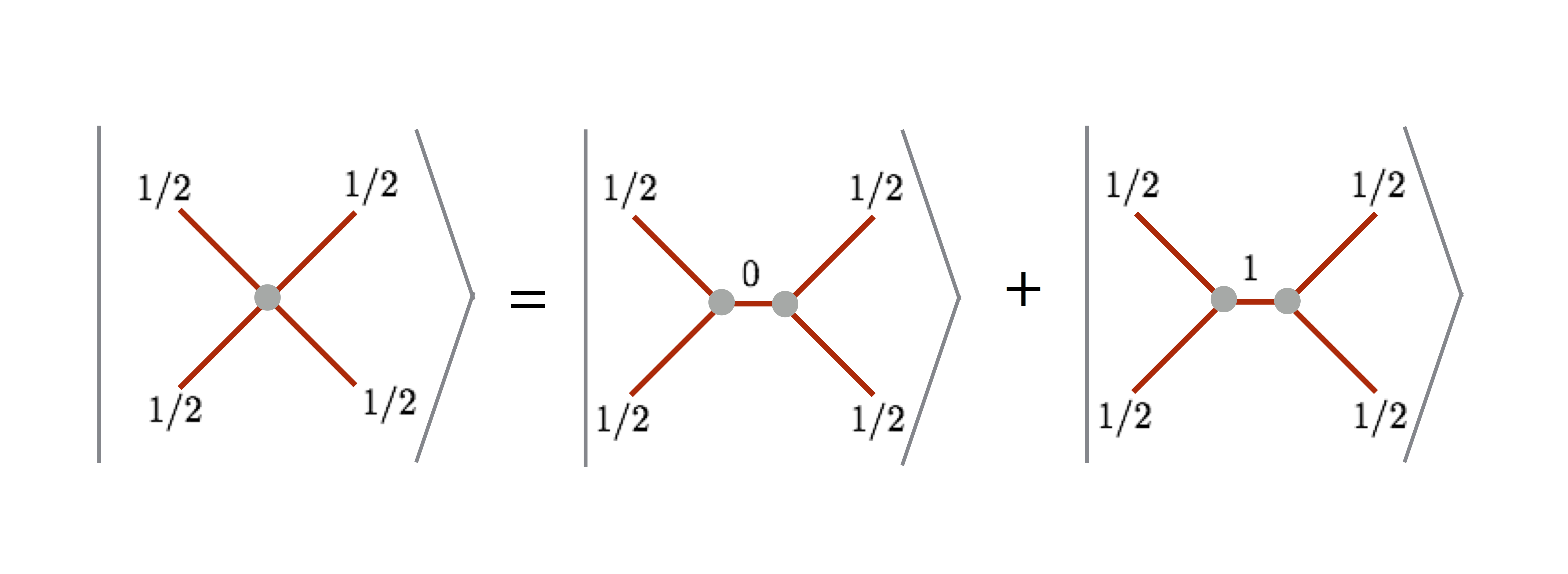
Figure 4: The 4-valent node with spin labels equal to $j=1/2$ corresponds to superposition of two graphs each with the different value of intertwiner. In this article, the two dimensional intertwiner space is associated with the qubit Hilbert space.

Worth mentioning here is that there is a freedom of choice of channel in which recoupling of spin labels at the vertex is performed. In particular, in the $s$ channel the base states can be expressed in terms of the four $1/2$ spin base states ($|\uparrow\rangle$ and $|\downarrow\rangle$ ) as follows [14]:

$$|0_{s}\rangle = \frac{1}{2}\left(|\uparrow\downarrow\uparrow\downarrow\rangle+|\downarrow\uparrow\downarrow\uparrow\rangle-|\uparrow\downarrow\downarrow\uparrow\rangle-|\downarrow\uparrow\uparrow\downarrow\rangle\right)$$

$$|1_{s}\rangle = \frac{1}{\sqrt{3}}\left(|\uparrow\uparrow\downarrow\downarrow\rangle+|\downarrow\downarrow\uparrow\uparrow\rangle-\frac{|\uparrow\downarrow\uparrow\downarrow\rangle+|\downarrow\uparrow\downarrow\uparrow\rangle+|\uparrow\downarrow\downarrow\uparrow\rangle+|\downarrow\uparrow\uparrow\downarrow\rangle}{2}\right).$$

Then, it is convenient to construct our qubit states such that they are eigenvectors of the volume operator $\hat{V}$ (see e.g. Ref. [14] for details). This can be achieved by considering the following superpositions of the states (LABEL:schannel):

$$|1\rangle = \frac{1}{\sqrt{2}}\left(|0_{s}\rangle-i|1_{s}\rangle\right),$$ (7)

$$|0\rangle = \frac{1}{\sqrt{2}}\left(|0_{s}\rangle+i|1_{s}\rangle\right),$$ (8)

such that $\hat{V}|1\rangle=+V_{0}|1\rangle$ and $\hat{V}|0\rangle=-V_{0}|0\rangle$, where $V_{0}=\frac{\sqrt{3}}{4}l^{3}_{Pl}$ is the absolute value of the quantum of volume. The $|1\rangle$ and $|0\rangle$ are the qubit states that we refer to in the rest of this article. From the geometrical point of view, the two base states are associated with two orientations of the elementary 3D symplex of space. Worth stressing is that the volume can be either positive (for $|1\rangle$) or negative (for $|0\rangle$). Therefore, in LQG the elementary volume can contribute with both signs. However, it is expected that in the semiclassical limit one of the contribution will dominate such that the net configuration will be characterized by non-vanishing volume.

Having the definition of a qubit one can try to consider different spin network topologies which are possible to implement directly with the use of Chimera architecture. In Fig. 5 we present connected spin networks with the number of nodes equal to $N=2,3$ and $4$ which can be directly embedded into the Chimera graph.

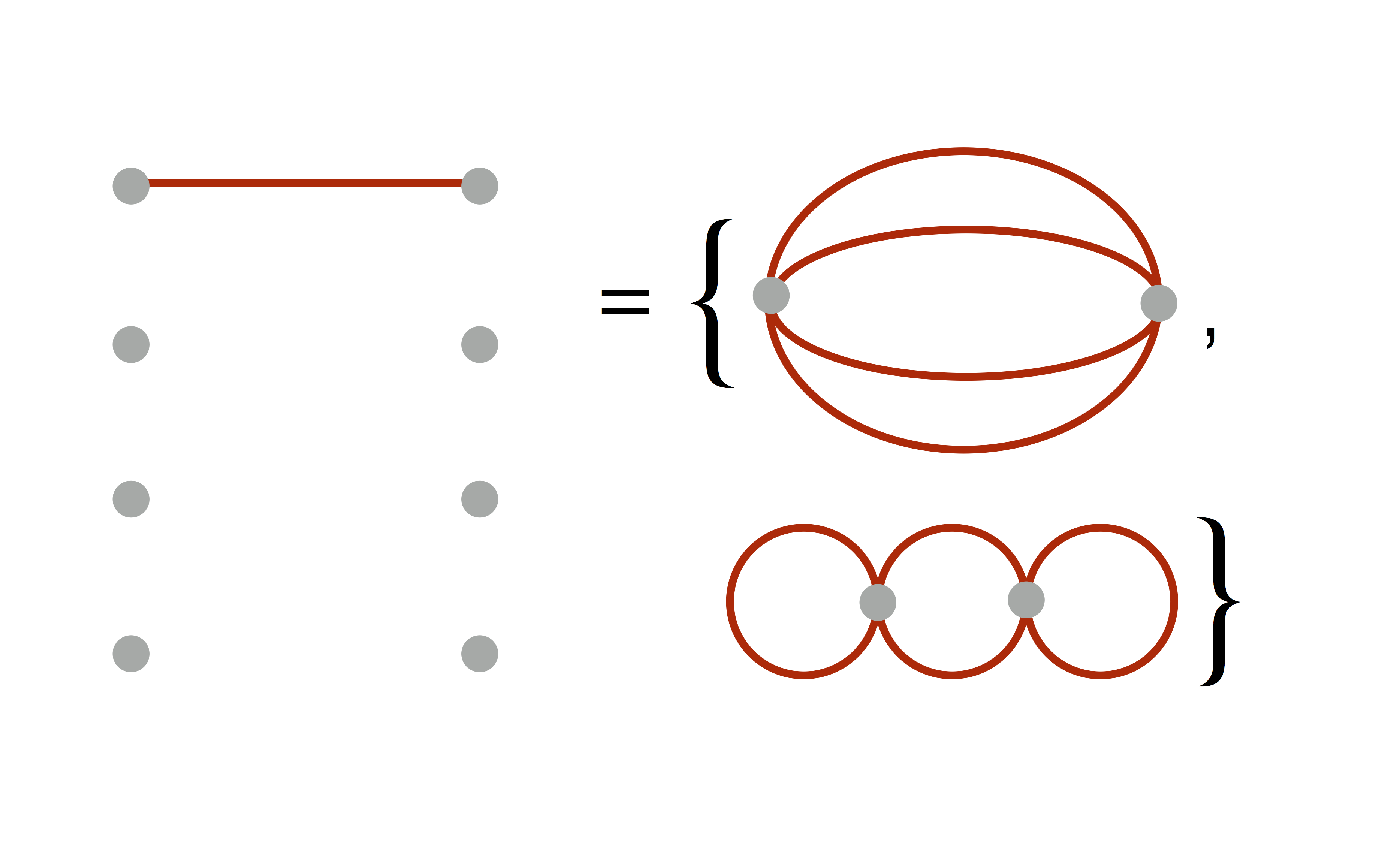
a)	b)
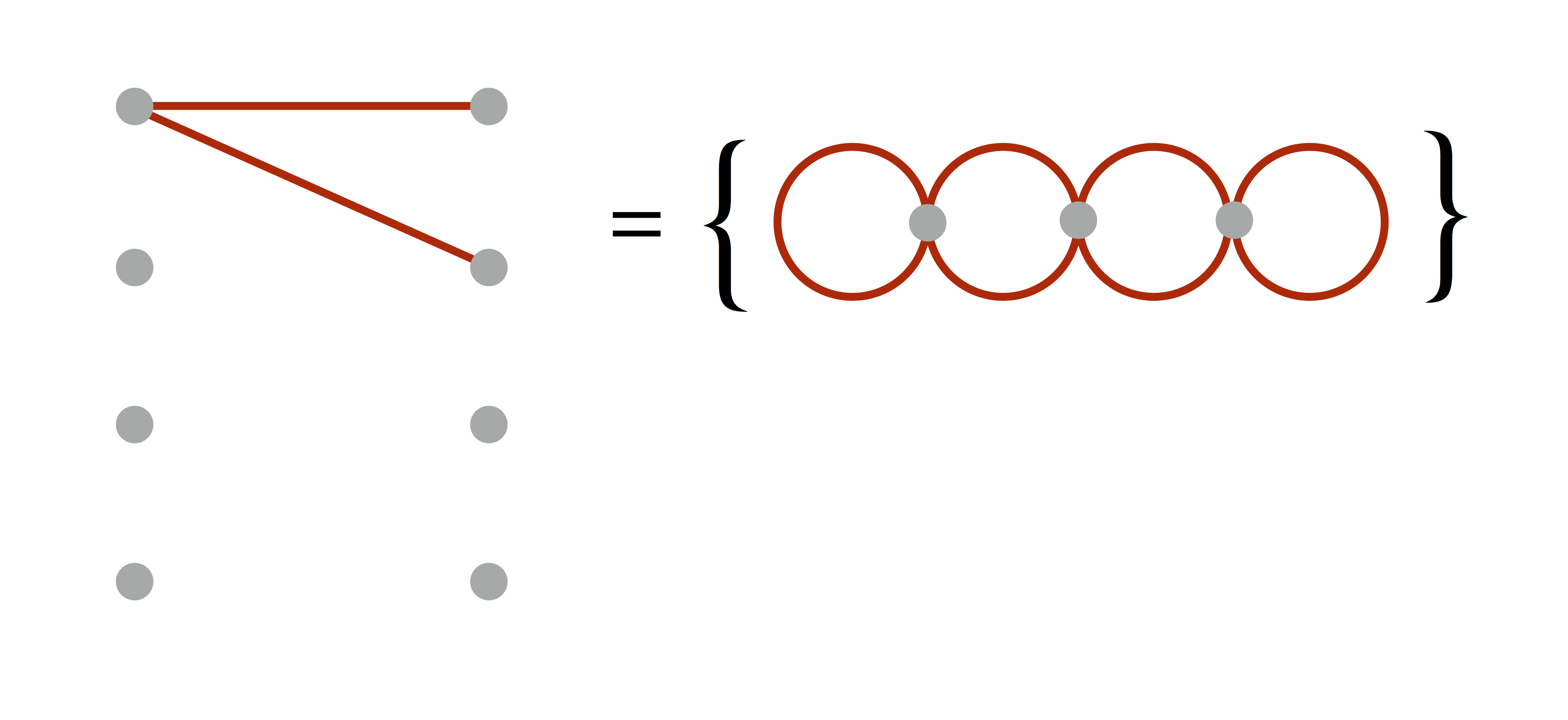
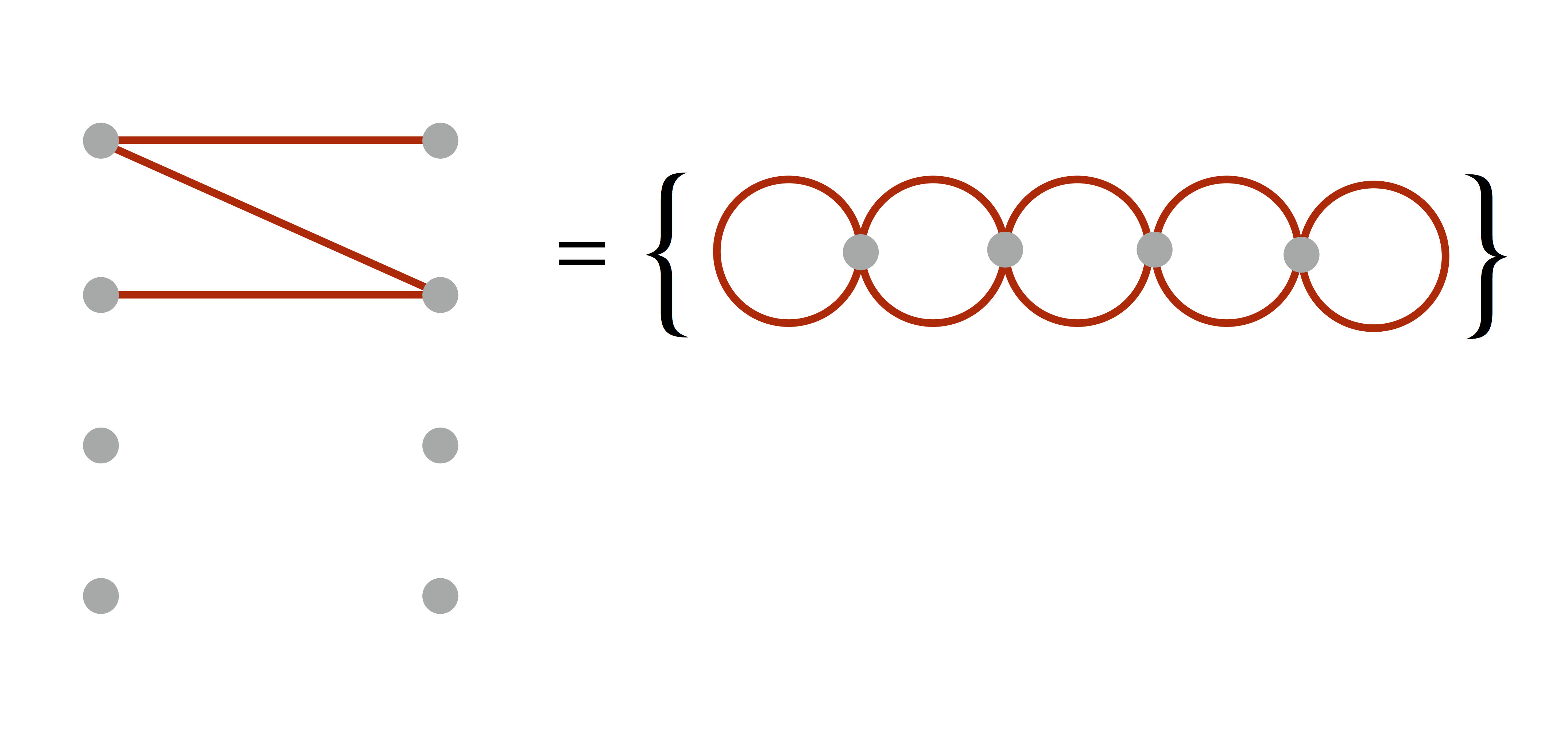
c)	d)

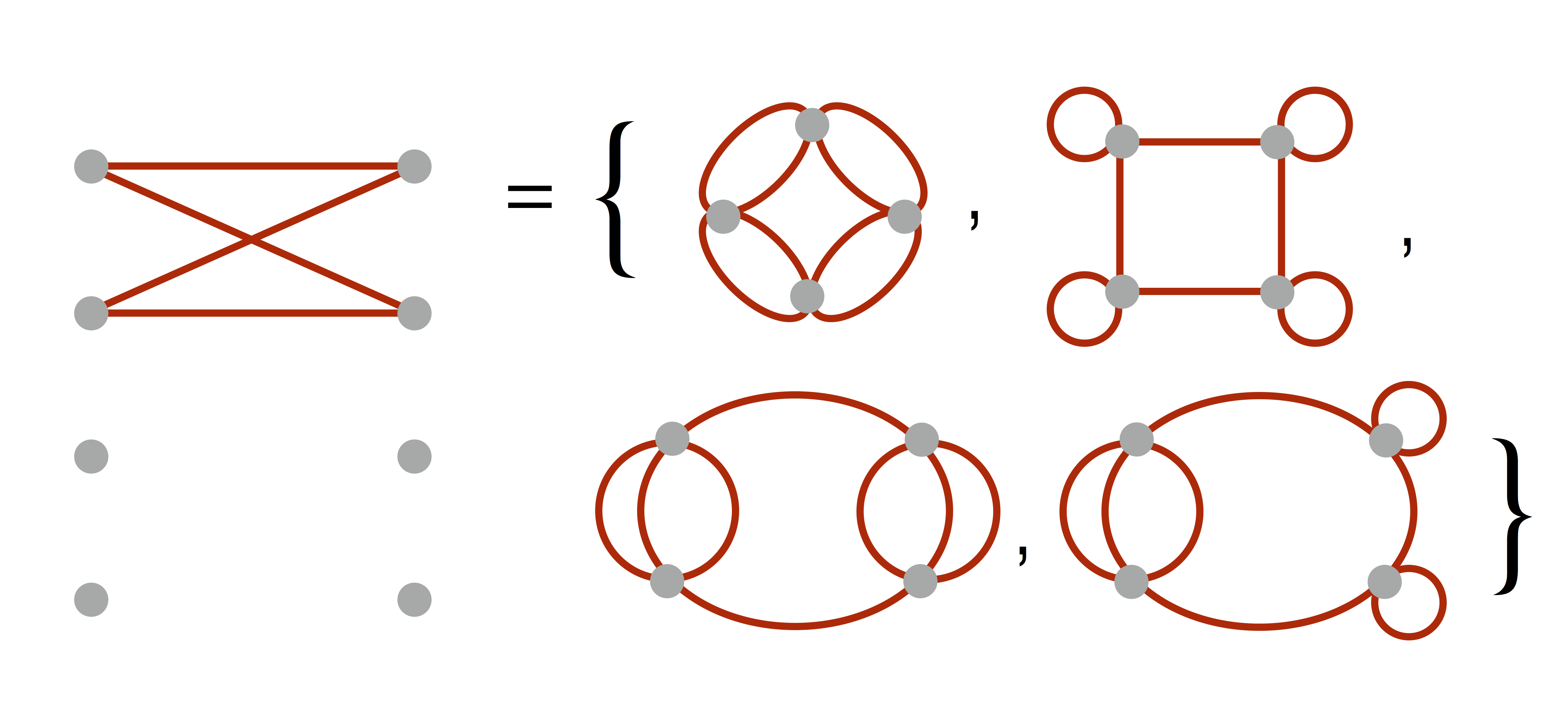
Figure 5: Connected spin networks compatible with the Chimera architecture: a) $N=2$, b) $N=3$, c) $N=4$, d) $N=4$.

A single coupling between the qubits in the quantum processor architecture can be associated with one or more links in the corresponding spin network. The difference between connections can be further encoded in the strength of the couplers. In particular in the case a) in Fig. 5 there are two possible 4-valent spin networks which can be associated with two coupled qubits. Relating a single coupler with a single link in the spin network is generically not possible. In the case of 4-valent nodes and a single block of D-Wave processor the only possibility is given by the configuration represented in blocks b) and c) in Fig. 2. The situation corresponds to a spin network with $N=8$ qubits and $E=16$ edges forming the Chimera graph.

As one can notice the structure of Chimera architecture imposes significant restrictions on the possible associated spin network topologies. In particular, it is not possible to implement a “triangular” $N=3$ spin network directly with the use of elementary qubits. In order to go beyond restrictions of the Chimera architecture one can consider effective qubits (chain qubits) composed from two or more spins. If the coupling between the qubits is sufficiently negative then the qubits will have tendency to align in the same direction, which is preferred energetically. In such a case, measurements can be performed on one of the elementary qubits contributing to the chain while the remaining qubits can be considered as ancilla qubits.

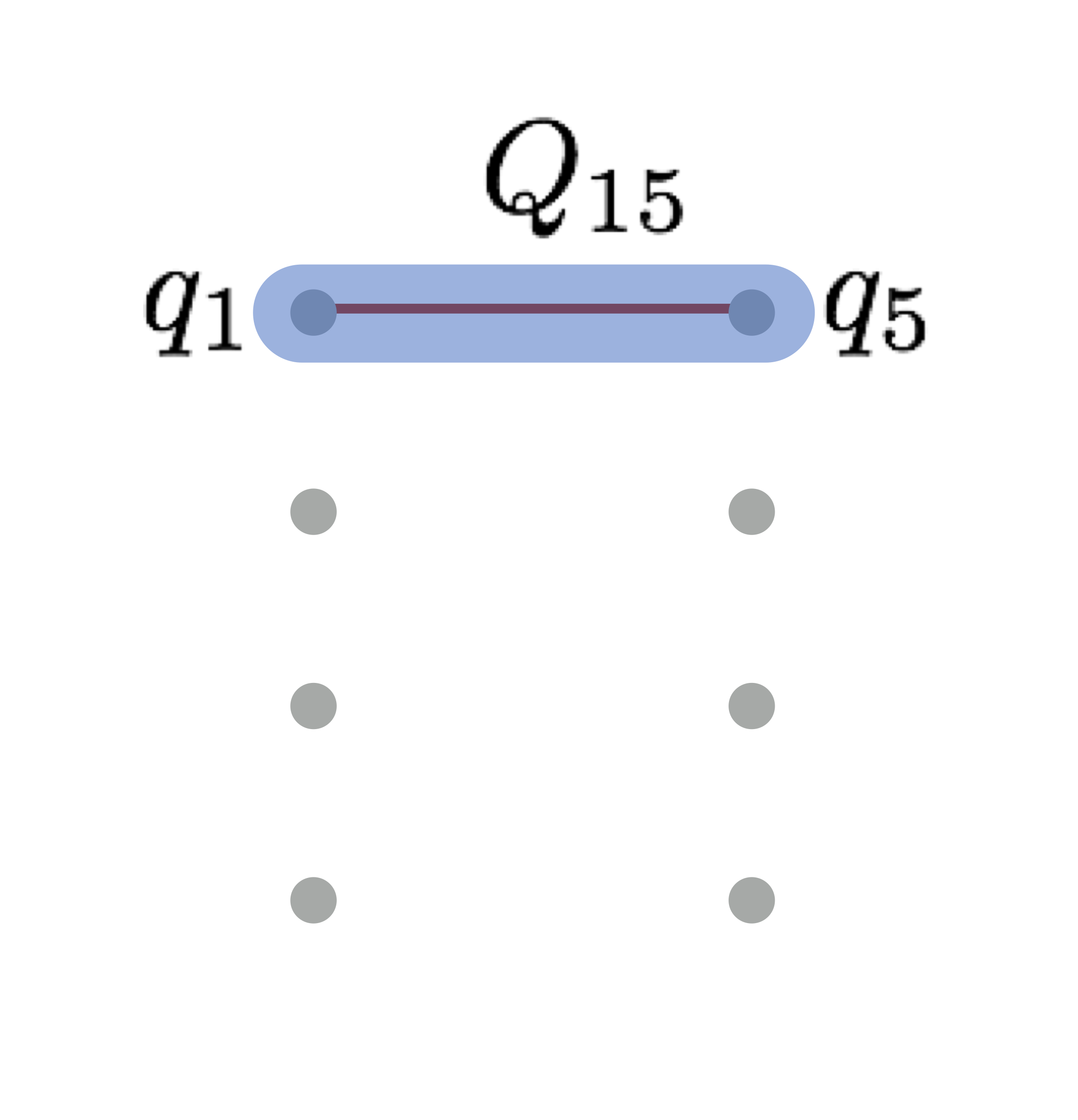
Figure 6: A chain qubit. If the $b_{15}$ coupling is sufficiently negative then the spins $q_{1}$ and $q_{5}$ will have tendency to align in the same direction.

With the use of chain qubits the dictionary of spin networks can be extended further. In particular, previously inaccessible spin networks for $N=3$ and $N=4$ can now be constructed (see Fig. 7).

a)

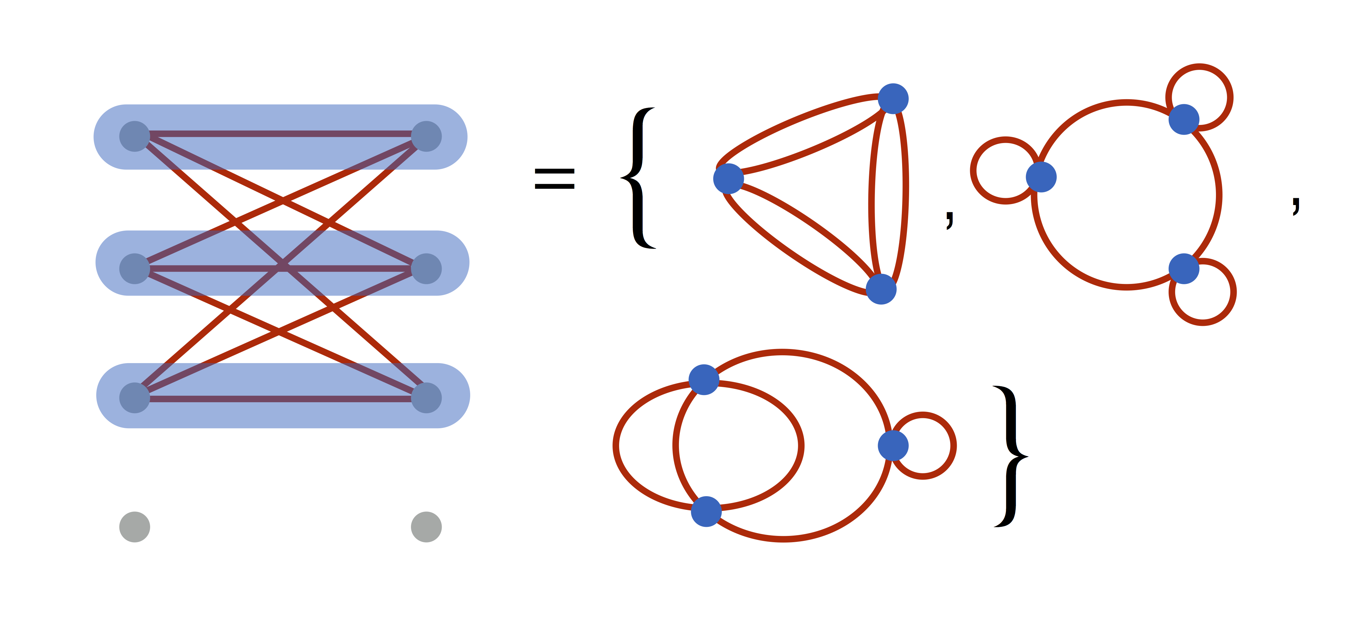
b)

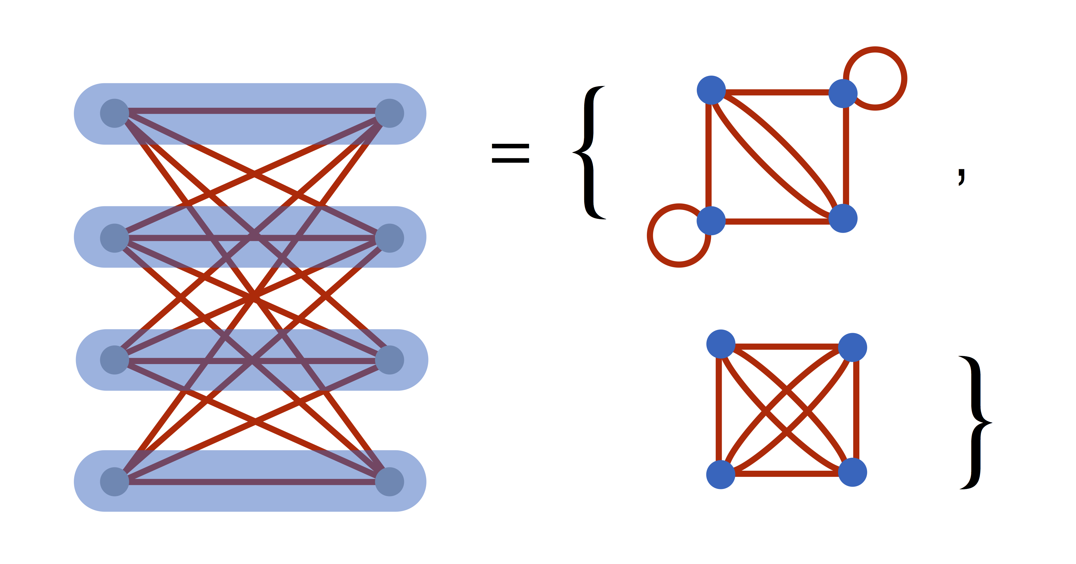
Figure 7: Connected spin networks compatible with Chimera architecture: a) $N=3$, b) $N=4$.

Worth stressing is that different types of effective qubits can be considerer and Fig. 7 represents only a one of many possible implementations of the spin networks under consideration.

A more extended example is a regular square lattice with the nearest neighbor connections.

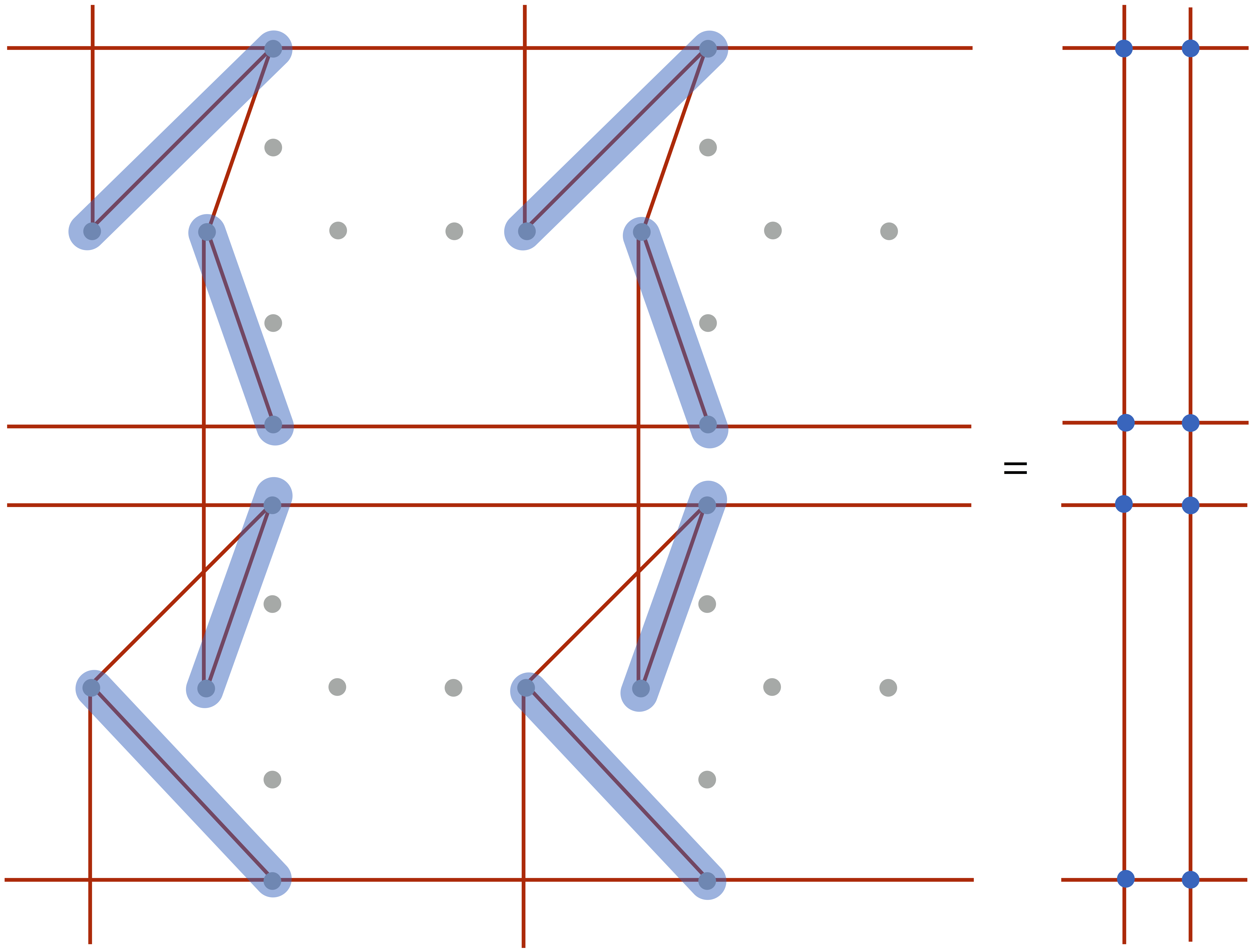
Figure 8: Regular lattice spin network embedded with the use of chain qubits. Here, four 8 qubit blocks of the D-Wave processor are used.

The regular lattice configuration enables to simulate a 2D Ising spin networks discussed in Ref. [14] which provide a toy model of extended quantum spacetime. Analysis of such configurations is especially interesting in the context of phase transitions and domains formation which may reflect emergence of semi-classical spacetime. We will come back to this issue in the next section. Furthermore, in the further studies it would be interesting to investigate if the 3D hexagonal type Ising spin network can also be embedded into the architecture of the D-Wave processor.

4 Simulation of Loop Quantum Gravity

The spin network states discussed in the previous sections satisfy the Gauss constraint. The diffeomorphism constraint can be imposed by considering equivalence classes under the action of diffeomorphism, which in practice means that we equate all graphs with the same topology.

Finally, the scalar (Hamiltonian) constraint remains, which is the most difficult one to satisfy. Finding solution to the Hamiltonian constraint in the 3+1 D can be perceived as the most difficult open problem in LQG [15].

Basically, the scalar constraints reflects the fact that the total energy of gravitational field is equal to zero. The scalar constraint is in general a graph changing operator making implementation of such a constraint a quite difficult task. However, the situations in which the graph structure is preserved by the action of the constraint may provide an intermediate step towards the solution of the full problem. Therefore, considering such a prototype graph non-changing scalar constraints is worth considering. The question is now whether adiabatic quantum computation may be useful here?

In order to answer to this question, let us observe that finding solutions to the classical constraint:

$$C\approx 0,$$ (9)

can be mapped into a problem of minimizing some Hamiltonian. Because the quantum annealing algorithm is just searching for minimum of the spin Hamiltonian (2), making use of adiabatic computations requires association of the minimum of the Hamiltonian with solution of the constraint (9). The simplest way to do it is to consider the Hamiltonian $H$ in the following form:

$$H\propto C^{2}.$$ (10)

In such a case the Hamiltonian is bounded from below and at the ground state the constrain (9) is naturally satisfied.

Solution of the constraint (9) allows to extract physical states and construct a physical phase space $\Gamma_{\rm phys}$ (or physical Hilbert space $H_{\rm phys}$) being a subset of kinematical phase space $\Gamma_{\rm kin}$. It is important to stress that the minimum energy states of the Hamiltonian (10) are just the physical states of the theory and they form $\Gamma_{\rm phys}$. If there is no additional matter content, the states represent also a vacuum gravitational field configuration, described by the prototype scalar (Hamiltonian) constraint under considerations. Worth mentioning here is that the auxilary Hamiltonian (10) can be in some sense considered as a Master Constraint introduced in LQG, being a square function of constraints (see Ref. [15]).

There are, however, technical limitations in implementation of the procedure proposed above. This is because, in the D-Wave machine only quadratic Hamiltonian functions are allowed. This implies that the scalar constraint cannot be of the higher than linear order in the spin variables. On the other hand, scalar constraints being of the higher that linear order in the spin variables is expected in the full LQG.

The most general type of the constraint that one consider in the context of D-Wave quantum computer is

$$C=\sum_{i=1}^{N}a_{i}s_{i}-c\approx 0,$$ (11)

with some parameters $a_{i},c\in\mathbb{R}$ and where $s_{i}\in\{-1,1\}$ are classical spin variables. Here, for the sake of simplicity we will consider the case with $a_{i}=1\ \forall i$, such that the prototype scalar constraint (11) takes the following form:

$$C=\sum_{i=1}^{N}s_{i}-c\approx 0,$$ (12)

with some parameter $c\in\{-N,-N+2,\dots,N-2,N\}$. By squaring (12) we obtain:

$$C^{2}=2\left(\sum_{<i,j>}^{N}s_{i}s_{j}+\sum_{i=1}^{N}(-c)s_{i}\right)+N+c^{2}.$$ (13)

Based on this one can propose that the Hamiltonian to be considered is

$$H=\frac{C^{2}-N-c^{2}}{2}=\sum_{<i,j>}^{N}s_{i}s_{j}+h\sum_{i=1}^{N}s_{i},$$ (14)

where $h=-c$. The obtained Hamiltonian corresponds to the QUBO problem with a complete graph and equal couplers between the qubits $(b_{ij}=1)$. In this model, the ground state (which corresponds to $C=0$) energy is:

$$H_{0}=-\frac{N+c^{2}}{2}.$$ (15)

There is one more important aspect illustrated by the model - a degeneracy of the ground state. Namely, there is, in general, no unique spin configurations which is minimizing the Hamiltonian (14). In the model under consideration, the vacuum degeneracy depends on both the values of $c$ and $N$. Given the $c$ and $N$, determination of the order of degeneracy is a combinatorial problem which can be reduced to finding a number of $(N+c)/2$ subset of a set composed of $N$ elements, which is given by binomial coefficient:

$$\left(\begin{array}[]{c}N\\ \frac{N+c}{2}\end{array}\right).$$ (16)

Then, for a fixed N the maximal degeneracy is obtained for the choices

$$c=2\lfloor N/2\rfloor-N\ \ \vee\ \ c=2\lceil N/2\rceil-N,$$ (17)

where $\lfloor x\rfloor$ and $\lceil x\rceil$ are floor and ceiling functions respectively. Based on this, the corresponding maximal degeneracy is equal to

$$\left(\begin{array}[]{c}N\\ \lfloor N/2\rfloor\end{array}\right)=\left(\begin{array}[]{c}N\\ \lceil N/2\rceil\end{array}\right).$$ (18)

The degeneracy is an important quantity because it corresponds to the number of physical states satisfying the constraint (12).

One can now make relation with the spin networks. For this purpose, let us recall that the spin Hamiltonian (14) corresponding to the constraint (12) describes a complete graph. Associating a spin coupler with a single link of the spin network one can conclude that for the 4-valent nodes under considerations the only complete spin network must have pentagram structure with $N=5$ nodes (see block a) in Fig. 9) .

Such spin network corresponds to geometry of a three-sphere. Furthermore, it turns out that introducing composite (chain) spins the pentagram spin network can be implemented with the use of two neighbor blocks of the D-Wave processor. There are various ways to do so. One of them is presented in block b) in Fig. 9, where the shadowed regions correspond to the effective qubits composed our of the elementary ones.

a)

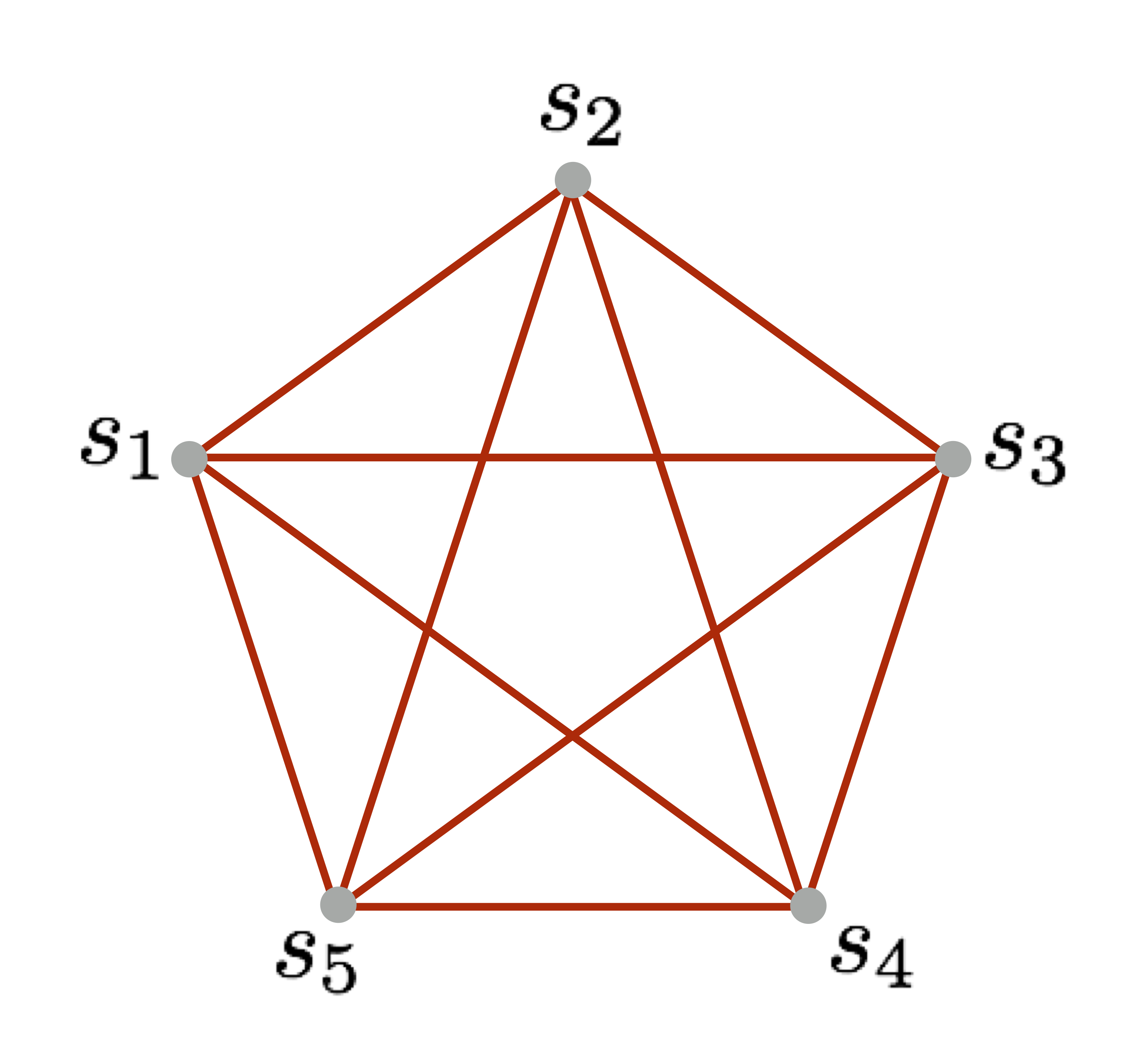
b)

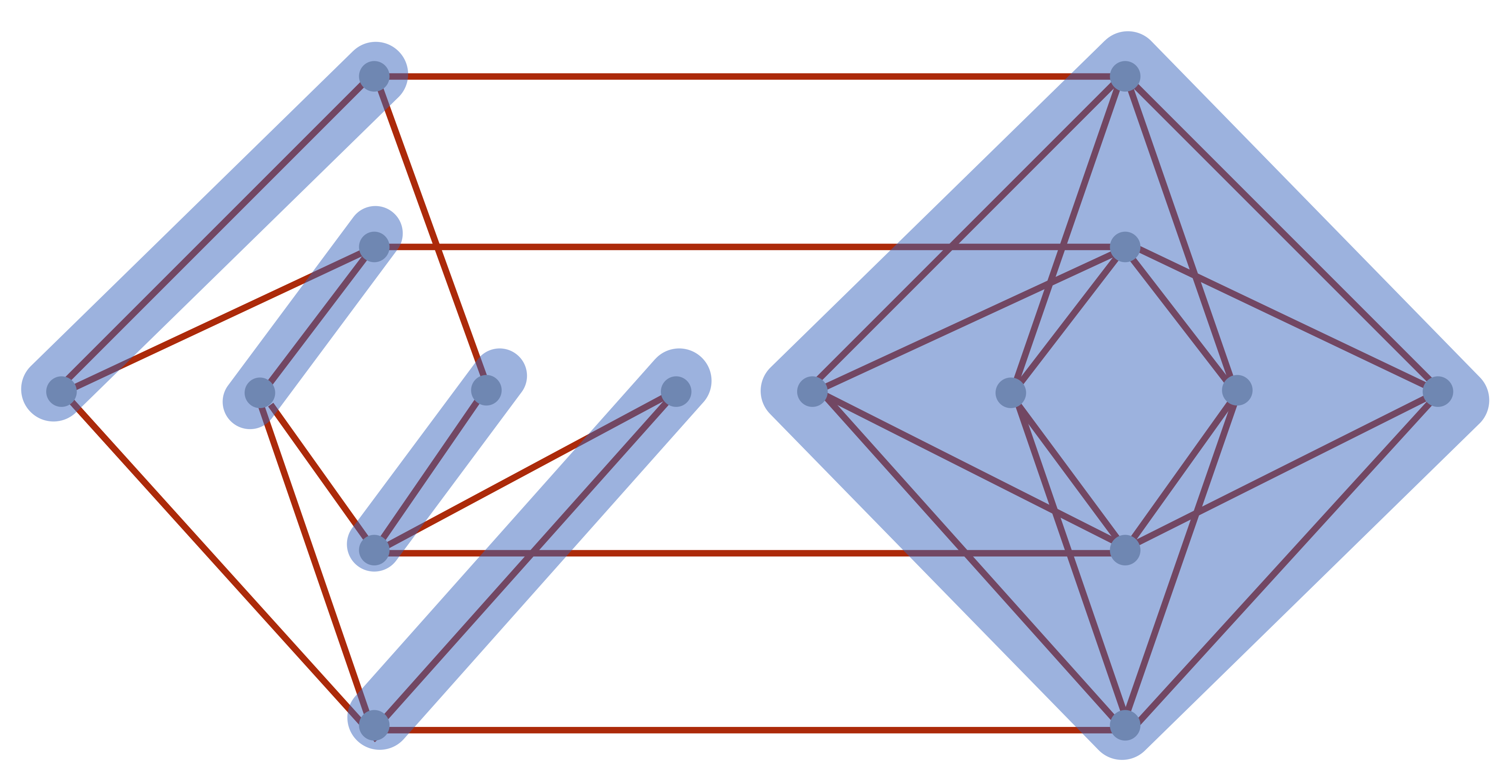
Figure 9: a) Pentagram spin network with $N=5$. Each link of the graph is labeled with $j=1/2$. The qubits (here modeled by the classical bits $s_{i}$) are defined at the nodes. b) An exemplary embedding of the pentagram spin network on the two neighbor blocks of the D-Wave processor. The shadowed regions represent collective (chain) qubits which correspond to the nodes of the spin network.

Finally, let us take a look at the energy landscape of the model. In Fig. 10 we plot energies corresponding to all of the spin configurations for $c=-1$.

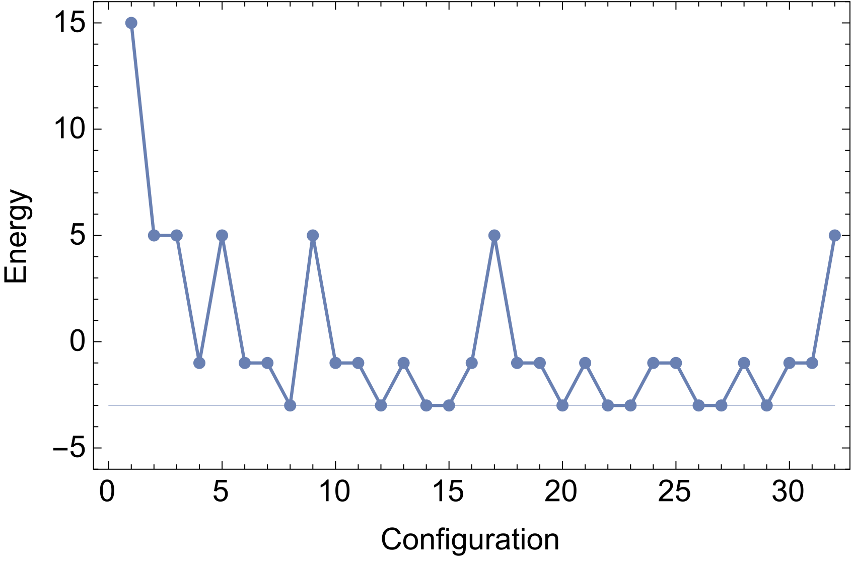
Figure 10: Energy landscape of the pentagram spin network with $N=5$ and $c=-1$. The ground state configurations satisfy the prototype scalar constraint (12) and span physical phase space $\Gamma_{\rm phys}$ of the model.

The total number of spin configurations corresponds to dimensionality of the kinematical space: ${\rm dim}\ \Gamma_{\rm kin}=2^{5}=32$. On the other hand, the degeneracy of the vacuum of (14) gives us dimensionality of the physical space ${\rm dim}\ \Gamma_{\rm phys}=\left(\begin{array}[]{c}5\\ \frac{5-1}{2}\end{array}\right)=10$ (here we used Eq. 16). The physical space is a subset of kinematical space $\Gamma_{\rm phys}\subset\Gamma_{\rm kin}$ as expected.

In order to extract all the physical states with the use of adiabatic quantum simulations the quantum annealing procedure has to be performed repeatedly. The outcome is a superposition of the ground states and the procedure of measurement should select the particular ground states in the independent runs. However, as discussed in Refs. [16, 17] the type of quantum annealing procedure used in the D-Wave quantum computers may not be suited to identify all degenerate ground states. The studies suggest that extension beyond the currently employed base Hamiltonians is needed to ensure that the ground state manifold is sampled properly. Otherwise, the probability of finding some of the possible ground states may be suppressed.

Assuming that the physical states are selected, analysis of fluctuations of various observables is possible to perform. In the case under consideration, one of the interesting possibilities would be to investigate volume fluctuations. As we mentioned, the base states corresponding to the 4-valent note qubits are eigenstates of the volume operator describing the same absolute volume but with the different signs. It is, however, expected that in the classical limit only one type of contributions will dominate such that averaged nonvanishing space volume will emerge. On the other hand, in a highly quantum state the positive and negative contributions can subtract one another leading to the lack of the notion of classical geometry. Analysis of correlations of the spins in the physical states could, therefore, say if e.g. domains of the same sign of volume form. If yes, that would be a sign of emergence of semi-classical spacetime. Furthermore, appearance the long range correlation would unavoidably allow to associate a notion of length scale to the spin network configurations. Such observation, would be a significant step towards reconstruction of classical spacetime directly from the spin network states.

5 Summary

The purpose of this article was to investigate a possibility of implementation of spin networks on the architecture of commercially accessible adiabatic quantum computers. In the studies, we focused our attention on spin networks with fixed spin labels ($j=1/2$) corresponding to fundamental representation of the $SU(2)$ group. In such a case the 4-valent nodes give rise to two dimensional intertwiner space which was associated with the qubit Hilbert space. In the geometric picture, the 4-valent nodes of spin network are dual to the 3D simplices and the qubit bases states represent different orientations of a 3-simplex.

We have shown that in the considered case it is possible to define spin networks on architecture of the D-Wave quantum processor. However, due to topological restrictions of the Chimera graph not all spin networks are possible to implement with the use of elementary qubits. However, some obstacles can be overcame by introducing effective (chain) qubits composed our of two or more elementary qubits. Such effective qubits allow to implement e.g. regular 2D square lattice topology of the nearest neighbor type of interaction Ising model.

Furthermore, we proposed a method of solving scalar (Hamiltonian) constraints with the use of quantum annealing. We have shown that in the case of D-Wave quantum annealer, a prototype constraint being a linear function of qubit variables is possible to solve. The solutions of the constraint (i.e. physical states) are obtained at the vacuum of an appropriate Ising type Hamiltonian. The procedure has been theoretically demonstrated for the pentagram spin network, which (as we have shown) can be embedded into architecture of the D-Wave processor. Therefore, quantum simulations of the proposed procedure can be performed.

Various generalization of the investigated class of spin networks are to be considered. In particular, the situation which is motivated by the semi-classical limit is when all spin labels are equal to some $j\gg 1/2$, instead of $j=1/2$. In the case of arbitrary $j$ the dimension of the intertwiner space of a single 4-vertex is

$${\rm dim\ Inv}(H_{j}\otimes H_{j}\otimes H_{j}\otimes H_{j})=2j+1.$$ (19)

Generalization to the case of higher than 4 valence of nodes can be also considered. In both cases ancillary qubits have to be introduced in an appropriate manner, which is a more difficult task or in some cases perhaps even not possible to do. These and other issues related with quantum simulations of spin networks, especially in the context of LQG, will be the subject of our further studies.

References

References

- [1] J. Biamonte, P. Wittek, N. Pancotti, P. Rebentrost, N. Wiebe and S. Lloyd, “Quantum machine learning,” Nature 549 (2017), 195-202.
- [2] R. P. Feynman, “Simulating physics with computers,” Int. J. Theor. Phys. 21 (1982) 467.
- [3] A. Ashtekar and J. Lewandowski, “Background independent quantum gravity: A Status report,” Class. Quant. Grav. 21 (2004) R53 [gr-qc/0404018].
- [4] A. Barrau, T. Cailleteau, J. Grain and J. Mielczarek, “Observational issues in loop quantum cosmology,” Class. Quant. Grav. 31 (2014) 053001 [arXiv:1309.6896 [gr-qc]].
- [5] A. Marzuoli and M. Rasetti, “Computing spin networks,” Annals of Physics 318 (2005) 345-407.
- [6] S. P. Jordan, “Permutational Quantum Computing,” Quantum Information and Computation Vol. 10 pg. 470 (2010).
- [7] L. H. Kauffman, S. J. Lomonaco Jr., “Spin Networks and Quantum Computation,” Bulg. J. Phys. 35 (2008) 241–256.
- [8] K. Li et al., “Quantum Spacetime on a Quantum Simulator,” arXiv:1712.08711 [quant-ph].
- [9] E. T. Z Campbell, B. M. Terhal and C. Vuillot, “Roads towards fault-tolerant universal quantum computation,” Nature 549 (2017), 172–179.
- [10] J. Q. You, F. Nori, “Superconducting Circuits and Quantum Information,” Phys. Today 58 (11), 42 (2005).
- [11] T. Kadowaki, H. Nishimori, “Quantum annealing in the transverse Ising model,” Phys. Rev. E 58, 5355 (1998).
- [12] R. Harris et al., “Experimental demonstration of a robust and scalable flux qubit,” Phys. Rev. B 81, 134510 (2010).
- [13] C. Rovelli and L. Smolin, “Loop Space Representation of Quantum General Relativity,” Nucl. Phys. B 331 (1990) 80.
- [14] A. Feller and E. R. Livine, “Ising Spin Network States for Loop Quantum Gravity: a Toy Model for Phase Transitions,” Class. Quant. Grav. 33 (2016) no.6, 065005 [arXiv:1509.05297 [gr-qc]].
- [15] T. Thiemann, “The Phoenix project: Master constraint program for loop quantum gravity,” Class. Quant. Grav. 23 (2006) 2211 [gr-qc/0305080].
- [16] Y. Matsuda, H. Nishimori and H. G. Katzgraber, “Ground-state statistics from annealing algorithms: quantum versus classical approaches,” New Journal of Physics 11 (2009) 073021.
- [17] S. Mandra, Z. Zhu, and H. G. Katzgraber, “Exponentially Biased Ground-State Sampling of Quantum Annealing Machines with Transverse-Field Driving Hamiltonians,” Phys. Rev. Lett. 118, 070502 (2017).