Thermodynamics of network model fitting with spectral entropies

Abstract

An information theoretic approach inspired by quantum statistical mechanics was recently proposed as a means to optimize network models and to assess their likelihood against synthetic and real-world networks. Importantly, this method does not rely on specific topological features or network descriptors, but leverages entropy-based measures of network distance. Entertaining the analogy with thermodynamics, we provide a physical interpretation of model hyperparameters and propose analytical procedures for their estimate. These results enable the practical application of this novel and powerful framework to network model inference. We demonstrate this method in synthetic networks endowed with a modular structure, and in real-world brain connectivity networks.

I Introduction

Many natural and artificial phenomena can be represented as networks of interacting elements. The mathematical framework of network theory can be applied across disciplines, ranging from sociology to neuroscience, and provides a powerful means to investigate a variety of diverse phenomena Newman (2010). Unveiling the structural and organizational principles of complex networks often implies comparison with statistical network models. Generative models, for example, describe mechanisms of network wiring and evolution Barabasi and Albert (1999); Caldarelli (2007), or the constraints that may have contributed to shaping the network topology during its development Bullmore and Sporns (2009). Null models are used to describe maximally random networks with specific features, for example prescribed sequences of node degrees Wasserman and Faust (1994).

Maximum likelihood approaches have been proposed to compare the ability of different models to describe real-world networks and to optimize model parameters to best fit experimental networks. These methods are designed to assign the same probability to networks satisfying the same set of constraint, but hardly can take into account the whole network structure Squartini and Garlaschelli (2017).

Recently, an information theoretic framework inspired by quantum statistical mechanics principles has been proposed as a tool to assess and optimize network models De Domenico and Biamonte (2016). This approach relies on the minimization of the relative entropy based on the network spectral properties. Importantly, this relative entropy does not depend on a distribution of specific descriptors, but considers the network as a whole. However, this representation introduces an external, tunable hyperparameter $\beta$: the optimal estimate from the relative entropy minimization procedure critically depends on the choice of $\beta$, a major limitation to the practical use of this framework.

Relative entropy is a central concept in thermodynamics of information (see review Parrondo et al. (2015)) and is defined on the basis of the density matrix. In light of this thermodynamic analogy, here we build a physical interpretation of this approach to network optimization and fitting, where $\beta$ plays the role of an inverse temperature. This provides criteria for a rigorous selection of the optimal $\beta$, and enables the practical application of relative entropy minimization in the optimal reconstruction of parameters for different network models.

The paper is structured as follows. First, we present the theoretical framework of classical maximum entropy null models as a way to generate maximally random ensemble of networks with given constraints. We move on to briefly discussing how the Erdős-Rényi random graph and the configuration model emerge naturally from these ideas.

Within the settings of spectral entropies, we propose a new practical optimization method based on an approximation of the Laplacian spectrum and give a concise closed form expression for the gradients of relative entropy with respect to the model parameters. We continue discussing a thermodynamic interpretation of the meaning of relative entropy optimization in terms of irreversible processes.

We calculate analytically the optimal temperature parameter of the Erdős-Rényi and planted partition models. Furthermore, we generalize this result to more complex models with the help of numerical simulations showing the advantages of the spectral entropy approach with respect to other maximum likelihood methods.

Finally, we demonstrate the use of spectral entropies for the optimization of a generative model of neural connectivity in a real-world dataset.

II Models of complex networks

We summarize here a few definitions which are necessary to make this paper self-contained. Let us consider here simple binary undirected graphs $G=(V,E)$ with $|V|=n$ number of nodes and $|E|=m$ number of links.

The adjacency matrix is denoted as $\mathbf{A}=\{a_{ij}\}$ and the (combinatorial) graph Laplacian as $\mathbf{L}=\mathbf{D}-\mathbf{A}$, where $\mathbf{D}$ is the diagonal matrix of the node degrees. Notably, the (combinatorial) Laplacian matrix associated with an undirected graph is a semi-positive definite matrix, meaning that all its eigenvalues $\lambda_{1}\geq\ldots\geq\lambda_{n}=0$ are positive (or zero) and real. A random graph model is an ensemble of networks randomly defined in the probability space $\Omega$ and distributed around some specific network property. For example, in the Gilbert random graph model the probability distribution $\mathcal{P}(G)$ is sharply peaked in $\mathcal{P}(G)=1/\Omega$ for graphs with $n$ nodes and exactly $m$ edges, and is zero otherwise Newman (2010). This distribution is well described in statistical mechanics as the microcanonical ensemble, as it enforces the constraints strictly.

However, given the combinatorial complexity of dealing with the micro-canonical description, it is easier to fix the average value of observables of interest rather than working with exact constraints. This approach gives rise to the canonical ensemble of random graphs Park and Newman (2004); Newman (2010). This type of models has the same role in the study of complex networks as the Boltzmann distribution in classical statistical mechanics; it gives the maximally uninformed prediction of some network properties subject to the imposed constraints. These ideas can be dated back to the Jaynes’ maximum entropy principle Jaynes (1957). In this sense, the maximally random ensemble of graphs satisfying the imposed topological constraints on average also takes the name of the Exponential Random Graph Model (ERGM) Newman (2010) or $p^{*}$-model in the social sciences Wasserman and Faust (1994). In its simplest implementation, the ERGM results in the Erdős-Rényi Erdös and Rényi (1959) model, where the link probability is constant.

On the other hand, if one wants to generate the maximally random network that maintains the desired degree sequence $\{k_{i}\}$, the resulting ensemble is called the Undirected Binary Configuration Model (UBCM) Caldarelli et al. (2002); Park and Newman (2004); Squartini et al. (2015). Being the degree an entirely local topological property, it is affected by the intrinsic properties of vertices. For this reason, one can assign a hidden variable $x_{i}\geq 0$ to each node. Its value acts as a fitness score, which is hypothesized to be proportional to the expected node degree Caldarelli et al. (2002). If two nodes have a high fitness score, they are more likely to be connected by a link. In this model one can describe the link probability as the normalized product of their scores Park and Newman (2004); Squartini and Garlaschelli (2014); Squartini et al. (2015), resulting in the following expected link probability:

$$p_{ij}={\mathbb{E}}[a_{ij}]=\frac{x_{i}x_{j}}{1+x_{i}x_{j}}$$ (1)

The values of $x_{i}$ are obtained by numerical optimization of a specifically designed likelihood function Squartini et al. (2015); Garlaschelli and Loffredo (2008). In this framework, the hidden variables $x_{i}$ are the Lagrange multipliers of the constrained problem that ensures the expected degree $\langle{k_{i}}\rangle=\sum_{i\neq j}\langle a_{ij}\rangle$ of the vertex $i$ equals on average its empirical value $k_{i}$. Interestingly this model highlights the fermionic properties of the links, as they are modeled like particles with only two states, namely the link being present or not.

If the network is sufficiently random, the degree-sequence alone can model the higher order patterns like the clustering coefficient or the average nearest neighbor degree. However, deviations of other graph theoretical measures between model and empirical network are indicative of genuine higher-order patterns, like clustering or rich clubs, not simply accountable by the degree sequence alone Squartini and Garlaschelli (2014); Garlaschelli and Loffredo (2008).

III Spectral entropies framework

A measure of complexity is central to the understanding of differences and similarities between networks, and to decode the information that they represent. Supported by the seminal demonstration that the von Neumann entropy of a properly defined density matrix may be used for network comparison De Domenico and Biamonte (2016), in this paper we address the unsolved problem of inverse temperature selection and show that the result of model fitting strongly depend on it.

The first observation that an appropriately normalized graph Laplacian can be treated as a density matrix of a quantum system, is credited to the authors of reference Braunstein et al. (2006). Indeed, the Laplacian spectrum encloses a number of important topological properties of the graph Estrada (2011); Anderson (1985); Merris (1994); de Lange et al. (2014). For instance, the multiplicity of the zero eigenvalue corresponds to the number of connected components, the multiplicity of each eigenvalue is related to graph symmetries Merris (1994); de Lange et al. (2014, 2016), the concept of expanders and isoperimetric number are connected to the first and second largest eigenvalues Cheeger (1970); Donetti et al. (2006). Moreover, the graph Laplacian appears often in the study of random walkers Lovász (1993); Masuda et al. (2017), diffusion Bray and Rodgers (1988), combinatorics Mohar et al. (1991), and a large number of other applications Merris (1994); Mohar et al. (1991).

After the first demonstration that a graph can be always represented as a uniform mixture of pure density matrices Braunstein et al. (2006), at least two different definitions of quantum density for complex networks have been used Anand et al. (2011); De Domenico and Biamonte (2016). Adopting the notation of quantum physics, the von Neumann density matrix $\boldsymbol{\rho}$ is a Hermitian and positive definite matrix with unitary trace, that admits a spectral decomposition as:

$$\boldsymbol{\rho}=\sum_{i=1}^{n}\lambda_{i}(\boldsymbol{\rho})\left|\phi_{i}\right\rangle\left\langle\phi_{i}\right|$$ (2)

for an orthonormal basis $\{\left|\phi_{i}\right\rangle\}$ and eigenvalues $\lambda_{i}(\boldsymbol{\rho})$. Thus, a density matrix can be represented as a convex combination of pure states Anand et al. (2011).

The von Neumann entropy of the density operator $\boldsymbol{\rho}$ can be expressed as the Shannon entropy of its eigenvalues Wilde (2013):

$$S(\boldsymbol{\rho})=-\operatorname{Tr}\left[\boldsymbol{\rho}\log\boldsymbol{\rho}\right]=-\sum_{i=1}^{n}\lambda_{i}(\boldsymbol{\rho})\log\lambda_{i}(\boldsymbol{\rho})$$ (3)

where $\log(\boldsymbol{\cdot})$ is the principal matrix logarithm Higham (2008) when the argument is a matrix. The von Neumann entropy of the density matrix is bounded between $0$ and $\log n$ Wilde (2013).

We adopt the quantum statistical mechanics perspective De Domenico and Biamonte (2016), where the von Neumann density matrix $\boldsymbol{\rho}$ of a complex network is built considering a quantum system with Hamiltonian $\mathbf{L}$ in thermal contact with a heat bath at constant temperature $k_{B}T=1/\beta$, where $k_{B}$ is the Boltzmann constant.

In the perspective of Jaynes’ maximum entropy framework Jaynes (2003), the state of maximum uncertainty about the system, constrained by the conditions $\operatorname{Tr}\left[\boldsymbol{\rho}\right]=1$ and $\langle\mathbf{L}\rangle=\operatorname{Tr}\left[\boldsymbol{\rho}\mathbf{L}\right]$ is described by the quantum Gibbs-Boltzmann distribution:

$$\boldsymbol{\rho}=\frac{e^{-\beta\mathbf{L}}}{\operatorname{Tr}\left[e^{-\beta\mathbf{L}}\right]},$$ (4)

where here $e^{(\boldsymbol{\cdot})}$ is the matrix exponential when the argument is a matrix and the denominator is the so-called partition function of the system, i.e. the sum over all possible configurations of the ensemble, and is denoted by $Z=\operatorname{Tr}\left[e^{-\beta\mathbf{L}}\right]$. Borrowing the terminology of statistical physics, thermal averages of any graph-theoretical measure $\mathbf{O}$ over the ensemble defined by $\boldsymbol{\rho}$ are obtained as:

$$\langle\mathbf{O}\rangle_{\boldsymbol{\rho}}=\operatorname{Tr}\left[\mathbf{O}\boldsymbol{\rho}\right]=\frac{1}{Z}\operatorname{Tr}\left[\mathbf{O}e^{-\beta\mathbf{L}}\right].$$ (5)

The choice of this density matrix for complex networks is supported by the observation that previous definitions of entropy Braunstein et al. (2006); Anand et al. (2011) in graph theory resulted in violation of sub-additivity De Domenico and Biamonte (2016); Biamonte et al. (2017), a central property of entropy Wilde (2013). The strength of this definition of von Neumann entropy for graphs lies in the possibility to establish a connection between quantum statistical mechanics and the realm of networks. Moreover, this approach closely resembles the one taken in the study of diffusion on networks Masuda et al. (2017), where $\beta$ is no longer interpreted as an inverse temperature of the external heat bath, but rather as the diffusion time of a random walker Estrada and Hatano (2008); Faccin et al. (2013). This renders the idea that the network properties can be explored at different scales by varying $\beta$ Estrada et al. (2012); Biamonte et al. (2017); Masuda et al. (2017).

IV Model optimization

The application of the previously introduced concepts from information theory and statistical mechanics to complex networks, offers many intriguing possibilities, the most important one being the quantification of the amount of shared information between graphs and model fitting. The relative entropy $S(\boldsymbol{\rho}\|\boldsymbol{\sigma})$ between two density matrices $\boldsymbol{\rho}$ and $\boldsymbol{\sigma}$ is a nonnegative quantity that measures the expected amount of information lost when $\boldsymbol{\sigma}$ is used instead of $\boldsymbol{\rho}$ De Domenico and Biamonte (2016); Wilde (2013) and it is defined as:

$$S(\boldsymbol{\rho}\|\boldsymbol{\sigma})=\operatorname{Tr}\left[\boldsymbol{\rho}(\log\boldsymbol{\rho}-\log\boldsymbol{\sigma})\right]\geq 0.$$ (6)

From the linearity of the trace operator, it is apparent that Eq. 6 consists of two terms. The first term is the negative value of entropy of the empirical density $\boldsymbol{\rho}$. The second term $\log\mathcal{L}=-\operatorname{Tr}\left[\boldsymbol{\rho}\log\boldsymbol{\sigma}\right]$ can be seen as the expected log-likelihood ratio between densities $\boldsymbol{\rho}$ and $\boldsymbol{\sigma}$ Wilde (2013); De Domenico and Biamonte (2016); Cover and Thomas (2006). For this reason we can also express Eq. 6 as:

$${S}(\boldsymbol{\rho}\|\boldsymbol{\sigma})=-S(\boldsymbol{\rho})-\log\mathcal{L(\boldsymbol{\rho},\boldsymbol{\sigma})}.$$ (7)

Indeed Eq. 7 can be thought as a measure to quantify the discrepancy between the density matrix $\boldsymbol{\rho}$ of an observed network and the model density matrix.

In these settings, model optimization corresponds to finding the optimal parameters $\hat{\boldsymbol{\theta}}$ via minimization of the expectation of the relative entropy over all graphs with parameters $\boldsymbol{\theta}$:

$$\hat{\boldsymbol{\theta}}=\underset{\boldsymbol{\theta}}{\operatorname{argmin}}\quad\mathbb{E}_{\boldsymbol{\theta}}[S(\boldsymbol{\rho}\|\boldsymbol{\sigma}(\boldsymbol{\theta})].$$ (8)

Rigorous calculation of the expected relative entropy requires the knowledge of the spectral properties of the model Laplacian. These can be obtained via application of random matrix theory or by Monte Carlo sampling Nadakuditi and Newman (2012); Peixoto (2013); Nadakuditi and Newman (2013). However in this case a continuous gradient based optimization cannot be applied as the relative entropy is no longer differentiable. Other methods, like simulated annealing or stochastic optimization Robbins and Monro (1951); Kiefer and Wolfowitz (1952) can be applied in this case, with substantial computational burden. Here, for simplicity we use a different approach. As any random graph model depends on some parameters $\boldsymbol{\theta}=\{\theta_{1},\ldots,\theta_{k}\}$, the model Laplacian is a matrix of random variables, where its elements are drawn from some distribution with parameters $\boldsymbol{\theta}$. For example, in the Erdős-Rényi random graph, the Laplacian off-diagonal elements are Bernoulli random variables with expectation $-p$, while the diagonal elements are binomial random variables with expectation $(n-1)p$. Hence, we denote the expectation operator of the model Laplacian $\mathbf{L}(\boldsymbol{\theta})$ at fixed parameters $\boldsymbol{\theta}$ as $\mathbb{E}_{\boldsymbol{\theta}}[\mathbf{L}(\boldsymbol{\theta})]$.

As discussed in the appendix  A we approximate the expected relative entropy of Eq. 8 with the relative entropy between the observed density and the density of the expected model Laplacian:

$$\mathbb{E}_{\boldsymbol{\theta}}[S(\boldsymbol{\rho}\|\boldsymbol{\sigma}(\boldsymbol{\theta}))]\approx S(\boldsymbol{\rho}\|\boldsymbol{\sigma}(\mathbb{E}_{\boldsymbol{\theta}}[\mathbf{L}(\boldsymbol{\theta})])).$$ (9)

The accuracy of the approximation in Eq. 9 is higher for large networks with low sparsity. Finally, as the expected Laplacian $\mathbb{E}_{\boldsymbol{\theta}}[\mathbf{L}]$ depends continuously on the parameters $\boldsymbol{\theta}$, we can use continuous optimization methods based on the analytically computed gradients with components (see Appendix B for detailed calculation):

$$\frac{\partial{S(\boldsymbol{\rho}\|\boldsymbol{\sigma}(\mathbb{E}_{\boldsymbol{\theta}}[\mathbf{L}])}}{\partial\theta_{k}}=\beta\operatorname{Tr}\left[\bigl{(}\boldsymbol{\rho}-\boldsymbol{\sigma}(\mathbb{E}_{\boldsymbol{\theta}}[\mathbf{L}(\boldsymbol{\theta})])\bigr{)}\frac{\partial\mathbb{E}_{\boldsymbol{\theta}}[\mathbf{L}(\boldsymbol{\theta})]}{\partial\theta_{k}}\right].$$ (10)

This last equation is the basis of the following sections and enables application of gradient based optimization methods.

IV.1 Thermodynamic interpretation

The Klein inequality states that the quantum relative entropy of two density matrices is always non negative, and zero only in the case $\boldsymbol{\rho}=\boldsymbol{\sigma}$ Wilde (2013). It is interesting to rework the expression for the relative entropy by making use of thermodynamic quantities Merhav (2010); Parrondo et al. (2015). For notational clarity here we set $\mathbf{L}_{\boldsymbol{\sigma}}:=\mathbb{E}_{\boldsymbol{\theta}}[\mathbf{L}(\boldsymbol{\theta})]$. We denote the Helmholtz free energies $F_{\rho},F_{\sigma}$ of the two systems described by densities $\boldsymbol{\rho}$ and $\boldsymbol{\sigma}(\mathbb{E}_{\boldsymbol{\theta}}[\mathbf{L}(\boldsymbol{\theta})])$ as:

$$F_{\boldsymbol{\rho}} =-\beta^{-1}\log Z_{\boldsymbol{\rho}}$$

$$F_{\boldsymbol{\sigma}} =-\beta^{-1}\log Z(\boldsymbol{\theta})$$

The partition functions are computed as $Z_{\boldsymbol{\rho}}=\operatorname{Tr}\left[e^{-\beta\mathbf{L}_{\boldsymbol{\rho}}}\right]$, $Z_{\boldsymbol{\sigma}}=\operatorname{Tr}\left[e^{-\beta\mathbf{L}_{\boldsymbol{\sigma}}}\right]$. The ensemble averages of the empirical and model Laplacians are $\langle\mathbf{L}_{\boldsymbol{\rho}}\rangle_{\boldsymbol{\rho}}=\operatorname{Tr}\left[\boldsymbol{\rho}\mathbf{L}_{\boldsymbol{\rho}}\right]$ and $\langle\mathbf{L}_{\boldsymbol{\sigma}}\rangle_{\boldsymbol{\rho}}=\operatorname{Tr}\left[\boldsymbol{\rho}\mathbf{L}_{\boldsymbol{\sigma}}\right]$, where $\langle\cdot\rangle_{\boldsymbol{\rho}}$ indicates thermal averaging with respect to the canonical distribution pertaining to the Laplacian of the observed network $\mathbf{L}_{\boldsymbol{\rho}}$. After rearrangement of the terms, the expression for the relative entropy described in Eq. 6 becomes:

$${S}(\boldsymbol{\rho}\|\boldsymbol{\sigma})=\beta\left[\left(F_{\boldsymbol{\rho}}-F_{\boldsymbol{\sigma}}\right)-\left(\langle\mathbf{L}_{\boldsymbol{\rho}}\rangle_{\boldsymbol{\rho}}-\langle\mathbf{L}_{\boldsymbol{\sigma}}\rangle_{\boldsymbol{\rho}}\right)\right]\geq 0.$$ (11)

This expression is indeed general for any two density matrices and not only in the settings discussed above. Clearly, the Klein inequality implies the following condition, also known as Gibbs’ inequality in statistical physics Merhav (2010):

$$\langle\mathbf{L}_{\boldsymbol{\sigma}}\rangle_{\boldsymbol{\rho}}-F_{\boldsymbol{\sigma}}\geq\langle\mathbf{L}_{\boldsymbol{\rho}}\rangle_{\boldsymbol{\rho}}-F_{\boldsymbol{\rho}}.$$ (12)

As the right hand side is independent on the parameters $\boldsymbol{\theta}$, the minimum relative entropy is obtained by direct minimization of the left-hand side of Eq. 12.

This expression has a profound physical interpretation Merhav (2010); Deffner and Lutz (2010); Parrondo et al. (2015). Let us consider a system with Hamiltonian $\mathbf{L}_{\boldsymbol{\sigma}}(\boldsymbol{\theta}^{*})$ where the parameters $\boldsymbol{\theta}^{*}$ are fixed. This system is in equilibrium at temperature $1/\beta$ with a heat bath and its density matrix is $\boldsymbol{\sigma}^{*}:=\boldsymbol{\sigma}(\boldsymbol{\theta}^{*})$. Suppose we are given a sampling procedure to create real networks from the system described by the density $\boldsymbol{\sigma}^{*}$. Naturally, the properties of a sampled network will slightly deviate from its ensemble average. Indeed, except for a few trivial cases, the density $\boldsymbol{\rho}$ of a single network sampled from $\boldsymbol{\sigma}^{*}$ will never be perfectly equal to $\boldsymbol{\sigma}^{*}$.

Thus, the generation of a random graph instance given a model described by Hamiltonian $\mathbf{L}_{\boldsymbol{\sigma}}$ can be interpreted as a sudden perturbation where the Hamiltonian of the system is driven from $\mathbf{L}_{\boldsymbol{\sigma}}$ to $\mathbf{L}_{\boldsymbol{\rho}}$. In the general case this corresponds to an irreversible transformation, except for graphs where there are no possible rewirings preserving the given constraints, up to node permutations.

In this sense, minimization of the relative entropy is equivalent to finding a set of parameters $\tilde{\boldsymbol{\theta}}$ such that the work required to bring the system described by $\boldsymbol{\rho}$ to a state $\boldsymbol{\sigma}(\tilde{\boldsymbol{\theta}})$ is minimum. However, $\tilde{\boldsymbol{\theta}}$ is not guaranteed to be equal to $\boldsymbol{\theta}^{*}$ due to irreversibility of the sampling. In order to precisely reconstruct the parameters $\tilde{\boldsymbol{\theta}}=\boldsymbol{\theta}^{*}$, minimization of relative entropy averaged over the whole set of samples is therefore needed.

The inverse temperature $\beta$ plays the role of a resolution parameter allowing one to compare two networks at different scales De Domenico and Biamonte (2016); Biamonte et al. (2017). Therefore, for maximum entropy models with linear constraints, the optimal $\beta$ tends to zero, as we are comparing the lowest order properties of the networks, linearly dependent on the adjacency matrix. On the other hand, for $\beta$ tending to zero, the two density matrices $\boldsymbol{\rho}$ and $\boldsymbol{\sigma}$ tend to identity, so any choice of the parameters trivially yields zero relative entropy. Hence, to guide the optimization towards a non-trivial solution, one must start with some initial guess of $\beta_{0}$, isothermically find a local minimum, and afterwards decrease $\beta$. Eventually, as $\beta$ tends to zero, the optimal solution will change slowly while making the relative entropy as small as possible. Here, for the Erdős-Rényi and the planted partition model, we show analytically that correct reconstruction of the empirical density parameters is possible only in the limit $\beta\to 0$.

IV.2 Erdős-Rényi random graph

The Erdős-Rényi random graph is the simplest example of random graph model Erdös and Rényi (1959). Each pair of nodes is connected by a link with constant probability $p$. Hence, the expected adjacency matrix and the Laplacian can be written as ${\mathbb{E}}[\mathbf{A}_{\boldsymbol{\sigma}}]=p(\mathbf{1}-\mathbf{I})$ and ${\mathbb{E}}[\mathbf{L}_{\boldsymbol{\sigma}}]=(n-1)p\mathbf{I}-p(\mathbf{1}-\mathbf{I})$, where $\mathbf{1}$ is the $n\times n$ matrix of ones and $\mathbf{I}$ is the identity matrix. In this case it is possible to analytically find the optimum solution for the problem of relative entropy minimization. The partition function $Z_{\boldsymbol{\sigma}}(n,p)$ and the ensemble average of the expected Laplacian $\operatorname{Tr}\left[\boldsymbol{\rho}\mathbb{E}[\mathbf{L}]\right]$ of the model are:

$$Z_{\boldsymbol{\sigma}}(p)=(n-1)e^{-n\beta p}+1$$

$$\operatorname{Tr}\left[{\mathbb{E}}[\mathbf{L}(p)]\boldsymbol{\rho}\right]=p(n-R(n,\beta)),$$ (13)

where $R(n,\beta)=\operatorname{Tr}\left[\mathbf{1}\boldsymbol{\rho}\right]=\sum_{i,j}^{n}\rho_{ij}$ is the grand sum of density matrix. Both $Z_{\boldsymbol{\rho}}$ and $F_{\boldsymbol{\rho}}$ are observation dependent quantities and must be evaluated numerically from the observed network. Finding the minimum of the left hand side of Eq. 12 corresponds to setting to zero its derivative with respect to $p$:

$$\frac{\partial}{\partial p}\left(\operatorname{Tr}\left[{{\mathbb{E}}}[\mathbf{L}(p)]\boldsymbol{\rho}\right]+\frac{\log Z_{\boldsymbol{\sigma}}(p)}{\beta}\right)=0$$

$$=\operatorname{Tr}\left[\frac{\partial{{\mathbb{E}}}[\mathbf{L}(p)]}{\partial p}\boldsymbol{\rho}\right]-\frac{n(n-1)}{e^{\beta np}+(n-1)}=0$$ (14)

Solving for $p$ we can find an analytical expression for the optimal density $\tilde{p}$ that can be reconstructed by the model:

$$\tilde{p}=\frac{1}{n\beta}\log\left[\frac{R(n,\beta)(n-1)}{(n-R(n,\beta))}\right].$$ (15)

The reconstruction of the observed empirical density $p^{*}=2m^{*}/(n(n-1))$ is only possible in the limit $\beta\to 0$. It can be shown, with the help of computer algebra system, that:

$$\lim\limits_{\beta\to 0}\tilde{p}=p^{*}=\frac{2m^{*}}{n(n-1)}.$$ (16)

We also extended the same calculations to the planted-partition model, the simplest extension of the Erdős-Rényi model to networks presenting a community structure Condon and Karp (2000).

IV.3 Planted partition model

In the planted partition model, the nodal block membership vector $c_{i}\in{\{0,\ldots,b\}}$ specifies to which one of the $b$ blocks the node $i$ belongs and it has the role of a hyper-parameter. The model parameters are the intrablock and interblock link densities $p_{\textrm{in}}$ and $p_{\textrm{out}}$. The expected adjacency matrix $\mathbb{E}[\mathbf{A}]$ and Laplacian $\mathbb{E}[\mathbf{L}]$ are:

$$\mathbb{E}[\mathbf{A}] =\boldsymbol{\delta}p_{\textrm{in}}+(\mathbf{1}-\boldsymbol{\delta})p_{\textrm{out}}$$ (17)

$$\mathbb{E}[\mathbf{L}] =\mathbf{I}\left(p_{\textrm{in}}(n/b-1)+p_{\textrm{out}}(n/b)(b-1)\right)$$

$$-\boldsymbol{\delta}p_{\textrm{in}}-(\mathbf{1}-\boldsymbol{\delta})p_{\textrm{out}},$$ (18)

where $\boldsymbol{\delta}=\{\delta_{c_{i},c_{j}}\}$ is the block assignment matrix. Analogous calculations as in the Erdős-Rényi case can be analytically performed in the planted partition model with exactly $b$ blocks of the same size. In this case the partition function of the model $Z_{\boldsymbol{\sigma}}(p_{\textrm{in}},p_{\textrm{out}})$ becomes:

$$Z_{\boldsymbol{\sigma}} (p_{\textrm{in}},p_{\textrm{out}})=\operatorname{Tr}\left[e^{-\beta{\mathbb{E}}[\mathbf{L}_{\boldsymbol{\sigma}}]}\right]=$$

$$= \left(n-b\right)\exp{\left[-\beta n\left(p_{in}+(b-1)p_{out}\right)/b\right]}+$$

$$+(b-1)\exp{\left[-\beta np_{out}\right]}+1.$$ (19)

Setting the gradients of relative entropy (10) to zero, results in a system of two equations:

$$\begin{dcases}\operatorname{Tr}\left[\frac{\partial{{\mathbb{E}}}[\mathbf{L}_{\boldsymbol{\sigma}}(p_{\textrm{in}},p_{\textrm{out}})]}{\partial p_{\textrm{in}}}\boldsymbol{\rho}\right]+\frac{1}{\beta}\frac{\partial\log Z_{\boldsymbol{\sigma}}(p_{\textrm{in}},p_{\textrm{out}})}{\partial p_{\textrm{in}}}=0\\ \operatorname{Tr}\left[\frac{\partial{{\mathbb{E}}}[\mathbf{L}_{\boldsymbol{\sigma}}(p_{\textrm{in}},p_{\textrm{out}})]}{\partial p_{\textrm{out}}}\boldsymbol{\rho}\right]+\frac{1}{\beta}\frac{\partial\log Z_{\boldsymbol{\sigma}}(p_{\textrm{in}},p_{\textrm{out}})}{\partial p_{\textrm{out}}}=0.\end{dcases}$$ (20)

An analytical solution is possible for $b=2$ blocks:

$$\tilde{p}_{\textrm{in}}= \frac{1}{\beta n}\log\left[\frac{(n-2)^{2}R(2Q-R)}{(n-2Q)^{2}}\right]$$ (21)

$$\tilde{p}_{\textrm{out}}= \frac{1}{\beta n}\log\left[\frac{R}{2Q-R}\right]$$ (22)

where $R$ is the grand-sum of $\boldsymbol{\rho}$ and $Q=\operatorname{Tr}\left[\boldsymbol{\delta}\boldsymbol{\rho}\right]$. As in the previous case, the empirical intra-block and inter-block densities $p_{\textrm{in}}^{*}$ and $p_{\textrm{out}}^{*}$ can be reconstructed only in the limit of infinite temperature:

$$\lim\limits_{\beta\to 0}\tilde{p}_{\textrm{in}} =p_{\textrm{in}}^{*}$$

$$\lim\limits_{\beta\to 0}\tilde{p}_{\textrm{out}} =p_{\textrm{out}}^{*}.$$ (23)

Unfortunately, though, the calculations performed for these two last examples cannot be straightforwardly extended to the configuration model (UBCM) and other more complex variants of the exponential random graph model, as the expression of the partition function $Z_{\boldsymbol{\sigma}}$ for general models is too complex for a fully analytical treatment. Therefore, we rely on numerical simulations to show that the limit $\beta\to 0$ yields a correct reconstruction of model parameters for the UBCM.

IV.4 Configuration model

In the Undirected binary configuration model (UBCM) the model parameters are the hidden variables $\mathbf{x}=\{x_{i}\}$. Given some network with fixed degree sequence, we can consider its Laplacian $\mathbf{L}_{\boldsymbol{\rho}}$ as the Laplacian of a graph sampled from the UBCM ensemble.

Importantly, being $\mathbf{L}_{\boldsymbol{\rho}}$ a realization of a random graph ensemble, we cannot expect to be able to reconstruct exactly the parameters $\mathbf{x}^{*}$ which generated that network. As a demonstration of this concept we generated a random network with $n=40$ nodes and a degree sequence sampled from the uniform distribution.

Starting from a random solution $\mathbf{x}(t_{0},\beta_{0})$, we minimized the relative entropy at an initial guess of $\beta_{0}\gg 1$ to obtain the new solution $\mathbf{x}(t_{1},\beta_{0})$. This procedure was repeated gradually decreasing $\beta$ at each iteration, until the solution was not changing considerably, for $\beta$ close to $0$.

As a measure of convergence, we chose the difference of the total number of links, which in thermodynamic interpretation equals to half the difference of the total energies: $\Delta m=(\operatorname{Tr}\left[{\mathbb{E}}[\mathbf{L}_{\boldsymbol{\sigma}}]\right]-\operatorname{Tr}\left[\mathbf{L}_{\boldsymbol{\rho}}\right])/2$. The bigger the absolute value of $\Delta m$, the less similar the empirical network is from the average realization of the ensemble.

In Figure 1A we plotted the spectral entropies of the empirical network (red line) and the fitted model at optimal solution $\tilde{\mathbf{x}}$ (blue line) as a function of $\beta$. Figure 1B shows the difference in the number of links $\Delta m$ as a function of $\beta$. At the optimal solution for $\beta\to 0$, there is a small deviation in total number of links ($\Delta m\approx-3.64$). This is explained by the irreversibility of the sampling process, that implies inability to precisely reconstruct the true parameters $\mathbf{x}^{*}$ from only one sample. However, the deviation of the reconstructed parameters $\tilde{\mathbf{x}}$ from $\mathbf{x}^{*}$ can be reduced with enough samples of the random graph ensemble, as shown in Figure 1 (panels C and D).

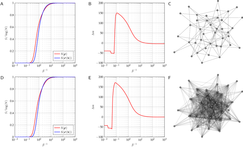
Figure 1: Normalized von Neumann entropy and reconstruction error of a random network (top panels) and its ensemble average with the same degree sequence (bottom panels). In panels A,D the red curves are the spectral entropy of the observed network described by density $\boldsymbol{\rho}$, blue curves are the spectral entropies of the model network at optimum parameters $\boldsymbol{\sigma}(\tilde{\boldsymbol{\theta}})$. In panel B a systematic error exists at every $\beta$ (even in the limit $\beta\to 0$): in the spectral framework the UBCM cannot fit all the specific properties of the highly ordered network. On the other hand, an ensemble average network has a structure that can be better reconstructed by the UBCM, as shown by the error $\Delta m$ going to zero in Panel E.

As a second example we chose a toy network consisting of a number of cliques of increasing size connected in a ring, and one of its degree-preserving random rewiring ( Figure 2C,F). In the ordered case, the clique structure cannot be accounted by a first-order average model alone, making that specific instance highly unlikely in our framework when sampling from the configuration model. Therefore, following the fitting procedure described above, one can see a significant difference in the number of links between model and data $\Delta m$ even at a very small beta Figure 2B. In other words, in the ordered case, the degree sequence alone cannot explain the differences in the spectral entropies, thus indicating the presence of genuine regular patterns that substantially alter the properties of diffusion of the random walker defined by the density matrix. Indeed, this difference reflects the intrinsic inability of the model to account for the characteristic structure of the underlying network.

After fitting, non vanishing $\Delta m$ serves as an indicator of the presence of ordered patterns in the given network that are not explained by this model alone. To test this idea we applied the same optimization technique to the degree-preserving randomly rewired network in Figure 2F, and plotted the results in Figure 2D,E. In this case the random rewiring made the empirical network more adherent to the optimal reconstruction by the model and the difference in the total number of links at $\beta$ close to zero is much smaller than in the ordered case. This is also evident by the better adherence in the spectral entropies, as shown in Figure 2D.

Importantly, the spectral entropy optimization framework described above can be applied to descriptive network models other than those described by the exponential random graph model.

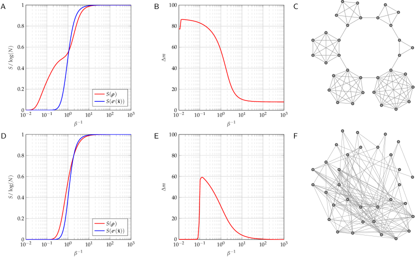
Figure 2: Normalized von Neumann entropy and reconstruction error of two networks: a ring of cliques (top panels) and its degree-preserving random rewiring (bottom panels). In panels A,D the red curves are the spectral entropy of the observed network described by density $\boldsymbol{\rho}$, blue curves are the spectral entropies of the model network at optimum parameters $\boldsymbol{\sigma}(\tilde{\boldsymbol{\theta}})$. In panel B a systematic error exists at every $\beta$ (even in the limit $\beta\to 0$): the UBCM cannot fit all the specific properties of the highly ordered network. On the other hand, a degree preserving rewired network has a structure that can be better reconstructed by the UBCM, as shown by the error $\Delta m$ going to zero in Panel E.

V Spatial models

The embedding of a network in a two or three dimensional space has bearings on its topological properties. When the formation of links has a cost associated with distance, the model must accomodate additional spatial constraints, which introduce correlation between topological and geometrical organization Barthélemy (2011). An example is represented by neural networks, in which communication between neurons implies a metabolic cost that depends on their distance Bullmore and Sporns (2012); Betzel and Bassett (2017). The material and metabolic constraints of neuronal wiring are factors that contributed to shaping brain architecture Bullmore and Sporns (2012); Stam and van Straaten (2012); Ribrault et al. (2011). Computational and empirical studies converged on the result that a multiscale organization of modules inside modules is the one that satisfies the constraints imposed by minimization of energetic cost and spatial embedding Bullmore and Sporns (2012); Doucet et al. (2011); Betzel and Bassett (2017); Kaiser and Hilgetag (2006). Here, wiring cost includes the physical volume of axons and synapses, the energetic demand for signal transmission, additional processing cost for noise correction over long distance signaling and sustenance of the necessary neuroglia that support neuronal activities Bullmore and Sporns (2012). Therefore, it is tempting to assume that the expected number of neural fibers between two areas could be expressed as a decreasing function of their length. With this hypothesis in mind, we verified the ability of our optimization approach to work with a simple descriptive model of the observed neural connectivity in the macaque cortex Markov et al. (2014); Ercsey-Ravasz et al. (2013). The model, called Exponential Distance Rule (EDR), is a dense weighted network model describing the decline in the expected number of axonal projections $w_{ij}$ as a function of the inter-areal distances $d_{ij}$ and a tunable decay parameter $\ell\in\mathbb{R}$:

$${\mathbb{E}}[w_{ij}]=Ce^{-\ell d_{ij}},$$ (24)

where $C$ is a normalization constant. Here, the distances $d_{ij}$ are measured along the shortest path connecting areas via white matter, approximating the axonal distance Markov et al. (2014).

We used a dataset of cortico-cortical connectivity generated from retrograde tracing experiments in the macaque brain Ercsey-Ravasz et al. (2013); Markov et al. (2014). Following the procedure introduced in the previous sections, we fitted the macaque connectome network with the EDR model. Differently from the random graph models described in previous sections, we found an optimal inverse-temperature parameter $\beta$ that minimizes the reconstruction error, as shown in Figure 3B. At this optimal $\beta^{*}\approx 3.05$ the reconstructed decay parameter $\tilde{\ell}=0.1505$ $[\textrm{mm}]^{-1}$ is comparable to the values obtained by the three methods applied in the original paper from Ref Ercsey-Ravasz et al. (2013). The non-vanishing difference in total weights between reconstructed and object networks indicates that the model cannot account completely for the structures such as the high density core observed in the connectome Ercsey-Ravasz et al. (2013). Hence, a non-zero optimal value for $\beta$ suggests the existence of a scale at which the model best describes the topological properties of the network.

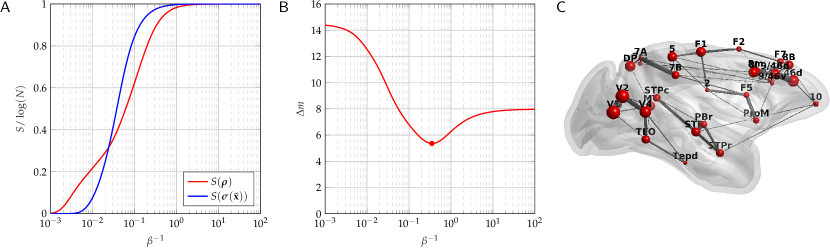
Figure 3: Normalized von Neumann entropy and reconstruction error of the macaque brain connectivity network (panel C). In panel A the red curve is the spectral entropy of the observed network described by density $\boldsymbol{\rho}$, blue curve is the spectral entropy of the model network at optimum parameter $\boldsymbol{\sigma}(\tilde{\boldsymbol{\theta}})$. The optimal hyperparameter $\beta$ is found in panel B where the reconstruction error $\Delta m$ achieve its minimum denoted by a red dot.

VI Conclusion

The spectral entropies framework enables comparing networks taking into account the whole structure at multiple scales. However, this approach introduces a hyperparameter $\beta$ that plays the role of an inverse temperature, and whose tuning is critical for the correct estimate of the model parameters.

Leveraging a thermodynamic analogy, we have shown that the optimal value of the hyperparameter is model dependent and reflects the scales at which the model best describes the empirical network. Moreover, we have described procedures to determine $\beta$ for the model parameter optimization and for a tractable approximation of the expected relative entropy.

Specifically, we focused on three examples from the exponential random graph model, namely the Erdős-Rényi, a planted partition and undirected binary configuration model. In the Erdős-Rényi model and in the planted partition model, we analytically demonstrated that correct reconstruction is possible only in the infinite temperature limit. In the configuration model this hypothesis was verified numerically. The presence of ordered structures unaccounted for by the model is reflected in a bias of the total energy, corresponding to the total number of links in the reconstructed network.

Motivated by these findings in synthetic networks, we applied the spectral entropy framework to a real-world network of the macaque brain structural connectome. A structural connectome is a spatial network whose development is thought to be constrained by geometrical and wiring cost factors. Hence, we evaluated an exponential distance rule model that assumes that the weight of inter-areal connections is a decreasing function of distance. We demonstrate the existence of a non-zero optimal value of $\beta$ for the computation of model parameters. However, the residual energy bias indicates the network structure at certain scales cannot be described by the exponential distance rule model alone.

The procedures demonstrated here make it possible to use relative entropy methods for practical applications to the study of models of real-world networks, effectively realizing a conceptual step from classical maximum likelihood methods to their density matrix based counterparts.

Appendix A Approximation of expected relative entropy

We can exploit the commutativity and linearity of the trace and expectation operators to obtain a simpler expression for the expected relative entropy:

$$\mathbb{E}_{\boldsymbol{\theta}}[S(\boldsymbol{\rho}\|\boldsymbol{\sigma}(\boldsymbol{\theta})]=\operatorname{Tr}\left[\boldsymbol{\rho}\log\boldsymbol{\rho}\right]-\operatorname{Tr}\left[\boldsymbol{\rho}\mathbb{E}_{\boldsymbol{\theta}}\left[\log\boldsymbol{\sigma}(\boldsymbol{\theta})\right]\right].$$ (25)

By the positive-definiteness of the density $\boldsymbol{\sigma}$, we have:

$$\log(\boldsymbol{\sigma}(\boldsymbol{\theta}))=-\beta\mathbf{L}(\boldsymbol{\theta})-\mathbf{I}\log Z(\boldsymbol{\theta}).$$ (26)

Plugging this into the expression of the expected relative entropy we obtain:

$$\mathbb{E}_{\boldsymbol{\theta}}[S(\boldsymbol{\rho}\|\boldsymbol{\sigma}(\boldsymbol{\theta})]=\operatorname{Tr}\left[\boldsymbol{\rho}\left(\log\boldsymbol{\rho}+\beta\mathbb{E}_{\boldsymbol{\theta}}[\mathbf{L}(\boldsymbol{\theta})]+\mathbf{I}\mathbb{E}_{\boldsymbol{\theta}}\left[\log Z(\boldsymbol{\theta})\right]\right)\right]$$ (27)

This last expression depends on the expected Laplacian of the model $\mathbb{E}_{\boldsymbol{\theta}}[\mathbf{L}(\boldsymbol{\theta})]$ and on the expected log-partition function $\mathbb{E}_{\boldsymbol{\theta}}[\log Z(\boldsymbol{\theta})]$. An analytical estimate of the expected Laplacian as function of the parameters $\boldsymbol{\theta}$ can readily be obtained, but computation of the expected log-partition function $\mathbb{E}_{\boldsymbol{\theta}}[\log Z(\boldsymbol{\theta})]$ is more difficult and requires techniques from random matrix theory Nadakuditi and Newman (2012); Peixoto (2013); Nadakuditi and Newman (2013). This is clear as the trace of a matrix is equal to the sum of its eigenvalues, yielding:

$$\mathbb{E}_{\boldsymbol{\theta}}\left[\log Z(\boldsymbol{\theta})\right]=\mathbb{E}_{\boldsymbol{\theta}}\left[\log\left(\sum_{i=1}^{n}e^{-\beta\lambda_{i}(\mathbf{L}(\boldsymbol{\theta}))}\right)\right].$$ (28)

We can estimate the expected log-partition function by means of matrix concentration arguments Tropp (2015); Cape et al. (2017). A random matrix is said to concentrate when, given some spectral norm, one can tightly bound the spectral norm of the difference from its expected value Qiu and Wicks (2014). In the case of network-related matrices, the eigenvalues of the Laplacian and those of its expectation are strictly related and can be tightly bounded with high probability Oliveira (2009); Preciado and Rahimian (2017); Cape et al. (2017). This approximation becomes more precise, the larger and denser the graphs are Le et al. (2015, 2017), an effect of the concentration of measure phenomenon. Therefore, following the ideas presented in references Cape et al. (2017); Oliveira (2009) that apply in our same settings, we replace $\lambda_{i}(\mathbf{L}(\boldsymbol{\theta}))$ with their counterparts from the expected Laplacian $\lambda_{i}(\mathbb{E}_{\boldsymbol{\theta}}[\mathbf{L}])$. Substituting back, we recover an expression that involves the relative entropy between the observed density and the density of the expected Laplacian:

$$\mathbb{E}_{\boldsymbol{\theta}}[S(\boldsymbol{\rho}\|\boldsymbol{\sigma}(\boldsymbol{\theta}))]\approx S(\boldsymbol{\rho}\|\boldsymbol{\sigma}(\mathbb{E}_{\boldsymbol{\theta}}[\mathbf{L}])).$$ (29)

Appendix B Gradients of the relative entropy

Here we present the analytical calculation of the gradients of the relative entropy described in Eq. 10. We can decompose the relative entropy using Eq. 26 as:

$$S(\boldsymbol{\rho}\|\boldsymbol{\sigma}(\mathbb{E}_{\boldsymbol{\theta}}[\mathbf{L}]))=\beta\operatorname{Tr}\left[\boldsymbol{\rho}\mathbb{E}_{\boldsymbol{\theta}}[\mathbf{L}(\boldsymbol{\theta})]\right]+\log\operatorname{Tr}\left[e^{-\beta\mathbb{E}_{\boldsymbol{\theta}}[\mathbf{L}(\boldsymbol{\theta})]}\right]$$ (30)

where we have used the fact that $\operatorname{Tr}\left[\boldsymbol{\rho}\mathbf{I}\right]=\operatorname{Tr}\left[\boldsymbol{\rho}\right]=1$ by definition of density matrix. Taking the derivatives with respect to the $k$-th parameter $\theta_{k}$, and by linearity of the trace operator, we get:

$$\frac{\partial S(\boldsymbol{\rho}\|\boldsymbol{\sigma}(\mathbb{E}_{\boldsymbol{\theta}}[\mathbf{L}(\boldsymbol{\theta})]))}{\partial\theta_{k}}= \beta\operatorname{Tr}\left[\boldsymbol{\rho}\frac{\partial\mathbb{E}_{\boldsymbol{\theta}}[\mathbf{L}(\boldsymbol{\theta})]}{\partial\theta_{k}}\right]$$

$$+\frac{\partial}{\partial\theta_{k}}\log\operatorname{Tr}\left[e^{-\beta\mathbb{E}_{\boldsymbol{\theta}}[\mathbf{L}(\boldsymbol{\theta})]}\right]$$ (31)

The following identity holds for the derivatives of the matrix exponential function:

$$\frac{d}{dt}\operatorname{Tr}\left[e^{\mathbf{X}(t)}\right]=\operatorname{Tr}\left[e^{\mathbf{X}(t)}\frac{d\mathbf{X}(t)}{dt}\right],$$ (32)

so we can simply compute the second term involving the log-trace by standard calculus tools. After some algebraic manipulation, we finally arrive to the expression for the derivative of the relative entropy with respect to the model parameters as described in the main text:

$$\frac{\partial S(\boldsymbol{\rho}\|\boldsymbol{\sigma}(\mathbb{E}[\mathbf{L}]))}{\partial\theta_{k}}=\beta\operatorname{Tr}\left[\left(\boldsymbol{\rho}-\boldsymbol{\sigma}(\mathbb{E}_{\boldsymbol{\theta}}[\mathbf{L}(\boldsymbol{\theta})])\right)\frac{\partial\mathbb{E}_{\boldsymbol{\theta}}[\mathbf{L}(\boldsymbol{\theta})]}{\partial\theta_{k}}\right]$$ (33)

References

- Newman (2010) Mark Newman. Networks: An Introduction. OUP Oxford, 2010.
- Barabasi and Albert (1999) Albert-Laszlo Barabasi and Reka Albert. Emergence of scaling in random networks. Science, 286(5439):509–512, 1999.
- Caldarelli (2007) Guido Caldarelli. Scale-free networks: complex webs in nature and technology. Oxford University Press, 2007.
- Bullmore and Sporns (2009) Ed Bullmore and Olaf Sporns. Complex brain networks: graph theoretical analysis of structural and functional systems. Nat. Rev. Neurosci., 10(3):186–198, 2009. ISSN 1471-0048.
- Wasserman and Faust (1994) Stanley Wasserman and Katherine Faust. Social network analysis: Methods and applications, volume 8. Cambridge university press, 1994.
- Squartini and Garlaschelli (2017) Tiziano Squartini and Diego Garlaschelli. Maximum-Entropy Networks: Pattern Detection, Network Reconstruction and Graph Combinatorics. Springer, 2017.
- De Domenico and Biamonte (2016) Manlio De Domenico and Jacob Biamonte. Spectral entropies as information-theoretic tools for complex network comparison. Phys. Rev. X, 041062:1–13, 2016.
- Parrondo et al. (2015) Juan M.R. Parrondo, Jordan M. Horowitz, and Takahiro Sagawa. Thermodynamics of information. Nat. Phys., 11(2):131–139, 2015.
- Park and Newman (2004) Juyong Park and M. E. J. Newman. Statistical mechanics of networks. Phys. Rev. E, 70(6):066117, 2004.
- Jaynes (1957) E. T. Jaynes. Information theory and statistical mechanics. Phys. Rev., 106(4):620–630, 1957.
- Erdös and Rényi (1959) P Erdös and a Rényi. On random graphs. Publ. Math., 6:290–297, 1959. ISSN 00029947.
- Caldarelli et al. (2002) G. Caldarelli, A. Capocci, P. De Los Rios, and M. A. Muñoz. Scale-free networks from varying vertex intrinsic fitness. Phys. Rev. Lett., 89:258702, 2002.
- Squartini et al. (2015) Tiziano Squartini, Rossana Mastrandrea, and Diego Garlaschelli. Unbiased sampling of network ensembles. New J. Phys., 17(2):023052, 2015. ISSN 1367-2630.
- Squartini and Garlaschelli (2014) Tiziano Squartini and Diego Garlaschelli. Jan Tinbergen’s legacy for economic networks: from the gravity model to quantum statistics. Econophysics of Agent-Based Models, pages 161–186, 2014.
- Garlaschelli and Loffredo (2008) Diego Garlaschelli and Maria I. Loffredo. Maximum likelihood: Extracting unbiased information from complex networks. Phys. Rev. E, 78(1):1–4, 2008.
- Braunstein et al. (2006) Samuel L. Braunstein, Sibasish Ghosh, and Simone Severini. The Laplacian of a graph as a density Matrix: A basic combinatorial approach to separability of mixed states. Ann. Comb., 10(3):291–317, 2006.
- Estrada (2011) Ernesto Estrada. The Structure of Complex Networks: Theory and Applications. Oxford University Press, Inc., New York, NY, USA, 2011.
- Anderson (1985) William N Anderson. Eigenvalues of the Laplacian of a graph. Linear Multilinear A., 18(2):141–145, 1985.
- Merris (1994) Russell Merris. Laplacian matrices of graphs: a survey. Linear Algebra Appl., 197-198(C):143–176, 1994.
- de Lange et al. (2014) Siemon C. de Lange, Marcel A. de Reus, and Martijn P. van den Heuvel. The Laplacian spectrum of neural networks. Frontiers in Computational Neuroscience, 7(January):1–12, 2014. ISSN 1662-5188.
- de Lange et al. (2016) Siemon C. de Lange, Martijn P. van den Heuvel, and Marcel A. de Reus. The role of symmetry in neural networks and their Laplacian spectra. NeuroImage, 141:357–365, 2016. ISSN 10959572.
- Cheeger (1970) Jeff Cheeger. A lower bound for the smallest eigenvalue of the laplacian. Problems in analysis, pages 195–199, 1970.
- Donetti et al. (2006) Luca Donetti, Franco Neri, and Miguel A Muñoz. Optimal network topologies: expanders, cages, Ramanujan graphs, entangled networks and all that. J. Stat. Mech-Theory E, 2006(08):P08007, 2006.
- Lovász (1993) L Lovász. Random walks on graphs: A survey. Bolyai Math. Stud., 2(Volume 2):1–46, 1993.
- Masuda et al. (2017) Naoki Masuda, Mason A. Porter, and Renaud Lambiotte. Random walks and diffusion on networks. Phys. Rep., 2017.
- Bray and Rodgers (1988) A. J. Bray and G. J. Rodgers. Diffusion in a sparsely connected space: A model for glassy relaxation. Phys. Rev. B, 38(16):11461–11470, 1988.
- Mohar et al. (1991) Bojan Mohar, Y Alavi, G Chartrand, and OR Oellermann. The laplacian spectrum of graphs. Graph theory, combinatorics, and applications, 2(871-898):12, 1991.
- Anand et al. (2011) Kartik Anand, Ginestra Bianconi, and Simone Severini. Shannon and von Neumann entropy of random networks with heterogeneous expected degree. Phys. Rev. E, 83(3):1–8, 2011.
- Wilde (2013) Mark M Wilde. Quantum information theory. Cambridge University Press, 2013.
- Higham (2008) Nicholas J Higham. Functions of matrices: theory and computation. SIAM, 2008.
- Jaynes (2003) E. T. Jaynes. Probability Theory: The Logic of Science. The Mathematical Intelligencer, 27(2):83–83, 2003. ISSN 0343-6993.
- Biamonte et al. (2017) Jacob Biamonte, Mauro Faccin, and Manlio De Domenico. Complex Networks: from Classical to Quantum. arXiv preprint arXiv:1702.08459, 2017.
- Estrada and Hatano (2008) Ernesto Estrada and Naomichi Hatano. Communicability in complex networks. Phys. Rev. E, 77(3):1–12, 2008.
- Faccin et al. (2013) Mauro Faccin, Tomi Johnson, Jacob Biamonte, Sabre Kais, and Piotr Migdał. Degree Distribution in Quantum Walks on Complex Networks. Phys. Rev. X, 3(4):041007, 2013.
- Estrada et al. (2012) Ernesto Estrada, Naomichi Hatano, and Michele Benzi. The physics of communicability in complex networks. Phys. Rep., 514(3):89–119, 2012.
- Cover and Thomas (2006) Thomas M. Cover and Joy A. Thomas. Elements of Information Theory. Wiley-Interscience, 2006.
- Nadakuditi and Newman (2012) Raj Rao Nadakuditi and Mark EJ Newman. Graph spectra and the detectability of community structure in networks. Phys. Rev. Lett., 108(18):188701, 2012.
- Peixoto (2013) Tiago P. Peixoto. Eigenvalue spectra of modular networks. Phys. Rev. Lett., 111:098701, Aug 2013.
- Nadakuditi and Newman (2013) Raj Rao Nadakuditi and Mark EJ Newman. Spectra of random graphs with arbitrary expected degrees. Phys. Rev. E, 87(1):012803, 2013.
- Robbins and Monro (1951) Herbert Robbins and Sutton Monro. A stochastic approximation method. The annals of mathematical statistics, pages 400–407, 1951.
- Kiefer and Wolfowitz (1952) Jack Kiefer and Jacob Wolfowitz. Stochastic estimation of the maximum of a regression function. The Annals of Mathematical Statistics, pages 462–466, 1952.
- Merhav (2010) Neri Merhav. Statistical Physics and Information Theory. Foundations and Trends in Communications and Information Theory, 6(1-2):1–212, 2010.
- Deffner and Lutz (2010) Sebastian Deffner and Eric Lutz. Generalized clausius inequality for nonequilibrium quantum processes. Phys. Rev. Lett., 105(17):1–4, 2010.
- Condon and Karp (2000) Anne Condon and Richard M Karp. on the Planted Partition Model. Electr. Eng., pages 116–140, 2000.
- Barthélemy (2011) Marc Barthélemy. Spatial networks. Phys. Rep., 499(1-3):1–101, 2011.
- Bullmore and Sporns (2012) Ed Bullmore and Olaf Sporns. The economy of brain network organization. Nat. Rev. Neurosci., 13(5):336–349, 2012. ISSN 1471-0048.
- Betzel and Bassett (2017) Richard F Betzel and Danielle S Bassett. Generative models for network neuroscience: prospects and promise. J. R. Soc. Interface, 14(136):20170623, 2017.
- Stam and van Straaten (2012) C. J. Stam and E. C W van Straaten. The organization of physiological brain networks. Clin. Neurophysiol., 123(6):1067–1087, 2012. ISSN 13882457.
- Ribrault et al. (2011) Claire Ribrault, Ken Sekimoto, and Antoine Triller. From the stochasticity of molecular processes to the variability of synaptic transmission. Nat. Rev. Neurosci., 12(7):375–387, 2011.
- Doucet et al. (2011) Gaëlle Doucet, Mikaël Naveau, Laurent Petit, Nicolas Delcroix, Laure Zago, Fabrice Crivello, Gaël Jobard, Nathalie Tzourio-Mazoyer, Bernard Mazoyer, Emmanuel Mellet, and Marc Joliot. Brain activity at rest: a multiscale hierarchical functional organization. J. Neurophysiol., 105(6):2753–2763, 2011. ISSN 1522-1598.
- Kaiser and Hilgetag (2006) Marcus Kaiser and Claus C Hilgetag. Nonoptimal component placement, but short processing paths, due to long-distance projections in neural systems. PLoS Comput. Biol., 2(7):e95, 2006.
- Markov et al. (2014) N. T. Markov et al. A weighted and directed interareal connectivity matrix for macaque cerebral cortex. Cereb. Cortex, 24(1):17–36, 2014.
- Ercsey-Ravasz et al. (2013) Mária Ercsey-Ravasz, Nikola T. Markov, Camille Lamy, David C. VanEssen, Kenneth Knoblauch, Zoltán Toroczkai, and Henry Kennedy. A Predictive Network Model of Cerebral Cortical Connectivity Based on a Distance Rule. Neuron, 80(1):184–197, 2013.
- Tropp (2015) Joel A. Tropp. An introduction to matrix concentration inequalities. Found. Trends Mach. Learn., 8(1-2):1–230, 2015. ISSN 1935-8237.
- Cape et al. (2017) Joshua Cape, Minh Tang, and Carey E. Priebe. The kato-temple inequality and eigenvalue concentration with applications to graph inference. Electron. J. Stat., 11(2):3954–3978, 2017. ISSN 19357524.
- Qiu and Wicks (2014) Robert Qiu and Michael Wicks. Cognitive networked sensing and big data, volume 9781461445449. 2014. ISBN 9781461445449.
- Oliveira (2009) Roberto Imbuzeiro Oliveira. Concentration of the adjacency matrix and of the Laplacian in random graphs with independent edges. arXiv:0911.0600, pages 1–46, nov 2009.
- Preciado and Rahimian (2017) Victor M Preciado and M Amin Rahimian. Moment-based spectral analysis of random graphs with given expected degrees. IEEE Transactions on Network Science and Engineering, 4(4):215–228, 2017.
- Le et al. (2015) Cm Le, E Levina, and R Vershynin. Sparse random graphs: regularization and concentration of the Laplacian. arXiv:1502.03049, page 31, 2015.
- Le et al. (2017) Can M. Le, Elizaveta Levina, and Roman Vershynin. Concentration and regularization of random graphs. Random Struct. & Algor., 51(3):538–561, 2017. ISSN 10982418.