Code Constructions for Distributed Storage With Low Repair Bandwidth and Low Repair Complexity

Abstract

We present the construction of a family of erasure correcting codes for distributed storage that achieve low repair bandwidth and complexity at the expense of a lower fault tolerance. The construction is based on two classes of codes, where the primary goal of the first class of codes is to provide fault tolerance, while the second class aims at reducing the repair bandwidth and repair complexity. The repair procedure is a two-step procedure where parts of the failed node are repaired in the first step using the first code. The downloaded symbols during the first step are cached in the memory and used to repair the remaining erased data symbols at minimal additional read cost during the second step. The first class of codes is based on MDS codes modified using piggybacks, while the second class is designed to reduce the number of additional symbols that need to be downloaded to repair the remaining erased symbols. We numerically show that the proposed codes achieve better repair bandwidth compared to MDS codes, codes constructed using piggybacks, and local reconstruction/Pyramid codes, while a better repair complexity is achieved when compared to MDS, Zigzag, Pyramid codes, and codes constructed using piggybacks.

I Introduction

In recent years, there has been a widespread adoption of distributed storage systems (DSSs) as a viable storage technology for Big Data. Distributed storage provides an inexpensive storage solution for storing large amounts of data. Formally, a DSS is a network of numerous inexpensive disks (or nodes) where data is stored in a distributed fashion. Storage nodes are prone to failures, and thus to losing the stored data. Reliability against node failures (commonly referred to as fault tolerance) is achieved by means of erasure correcting codes (ECCs). ECCs are a way of introducing structured redundancy, and for a DSS, it means addition of redundant nodes. In case of a node failure, these redundant nodes allow complete recovery of the data stored. Since ECCs have a limited fault tolerance, to maintain the initial state of reliability, when a node fails a new node needs to be added to the DSS network and populated with data. The problem of repairing a failed node is known as the repair problem.

Current DSSs like Google File System ii@ and Quick File System use a family of Reed-Solomon (RS) ECCs [1]. Such codes come under a broader family of maximum distance separable (MDS) codes. MDS codes are optimal in terms of the fault tolerance/storage overhead tradeoff. However, the repair of a failed node requires the retrieval of large amounts of data from a large subset of nodes. Therefore, in the recent years, the design of ECCs that reduce the cost of repair has attracted significant attention. Pyramid codes [2] were one of the first code constructions that addressed this problem. In particular, Pyramid codes are a class of non-MDS codes that aim at reducing the number of nodes that need to be contacted to repair a single failed node, known as the repair locality. Other non-MDS codes that reduce the repair locality are local reconstruction codes (LRCs) [3] and locally repairable codes [4, 5]. Such codes achieve a low repair locality by ensuring that the parity symbols are a function of a small number of data symbols, which also entails a low repair complexity, defined as the number of elementary additions required to repair a failed node. Furthermore, for a fixed locality LRCs and Pyramid codes achieve the optimal fault tolerance.

Another important parameter related to the repair is the repair bandwidth, defined as the number of symbols downloaded to repair a single failed node. Dimakis et al. [6] derived an optimal repair bandwidth-storage per node tradeoff curve and defined two new classes of codes for DSSs known as minimum storage regenerating (MSR) codes and minimum bandwidth regenerating (MBR) codes that are at the two extremal points of the tradeoff curve. MSR codes are MDS codes with the best storage efficiency, i.e., they require a minimum storage of data per node (referred to as the sub-packetization level). On the other hand, MBR codes achieve the minimum repair bandwidth. Product-Matrix MBR (PM-MBR) codes and Fractional Repetition (FR) codes in [7] and [8], respectively, are examples of MBR codes. In particular, FR codes achieve low repair complexity at the cost of high storage overheads. Codes such as minimum disk input/output repairable (MDR) codes [9] and Zigzag codes [10] strictly fall under the class of MSR codes. These codes have a high sub-packetization level. Alternatively, the MSR codes presented in [11, 12, 13, 14, 15, 16, 17, 18] achieve the minimum possible sub-packetization level.

Piggyback codes presented in [19] are another class of codes that achieve a sub-optimal reduction in repair bandwidth with a much lower sub-packetization level in comparison to MSR codes, using the concept of piggybacking. Piggybacking consists of adding carefully chosen linear combinations of data symbols (called piggybacks) to the parity symbols of a given ECC. This results in a lower repair bandwidth at the expense of a higher complexity in encoding and repair operations. More recently, the authors in [20] presented a family of codes that reduce the encoding and repair complexity of PM-MBR codes while maintaining the same level of fault tolerance and repair bandwidth. However, this comes at the cost of large alphabet size. In [21], binary MDS array codes that achieve optimal repair bandwidth and low repair complexity were introduced, with the caveat that the file size is asymptotic and that the fault tolerance is limited to $3$.

In this paper, we propose a family of non-MDS ECCs that achieve low repair bandwidth and low repair complexity while keeping the field size relatively small and having variable fault tolerance. In particular, we propose a systematic code construction based on two classes of parity symbols. Correspondingly, there are two classes of parity nodes. The first class of parity nodes, whose primary goal is to provide erasure correcting capability, is constructed using an MDS code modified by applying specially designed piggybacks to some of its code symbols. As a secondary goal, the first class of parity nodes enable to repair a number of data symbols at a low repair cost by downloading piggybacked symbols. The second class of parity nodes is constructed using a block code whose parity symbols are obtained through simple additions. The purpose of this class of parity nodes is not to enhance the erasure correcting capability, but rather to facilitate node repair at low repair bandwidth and low repair complexity by repairing the remaining failed symbols in the node. Compared to [22], we provide two constructions for the second class of parity nodes. The first one is given by a simple equation that represents the algorithmic construction in [22]. The second one is a heuristic construction that is more involved, but further reduces the repair bandwidth in some cases. Furthermore, we provide explicit formulas for the fault tolerance, repair bandwidth, and repair complexity of the proposed codes and numerically compare with other codes in the literature. The proposed codes achieve better repair bandwidth compared to MDS codes, Piggyback codes, generalized Piggyback codes [23], and exact-repairable MDS codes [24]. For certain code parameters, we also see that the proposed codes have better repair bandwidth compared to LRCs and Pyramid codes. Furthermore, they achieve better repair complexity than Zigzag codes, MDS codes, Piggyback codes, generalized Piggyback codes, exact-repairable MDS codes, and binary addition and shift implementable cyclic-convolutional (BASIC) PM-MBR codes [20]. Also, for certain code parameters, the codes have better repair complexity than Pyramid codes. The improvements over MDS codes, MSR codes, and the classes of Piggyback codes come at the expense of a lower fault tolerance in general.

II System Model and Code Construction

We consider the DSS depicted in Fig. 1, consisting of storage nodes, of which $k$ are data nodes and $n-k$ are parity nodes. Consider a file that needs to be stored on the DSS. We represent a file as a $k\times k$ matrix $\bm{D}=[d_{i,j}]$, called the data array, over $\text{GF}(q)$, where $\text{GF}(q)$ denotes the Galois field of size $q$, with $q$ being a prime number or a power of a prime number. In order to achieve reliability against node failures, the matrix $\bm{D}$ is encoded using an $(n,k)$ vector code [25] to obtain a code matrix $\bm{C}=[c_{i,j}]$, referred to as the code array, of size $k\times n$, $c_{i,j}\in\text{GF}(q)$. The symbol $c_{i,j}$ in $\bm{C}$ is then stored at the $i$-th row of the $j$-th node in the DSS. Thus, each node stores $k$ symbols. Each row in $\bm{C}$ is referred to as a stripe so that each file in the DSS is stored over $k$ stripes in $n$ storage nodes. We consider the $(n,k)$ code to be systematic, which means that $c_{i,j}=d_{i,j}$ for $i,j=0,\ldots,k-1$. Correspondingly, we refer to the $k$ nodes storing systematic symbols as data nodes and the remaining $n-k$ nodes containing parity symbols only as parity nodes. The efficiency of the code is determined by the code rate, given by $R=k^{2}/kn=k/n$. Alternatively, the inverse of the code rate is referred to as the storage overhead.

For later use, we denote the set of message symbols in the $k$ data nodes as $\mathcal{D}=\{d_{i,j}\}$ and by $\mathcal{P}_{t}$, $t=k,\ldots,n-1$, the set of parity symbols in the $t$-th node. Subsequently, we define the set $\mathcal{D}_{\mathcal{I}}\subseteq\mathcal{D}$ as

$$\mathcal{D}_{\mathcal{I}}=\{d_{i,j}\in\mathcal{D}\mid(i,j)\in\mathcal{I}\},$$

where $\mathcal{I}$ is an arbitrary index set. We also define the operator $(a+b)_{k}\triangleq(a+b)\bmod k$ for integers $a$ and $b$.

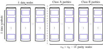
Figure 1: System model of the DSS.

Our main goal is to construct codes that yield low repair bandwidth and low repair complexity of a single failed data node. We focus on the repair of data nodes since the raw data is stored on these nodes and the users can readily access the data through these nodes. Thus, their survival is a crucial aspect of a DSS. To this purpose, we construct a family of systematic $(n,k)$ codes consisting of two different classes of parity symbols. Correspondingly, there are two classes of parity nodes, referred to as Class ${\mathsf{A}}$ and Class ${\mathsf{B}}$ parity nodes, as shown in Fig. 1. Class ${\mathsf{A}}$ and Class ${\mathsf{B}}$ parity nodes are built using an $(n_{\mathsf{A}},k)$ code and an $(n_{\mathsf{B}},k)$ code, respectively, such that $n=n_{\mathsf{A}}+n_{\mathsf{B}}-k$. In other words, the parity nodes from the $(n,k)$ code correspond to the parity nodes of Class ${\mathsf{A}}$ and Class ${\mathsf{B}}$ codes. The primary goal of Class ${\mathsf{A}}$ parity nodes is to achieve a good erasure correcting capability, while the purpose of Class ${\mathsf{B}}$ nodes is to yield low repair bandwidth and low repair complexity. In particular, we focus on the repair of data nodes. The repair bandwidth (in bits) per node, denoted by $\gamma$, is proportional to the average number of symbols (data and parity) that need to be downloaded to repair a data symbol, denoted by $\lambda$. More precisely, let $\beta$ be the sub-packetization level of the DSS, which is the number of symbols per node. Then,

$$\lambda=\frac{\gamma}{\nu\beta},$$ (1)

where $\nu=m\lceil\log_{2}p\rceil$ is the size (in bits) of a symbol in $\text{GF}(q)$, where $q=p^{m}$ for some prime number $p$ and positive integer $m$. $\lambda$ can be interpreted as the repair bandwidth normalized by the size (in bits) of a node, and will be referred to as the normalized repair bandwidth.

The main principle behind our code construction is the following. The repair is performed one symbol at a time. After the repair of a data symbol is accomplished, the symbols read to repair that symbol are cached in the memory. Therefore, they can be used to repair the remaining data symbols at no additional read cost. The proposed codes are constructed in such a way that the repair of a new data symbol requires a low additional read cost (defined as the number of additional symbols that need to be read to repair the data symbol), so that $\lambda$ (and hence $\gamma$) is kept low.

Definition 1

The read cost of a symbol is the number of symbols that need to be read to repair the symbol. For a symbol that is repaired after some others, the additional read cost is defined as the number of additional symbols that need to be read to repair the symbol. (Note that symbols previously read to repair other data symbols are already cached in the memory and to repair a new symbol only some extra symbols may need to be read.)

III Class ${\mathsf{A}}$ Parity Nodes

Class ${\mathsf{A}}$ parity nodes are constructed using a modified $(n_{\mathsf{A}},k)$ MDS code, with $k+2\leq n_{\mathsf{A}}<2k$, over $\text{GF}(q)$. In particular, we start from an $(n_{\mathsf{A}},k)$ MDS code and apply piggybacks [19] to some of the parity symbols. The construction of Class ${\mathsf{A}}$ parity nodes is performed in two steps as follows.

1. Encode each row of the data array using an $(n_{\mathsf{A}},k)$ MDS code (same code for each row). The parity symbol $p^{{\mathsf{A}}}_{i,j}$ is obtained as

   $$p^{{\mathsf{A}}}_{i,j}=\sum_{l=0}^{k-1}\alpha_{l,j}d_{i,l},~{}j=k,\ldots,n_{\mathsf{A}}-1,$$ (2)

   where $\alpha_{l,j}$ denotes a coefficient in $\text{GF}(q)$ and $i=0,\ldots,k-1$. Store the parity symbol in the corresponding row of the code array. Overall, $k(n_{\mathsf{A}}-k)$ parity symbols are generated.

2. Modify some of the parity symbols by adding piggybacks. Let $\tau$, $1\leq\tau\leq n_{\mathsf{A}}-k-1$, be the number of piggybacks introduced per row. The parity symbol $p_{i,u}^{{\mathsf{A}}}$ is updated as

   $$p^{{\mathsf{A}},\mathsf{p}}_{i,u}=p^{{\mathsf{A}}}_{i,u}+d_{(i+u-n_{\mathsf{A}}+\tau+1)_{k},i},$$ (3)

   where $u=n_{\mathsf{A}}-\tau,\ldots,n_{\mathsf{A}}-1$, the second term in the summation is the piggyback, and the superscript $\mathsf{p}$ in $p^{{\mathsf{A}},\mathsf{p}}_{i,u}$ indicates that the parity symbol contains piggybacks.

The fault tolerance (i.e., the number of node failures that can be tolerated) of Class ${\mathsf{A}}$ codes is given in the following theorem.

Theorem 1

An $(n_{\mathsf{A}},k)$ Class ${\mathsf{A}}$ code with $\tau$ piggybacks per row can tolerate

$$f=\begin{cases}n_{\mathsf{A}}-k-\tau+\bigg{\lfloor}\frac{\sqrt{(n_{\mathsf{A}}-k-\tau)^{2}+4k}-(n_{\mathsf{A}}-k-\tau)}{2}\bigg{\rfloor}&\text{if}\,\,\tau\geq\xi\\ n_{\mathsf{A}}-k&\text{if}\,\,\tau<\xi\end{cases}$$

node failures, where $\xi=\frac{\sqrt{(n_{\mathsf{A}}-k-\tau)^{2}+4k}-(n_{\mathsf{A}}-k-\tau)}{2}$.

Proof:

See Appendix A. ∎

We remark that for $\tau<\xi$, Class ${\mathsf{A}}$ codes are MDS codes.

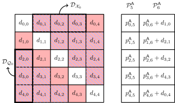
Figure 2: A $(7,5)$ Class ${\mathsf{A}}$ code with $\tau=1$ constructed from a $(7,5)$ MDS code. $\mathcal{P}_{5}^{{\mathsf{A}}}$ and $\mathcal{P}_{6}^{{\mathsf{A}}}$ are the parity nodes. For each row $j$, colored symbols belong to $\mathcal{D}_{\mathcal{R}_{j}}$.

When a failure of a data node occurs, Class ${\mathsf{A}}$ parity nodes are used to repair $\tau+1$ of the $k$ failed symbols. Class ${\mathsf{A}}$ parity symbols are constructed in such a way that, when node $j$ is erased, $\tau+1$ data symbols in this node can be repaired reading the (non-failed) $k-1$ data symbols in the $j$-th row of the data array and $\tau+1$ parity symbols in the $j$-th row of Class ${\mathsf{A}}$ parity nodes (see also Section IV-C). For later use, we define the set $\mathcal{R}_{j}$ as follows.

Definition 2

For $j=0,\ldots,k-1$, the index set $\mathcal{R}_{j}$ is defined as

$$\mathcal{R}_{j}=\{(j,(j+1)_{k}),(j,(j+2)_{k}),\ldots,(j,(j+k-1)_{k})\}.$$

Then, the set $\mathcal{D}_{\mathcal{R}_{j}}$ is the set of $k-1$ data symbols that are read from row $j$ to recover $\tau+1$ data symbols of node $j$ using Class ${\mathsf{A}}$ parity nodes.

Example 1

An example of a Class ${\mathsf{A}}$ code is shown in Fig. 2. One can verify that the code can correct any $2$ node failures. For each row $j$, the set $\mathcal{D}_{\mathcal{R}_{j}}$ is indicated in red color. For instance, $\mathcal{D}_{\mathcal{R}_{0}}=\{d_{0,1},d_{0,2},d_{0,3},d_{0,4}\}$.

The main purpose of Class ${\mathsf{A}}$ parity nodes is to provide good erasure correcting capability. However, the use of piggybacks helps also in reducing the number of symbols that need to be read to repair the $\tau+1$ symbols of a failed node that are repaired using the Class ${\mathsf{A}}$ code, as compared to MDS codes. The remaining $k-\tau-1$ data symbols of the failed node can also be recovered from Class ${\mathsf{A}}$ parity nodes, but at a high symbol read cost of $k$. Hence, the idea is to add another class of parity nodes, namely Class ${\mathsf{B}}$ parity nodes, in such a way that these symbols can be recovered with lower read cost.

IV Class ${\mathsf{B}}$ Parity Nodes

Class ${\mathsf{B}}$ parity nodes are obtained using an $(n_{\mathsf{B}},k)$ linear block code with $n_{\mathsf{B}}<2k-\tau$ over $\text{GF}(q)$ to encode the $k\times k$ data symbols of the data array. This generates $k(n_{\mathsf{B}}-k)$ Class ${\mathsf{B}}$ parity symbols, $p^{{\mathsf{B}}}_{i,l}$, $i=0,\ldots,k-1$, $l=n_{\mathsf{A}},\ldots,n-1$. In [22], we presented an algorithm to construct Class ${\mathsf{B}}$ codes. In this section, we present a similar construction in a much more compact, mathematical manner.

IV-A Definitions and Preliminaries

Definition 3

For $j=0,\ldots,k-1$, the index set $\mathcal{Q}_{j}$ is defined as

$${\mathcal{Q}_{j}}=$$

$$\{((j+\tau+1)_{k},j),((j+\tau+2)_{k},j),\ldots,((j+k-1)_{k},j)\}.$$

Assume that data node $j$ fails. It is easy to see that the set $\mathcal{D}_{\mathcal{Q}_{j}}$ is the set of $k-\tau-1$ data symbols that are not recovered using Class ${\mathsf{A}}$ parity nodes.

Example 2

For the example in Fig. 2, the set $\mathcal{D}_{\mathcal{Q}_{j}}$ is indicated by hatched symbols for each column $j$, $j=0,\ldots,k-1$. For instance, $\mathcal{D}_{\mathcal{Q}_{0}}=\{d_{2,0},d_{3,0},d_{4,0}\}$.

For later use, we also define the following set.

Definition 4

For $j=0,\ldots,k-1$, the index set $\mathcal{X}_{j}$ is defined as

$$\mathcal{X}_{j} =\{(j,(j+1)_{k}),(j,(j+2)_{k}),\ldots,(j,(j+k-\tau-1)_{k})\}.$$

Note that $\mathcal{X}_{j}=\mathcal{R}_{j}\cap\{\cup_{l=0}^{k-1}\mathcal{Q}_{l}\}$.

Example 3

For the example in Fig. 2, the set $\mathcal{D}_{\mathcal{X}_{j}}$ is indicated by hatched symbols for each row $j$. For instance, $\mathcal{X}_{0}=\mathcal{R}_{0}\cap\{\mathcal{Q}_{0}\cup\mathcal{Q}_{1}\cup\mathcal{Q}_{2}\cup\mathcal{Q}_{3}\cup\mathcal{Q}_{4}\}=\{(0,1),(0,2),(0,3)\}$, thus we have $\mathcal{D}_{\mathcal{X}_{0}}=\{d_{0,1},d_{0,2},d_{0,3}\}$.

The purpose of Class ${\mathsf{B}}$ parity nodes is to allow the recovery of the data symbols in $\mathcal{D}_{\mathcal{Q}_{j}}$, $j=0,\ldots,k-1$, at a low additional read cost. Note that after recovering $\tau+1$ symbols using Class ${\mathsf{A}}$ parity nodes, the data symbols in the sets $\mathcal{D}_{\mathcal{R}_{j}}$ are already stored in the decoder memory. Therefore, they are accessible for the recovery of the remaining $k-\tau-1$ data symbols using Class ${\mathsf{B}}$ parity nodes without the need of reading them again. The main idea is based on the following proposition.

Proposition 1

If a Class ${\mathsf{B}}$ parity symbol $p^{{\mathsf{B}}}$ is the sum of one data symbol $d\in\mathcal{D}_{\mathcal{Q}_{j}}$ and a number of data symbols in $\mathcal{D}_{\mathcal{X}_{j}}$, then the recovery of $d$ comes at the cost of one additional read (one should read parity symbol $p^{{\mathsf{B}}}$).

This observation is used in the construction of Class ${\mathsf{B}}$ parity nodes in Section IV-B below to reduce the normalized repair bandwidth $\lambda$. In particular, we add up to $k-\tau-1$ Class ${\mathsf{B}}$ parity nodes which allow to reduce the additional read cost of all $k(k-\tau-1)$ data symbols in all $\mathcal{D}_{\mathcal{Q}_{j}}$’s to $1$. (The addition of a single Class ${\mathsf{B}}$ parity node allows to recover one new data symbol in each $\mathcal{D}_{\mathcal{Q}_{j}}$, $j=0,\ldots,k-1$, at the cost of one additional read.)

IV-B Construction of Class ${\mathsf{B}}$ Nodes

For $t=0,\ldots,k-1$, each parity symbol in the $l$-th Class ${\mathsf{B}}$ parity node, $l=n_{\mathsf{A}},\ldots,n-1$, is sequentially constructed as

$$p^{\mathsf{B}}_{t,l}=d_{(\tau+1-n_{\mathsf{A}}+l+t)_{k},t}+\sum_{j=0}^{k-\tau-3+n_{\mathsf{A}}-l}d_{t,(1+j+t)_{k}}.$$ (4)

The construction above follows Proposition 1 wherein $d_{(\tau+1-n_{\mathsf{A}}+l+t)_{k},t}\in\mathcal{D}_{\mathcal{Q}_{t}}$ and $\{d_{t,(1+j+t)_{k}}\}_{j=0}^{k-\tau-3+n_{\mathsf{A}}-l}$ $\subset\mathcal{D}_{\mathcal{X}_{t}}$. This ensures that the read cost of each of the $k$ symbols $d_{(\tau+1-n_{\mathsf{A}}+l+t)_{k},t}$ is $1$. Thus, the addition of each parity node leads to $k$ data symbols to have a read cost of $1$. Note that adding the second term in  4 ensures that $k(k-\tau-1)$ data symbols are repaired by the Class ${\mathsf{B}}$ parity nodes. The same principle was used in [22]. It should be noted that the set of data symbols used in the construction of the parity symbols in  4 may be different compared to the construction in [22]. However, the overall average repair bandwidth remains the same.

Remark 1

For the particular case $n_{\mathsf{B}}-k=k-\tau-1$ one may neglect the second term in (4). The resulting codes would still have the same repair bandwidth and lower repair complexity than the codes built from (4). However, this construction would not allow rate-compatible Class ${\mathsf{B}}$ codes.

In the sequel, we will refer to the construction of Class ${\mathsf{B}}$ parity nodes according to (4) as Construction $1$.

Figure 3: Class ${\mathsf{B}}$ parity nodes for the data nodes in Fig. 2.

Example 4

With the aim to construct a $(10,5)$ code, consider the construction of an $(8,5)$ Class ${\mathsf{B}}$ code where the $(7,5)$ Class ${\mathsf{A}}$ code, with $\tau=1$, is as shown in Fig. 2. For $t=0,\ldots,k-1$, the parity symbols in the first Class ${\mathsf{B}}$ parity node (the $7$-th node) are

$$p^{\mathsf{B}}_{t,7} =d_{(2+t)_{5},t}$$

$$\;\;\;\;+\sum_{j=0}^{1}d_{t,(1+j+t)_{5}}=d_{(2+t)_{5},t}+d_{t,(1+t)_{5}}+d_{t,(2+t)_{5}}.$$

The constructed parity symbols are as seen in Fig. 3, where the $t$-th row in node $\mathcal{P}^{\mathsf{B}}_{7}$ contains the parity symbol $p^{\mathsf{B}}_{t,7}$. Notice that $d_{(2+t)_{5},t}\in\mathcal{D}_{\mathcal{Q}_{t}}$ and $\{d_{t,(1+t)_{5}},d_{t,(2+t)_{5}}\}\subset\mathcal{D}_{\mathcal{X}_{t}}$. In a similar way, the parity symbols in nodes $\mathcal{P}^{\mathsf{B}}_{8}$ and $\mathcal{P}^{\mathsf{B}}_{9}$ are

$$p^{\mathsf{B}}_{t,8} =d_{(3+t)_{5},t}+\sum_{j=0}^{0}d_{t,(1+j+t)_{5}}=d_{(3+t)_{5},t}+d_{t,(1+t)_{5}}$$

and

$$p^{\mathsf{B}}_{t,9} =d_{(4+t)_{5},t}+\sum_{j=0}^{-1}d_{t,(1+j+t)_{5}}=d_{(4+t)_{5},t},$$

respectively.

Consider the repair of the first data node in Fig. 2. The symbol $d_{0,0}$ is reconstructed using $p^{\mathsf{A}}_{0,5}$. This requires reading the symbols $d_{0,1}$, $d_{0,2}$, $d_{0,3}$, and $d_{0,4}$. Since $p^{\mathsf{A}}_{0,6}$ is a function of all data symbols in the first row, reading $p^{\mathsf{A}}_{0,6}+d_{1,0}$ is sufficient for the recovery of $d_{1,0}$. From Fig. 3, the symbols $d_{2,0}$, $d_{3,0}$, and $d_{4,0}$ can be recovered by reading just the parities $d_{2,0}+d_{0,1}+d_{0,2}$, $d_{3,0}+d_{0,1}$, and $d_{4,0}$, respectively. Thus, reading $5+4=9$ symbols is sufficient to recover all the symbols in the node, and the normalized repair bandwidth is $9/5=1.8$ per failed symbol. A more formal repair procedure is presented in Section IV-C.

Adding $n_{\mathsf{B}}-k$ Class ${\mathsf{B}}$ parity nodes allows to reduce the additional read cost of $n_{\mathsf{B}}-k$ data symbols from each $\mathcal{D}_{\mathcal{Q}_{j}}$, $j=0,\ldots,k-1$, to $1$. However, this comes at the cost of a reduction in the code rate, i.e., the storage overhead is increased. In the above example, adding $n_{\mathsf{B}}-k=3$ Class ${\mathsf{B}}$ parity nodes leads to the reduction in code rate from $R=5/7$ to $R=5/10=1/2$. If a lower storage overhead is required, Class ${\mathsf{B}}$ parity nodes can be punctured, starting from the last parity node (for the code in Example 4, nodes $\mathcal{P}_{9}^{{\mathsf{B}}}$, $\mathcal{P}_{8}^{{\mathsf{B}}}$, and $\mathcal{P}_{7}^{{\mathsf{B}}}$ can be punctured in this order), at the expense of an increased repair bandwidth. If all Class ${\mathsf{B}}$ parity nodes are punctured, only Class ${\mathsf{A}}$ parity nodes would remain, and the repair bandwidth is equal to the one of the Class ${\mathsf{A}}$ code. Thus, our code construction gives a family of rate-compatible codes which provides a tradeoff between repair bandwidth and storage overhead: adding more Class ${\mathsf{B}}$ parity nodes reduces the repair bandwidth, but also increases the storage overhead.

IV-C Repair of a Single Data Node Failure: Decoding Schedule

The repair of a failed data node proceeds as follows. First, $\tau+1$ symbols are repaired using Class ${\mathsf{A}}$ parity nodes. Then, the remaining symbols are repaired using Class ${\mathsf{B}}$ parity nodes. With a slight abuse of language, we will refer to the repair of symbols using Class ${\mathsf{A}}$ and Class ${\mathsf{B}}$ parity nodes as the decoding of Class ${\mathsf{A}}$ and Class ${\mathsf{B}}$ codes, respectively.

We will need the following definition.

Definition 5

Consider a Class ${\mathsf{B}}$ parity node and let ${\mathcal{P}}^{{\mathsf{B}}}$ denote the set of parity symbols in this node. Also, let $d\in\mathcal{D}_{\mathcal{Q}_{j}}$ for some $j$ and $p^{{\mathsf{B}}}\in{\mathcal{P}}^{{\mathsf{B}}}$ be the parity symbol $p^{{\mathsf{B}}}=d+\sum_{d^{\prime}\in\mathcal{D}^{\prime}}d^{\prime}$, where $\mathcal{D}^{\prime}\subset\mathcal{D}$, i.e., the parity symbol $p^{{\mathsf{B}}}$ is the sum of $d$ and a subset of other data symbols. We define $\breve{\mathcal{D}}=\mathcal{D}^{\prime}\cup\{d\}$.

Suppose that node $j$ fails. Decoding is as follows.

• Decoding the Class ${\mathsf{A}}$ code. To reconstruct the failed data symbol in the $j$-th row of the code array, $k$ symbols ($k-1$ data symbols and $p^{{\mathsf{A}}}_{j,k}$) in the $j$-th row are read. These symbols are now cached in the memory. We then read the $\tau$ piggybacked symbols in the $j$-th row. By construction (see (3)), this allows to repair $\tau$ failed symbols, at the cost of an additional read each.

• Decoding the Class ${\mathsf{B}}$ code. Each remaining failed data symbol $d_{i,j}\in\mathcal{D}_{\mathcal{Q}_{j}}$ is obtained by reading a Class ${\mathsf{B}}$ parity symbol whose corresponding set $\breve{\mathcal{D}}$ (see Definition 5) contains $d_{i,j}$. In particular, if several Class ${\mathsf{B}}$ parity symbols $p^{{\mathsf{B}}}_{i^{\prime},j^{\prime}}$ contain $d_{i,j}$, we read the parity symbol with largest index $j^{\prime}$. This yields the lowest additional read cost.

V A Heuristic Construction of Class ${\mathsf{B}}$ Nodes With Improved Repair Bandwidth

In this section, we provide a way to improve the repair bandwidth of the family of codes constructed so far. More specifically, we achieve this by providing a heuristic algorithm for the construction of the Class ${\mathsf{B}}$ code, which improves Construction $1$ in Section IV for some values of $n$ and even values of $k$.

The algorithm is based on a simple observation. Let $p^{\mathsf{B}}_{1}$ and $p^{\mathsf{B}}_{2}$ be two parity symbols constructed from $\rho$ data symbols in $\mathcal{D}$ in two different ways as follows:

$$p^{\mathsf{B}}_{1} =d_{i,j}+d_{j,i}+d_{j,i_{2}}+\cdots+d_{j,i_{\rho-1}},$$ (5)

$$p^{\mathsf{B}}_{2} =d_{i,j}+d_{j,i_{1}}+d_{j,i_{2}}+\cdots+d_{j,i_{\rho-1}},$$ (6)

where $d_{i,j}\in\mathcal{D}_{\mathcal{Q}_{j}}$ (see Definition 3), $i_{1},\ldots,i_{\rho-1}\not=i$, and $d_{j,i_{1}},d_{j,i_{2}},\ldots,d_{j,i_{\rho-1}}\in\mathcal{D}_{\mathcal{X}_{j}}$ (see Definition 4). Note that the only difference between the two parity symbols above is that $p^{\mathsf{B}}_{2}$ does not involve $d_{j,i}$ (and that $p^{\mathsf{B}}_{1}$ does not involve $d_{j,i_{1}}$). This has a major consequence in the repair of the data symbols $d_{i,j},d_{j,i},\ldots,d_{j,i_{\rho}-1}$ and $d_{i,j},d_{j,i_{1}},\ldots,d_{j,i_{\rho}-1}$ using $p^{\mathsf{B}}_{1}$ and $p^{\mathsf{B}}_{2}$, respectively. Consider the repair using parity symbol $p^{\mathsf{B}}_{1}$. From Proposition 1, it is clear that the repair of symbol $d_{i,j}$ will have an additional read cost of $1$, since the remaining $\rho-1$ data symbols are in $\mathcal{D}_{\mathcal{X}_{j}}$. As the symbol $d_{j,i}\in\mathcal{D}_{\mathcal{Q}_{i}}$ and $d_{i,j}\in\mathcal{D}_{\mathcal{X}_{i}}$, from Proposition 1 and the fact that $d_{j,i_{2}},\ldots,d_{j,i_{\rho-1}}\not\in\mathcal{D}_{\mathcal{X}_{i}}$, we can repair $d_{j,i}$ with an additional read cost of $\rho-1$. The remaining $\rho-2$ symbols each have an additional read cost of $\rho$, whereas the symbols repaired using $p^{\mathsf{B}}_{2}$ incur an additional read cost of $1$ for the symbol $d_{i,j}$ and $\rho$ for the remaining symbols. Clearly, we see that the combined additional read cost, i.e., the sum of the individual additional read costs for each data symbol using $p^{\mathsf{B}}_{1}$ is lower (by $1$) than that using $p^{\mathsf{B}}_{2}$.

In the way Class ${\mathsf{A}}$ parity nodes are constructed and due to the structure of the sets $\mathcal{D}_{\mathcal{Q}_{j}}$ and $\mathcal{D}_{\mathcal{X}_{j}}$, it can be seen that $d_{i,j}\in\mathcal{D}_{\mathcal{Q}_{j}}$ and $d_{j,i}\in\mathcal{D}_{\mathcal{X}_{j}}$ when $k\geq 2(\tau+1)$. From Construction $1$ of the Class ${\mathsf{B}}$ code in Section IV we observe that for odd $k$ and $k>2(\tau+1)$, the parity symbols in node $\mathcal{P}^{\mathsf{B}}_{l}$ are as in  5 for $n_{\mathsf{A}}\leq l\leq n_{\mathsf{A}}+\lfloor k/2\rfloor-\tau-1$. Furthermore, for $n_{\mathsf{A}}+\lfloor k/2\rfloor-\tau\leq l\leq n-1$, the parity symbols in node $\mathcal{P}^{\mathsf{B}}_{l}$ have the structure in  6. On the other hand, for $k$ even and $k\geq 2(\tau+1)$, the parity symbols in the node $\mathcal{P}^{\mathsf{B}}_{l}$ are as in  5 for $n_{\mathsf{A}}\leq l\leq n_{\mathsf{A}}+k/2-\tau-2$. However, contrary to case of $k$ odd, the parity symbols in the node $\mathcal{P}^{\mathsf{B}}_{n_{\mathsf{A}}+k/2-\tau-1}$ follow  6. But since $k\geq 2(\tau+1)$, we know that $d_{i,j}\in\mathcal{D}_{\mathcal{Q}_{j}}$ and $d_{j,i}\in\mathcal{D}_{\mathcal{X}_{j}}$. Thus, it is possible to construct some parity symbols in this node as in  5, and Construction $1$ of Class ${\mathsf{B}}$ nodes in the previous section can be improved. However, the improvement comes at the expense of the loss of the mathematical structure of Class ${\mathsf{B}}$ nodes given in (4).

Example 5

Consider the $(7,4)$ code as shown in Fig. 4. Fig. 4(a) shows the node $\mathcal{P}^{\mathsf{B}}_{6}$ using Construction $1$ in Section IV, while Fig. 4(b) shows a different configuration of the node $\mathcal{P}^{\mathsf{B}}_{6}$. Note that $k=2(\tau+1)=4$. Thus, each pair $(\mathcal{D}_{\mathcal{Q}_{j}},\mathcal{D}_{\mathcal{X}_{j}})$ contains one symbol $d_{i,j}$ and $d_{j,i}$. The node $\mathcal{P}^{\mathsf{B}}_{6}$ has parity symbols according to  6, while $\mathcal{P}^{{\mathsf{B}},\mathsf{h}}_{6}$ has two parity symbols as in  5 and two parity symbols according to  6. The configuration of the $(7,4)$ code arising from Construction $1$ has a normalized repair bandwidth of $2$, while the $(7,4)$ code with node $\mathcal{P}^{{\mathsf{B}},\mathsf{h}}_{6}$ in Fig. 4(b) has a repair bandwidth of $1.875$, i.e., an improvement is achieved.

Figure 4: A $(7,4)$ code constructed from a $(6,4)$ Class ${\mathsf{A}}$ code with $\tau=1$ and a $(5,4)$ Class ${\mathsf{B}}$ code. (a) Class ${\mathsf{B}}$ node constructed according to Construction $1$ in Section IV. (b) A different configuration of the Class ${\mathsf{B}}$ node that reduces the repair bandwidth.

In order to describe the modified code construction, we define the function $\mathrm{read}(d,p^{\mathsf{B}})$ as follows.

Definition 6

Consider the construction of the parity symbol $p^{{\mathsf{B}}}$ as $p^{{\mathsf{B}}}=d+\sum_{d^{\prime}\in\mathcal{D}^{\prime}}d^{\prime}$ (see Definition 5). Then,

$$\operatorname*{read}(d,p^{{\mathsf{B}}})=|\breve{\mathcal{D}}\backslash\mathcal{D}_{\mathcal{X}_{j}}|.$$

For a given data symbol $d$, the function $\operatorname*{read}(d,p^{{\mathsf{B}}})$ gives the additional number of symbols that need to be read to recover $d$ (considering the fact that some symbols are already cached in the memory). The set $\breve{\mathcal{D}}$ represents the set of data symbols that the parity symbol $p^{\mathsf{B}}$ is a function of. We use the index set $\mathcal{U}$ to represent the indices of such data symbols. We denote by $\mathcal{U}_{t},t=0,\ldots,k-1$, the index set corresponding to the $t$-th parity symbol in the node (there are $k$ parity symbols in a parity node).

In the following, denote by $\bm{A}=[a_{i,j}]$ a temporary matrix of read costs for the respective data symbols in $\bm{D}=[d_{i,j}]$. After Class ${\mathsf{A}}$ decoding,

$$a_{i,j}=\begin{cases}\infty&\text{if }d_{i,j}\in\cup_{t=0}^{k-1}\mathcal{D}_{\mathcal{Q}_{t}}\\ k&\text{if }i=j\\ 1&\text{otherwise}\end{cases}.$$ (7)

In Section V-A below, we will show that the construction of parities depends upon the entries of $\bm{A}$. To this extent, for some real matrix $\bm{M}=[m_{i,j}]$ and index set $\mathcal{I}$, we define $\Psi(\bm{M}_{\mathcal{I}})$ as the set of indices of matrix elements of $\bm{M}$ from $\mathcal{I}$ whose values are equal to the maximum of all entries in $\bm{M}$ indexed by $\mathcal{I}$. More formally, $\Psi(\bm{M}_{\mathcal{I}})$ is defined as

$$\Psi(\bm{M}_{\mathcal{I}})=\left\{(i,j)\in\mathcal{I}\mid m_{i,j}=\max_{(i^{\prime},j^{\prime})\in\mathcal{I}}m_{i^{\prime},j^{\prime}}\right\}.$$

The heuristic algorithm to construct the Class ${\mathsf{B}}$ code is given in Appendix B and we will refer to the construction of the Class ${\mathsf{B}}$ code according to this algorithm as Construction $2$. In the following subsection, we clarify the heuristic algorithm to construct the Class ${\mathsf{B}}$ code with the help of a simple example.

V-A Construction Example

Let us consider the construction of a $(7,4)$ code using a $(6,4)$ Class ${\mathsf{A}}$ code and a $(5,4)$ Class ${\mathsf{B}}$ code. In total, there are three parity nodes; two Class ${\mathsf{A}}$ parity nodes, denoted by $\mathcal{P}^{\mathsf{A}}_{4}$ and $\mathcal{P}^{\mathsf{A}}_{5}$, respectively, and one Class ${\mathsf{B}}$ parity node, denoted by $\mathcal{P}^{{\mathsf{B}},\mathsf{h}}_{6}$, where the upper index $\mathsf{h}$ is used to denote that the parity node is constructed using the heuristic algorithm. The parity symbols of the nodes are depicted in Fig. 4. Each parity symbol of the Class ${\mathsf{B}}$ parity node is the sum of $k-\tau-1$ data symbols $d_{i,j}\in\cup_{j^{\prime}}\mathcal{D}_{\mathcal{Q}_{j^{\prime}}}$, constructed such that the read cost of each symbol $d_{i,j}$ is lower than $a_{i,j}$ as shown below.

• Construction of $\mathcal{P}^{{\mathsf{B}},\mathsf{h}}_{6}$
  Each parity symbol in this node is constructed using $\rho_{6}=k-\tau-1=2$ unique symbols as follows.

  1. Since no symbols have been constructed yet, we have $\mathcal{U}_{t_{1}}=\emptyset$, $t_{1}=0,\ldots,3$. (This corresponds to the execution of Algorithm 2 to Algorithm 2 of Algorithm 2 in Appendix B.)

  2. Select $d_{i,0}\in\mathcal{D}_{\mathcal{Q}_{0}}$ such that its read cost is maximum, i.e., $d_{i,0}\in\mathcal{D}_{\Psi(\bm{A}_{\mathcal{Q}_{0}})}$. Choose $d_{i,0}=d_{2,0}$, as $a_{2,0}=\infty$. Note that we choose $d_{2,0}$ since $d_{0,2}\in\mathcal{D}_{\mathcal{X}_{0}}$.

  3. Construct $p_{0,6}=d_{2,0}+d_{0,2}$ (see Algorithm 2 of Algorithm 2). Correspondingly, we have $\mathcal{U}_{0}=\{(2,0),(0,2)\}$.

  4. Recursively construct the next parity symbol in the node as follows. Similar to Item 1.b, choose $d_{3,1}\in\mathcal{D}_{\Psi(\bm{A}_{\mathcal{Q}_{1}})}$. Construct $p_{1,6}=d_{3,1}+d_{1,3}$. Likewise, we have $\mathcal{U}_{1}=\{(3,1),(1,3)\}$

  5. For the next parity symbol, note that $d_{0,2}$ is already used in the construction of $p_{0,6}$. The only possible choice of symbol in $\mathcal{D}_{\mathcal{Q}_{2}}$ is $d_{1,2}$, but $d_{2,1}\not\in\mathcal{D}_{\mathcal{X}_{2}}$. Therefore, we choose $d_{i_{1},2}\in\mathcal{D}_{\Psi(\bm{A}_{\mathcal{Q}_{2}\setminus\cup_{j^{\prime}}\mathcal{U}_{j^{\prime}}})}$ (see Line 7 of Algorithm 2). In particular, since $a_{1,2}=\infty$, we choose $d_{i_{1},2}=d_{1,2}$. Then, Lines 8 to 11 of Algorithm 2 are executed.

  6. Choose an element $d_{2,i_{2}}\in\mathcal{D}_{\mathcal{X}_{2}\backslash\cup_{j^{\prime}}\mathcal{U}_{j^{\prime}}}$. In other words choose a symbol in $\mathcal{D}_{\mathcal{X}_{2}}$ which has not been used in $p_{0,6}$ and $p_{1,6}$. We have $d_{2,i_{2}}=d_{2,3}$. Construct $p_{2,6}=d_{1,2}+d_{2,3}$. Thus, $\mathcal{U}_{2}=\{(1,2),(2,3)\}$.

  7. To construct the last parity symbol, we look for data symbols from the sets $\mathcal{D}_{\mathcal{Q}_{3}}$ and $\mathcal{D}_{\mathcal{X}_{3}}$. However, all symbols in $\mathcal{D}_{\mathcal{Q}_{3}}$ have been used in the construction of previous parity symbols. Therefore, we cyclically shift to the next pair of sets $(\mathcal{D}_{\mathcal{Q}_{0}},\mathcal{D}_{\mathcal{X}_{0}})$. Following Items 1.e and 1.f, we have $p_{3,6}=d_{3,0}+d_{0,1}$ and $\mathcal{U}_{3}=\{(3,0),(0,1)\}$.

Note that $|\mathcal{U}_{t}|=2$ for all $t$, thus this completes the construction of the $(7,4)$ code. The Class ${\mathsf{B}}$ parity node constructed above is depicted in Fig. 4(b).

V-B Discussion

In general, the algorithm constructs $n_{\mathsf{B}}-k$ parity nodes, $\mathcal{P}^{\mathsf{B}}_{n_{\mathsf{A}}},\ldots,\mathcal{P}^{\mathsf{B}}_{n-1}$, recursively. In the $l$-th Class ${\mathsf{B}}$ node, $l=n_{\mathsf{A}},\ldots,n-1$, each parity symbol is a sum of at most $\rho_{l}=k-\tau-1-l+n_{\mathsf{A}}$ symbols $d_{i,j}\in\cup_{j^{\prime}}\mathcal{D}_{\mathcal{Q}_{j^{\prime}}}$. Each parity symbol $p_{t,l}$, $t=0,\ldots,k-1$, in the $l$-th Class ${\mathsf{B}}$ parity node with $\rho_{l}>1$ is constructed recursively with $\rho_{l}-1$ recursion steps. In the first recursion step, each parity symbol $p_{t,l}$ is either equal to a single data symbol or a sum of $2$ data symbols. In the latter case, the first symbol $d_{i,j}\in\mathcal{D}_{\mathcal{Q}_{t}}$ is chosen as the symbol with the largest read cost $a_{i,j}$. The second symbol is $d_{j,i}\in\mathcal{D}_{\mathcal{X}_{t}}$ if such a symbol exists. Otherwise (i.e., if $d_{j,i}\not\in\mathcal{D}_{\mathcal{X}_{t}}$), symbol $d_{j,i^{\prime\prime}}\in\mathcal{D}_{\mathcal{X}_{t}}$ is chosen. In the remaining $\rho_{l}-2$ recursion steps a subsequent data symbol $d_{j,i^{\prime}}\in\mathcal{D}_{\mathcal{X}_{t}}$ (if it exists) is added to $p_{t,l}$. Doing so ensures that $k$ symbols have a new read cost that is reduced to $1$ when parity symbols $p_{t,l}$ are used to recover them. Having obtained these parity symbols, the read costs of all data symbols in $\cup_{j^{\prime}}\mathcal{D}_{\mathcal{Q}_{j^{\prime}}}$ are updated and stored in $\bm{A}$. This process is repeated for successive parity nodes. If $\rho_{l}=1$ for the $l$-th parity node, its parity symbols $p_{t,l}$ are equal to the data symbols $d_{i,j}\in\mathcal{D}_{\mathcal{Q}_{t}}$ whose read costs $a_{i,j}$ are the maximum possible.

In the above example, only a single recursion for the construction of $\mathcal{P}^{{\mathsf{B}},\mathsf{h}}_{6}$ is needed, where each parity symbol is a sum of two data symbols.

VI Code Characteristics and Comparison

TABLE I: Comparison of $(n,k)$ codes that aim at reducing the repair bandwidth. The repair bandwidth and the repair complexity are normalized per symbol, while the encoding complexity is given per row of the code array. Note that for MDR and EVENODD codes, $n=k+2$ where $k$ is prime for EVENODD codes.

	$\beta$	Fault Tolerance	Norm. Repair Band.	Norm. Repair Compl.	Enc. Complexity
MDS	$1$	$n-k$	$k$	$O((k-1)\nu+k\nu^{2})$	$O((n-k)(k-1)\nu+k\nu^{2})$
LRC [3]	$1$	$r+1$	$\frac{k}{n-k-r}$	$O((\lceil\frac{k}{n-k-r}\rceil-1)\nu)$	$rO((k-1)\nu+k\nu^{2})+(n-k-r)O((\lceil\frac{k}{n-k-r}\rceil-1)\nu)$
MDR [9]	$2^{k}$	$2$	$\frac{k+1}{2}$	$O(k-1)$	$O(2(k-1))$
Zigzag [10]	$(n-k)^{k-1}$	$n-k$	$\frac{n-1}{n-k}$	$O((k-1)\nu+k\nu^{2})$	$O((n-k)(k-1)\nu+k\nu^{2})$
Piggyback [19]	$2$	$n-k$	$\frac{(k-t_{r})(k+t)+t_{r}(k+t_{r}+\ell-2)}{2k}$	–	–
EVENODD[25]	$k-1$	$2$	$k$	$O((k-1)\nu)$	$O(\frac{2k^{2}-2k-1}{k-1}\nu)$
Proposed codes	$k$	$f$	$\lambda^{\mathsf{s}}$	$C_{\mathsf{r}}^{\mathsf{s}}/k$	$C_{\mathsf{e}}$

In this section, we characterize different properties of the codes presented in Sections III-V. In particular, we focus on the fault tolerance, repair bandwidth, repair complexity, and encoding complexity. We consider the complexity of elementary arithmetic operations on field elements of size $\nu=m\lceil\log_{2}p\rceil$ in $\text{GF}(q)$, where $q=p^{m}$ for some prime number $p$ and positive integer $m$. The complexity of addition is $O(\nu)$, while that of multiplication is $O(\nu^{2})$, where the argument of $O(\cdot)$ denotes the number of elementary binary additions.

VI-A Code Rate

The code rate for the proposed codes is given by $R=\frac{k}{n_{\mathsf{A}}+n_{\mathsf{B}}-k}$. It can be seen that the code rate is bounded as

$$\frac{k}{3k-\tau-2}\leq R\leq\frac{k}{k+3}.$$

The upper bound is achieved when $n_{\mathsf{A}}=k+2$, $\tau=1$, and $n_{\mathsf{B}}=k+1$, while the lower bound is obtained from the upper bounds on $n_{\mathsf{A}}$ and $n_{\mathsf{B}}$ given in Sections III and IV.

VI-B Fault Tolerance

The proposed codes have fault tolerance equal to that of the corresponding Class ${\mathsf{A}}$ codes, which depends on the MDS code used in their construction and $\tau$ (see Theorem 1). Class ${\mathsf{B}}$ nodes do not help in improving the fault tolerance. The reason is that improving the fault tolerance of the Class ${\mathsf{A}}$ code requires the knowledge of the piggybacks that are strictly not in the set $\cup_{j}\mathcal{D}_{Q_{j}}$, while Class ${\mathsf{B}}$ nodes can only be used to repair symbols in $\cup_{j}\mathcal{D}_{Q_{j}}$.

In the case where the Class ${\mathsf{B}}$ code has parameters $(n_{\mathsf{B}}=k+1,k)$, the resulting $(n=n_{\mathsf{A}}+1,k)$ code has fault tolerance $n_{\mathsf{A}}-k$ for $\tau<\xi$, i.e., one less than that of an $(n=n_{\mathsf{A}}+1,k)$ MDS code.

VI-C Repair Bandwidth of Data Nodes

According to Section IV-C, to repair the first $\tau+1$ symbols in a failed node, $k-1$ data symbols and $\tau+1$ Class ${\mathsf{A}}$ parity symbols are read. The remaining $k-\tau-1$ data symbols in the failed node are repaired by reading Class ${\mathsf{B}}$ parity symbols.

Let $f_{l}$, $l=n_{\mathsf{A}},\ldots,n-1$, denote the number of parity symbols that are used from the $l$-th Class ${\mathsf{B}}$ node according to the decoding schedule in Section IV-C. Due to Construction $1$ in Section IV, we have

$$\begin{split}f_{n_{\mathsf{A}}}&=f_{n_{\mathsf{A}}+1}=\cdots=f_{n-2}=1,\\ f_{n-1}&=k-\tau-1-\sum_{l=n_{\mathsf{A}}}^{n-2}f_{l}=k-\tau-n+n_{\mathsf{A}}.\end{split}$$ (8)

The Class ${\mathsf{B}}$ nodes $n_{\mathsf{A}},\ldots,n-2$ are used to repair $n-1-n_{\mathsf{A}}$ symbols with an additional read cost of $n-1-n_{\mathsf{A}}$ ($1$ per symbol). The remaining $k-\tau-n+n_{\mathsf{A}}=f_{n-1}$ erased symbols are corrected using the $(n-1)$-th Class ${\mathsf{B}}$ node. The repair of one of the $f_{n-1}$ symbols entails an additional read cost of $1$. On the other hand, since the parity symbols in the $(n-1)$-th Class ${\mathsf{B}}$ node are a function of $f_{n-1}$ symbols, the repair of the remaining $f_{n-1}-1$ symbols entails an additional read cost of at most $f_{n-1}$ each. In all, the $k-\tau-1$ erased symbols in the failed node have a total additional read cost of at most $n-n_{\mathsf{A}}+(f_{n-1}-1)f_{n-1}$. The normalized repair bandwidth for the failed systematic node is therefore given as

Note that $f_{n-1}$ is function of $\tau$, and it follows from Sections VI-B and 8 that when $\tau$ increases, the fault tolerance reduces while $\lambda^{\mathsf{s}}$ improves. Furthermore, as $n_{\mathsf{B}}$ increases (thereby as $n$ increases), $f_{n-1}$ decreases. This leads to a further reduction of the normalized repair bandwidth.

VI-D Repair Complexity of a Failed Data Node

To repair the first symbol requires $k$ multiplications and $k-1$ additions. To repair the following $\tau$ symbols require an additional $\tau k$ multiplications and additions. Thus, the repair complexity of repairing $\tau+1$ failed symbols is

$$C_{\mathsf{r}}^{{\mathsf{A}}}=O((k-1)\nu+k\nu^{2})+O(\tau k(\nu+\nu^{2})).$$

For Construction $1$, the remaining $k-\tau-1$ failed data symbols in the failed node are corrected using $k-\tau-1$ parity symbols from $n_{\mathsf{B}}-k$ Class ${\mathsf{B}}$ nodes. To this extent, note that $\sum_{l=n_{\mathsf{A}}}^{n-1}f_{l}=k-\tau-1$. The repair complexity for repairing the remaining $k-\tau-1$ symbols is

$$C_{\mathsf{r}}^{{\mathsf{B}}}=\sum_{l=n_{\mathsf{A}}}^{n-1}O(f_{l}(k-\tau-2-l+n_{\mathsf{A}})\nu).$$ (9)

From  8, (9) simplifies to

$$\begin{split}C_{\mathsf{r}}^{{\mathsf{B}}}&=\sum_{l=n_{\mathsf{A}}}^{n-2}O((k-\tau-2-l+n_{\mathsf{A}})\nu)\\ &\;\;\;\;+O((k-\tau-n+n_{\mathsf{A}})(k-\tau-1-n+n_{\mathsf{A}})\nu)\\ &=O\bigg{(}\frac{1}{2}(n-1-n_{\mathsf{A}})(2k-2\tau-2+n_{\mathsf{A}}-n)\nu\bigg{)}\\ &\;\;\;\;+O((k-\tau-n+n_{\mathsf{A}})(k-\tau-1-n+n_{\mathsf{A}})\nu).\end{split}$$

For Construction $2$, the final $k-\tau-1$ failed data symbols require at most $k-\tau-2$ additions, since Class ${\mathsf{B}}$ parity symbols are constructed as sums of at most $k-\tau-1$ data symbols. The corresponding repair complexity is therefore

$$C^{\mathsf{B}}_{\mathsf{r}} \leq O((k-\tau-2)(k-\tau-1)\nu).$$

Finally, the total repair complexity is $C_{\mathsf{r}}^{\mathsf{s}}=C_{\mathsf{r}}^{{\mathsf{A}}}+C_{\mathsf{r}}^{{\mathsf{B}}}$.

VI-E Repair Bandwidth and Complexity of Parity Nodes

We characterize the normalized repair bandwidth and repair complexity of Class ${\mathsf{A}}$ and ${\mathsf{B}}$ parity nodes.

Class ${\mathsf{A}}$ nodes consist of $n_{\mathsf{A}}-k$ MDS parity nodes of which $\tau$ nodes are modified with a single piggyback. Thus, the repair of each parity symbol in the $n_{\mathsf{A}}-k-\tau$ non-modified nodes requires downloading $k$ data symbols. To obtain the parity symbol, one needs to perform $k-1$ additions and $k$ multiplications. Thus, each parity symbol in these nodes has a repair bandwidth of $k$ and a repair complexity of $O((k-1)\nu+k\nu^{2})$, while each erased parity symbol in the $\tau$ piggybacked nodes requires reading $k+1$ data symbols. Such parity symbols are obtained by performing $k-1$ additions and $k$ multiplications to get the original MDS parity symbol and then finally a single addition of the piggyback to the MDS parity symbol is required. Overall, the normalized repair bandwidth is $k+1$ and the normalized repair complexity is $O(k(\nu+\nu^{2}))$. In average, the normalized repair bandwidth and the normalized repair complexity of Class ${\mathsf{A}}$ parity nodes are

$$\lambda^{\mathsf{p},{\mathsf{A}}} =k+\frac{\tau}{n_{\mathsf{A}}-k},$$

$$C^{\mathsf{p},{\mathsf{A}}}_{\mathsf{r}} =O\bigg{(}(k-1)\nu+k\nu^{2}+\frac{\tau\nu}{n_{\mathsf{A}}-k}\bigg{)},$$

respectively.

Considering the $i$-th Class ${\mathsf{B}}$ node, the repair of an erased parity symbol requires downloading $k-\tau-1-i$, $i=0,\ldots,n_{\mathsf{B}}-k-1$, data symbols. The repair entails $k-\tau-2-i$ additions, and the average normalized repair bandwidth $\lambda^{\mathsf{p},{\mathsf{B}}}$ and repair complexity $C^{\mathsf{p},{\mathsf{B}}}_{\mathsf{r}}$ are given as

$$\lambda^{\mathsf{p},{\mathsf{B}}} =\frac{\sum_{i=0}^{n_{\mathsf{B}}-k-1}k-\tau-1-i}{n_{\mathsf{B}}-k}=\frac{1}{2}\bigg{(}3k-2\tau-n_{\mathsf{B}}-1\bigg{)},$$

$$\begin{split}C^{\mathsf{p},{\mathsf{B}}}_{\mathsf{r}}&=O\bigg{(}\frac{\sum_{i=0}^{n_{\mathsf{B}}-k-1}k-\tau-2-i}{n_{\mathsf{B}}-k}\nu\bigg{)}\\ &\hskip 92.47145pt=O\bigg{(}\frac{1}{2}(3k-2\tau-n_{\mathsf{B}}-3)\nu\bigg{)}.\end{split}$$

VI-F Encoding Complexity

The encoding complexity, denoted by $C_{\mathsf{e}}$, is the sum of the encoding complexities of Class ${\mathsf{A}}$ and Class ${\mathsf{B}}$ codes. The generation of each of the $n_{\mathsf{A}}-k$ Class ${\mathsf{A}}$ parity symbols in one row of the code array, $p^{{\mathsf{A}}}_{i,j}$ in (2), requires $k$ multiplications and $k-1$ additions. Adding data symbols to $\tau$ of these parity symbols according to (3) requires an additional $\tau$ additions. The encoding complexity of the Class ${\mathsf{A}}$ code is therefore

$$C^{{\mathsf{A}}}_{\mathsf{e}}=O((n_{\mathsf{A}}-k)(k\nu^{2}+(k-1)\nu))+O(\tau\nu).$$

According to Sections IV and V, the parity symbols in the first Class ${\mathsf{B}}$ parity node are constructed as sums of at most $k-\tau-1$ data symbols, and each parity symbol in the subsequent parity nodes is constructed as a sum of data symbols from a set of size one less. Therefore, the encoding complexity of the Class ${\mathsf{B}}$ code is

$$\begin{split}C^{{\mathsf{B}}}_{\mathsf{e}}&\leq\sum_{i=1}^{n-n_{\mathsf{A}}}O((k-\tau-1-i)\nu)\\ &=O\bigg{(}\frac{1}{2}(n-n_{\mathsf{A}})(2k-2\tau-3-n+n_{\mathsf{A}})\nu\bigg{)}.\end{split}$$ (10)

Note that for Construction $1$ the upper bound on $C^{{\mathsf{B}}}_{\mathsf{e}}$ in (10) is tight. Finally, $C_{\mathsf{e}}=C^{{\mathsf{A}}}_{\mathsf{e}}+C^{{\mathsf{B}}}_{\mathsf{e}}$.

VI-G Code Comparison

In this section, we compare the performance of the proposed codes with that of several codes in the literature, namely MDS codes, exact-repairable MDS codes [24], MDR codes [9], Zigzag codes [10], Piggyback codes [19], generalized Piggyback codes [23], EVENODD codes [25], Pyramid codes [2], and LRCs [3]. Throughout this section, we compare the repair bandwidth and the repair complexity of the systematic nodes with respect to other codes, except for exact-repairable MDS and BASIC PM-MBR codes. The reported repair bandwidth and complexity for these codes are for all nodes (both systematic and parity nodes).

Table I provides a summary of the characteristics of the proposed codes as well as different codes proposed in the literature. In the table, column $2$ reports the value of $\beta$ (see (1)) for each code construction. For our code, $\beta=k$, unlike for MDR and Zigzag codes, for which $\beta$ grows exponentially with $k$. This implies that our codes require less memory to cache data symbols during repair. On the contrary, EVENODD codes have a lower sub-packetization and repair complexity, but this comes at the cost of having the same repair bandwidth as MDS codes. The Piggyback codes presented in the table and throughout this section are from the piggybacking design $1$ in [19], which provides efficient repair for only data nodes. The fault tolerance $f$, the normalized repair bandwidth $\lambda$, the normalized repair complexity, and the encoding complexity, discussed in the previous subsections, are reported in columns $3$, $4$, $5$, and $6$, respectively.

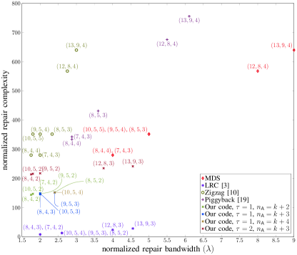
Figure 5: Comparisons of different $(n,k,f)$ codes with $\nu=8$.

In Figs. 5 and 6, we compare our codes with Construction $1$ for the Class ${\mathsf{B}}$ codes (i.e., the codes are constructed as shown in Sections III and IV) with other codes in the literature. We remark that the Pyramid codes in Fig. 6 refer to the basic Pyramid codes in [2], while the exact-repairable MDS codes refer to the $(2,n-k,n-1)$ exact-repairable MDS codes from [24, Sec. IV]. The aforementioned notation, unlike our notation in this paper, refers to an $(n,k,n-k)$ code that has $\lambda\leq 2\frac{n-1}{n-k}$, $\beta=n-k$, and repair locality of $n-1$. For generalized Piggyback codes [23], we choose $\beta=k$. Also note that the parameters $s,p$ are chosen according to [23, Eq. 20], i.e., $s=\left\lfloor k\frac{\sqrt{n-k}-1}{\sqrt{n-k}}\right\rfloor$ or $s=\left\lceil k\frac{\sqrt{n-k}-1}{\sqrt{n-k}}\right\rceil$ and $p=k-s$, whichever pair of values gives the lowest repair bandwidth. In case of a tie, the pair that gives the lowest repair complexity was chosen. In particular, the figure plots the normalized repair complexity of $(n,k,f)$ codes over $\text{GF}(2^{8})$ ($\nu=8$) versus their normalized repair bandwidth $\lambda$. In the figure, we show the exact repair bandwidth for our proposed codes, while the reported repair complexities and the repair bandwidths of the other codes, except for Piggyback, generalized Piggyback, and exact-repairable MDS codes, are from Table I. For Piggyback, generalized Piggyback, and exact-repairable MDS codes exact values for the repair bandwidth and the repair complexity are calculated directly from the codes. Furthermore, for a fair comparison we assume the parity symbols in the first parity node of all storage codes to be weighted sums. The only exception is the LRCs and the exact-repairable MDS codes, as the code design enforces the parity-check equations to be non-weighted sums. Thus, changing it would alter the maximum erasure correcting capability of the LRC and the repair bandwidth of the exact-repairable MDS code. We also assume that the LRCs and the Pyramid codes have a repair locality of $k/2$. For the generalized Piggyback codes, we assume that the codes have sub-packetization $\beta=k$. For the Piggyback codes, we consider the construction that repairs just the data nodes. Therefore, they have a sub-packetization of $2$.

TABLE II: Comparison of normalized repair complexity and bandwidth of $(n,k,f)$ BASIC PM-MBR codes [20] and the proposed codes.

Proposed	$n_{\mathsf{A}}$	$\tau$	$R$	$\mathrm{GF}(q)$	BASIC PM-MBR	$R^{\mathsf{b}}$	$\delta^{\mathsf{b}}$	$\mathcal{R}_{m}$	$C_{\mathsf{r}}^{\mathsf{b}}$	$C_{\mathsf{r}}$	$\lambda^{\mathsf{b}}$	$\lambda$
$(9,5,3)$	$8$	$1$	$0.5556$	$\mathrm{GF}(11)$	$(8,5,3)$	0.4464	$7$	$\mathcal{R}_{11}$	$135$	$44$	$1$	$2.4$
$(11,7,3)$	$10$	$2$	$0.6364$	$\mathrm{GF}(11)$	$(11,7,4)$	$0.4454$	$10$	$\mathcal{R}_{11}$	$187.5$	$66.2857$	$1$	$3$
$(14,9,3)$	$12$	$2$	$0.6428$	$\mathrm{GF}(13)$	$(14,9,5)$	$0.4450$	$13$	$\mathcal{R}_{17}$	$384$	$70.6667$	$1$	$3.5556$

The best codes for a DSS should be the ones that achieve the lowest repair bandwidth and have the lowest repair complexity. As seen in Fig. 5, MDS codes have both high repair complexity and repair bandwidth, but they are optimal in terms of fault tolerance for a given $n$ and $k$. Zigzag codes achieve the same fault tolerance and high repair complexity as MDS codes, but at the lowest repair bandwidth. At the other end, LRCs yield the lowest repair complexity, but a higher repair bandwidth and worse fault tolerance than Zigzag codes. Piggyback codes, generalized Piggyback codes, and exact-repairable MDS codes have a repair bandwidth between those of Zigzag and MDS codes, but with a higher repair complexity. Strictly speaking, they have a repair complexity higher than MDS codes. For a given storage overhead, our proposed codes have better repair bandwidth than MDS codes, Piggyback codes, generalized Piggyback codes, and exact-repairable MDS codes. In particular, the numerical results in Figs. 5 and 6 show that for different code parameters with $\tau=1$ and $n_{\mathsf{A}}-k=2$ our proposed codes yield a reduction of the repair bandwidth in the range of $64\%-50\%$, $39.13\%-30.43\%$, $43.04\%-33.33\%$, and $33.33\%-30\%$, respectively. Furthermore, our proposed codes yield lower repair complexity as compared to MDS, Piggyback, generalized Piggyback, exact-repairable MDS, and Zigzag codes. Again, the numerical analysis in Figs. 5 and 6 shows that for different code parameters with $\tau=1$ and $n_{\mathsf{A}}-k=2$ our proposed codes yield a reduction of the repair complexity in the range of $58.18\%-47.86\%$, $64.75\%-56.89\%$, $59.26\%-49.30\%$, $78.70\%-67.93\%$, and $58.18\%-47.86\%$, respectively. However, the benefits in terms of repair bandwidth and/or repair complexity with respect to MDS codes, Zigzag codes, and codes constructed using the piggybacking framework come at a price of a lower fault tolerance. For fixed $(n,k,f)$ it can be seen that the proposed codes yield a reduction of the repair bandwidth in the range of $7.69\%-0\%$ compared to LRCs and Pyramid codes, while in some cases, for the latter codes our proposed codes achieve a reduction of the repair complexity in the range of $24.44\%-15.18\%$.

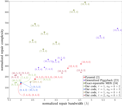
Figure 6: Comparisons of different $(n,k,f)$ codes with $\nu=8$.

In Table II, we compare the normalized repair complexity of the proposed codes with Construction $1$ for the Class ${\mathsf{B}}$ code and BASIC PM-MBR codes presented in [20]. BASIC PM-MBR codes are constructed from an algebraic ring $\mathcal{R}_{m}$, where each symbol in the ring is a binary vector of length $m$. In order to have a fair comparison with our codes, we take the smallest possible field size for our codes and the smallest possible ring size for the codes in [20]. Furthermore, to compare codes with similar storage overhead, we consider BASIC PM-MBR codes with repair locality, denoted by $\delta^{\mathsf{b}}$, that leads to the same file size as for our proposed codes (which is equal to $k^{2}$) and code length $n$ such that the code rate (which is the inverse of the storage overhead) is as close as possible to that of our proposed codes. The Class ${\mathsf{A}}$ codes of the proposed codes in the table are $(n_{\mathsf{A}},n_{\mathsf{A}}-f)$ RS codes. The codes are over $\text{GF}(n_{\mathsf{A}}+1)$ if $n_{\mathsf{A}}+1$ is a prime (or a power of a prime). If $n_{\mathsf{A}}+1$ is not a prime (or a power of prime), we construct an $(n^{\prime},n^{\prime}-f)$ RS code over $\mathrm{GF}(n^{\prime}+1)$, where $n^{\prime}+1$ is the smallest prime (or the smallest power of a prime) with $n^{\prime}+1\geq n_{\mathsf{A}}+1$, and then we shorten the RS code to obtain an $(n_{\mathsf{A}},n_{\mathsf{A}}-f)$ Class ${\mathsf{A}}$ code. In the table, the parameters for the proposed codes are given in columns $1$ to $5$ and those of the codes in [20] in columns $6$ to $9$. The code rates $R$ and $R^{\mathsf{b}}$ of the proposed codes and the BASIC PM-MBR codes are given in columns $4$ and $7$, respectively. The smallest possible field size for our codes and the smallest possible ring size for the BASIC PM-MBR codes are given in columns $5$ and $9$, respectively. The normalized repair complexity for BASIC PM-MBR codes, $C^{\mathsf{b}}_{\mathsf{r}}$, is given in column $10$, while the normalized repair complexity of the proposed codes, $C_{\mathsf{r}}$, is given in column $11$. The normalized repair bandwidth for BASIC PM-MBR codes, $\lambda^{\mathsf{b}}$, is given in column $12$, while the normalized repair bandwidth of the proposed codes, $\lambda$, is given in the last column. It can be seen that the proposed codes achieve significantly better repair complexity. However, this comes at the cost of a lower fault tolerance for the codes in rows $2$ and $3$ (but our codes have significantly higher code rate) and higher repair bandwidth (since BASIC PM-MBR codes are MBR codes, their normalized repair bandwidth is equal to $1$). For the $(9,5,3)$ code, the same fault tolerance of the $(8,5,3)$ code in [20] is achieved, despite the fact that the proposed code has a higher code rate. We remark that FR codes achieve a better (trivial) repair complexity compared to our proposed codes. However, this comes at a cost of $R<0.5$ and they cannot be constructed for any $n$, $k$, and $\delta$, where $\delta$ is the repair locality.

In Table III, we compare the normalized repair bandwidth of the proposed codes using Construction $1$ and Construction $2$ for Class ${\mathsf{B}}$ nodes. In the table, with $\lambda^{\mathsf{C}1}$ and $\lambda^{\mathsf{C}2}$, we refer to the normalized repair bandwidth for Construction $1$ and Construction $2$, respectively. For the codes presented, it is seen that the heuristic construction yields an improvement in repair bandwidth in the range of $1\%-7\%$ with respect to Construction $1$.

TABLE III: Improvement in normalized repair bandwidth of the proposed $(n,k)$ codes when the Class ${\mathsf{B}}$ nodes are heuristically constructed.

Code	$n_{\mathsf{A}}$	$\tau$	$\lambda^{{\mathsf{C}}1}$	$\lambda^{{\mathsf{C}}2}$	Improvement
$(7,4)$	$6$	$1$	$2$	$1.875$	$6.25\%$
$(10,6)$	$9$	$2$	$2.5$	$2.4167$	$3.33\%$
$(13,8)$	$12$	$3$	$3$	$2.9375$	$2.08\%$
$(14,8)$	$12$	$3$	$2.375$	$2.3125$	$2.63\%$
$(16,10)$	$15$	$4$	$3.5$	$3.45$	$1.43\%$

VII Conclusion

In this paper, we constructed a new class of codes that achieve low repair bandwidth and low repair complexity for a single node failure. The codes are constructed from two smaller codes, Class ${\mathsf{A}}$ and ${\mathsf{B}}$, where the former focuses on the fault tolerance of the code, and the latter focuses on reducing the repair bandwidth and complexity. It is numerically seen that our proposed codes achieve better repair complexity than Zigzag codes, MDS codes, Piggyback codes, generalized Piggyback codes, exact-repairable MDS codes, BASIC PM-MBR codes, and are in some cases better than Pyramid codes. They also achieve a better repair bandwidth compared to MDS codes, Piggyback codes, generalized Piggyback codes, exact-repairable MDS codes, and are in some cases better than LRCs and Pyramid codes. A side effect of such a construction is that the number of symbols per node that need to be encoded grows only linearly with the code dimension. This implies that our codes are suitable for memory constrained DSSs as compared to Zigzag and MDR codes, for which the number of symbols per node increases exponentially with the code dimension.

Appendix A Proof of Theorem 1

Consider an arbitrary set of $\tau^{\prime}\leq\tau$ piggybacked nodes, denoted by $\mathcal{T}=\{j_{1},j_{2},\ldots,j_{\tau^{\prime}}\}$, $j_{i}=j^{\prime}_{i}-(n_{\mathsf{A}}-\tau)+1$, $j^{\prime}_{i}\in\{n_{\mathsf{A}}-\tau,\ldots,n_{\mathsf{A}}-1\}$. Then, the repair of the $i$-th row, $i=0,\ldots,k-1$, using the piggybacked nodes in $\mathcal{T}$, would depend upon the knowledge of the data symbols (piggybacks) in the rows $(i+j_{1})_{k},(i+j_{2})_{k},\ldots,(i+j_{\tau^{\prime}})_{k}$. This is because the knowledge of the piggybacks in these rows allows to obtain the original MDS parity symbols in the $i$-th row. In the following, we use this observation. We first proceed to prove that if $\tau^{\prime}(\tau^{\prime}+n_{\mathsf{A}}-k-\tau)<k$, then $\theta+\tau^{\prime}\leq n_{\mathsf{A}}-k-\tau+\tau^{\prime}$ data nodes can be corrected using $\theta$ non-modified parity nodes and the $\tau^{\prime}$ piggybacked nodes in $\mathcal{T}$. Using this we will complete the proof of Theorem 1.

Lemma 1

Consider an $(n_{\mathsf{A}},k)$ Class ${\mathsf{A}}$ code with $k+2\leq n_{\mathsf{A}}<2k$. The code consists of $\tau$ piggybacked nodes and $n_{\mathsf{A}}-k-\tau$ non-modified MDS parity nodes. If $\tau^{\prime}(\tau^{\prime}+n_{\mathsf{A}}-k-\tau)<k$, then the code can correct $\theta+\zeta$ data node failures using $\theta\leq n_{\mathsf{A}}-k-\tau$ non-modified parity nodes and the $\tau^{\prime}$ piggybacked parity nodes in the set $\mathcal{T}=\{1,\ldots,\tau^{\prime}\}$ for $\zeta\leq\tau^{\prime}\leq\tau$.

Proof:

We consider first the case when $\zeta=\tau^{\prime}$. Then, assume that $\theta+\zeta$ data nodes fail and there exists a sequence $i,(i+1)_{k},\ldots,(i-1+\tau^{\prime})_{k}$ of $\tau^{\prime}$ data nodes that are available. By construction, the parity symbol $p^{{\mathsf{A}},\mathsf{p}}_{(j-1)_{k},n_{\mathsf{A}}-\tau-1+t}$, $t\in\mathcal{T}$, is (see (3)) given by

$$p^{{\mathsf{A}},\mathsf{p}}_{(j-1)_{k},n_{\mathsf{A}}-\tau-1+t}=p^{{\mathsf{A}}}_{(j-1)_{k},n_{\mathsf{A}}-\tau-1+t}+d_{(j-1+t)_{k},(j-1)_{k}},$$ (11)

where $j=0,\ldots,k-1$. To recover all data symbols, set $i^{\prime}=(i+\tau^{\prime})_{k}$ and perform the following steps.

1. Obtain the $\zeta=\tau^{\prime}$ MDS parity symbols $p^{\mathsf{A}}_{(i^{\prime}-1)_{k},n_{\mathsf{A}}-\tau-1+t}$, $t\in\mathcal{T}$ (see (11)) in the $(i^{\prime}-1)_{k}$-th row. This is possible because the piggybacks in the $(i^{\prime}-1)_{k}$-th node are available.

2. Using the $\theta+\zeta$ MDS parity symbols and $k-\theta-\zeta$ data symbols in the $(i^{\prime}-1)_{k}$-th row, recover the missing $\theta+\zeta$ symbols in the $(i^{\prime}-1)_{k}$-th row of the failed data nodes.

3. $i^{\prime}\leftarrow(i^{\prime}-1)_{k}$.

4. Repeat Items 1), 2), and 3) $\tau^{\prime}-1$ times. This ensures that the failed symbols in the $\tau^{\prime}$ rows $i^{\prime},(i^{\prime}+1)_{k},\ldots,(i^{\prime}-1+\tau^{\prime})_{k}$ are recovered. This implies that the piggyback symbols

   $$\begin{split}&d_{i^{\prime},(i^{\prime}-1)_{k}},\ldots,d_{(i^{\prime}-1+\tau^{\prime})_{k},(i^{\prime}-1)_{k}}\,\,\text{in node}\,\,(i^{\prime}-1)_{k},\\ &d_{i^{\prime},(i^{\prime}-2)_{k}},\ldots,d_{(i^{\prime}-2+\tau^{\prime})_{k},(i^{\prime}-2)_{k}}\,\,\text{in node}\,\,(i^{\prime}-2)_{k},\\ &\,\,\,\,\,\,\,\,\,\,\,\,\,\,\,\,\,\,\,\,\,\,\,\,\,\,\,\,\,\vdots\\ &d_{i^{\prime},(i^{\prime}-\tau^{\prime})_{k}}\,\,\,\,\,\,\,\,\,\,\,\,\,\,\,\,\,\,\,\,\,\,\,\,\,\,\,\,\,\,\,\,\,\,\,\,\,\,\,\,\,\,\,\,\,\,\,\,\,\,\,\,\,\,\,\,\text{in node}\,\,(i^{\prime}-\tau^{\prime})_{k},\end{split}$$ (12)

   are recovered. In other words,  12 says that in the $(i^{\prime}-t)_{k}$-th node, $\tau^{\prime}+1-t$ piggybacked symbols are recovered. More specifically, for $t=1$, $\tau^{\prime}$ piggybacked symbols are recovered. Thus,

5. repeat Items 1) and 2), and set

6. $i^{\prime}\leftarrow(i^{\prime}-1)_{k}$. We thus recover the $i^{\prime}$-th row and obtain the piggyback symbols in $\mathcal{D}_{\mathcal{R}_{i^{\prime}}}\backslash\mathcal{D}_{\mathcal{X}_{i^{\prime}}}$. This increases the number of obtained piggyback symbols by $1$ in the next $\tau^{\prime}$ nodes $i^{\prime},(i^{\prime}-1)_{k},\ldots,(i^{\prime}+\tau^{\prime}-1)_{k}$. In a similar fashion, we now have $\tau^{\prime}$ piggybacked symbols in the $i^{\prime}$-th node, and Items 5) and 6) are repeated until all $k$ rows have been recovered. With this recursion, one recovers the $\theta+\tau^{\prime}=\theta+\zeta$ failed data nodes.

For the case when $\zeta<\tau^{\prime}$, the aforementioned decoding procedure is still able recover $\theta+\zeta$ data node failures. This is because, in order to repair failed symbols in the $(i^{\prime}-1)_{k}$-th row, one needs just $\zeta<\tau^{\prime}$ MDS parity symbols from $\mathcal{T}^{\prime}\subseteq\mathcal{T}$. If the $(i^{\prime}-1)_{k}$-th node is available, then $\zeta$ piggybacks allow to recover the MDS parity symbols (see Item 1)). On the contrary, if the $(i-1)_{k}$-th node has been erased, then $\zeta$ piggybacks are obtained from  12.

Note that the argument above assumes that $\tau^{\prime}$ consecutive data nodes are available. Thus, in order to guarantee that any $\theta+\zeta$ data nodes can be corrected, we consider the worst case scenario for node failures, where we equally spread $\theta+\zeta$ data node failures across the $k$ data nodes. Since

$$\frac{k}{\theta+\zeta}\geq\frac{k}{n_{\mathsf{A}}-k-\tau+\tau^{\prime}}>\tau^{\prime},$$

where the last inequality follows by the assumption on $\tau^{\prime}$ stated in the lemma, it follows that the largest gap of non-failed data nodes in the worst case scenario is indeed greater than or equal to $\tau^{\prime}$. ∎

The above lemma shows that the Class ${\mathsf{A}}$ code can correct up to $n_{\mathsf{A}}-k-\tau+\tau^{\prime}$ erasures using non-modified parity nodes and $\tau^{\prime}$ modified parity nodes, provided the condition on $\tau^{\prime}$ is satisfied.

To prove that the code can correct $n_{\mathsf{A}}-k-\tau+\tau^{\prime}$ arbitrary node failures, let us assume that $\rho$ Class ${\mathsf{A}}$ parity nodes and $n_{\mathsf{A}}-k-\tau+\tau^{\prime}-\rho$ data nodes have failed. More precisely, let $\rho_{1}\leq n_{\mathsf{A}}-k-\tau$ non-modified nodes, $\rho_{2}\leq\tau^{\prime}$ piggybacked nodes in $\mathcal{T}$, and $\rho_{3}\geq 0$ remaining piggybacked nodes, where $\rho_{1}+\rho_{2}+\rho_{3}=\rho$, fail. Clearly, it can be seen that there are $n_{\mathsf{A}}-k-\tau-\rho_{1}$ non-modified parity nodes and a set of $\zeta=\tau^{\prime}-\rho_{2}$ modified nodes $\mathcal{T}^{\prime}\subseteq\mathcal{T}$ available. Also, note that the number of data node failures is $\rho_{3}$ less than the number of combined available piggybacked nodes in $\mathcal{T}^{\prime}$ and available non-modified parity nodes. Thus, using Lemma 1 with $\theta=n_{\mathsf{A}}-k-\tau-\rho_{1}-\rho_{3}$ and $\zeta=\tau^{\prime}-\rho_{2}$, it follows that $\theta+\zeta=(n_{\mathsf{A}}-k-\tau-\rho_{1}-\rho_{3})+(\tau^{\prime}-\rho_{2})=n_{\mathsf{A}}-k-\tau+\tau^{\prime}-\rho$ data nodes can be repaired. The remaining $\rho$ failed parity nodes can then be repaired using the $k^{2}$ data symbols in the $k$ data nodes.

We remark that the decoding procedure in Lemma 1 in essence solves a system of linear equations by eliminating $\tau^{\prime}k$ variables (piggybacks) in $\tau^{\prime}$ parity nodes. Once the piggybacks are eliminated, the $k(\theta+\tau^{\prime})$ data symbols are obtained by solving $k$ systems of linear equations. Thus, the decoding procedure is optimal, i.e., it is maximum likelihood decoding.

Consider the quadratic function $\psi(\tau^{\prime})={\tau^{\prime}}^{2}+(n_{\mathsf{A}}-k-\tau)\tau^{\prime}-k$. According to the proof of Lemma 1 when $\psi(\tau^{\prime})\geq 0$, the decoding procedure fails as one can construct a failure pattern for the data nodes where the largest separation (in the number of available nodes) between the failed nodes would be strictly smaller than $\tau^{\prime}$. The largest $\tau^{\prime}$ such that $\psi(\tau^{\prime})<0$ can be determined as follows. By simple arithmetic, one can prove that $\psi(\tau^{\prime})$ is a convex function with a negative minima and with a positive and a negative root. Therefore,

$$0\leq\tau^{\prime}<\xi=\frac{\sqrt{(n_{\mathsf{A}}-k-\tau)^{2}+4k}-(n_{\mathsf{A}}-k-\tau)}{2},$$

where $\xi$ is the positive root of $\psi(\tau^{\prime})$. Furthermore, it may happen that $\tau<\xi$. Therefore, the maximum number of node failures that the code can tolerate is

$$f=\begin{cases}n_{\mathsf{A}}-k-\tau+\bigg{\lfloor}\frac{\sqrt{(n_{\mathsf{A}}-k-\tau)^{2}+4k}-(n_{\mathsf{A}}-k-\tau)}{2}\bigg{\rfloor}&\text{if}\,\,\tau\geq\xi\\ n_{\mathsf{A}}-k&\text{if}\,\,\tau<\xi\end{cases}.$$

Appendix B Class ${\mathsf{B}}$ Parity Node Construction

Initialization:

$\bm{A}=[a_{i,j}]$ as defined in (7)

$n=n_{\mathsf{A}}+n_{\mathsf{B}}-k$ with $n_{\mathsf{B}}<2k-\tau$ and $n_{\mathsf{A}}<2k$

1 for $l\in\{n_{\mathsf{A}},\ldots,n-1\}$ do

2       $\rho_{l}\leftarrow k-\tau-1-l+n_{\mathsf{A}}$

3       if $l\leq n_{\mathsf{A}}+k/2-\tau-2$ then

4             $\mathcal{P}^{{\mathsf{B}},\mathsf{h}}_{l}\leftarrow\mathcal{P}^{{\mathsf{B}}}_{l}$

5      else if $l>n_{\mathsf{A}}+k/2-\tau-2$ and $\rho_{l}>1$ then

6             $\mathcal{P}^{{\mathsf{B}},\mathsf{h}}_{l}\leftarrow$ ConstructNode($\bm{A},\rho_{l}$)

7      else if $l>n_{\mathsf{A}}+k/2-\tau-2$ and $\rho_{l}=1$ then

8             $\mathcal{P}^{{\mathsf{B}},\mathsf{h}}_{l}\leftarrow$ ConstructLastNode()

9       end if

10      $\bm{A}\leftarrow$ UpdateReadCost()

11 end for

Algorithm 1 Class ${\mathsf{B}}$ node construction when $k$ is even

In this appendix, we give an algorithm that constructs $n_{\mathsf{B}}-k$ Class ${\mathsf{B}}$ parity nodes $\mathcal{P}^{{\mathsf{B}},\mathsf{h}}_{n_{\mathsf{A}}},\ldots,\mathcal{P}^{{\mathsf{B}},\mathsf{h}}_{n-1}$. The algorithm is a heuristic for the construction of Class ${\mathsf{B}}$ parity nodes such that the repair bandwidth of failed nodes is further reduced in comparison with Construction $1$ in Section IV.

The nodes $\mathcal{P}^{{\mathsf{B}},\mathsf{h}}_{l}$, $l=n_{\mathsf{A}},\ldots,n-1$, are constructed recursively as shown in Algorithm 1. The $k$ parity symbols in the $l$-th node are sums of at most $\rho_{l}$ data symbols $d_{i,j}\in\cup_{j^{\prime}}\mathcal{D}_{\mathcal{Q}_{j^{\prime}}}$. The construction of the $l$-th node for $l\leq n_{\mathsf{A}}+k/2-\tau-2$ (see Algorithm 1) is identical to that resulting from Construction $1$ in Section IV. The remaining parity nodes $\mathcal{P}^{{\mathsf{B}},\mathsf{h}}_{l}$, $l>n_{\mathsf{A}}+k/2-\tau-2$, are constructed using the sub-procedures ConstructNode ($\bm{A},\rho_{l}$) and ConstructLastNode (  ). After the construction of each parity node, the read costs of the data symbols $d_{i,j}$ are updated by the sub-procedure UpdateReadCost (  ). In the following, we describe each of the above-mentioned sub-procedures.

B-A ConstructNode ($\bm{A},\rho_{l}$)

This sub-procedure allows the construction of the $l$-th Class ${\mathsf{B}}$ parity node, where each parity symbol in the node is a sum of at most $\rho_{l}$ data symbols. The algorithm for the sub-procedure is shown in Algorithm 2. Here, the algorithm is divided into two parts. The first part (Algorithm 2 to Algorithm 2) adds at most two data symbols to each of the $k$ parity symbols, while the second part (Algorithm 2 to Algorithm 2) adds at most $\rho_{l}-2$ data symbols.

In the first part, each parity symbol $p^{\mathsf{B}}_{t,l}$, $t=0,\ldots,k-1$, is recursively constructed by adding a symbol $d_{i,j}\in\mathcal{D}_{\mathcal{Q}_{j}\backslash\cup_{j^{\prime}}\mathcal{U}_{j^{\prime}}}$ which has a corresponding read cost $a_{i,j}$ that is the largest among all symbols indexed by $\mathcal{Q}_{j}\backslash\cup_{j^{\prime}}\mathcal{U}_{j^{\prime}}$ (see Algorithm 2 and Algorithm 2). The next symbol added to $p^{\mathsf{B}}_{t,l}$ is $d_{j,i}\in\mathcal{D}_{\mathcal{X}_{j}}$ if such a symbol exists (Algorithm 2). Otherwise, the symbol added is $d_{j,i_{2}}\in\mathcal{D}_{\mathcal{X}_{j}\backslash\cup_{j^{\prime}}\mathcal{U}_{j^{\prime}}}$ if such a symbol exists (Algorithm 2). The set $\mathcal{U}_{t}$ denotes the index set of data symbols from $\mathcal{D}$ that are added to $p^{\mathsf{B}}_{t,l}$. Note that there exist multiple choices for the symbol $d_{i,j}$. A symbol $d_{i,j}$ such that there is a valid $d_{j,i}\in\mathcal{D}_{\mathcal{X}_{j}}$ is preferred, since it allows a larger reduction of the repair bandwidth.

The second part of the algorithm chooses recursively at most $\rho_{l}-2$ data symbols that should participate in the construction of the $k$ parity symbols. The algorithm chooses a symbol $d_{j,i_{3}}\in\mathcal{D}_{\mathcal{X}_{j}\backslash\cup_{j^{\prime}}\mathcal{U}_{j^{\prime}}}\not=\emptyset$ such that $\operatorname*{read}(d_{j,i_{3}},p^{\mathsf{B}}_{t,l}+d_{j,i_{3}})<a_{j,i_{3}}$ (see Algorithm 2). In other words, choose data symbols such that their read cost do not increase. It may happen that $\mathcal{D}_{\mathcal{X}_{j}\backslash\cup_{j^{\prime}}\mathcal{U}_{j^{\prime}}}=\emptyset$. If so, select $d_{j_{2},i}\in\cup_{j_{1}}\mathcal{D}_{\mathcal{X}_{j_{1}}\backslash\cup_{j_{1}^{\prime}}\mathcal{U}_{j_{1}^{\prime}}}$ such that $d_{i^{\prime},j_{2}}\in\mathcal{D}_{\mathcal{U}_{t}}$ and $a_{j_{2},i}>1$, for some $i^{\prime}\neq i$, exists, and then add $d_{j_{2},i}$ to the parity symbol $p^{\mathsf{B}}_{t,l}$ (see Algorithm 2). If $d_{j_{2},i}$ does not exist, then an arbitrary symbol $d_{j_{3},i}\in\cup_{j_{1}}\mathcal{D}_{\mathcal{X}_{j_{1}}\backslash\cup_{j_{1}^{\prime}}\mathcal{U}_{j_{1}^{\prime}}}$ is added (see Algorithm 2). This process is then repeated $\rho_{l}-2$ times.

Initialization:

$t,j\leftarrow 0$

$\mathcal{U}_{t_{1}}\leftarrow\emptyset,\,\,\,\,\,t_{1}=0,\ldots,k-1$

1 while $\min_{\forall t_{1}}|\mathcal{U}_{t_{1}}|<2$ do

2       Select $d_{i,j}\in\mathcal{D}_{\Psi(\bm{A}_{\mathcal{Q}_{j}\backslash\cup_{j^{\prime}}\mathcal{U}_{j^{\prime}}})}$ s.t. $\exists\,d_{j,i}\in\mathcal{D}_{\mathcal{X}_{j}},a_{j,i}>1$

3       if $d_{i,j}$ exists then

4             $p^{\mathsf{B}}_{t,l}\leftarrow d_{i,j}+d_{j,i}$

5             $\mathcal{U}_{t}\leftarrow\mathcal{U}_{t}\cup\{(i,j),(j,i)\}$; $t\leftarrow t+1$

6      else

7             Select $d_{i_{1},j}\in\mathcal{D}_{\Psi(\bm{A}_{\mathcal{Q}_{j}\backslash\cup_{j^{\prime}}\mathcal{U}_{j^{\prime}}})}$

8             if $d_{i_{1},j}$ exists then

9                   if $\exists\,d_{j,i_{2}}\in\mathcal{D}_{\mathcal{X}_{j}\backslash\cup_{j^{\prime}}\mathcal{U}_{j^{\prime}}}$ s.t. $\operatorname*{read}(d_{j,i_{2}},p^{\mathsf{B}}_{t,l}+d_{j,i_{2}})<a_{j,i_{2}}$ and $a_{j,i_{2}}>1$ then

10                         $p^{\mathsf{B}}_{t,l}\leftarrow d_{i_{1},j}+d_{j,i_{2}}$

11                         $\mathcal{U}_{t}\leftarrow\mathcal{U}_{t}\cup\{(i_{1},j),(j,i_{2})\}$; $t\leftarrow t+1$

12                  else

13                         $p^{\mathsf{B}}_{t,l}\leftarrow d_{i_{1},j}$

14                         $\mathcal{U}_{t}\leftarrow\mathcal{U}_{t}\cup\{(i_{1},j),(-1,-1)\}$; $t\leftarrow t+1$

15                   end if

16                  

17             end if

18            

19       end if

20      $j\leftarrow(j+1)_{k}$

21 end while

22 $t,j\leftarrow 0$

23 while $\min_{\forall t_{1}}|\mathcal{U}_{t_{1}}|\leq\rho_{l}$ do

24       if $\mathcal{D}_{\mathcal{X}_{j}\backslash\cup_{j_{1}}\mathcal{U}_{j_{1}}}\not=\emptyset$ then

25             if $\exists\,d_{j,i_{3}}\in\mathcal{D}_{\mathcal{X}_{j}\backslash\cup_{j^{\prime}}\mathcal{U}_{j^{\prime}}}$ s.t. $\operatorname*{read}(d_{j,i_{3}},p^{\mathsf{B}}_{t,l}+d_{j,i_{3}})<a_{j,i_{3}}$ and $a_{j,i_{3}}>1$ then

26                   $p^{\mathsf{B}}_{t,l}\leftarrow p^{\mathsf{B}}_{t,l}+d_{j,i_{3}}$

27                   $\mathcal{U}_{t}\leftarrow\mathcal{U}_{t}\cup\{(j,i_{3})\}$; $t\leftarrow t+1$

28            else if $l>n_{\mathsf{A}}$ then

29                   $\mathcal{U}_{t}\leftarrow\mathcal{U}_{t}\cup(-1,-1)\}$; $t\leftarrow t+1$

30             end if

31            

32      else

33             if $|\mathcal{U}_{t}|\leq\rho_{l}-1$ then

34                   Select $d_{j_{2},i}\in\cup_{j_{1}}\mathcal{D}_{\mathcal{X}_{j_{1}}\backslash\cup_{j_{1}^{\prime}}\mathcal{U}_{j_{1}^{\prime}}}$ s.t. $d_{i^{\prime},j_{2}}\in\mathcal{D}_{\mathcal{U}_{t}}$ and $a_{j_{2},i}>1$ for some $i^{\prime}\neq i$

35                   if $d_{j_{2},i}$ exists then

36                         $p^{\mathsf{B}}_{t,l}\leftarrow p^{\mathsf{B}}_{t,l}+d_{j_{2},i}$

37                         $\mathcal{U}_{t}\leftarrow\mathcal{U}_{t}\cup\{(j_{2},i)\}$; $t\leftarrow t+1$

38                  else

39                         Select $d_{j_{3},i}\in\cup_{j_{1}}\mathcal{D}_{\mathcal{X}_{j_{1}}\backslash\cup_{j_{1}^{\prime}}\mathcal{U}_{j_{1}^{\prime}}}$

40                         $p^{\mathsf{B}}_{t,l}\leftarrow p^{\mathsf{B}}_{t,l}+d_{j_{3},i}$

41                         $\mathcal{U}_{t}\leftarrow\mathcal{U}_{t}\cup\{(j_{3},i)\}$; $t\leftarrow t+1$

42                   end if

43                  

44             end if

45            

46       end if

47      $j\leftarrow(j+1)_{k}$

48 end while

return $\{p^{\mathsf{B}}_{0,l},\ldots,p^{\mathsf{B}}_{k-1,l}\}$

Algorithm 2 ConstructNode $(\bm{A},\rho_{l})$

B-B ConstructLastNode (  )

This procedure constructs the $l$-th Class ${\mathsf{B}}$ parity node that has $\rho_{l}=1$. In other words, each parity symbol $p^{\mathsf{B}}_{t,l}$ is a data symbol $d_{i,j}\in\cup_{j^{\prime}}\mathcal{D}_{\mathcal{Q}_{j^{\prime}}}$. The procedure works as follows. First, initialize $\mathcal{U}_{t}$ to be the empty set for $t=0,\ldots,k-1$. Then, for $t=0,\ldots,k-1$, assign first the data symbol $d_{i,j}$ to the parity symbol $p^{\mathsf{B}}_{t,l}$, where $d_{i,j}\in\mathcal{D}_{\Psi(\bm{A}_{\cup_{j^{\prime}}\mathcal{Q}_{j^{\prime}}\setminus\cup_{t^{\prime}}\mathcal{U}_{t^{\prime}}})}$, and then subsequently add $(i,j)$ to $\mathcal{U}_{t}$. Note that for each iteration there may exist several choices for $d_{i,j}$, in which case we can pick one of these randomly.

B-C UpdateReadCost (  )

After the construction of the $l$-th node, we update the read costs of all data symbols $d_{i,j}\in\cup_{j^{\prime}}\mathcal{D}_{\mathcal{Q}_{j^{\prime}}}$. These updated values are used during the construction of the $(l+1)$-th node. The read cost updates for the parity symbol $p^{\mathsf{B}}_{t,l}$, $t=0,\ldots,k-1$, are

$$a_{i,j}=\operatorname*{read}(d_{i,j},p^{\mathsf{B}}_{t,l}),\,\,\,\forall d_{i,j}\in\mathcal{D}_{\mathcal{U}_{t}}.$$

References

- [1] J. Huang, X. Liang, X. Qin, P. Xie, and C. Xie, “Scale-RS: An efficient scaling scheme for RS-coded storage clusters,” IEEE Trans. Parallel and Distributed Systems, vol. 26, no. 6, pp. 1704–1717, Jun. 2015.
- [2] C. Huang, M. Chen, and J. Li, “Pyramid codes: Flexible schemes to trade space for access efficiency in reliable data storage systems,” in Proc. IEEE Int. Symp. Network Comput. and Appl. (NCA), Cambridge, MA, Jul. 2007.
- [3] C. Huang, H. Simitci, Y. Xu, A. Ogus, B. Calder, P. Gopalan, J. Li, and S. Yekhanin, “Erasure coding in Windows Azure storage,” in Proc. USENIX Annual Technical Conf., Boston, MA, Jun. 2012.
- [4] M. Sathiamoorthy, M. Asteris, D. Papailiopoulos, A. G. Dimakis, R. Vadali, S. Chen, and D. Borthakur, “XORing elephants: Novel erasure codes for big data,” in Proc. 39th Very Large Data Bases Endowment (VLDB), Trento, Italy, Aug. 2013.
- [5] D. S. Papailiopoulos and A. G. Dimakis, “Locally repairable codes,” IEEE Trans. Inf. Theory, vol. 60, no. 10, pp. 5843–5855, Oct. 2014.
- [6] A. G. Dimakis, P. B. Godfrey, Y. Wu, M. J. Wainwright, and K. Ramchandran, “Network coding for distributed storage systems,” IEEE Trans. Inf. Theory, vol. 56, no. 9, pp. 4539–4551, Sep. 2010.
- [7] K. V. Rashmi, N. B. Shah, and P. V. Kumar, “Optimal exact-regenerating codes for distributed storage at the MSR and MBR points via a product-matrix construction,” IEEE Trans. Inf. Theory, vol. 57, no. 8, pp. 5227–5239, Aug. 2011.
- [8] S. El Rouayheb and K. Ramchandran, “Fractional repetition codes for repair in distributed storage systems,” in Proc. 48th Annual Allerton Conf. Commun., Control, and Comput., Monticello, IL, Sep./Oct. 2010.
- [9] Y. Wang, X. Yin, and X. Wang, “MDR codes: A new class of RAID-6 codes with optimal rebuilding and encoding,” IEEE J. Sel. Areas Commun., vol. 32, no. 5, pp. 1008–1018, May 2014.
- [10] I. Tamo, Z. Wang, and J. Bruck, “Zigzag codes: MDS array codes with optimal rebuilding,” IEEE Trans. Inf. Theory, vol. 59, no. 3, pp. 1597–1616, Mar. 2013.
- [11] V. R. Cadambe, C. Huang, J. Li, and S. Mehrotra, “Polynomial length MDS codes with optimal repair in distributed storage,” in Proc. 45th Asilomar Conf. Signals, Syst. and Comput. (ASILOMAR), Pacific Grove, CA, Nov. 2011.
- [12] G. K. Agarwal, B. Sasidharan, and P. V. Kumar, “An alternate construction of an access-optimal regenerating code with optimal sub-packetization level,” in Proc. 21st Nat. Conf. Commun. (NCC), Mumbai, India, Feb. 2015.
- [13] J. Li, X. Tang, and U. Parampalli, “A framework of constructions of minimal storage regenerating codes with the optimal access/update property,” IEEE Trans. Inf. Theory, vol. 61, no. 4, pp. 1920–1932, Apr. 2015.
- [14] Z. Wang, I. Tamo, and J. Bruck, “Explicit minimum storage regenerating codes,” IEEE Trans. Inf. Theory, vol. 62, no. 8, pp. 4466–4480, Aug. 2016.
- [15] B. Sasidharan, M. Vajha, and P. V. Kumar, “An explicit, coupled-layer construction of a high-rate MSR code with low sub-packetization level, small field size and all-node repair,” Sep. 2016, arXiv: 1607.07335v3. [Online]. Available: https://arxiv.org/abs/1607.07335
- [16] M. Ye and A. Barg, “Explicit constructions of optimal-access MDS codes with nearly optimal sub-packetization,” IEEE Trans. Inf. Theory, vol. 63, no. 10, pp. 6307–6317, Oct. 2017.
- [17] J. Li, X. Tang, and C. Tian, “A generic transformation for optimal repair bandwidth and rebuilding access in MDS codes,” in Proc. IEEE Int. Symp. Inf. Theory (ISIT), Aachen, Germany, Jun. 2017.
- [18] N. Raviv, N. Silberstein, and T. Etzion, “Constructions of high-rate minimum storage regenerating codes over small fields,” IEEE Trans. Inf. Theory, vol. 63, no. 4, pp. 2015–2038, Apr. 2017.
- [19] K. V. Rashmi, N. B. Shah, and K. Ramchandran, “A piggybacking design framework for read-and download-efficient distributed storage codes,” IEEE Trans. Inf. Theory, vol. 63, no. 9, pp. 5802–5820, Sep. 2017.
- [20] H. Hou, K. W. Shum, M. Chen, and H. Li, “BASIC codes: Low-complexity regenerating codes for distributed storage systems,” IEEE Trans. Inf. Theory, vol. 62, no. 6, pp. 3053–3069, Jun. 2016.
- [21] H. Hou, P. P. C. Lee, Y. S. Han, and Y. Hu, “Triple-fault-tolerant binary MDS array codes with asymptotically optimal repair,” in Proc. IEEE Int. Symp. Inf. Theory (ISIT), Aachen, Germany, Jun. 2017.
- [22] S. Kumar, A. Graell i Amat, I. Andriyanova, and F. Brännström, “A family of erasure correcting codes with low repair bandwidth and low repair complexity,” in Proc. IEEE Global Commun. Conf. (GLOBECOM), San Diego, CA, Dec. 2015.
- [23] S. Yuan and Q. Huang, “Generalized piggybacking codes for distributed storage systems,” in Proc. IEEE Global Commun. Conf. (GLOBECOM), Washington, DC, Dec. 2016.
- [24] A. S. Rawat, I. Tamo, V. Guruswami, and K. Efremenko, “MDS code constructions with small sub-packetization and near-optimal repair bandwidth,” IEEE Trans. Inf. Theory, to appear.
- [25] M. Blaum, J. Brady, J. Bruck, and J. Menon, “EVENODD: An efficient scheme for tolerating double disk failures in RAID architectures,” IEEE Trans. Comput., vol. 44, no. 2, pp. 192–202, Feb. 1995.
- [26] A. Karatsuba and Y. Ofman, “Multiplication of multidigit numbers on automata,” Sov. Phys. Doklady, vol. 7, no. 7, pp. 595–596, Jan. 1963.
- [27] A. Weimerskirch and C. Paar, “Generalizations of the Karatsuba algorithm for efficient implementations,” Jul. 2006. [Online]. Available: https://eprint.iacr.org/2006/224.pdf
- [28] J. M. Pollard, “The fast Fourier transform in a finite field,” Math. Comput., vol. 25, no. 114, pp. 365–374, Apr. 1971.
- [29] R. Crandall and C. Pomerance, Prime Numbers: A Computational Perspective. Springer, 2001.
- [30] S. Gao and T. Mateer, “Additive fast Fourier transforms over finite fields,” IEEE Trans. Inf. Theory, vol. 56, no. 12, pp. 6265–6272, Dec. 2010.