An FFT-based algorithm for efficient computation of Green’s functions for the Helmholtz and Maxwell’s equations in periodic domains

Abstract

The integral equation method is widely used in numerical simulations of 2D/3D acoustic and electromagnetic scattering problems, which needs a large number of values of the Green’s functions. A significant topic is the scattering problems in periodic domains, where the corresponding Green’s functions are quasi-periodic. The quasi-periodic Green’s functions are defined by series that converge too slowly to be used for calculations. Many mathematicians have developed several efficient numerical methods to calculate quasi-periodic Green’s functions. In this paper, we will propose a new FFT-based fast algorithm to compute the 2D/3D quasi-periodic Green’s functions for both the Helmholtz equations and Maxwell’s equations. The convergence results and error estimates are also investigated in this paper. Further, the numerical examples are given to show that, when a large number of values are needed, the new algorithm is very competitive.

Keywords: FFT-based algorithm, periodic domain, Green’s function, interpolation, convergence

1 Introduction

In the scattering theory, the integral equation method is an efficient and widely used method for numerical simulations. During the numerical procedure to solve the integral equations, a large number of values of the Green’s functions and their derivatives are needed. In recent years, many mathematicians are interested in the topic that the acoustic/electromagnetic fields scattered in periodic domains with quasi-periodic incident waves, where the corresponding Green’s functions are quasi-periodic. In this case, the quasi-periodic Green’s functions, that are defined by slowly convergent series, are always very difficult to evaluate. In this paper, we will develop a new FFT-based method to calculate the Green’s functions in 2D periodic domains or 3D doubly periodic domains for the Helmholtz equations and Maxwell’s equations numerically.

1) The quasi-periodic Green’s function $G(x)$ for Helmholtz equations in 2D domains.

Assume that the 2D domain is $2\pi$-periodic in $x_{1}$-direction, and the incident wave $u^{i}$ is $\alpha$-quasi-periodic, i.e., $u^{i}(x_{1}+2\pi,x_{2})=e^{i2\pi\alpha}u^{i}(x_{1},x_{2})$. The corresponding Green’s function is also $\alpha$-quasi-periodic and can be defined by the basic image expansion

$$G(x)=\frac{i}{4}H_{0}^{(1)}(k|x|)+\frac{i}{4}\sum_{n\neq 0,\,n\in{\mathbb{Z}}}e^{i2\pi\alpha n}H_{0}^{(1)}(kr_{n}),$$ (1.1)

where $r_{n}=\sqrt{(x_{1}-2\pi n)^{2}+x_{2}^{2}}$. It can also be defined by the basic eigenfunction expansion [14]:

$$G(x)=\frac{i}{4\pi}\sum_{n=-\infty}^{\infty}\frac{1}{\beta_{n}}\exp({i\alpha_{n}x_{1}+i\beta_{n}|x_{2}|}),$$ (1.2)

where $\alpha_{n}=\alpha+n$,

$$\beta_{n}=\begin{cases}\sqrt{k^{2}-\alpha_{n}^{2}},\quad&\text{if $|\alpha_{n}|\leq k$,}\\ i\sqrt{\alpha_{n}^{2}-k^{2}},\quad&\text{otherwise.}\end{cases}$$

2) The doubly quasi-periodic Green’s function $G_{d}(x)$ for Helmholtz equations in 3D domains.

Assume that the 3D domain is $2\pi$-periodic in both $x_{1}$- and $x_{2}$-directions, and the incident wave $u^{i}$ is doubly quasi-periodic, i.e., for any integers $m_{1},\,m_{2}$, $u^{i}(x_{1}+2m_{1}\pi,x_{2}+2m_{2}\pi,x_{3})=e^{i2m_{1}\pi\alpha_{1}}e^{i2m_{2}\pi\alpha_{2}}u^{i}(x_{1},x_{2},x_{3})$. Then the corresponding Green’s function is also doubly quasi-periodic and can be defined by the basic eigenfunction expansion [16]:

$$G_{d}(x)=\frac{i}{8\pi^{2}}\sum_{n_{1},n_{2}\in\mathbb{Z}}\frac{1}{\beta_{n_{1},n_{2}}}\exp(i\alpha_{1,n_{1}}x_{1}+i\alpha_{2,n_{2}}x_{2}+i\beta_{n_{1},n_{2}}|x_{3}|),$$ (1.3)

where $\alpha_{1},\,\alpha_{2}\in\mathbb{R}$, $\alpha_{1,n_{1}}=\alpha_{1}+n_{1}$, $\alpha_{2,n_{2}}=\alpha_{2}+n_{2},$

$$\beta_{n_{1},n_{2}}=\begin{cases}\sqrt{k^{2}-\alpha_{1,n_{1}}^{2}-\alpha_{2,n_{2}}^{2}},\quad&\text{if $\alpha_{1,n_{1}}^{2}+\alpha_{2,n_{2}}^{2}\leqslant k^{2}$,}\\ i\sqrt{\alpha_{1,n_{1}}^{2}+\alpha_{2,n_{2}}^{2}-k^{2}},\quad&\text{otherwise.}\end{cases}$$

3) The doubly quasi-periodic Green’s tensor $\mathbb{G}(x)$ for Maxwell’s equations in 3D domains.

The doubly quasi-periodic Green’s tensor $\mathbb{G}(x)$ for Maxwell equations is a $3\times 3$ matrix defined by $G_{d}(x)$:

$$\mathbb{G}(x)=G_{d}(x)\mathbb{I}+\frac{1}{k^{2}}\nabla\nabla\cdot(G_{d}(x)\mathbb{I}),$$ (1.4)

where $\mathbb{I}$ is the $3\times 3$ identity matrix. $\mathbb{G}(x)$ is composed of $G_{d}(x)$ and its second order derivatives. So the numerical method of $\mathbb{G}$ comes directly from that of $G_{d}(x)$.

In this paper, we will consider numerical methods to calculate the functions $G(x)$, $G_{d}(x)$ and $\mathbb{G}(x)$ in 2D/3D domains. We always assume that the cases we considered are away from Wood anomalies, i.e., $\beta_{n}\neq 0$ for the 2D case and $\beta_{n_{1},n_{2}}\neq 0$ for the 3D case. The definition (1.1) is the sum of Hankel functions that converges very slowly, which will cost a lot of time in calculation. From the definition of $G(x)$ in (1.2), the function $G(x)$ is defined by the series of exponential functions and converges rapidly when $x$ is away from the line $x_{2}=0$. When $x_{2}\rightarrow 0$, the series converges slowly, so this method fails. Similarly, the direct calculation from the definition (1.3) of $G_{d}(x)$ fails when $x_{3}\rightarrow 0$.

Many methods have been developed to evaluate the Green’s function in 2D and 3D domains, such as the Kummer’s transformation, the Ewald method, the Lattice sums and the integral representations. Linton compared several methods in 2D domains in [14] and in 3D domains in [16]. In these two papers, Linton gave the conclusions that, if only a few values are needed, the Ewald’s method is the most efficient method, while if a large number of values are needed, the lattice sums method is better. There are many papers concerning the lattice sums method and the Ewald’s method; see [9, 30, 23, 5, 20, 28, 1, 11, 21, 26] for the 2D case and [18, 6, 11, 21, 26, 20, 28, 20, 15, 25, 17] for the 3D case. There are also some other methods considering the numerical evaluation of the Green’s functions; see, e.g., [2, 22, 3, 4]. In particular, the cases that are near or at the Wood anomalies, which are very difficult to dealt with, have been considered in [22, 3, 4]. For very large $k$’s ($>10^{5}$), Kurkcu and Reitich introduced the NA method in 2D domains, which comes from the integral representations (see [10]). However, all of the known methods have their advantages and limitations. Take the lattice sums, the Ewald method and the NA method in 2D domain for example. The lattice sums converge very fast, especially when the wave number $k$ is small enough. This makes it the best method to calculate a large number of values in this case. But the convergence radius of the lattice sums depends on the wave number $k$. If $k$ becomes larger, the lattice sums need more terms to achieve the same accuracy, which involves more evaluations of Hankel functions and Bessel functions and thus needs more time. What is worse, when $k$ is getting larger ($k\geqslant 50$), the lattice sums only converge in a very small disk, so the method no longer works for most points. However, the Ewald’s method is always able to achieve the expected accuracy for both small and large $k$’s, but it costs much more time. So it might not be a good choice when a large number of values are needed. The NA method for 2D domains is of higher efficiency than the other methods when $k$ is very large ($>10^{5}$). However, when $k$ is not so large, e.g., $k\sim 100$, its efficiency is even worse than the Ewald method, so it is not suitable for the calculation. The aim of this paper is to seek for a more efficient method that converges for any wave number $k$. In this paper, we develop a new FFT-based method that converges for any $k$ and is very efficient when a large number of values are needed.

Our method is based on FFT. First, we will transform the Green’s function $G(x)$ ($G_{d}(x)$) into a periodic function in 2D (3D) domains. Then we can compute its Fourier series analytically by direct calculations. The idea is from [27], in which the Fourier series of the Hankel function are used to solve Lippmann-Schwinger equations in 2D domains. The method was extended to 2D periodic domains in [24] and to 3D domains in [8, 12]. In one periodic cell, $x=0$ is the only singularity of the Green’s function, where the Fourier series do not converge. For a better convergence, we will remove the singularity to get the smooth enough modified functions. The Fourier coefficients of the modified functions are computed numerically and applied to obtain the values on the grid points from IFFT. Then the values of the modified functions on random points can be evaluated simply by interpolation. It is now easy to obtain the values of the Green’s functions. The derivatives of the Green’s functions can be calculated in the similar way.

This paper is organized as follows. In Section 2, we give a new FFT-based algorithm to calculate the Green’s function $G(x)$ in two dimensions. In Section 3, the FFT-based algorithm is applied to calculate the Green’s function $G_{d}(x)$ for the Helmholtz equation in three dimensions. In Section 4, the FFT-based algorithm is extended to calculate the Green’s tensor $\mathbb{G}(x)$ for the Maxwell equations. The convergence analysis and error estimates are given in Section 5 for the numerical methods. In Section 6, we present some numerical examples for the calculation of $G(x),\,G_{d}(x),\,\mathbb{G}(x)$.

2 The FFT-based algorithm in two dimensions

2.1 Periodization and Fourier coefficients

Set $D_{c}=[-\pi,\pi]\times[-c,c]$, where $c$ is a positive real number which is chosen so that for $|x_{2}|\geq c$ the series expansion (1.2) can be directly used to compute $G(x)$ efficiently. Thus, we will develop an efficient method to compute the Green’s function $G(x)$ for $x\in D_{c}$.

From the series expansion (1.2) it follows that

$$e^{-i\alpha x_{1}}G(x)=\frac{i}{4\pi}\sum_{n=-\infty}^{\infty}\frac{1}{\beta_{n}}\exp({inx_{1}+i\beta_{n}|x_{2}|}),$$

which is $2\pi$-periodic in the $x_{1}$-direction.

Let $\widetilde{c}>c$ and let $\mathcal{X}(t)$ be a smooth cut-off function for $t\in{\mathbb{R}}$ such that $\mathcal{X}(t)=1$ for $|t|\leq c$ and $\mathcal{X}(t)=0$ for $|t|\geq(c+\widetilde{c})/2.$ Define a new function $K(x)$:

$$K(x)=e^{-i\alpha x_{1}}G(x)\mathcal{X}(|x_{2}|)\quad\mbox{for}\;x\in{\mathbb{R}}\times[-\widetilde{c},\widetilde{c}].$$

Then $K(x)$ is zero for $x\in[-\pi,\pi]\times[(c+\widetilde{c})/2,\widetilde{c}]$ and $x\in[-\pi,\pi]\times[-\widetilde{c},-(c+\widetilde{c})/2]$. We extend $K$ into a $2\widetilde{c}$-periodic function in $x_{2}$-direction which is denoted by $K$ again. Then $K$ is now a bi-periodic function in ${\mathbb{R}}^{2}$. Note that $K$ is smooth in $D_{\tilde{c}}\setminus\{0\}$ and

$$G(x)=e^{i\alpha x_{1}}K(x)\quad\text{for}\;\;x\in D_{c}.$$

We now calculate the Fourier coefficients of $K$. To do this, we divide the rectangular domain $D_{\widetilde{c}}$ uniformly into $2N\times 2N$ small rectangles. Set $S_{N}=\{j=(j_{1},j_{2})\in{\mathbb{Z}}^{2}\;:\;-N\leq j_{1},j_{2}<N\}$. The grid points are denoted by $x_{j}=(x_{1j_{1}},x_{2j_{2}})$, where $x_{1j_{1}}=(\pi/N)j_{1}$, $x_{2j_{2}}=(\widetilde{c}/N)j_{2}$ with $j=(j_{1},j_{2})\in S_{N}$. Define the Fourier basis of $L^{2}(D_{\widetilde{c}})$ by

$$\phi_{j}(x)=\frac{1}{2\sqrt{\pi\widetilde{c}}}\exp(ij_{1}x_{1}+ij_{2}\pi x_{2}/\widetilde{c}),\quad j=(j_{1},j_{2})\in{\mathbb{Z}}^{2}.$$

Then $K(x)$ can be approximated by $K_{N}(x)$:

$$K_{N}(x)=\sum_{j\in S_{N}}\hat{K}_{j}\phi_{j}(x),$$

where $\hat{K}_{j}$ is the j-th Fourier coefficient of $K$. By a direct calculation $\hat{K}_{j}$ is given by

$$\hat{K}_{j} = \int_{D_{\widetilde{c}}}K(x)\overline{\phi}_{j}(x)dx=\int_{D_{\widetilde{c}}}K(x)\phi_{-j}(x)dx$$

$$= \frac{i}{4\sqrt{\pi\widetilde{c}}}\frac{1}{\beta_{j_{1}}}\left(\int_{0}^{\widetilde{c}}e^{i(\beta_{j_{1}}-j_{2}\pi/\widetilde{c})x_{2}}\mathcal{X}(x_{2})dx_{2}+\int_{0}^{\widetilde{c}}e^{i(\beta_{j_{1}}+j_{2}\pi/\widetilde{c})x_{2}}\mathcal{X}(x_{2})dx_{2}\right).$$

If $\beta_{j_{1}}\neq\pm j_{2}\pi/\widetilde{c}$, then by integration by parts we have

$$\hat{K}_{j} = \frac{1}{2\sqrt{\pi\widetilde{c}}}\left[\frac{1}{(\alpha+j_{1})^{2}+(j_{2}\pi/\widetilde{c})^{2}-k^{2}}+\frac{1}{2\beta_{j_{1}}(j_{2}\pi/\widetilde{c}-\beta_{j_{1}})}\int_{0}^{\widetilde{c}}e^{i\beta_{j}x_{2}}\mathcal{X}^{\prime}(x_{2})e^{-i(j_{2}\pi/\widetilde{c})x_{2}}dx_{2}\right.$$ (2.1)

$$\left.\qquad-\frac{1}{2\beta_{j_{1}}(j_{2}\pi/\widetilde{c}+\beta_{j_{1}})}\int_{0}^{\widetilde{c}}e^{i\beta_{j}x_{2}}\mathcal{X}^{\prime}(x_{2})e^{i(j_{2}\pi/\widetilde{c})x_{2}}dx_{2}\right].$$

The last two integrals can be calculated by the one-dimensional Fast Fourier Transform (FFT) and matrix computation.

If $\beta_{j_{1}}=-j_{2}\pi/\widetilde{c}$ with $j_{2}\not=0$ then we have

$$\hat{K}_{j}=\frac{i}{4\sqrt{\pi\widetilde{c}}}\frac{1}{\beta_{j_{1}}}\int_{0}^{\widetilde{c}}\mathcal{X}(x_{2})dx_{2}+\frac{1}{4\sqrt{\pi\widetilde{c}}\beta_{j_{1}}(j_{2}\pi/\widetilde{c}-\beta_{j_{1}})}\left[1+\int_{0}^{\widetilde{c}}\mathcal{X}^{\prime}(x_{2})e^{i(\beta_{j_{1}}-j_{2}\pi/\widetilde{c})x_{2}}dx_{2}\right].$$

The two integrals can be calculated by one-dimensional numerical quadratures. $\hat{K}_{j}$ can be calculated similarly for the case $\beta_{j_{1}}=j_{2}\pi/\widetilde{c}$ with $j_{2}\not=0$. Note that these two special cases seldom occur; in fact, they can even be avoided by a perturbation of $\widetilde{c}$. Therefore, we assume that these two special cases do not occur.

It should be noted that a direct evaluation of $K$ by using the Fourier coefficients $\hat{K}_{j}$, that is, by the approximation $K_{N}=\sum_{j\in S_{N}}\hat{K}_{j}\phi_{j}$, will not lead to a convergent result due to the singularity at $x=0$ of $K(x)$. In the next subsection we will introduce a convergent approximation to $K$ with Fourier coefficients by removing the singularity of $K$.

2.2 Removal of the singularity

We now derive a convergent approximation to $K$ with its Fourier coefficients by removing the singularity of $K$.

From the image representation (1.1), $G$ is the sum of a singular function $(i/4)H_{0}^{(1)}(k|x|)$ and an analytic function $(i/4)\sum_{n\neq 0,n\in{\mathbb{Z}}}e^{i2\pi\alpha n}H_{0}^{(1)}(kr_{n})$. Then the singularity at zero of $G(x)$ is the same as that of $(i/4)H_{0}^{(1)}(k|x|)$, so the singularity at zero of $K(x)$ is equivalent to that of $(i/4)H_{0}^{(1)}(k|x|)e^{-i\alpha x_{1}}$.

From the definition of the Hankel function:

$$H_{0}^{(1)}(k|x|)=J_{0}(k|x|)+iY_{0}(k|x|),$$

where the Bessel functions $J_{0}$ and $Y_{0}$ are defined by

$$J_{0}(k|x|) = \sum_{m=0}^{+\infty}\frac{(-1)^{m}}{(m!)^{2}}\Big{(}\frac{k|x|}{2}\Big{)}^{2m},$$

$$Y_{0}(k|x|) = \frac{2}{\pi}\ln\frac{k|x|}{2}J_{0}(k|x|)-\frac{1}{\pi}\sum_{m=0}^{\infty}\frac{(-1)^{m}}{(m!)^{2}}\Big{(}\frac{k|x|}{2}\Big{)}^{2m}\cdot 2\psi(m+1),$$

with the digamma function $\psi$, we have the asymptotic behavior of $H_{0}^{(1)}(k|x|)$ at small $|x|$:

$$H_{0}^{(1)}(k|x|)=\frac{2i}{\pi}\ln|x|-\frac{2i}{\pi}\frac{k^{2}|x|^{2}}{4}\ln|x|+O(|x|^{4}\ln|x|).$$

Thus, $K(x)$ has the asymptotic behavior at small $|x|$:

$$K(x) \sim \frac{i}{4}H_{0}^{(1)}(k|x|)\cdot e^{-i\alpha x_{1}}$$ (2.2)

$$= \Big{[}-\frac{1}{2\pi}\ln|x|+\frac{1}{2\pi}\frac{k^{2}|x|^{2}}{4}\ln|x|+O(|x|^{4}\ln|x|)\Big{]}[1-i\alpha x_{1}+O(x_{1}^{2})]$$

$$= -\frac{1}{2\pi}\ln|x|+\frac{1}{2\pi}i\alpha x_{1}\ln|x|+O(|x|^{2}\ln|x|),\quad|x|\sim 0.$$

Let $\mathcal{Y}_{\varepsilon}(t)$ be a smooth function for $t\geq 0$ such that $\mathcal{Y}_{\varepsilon}(t)=1$ for $t\in[0,\varepsilon]$ and $\mathcal{Y}_{\varepsilon}(t)=0$ for $t\in[2\varepsilon,\infty)$, where $0<\varepsilon\ll 1$. Set

$$f_{1}=-\frac{1}{2\pi}\ln|x|\cdot\mathcal{Y}_{\varepsilon}(|x|),\quad f_{2}=-\frac{1}{2\pi}x_{1}\ln|x|\cdot\mathcal{Y}_{\varepsilon}(|x|),\quad x\in D_{\widetilde{c}}.$$

Then $f_{1},f_{2}$ are known functions independent of $k$ and $\alpha$. Extend the these two function into a $2\pi$-periodic function in $x_{1}$-direction and $2\widetilde{c}$-periodic function in $x_{2}$-direction. The functions are denoted by $f_{1}$ and $f_{2}$ again. Let $L=K-f_{1}+i\alpha f_{2}$. Then $L$ is a $C^{\mu}$ function with $0<\mu<2$.

The Fourier coefficients of $L$ are given by

$$\hat{L}_{j}=\hat{K}_{j}-\hat{F}_{1,j}+i\alpha\hat{F}_{2,j},$$ (2.3)

where $\hat{F}_{1,j}$ and $\hat{F}_{2,j}$ are the Fourier coefficients of $f_{1}$ and $f_{2}$, respectively. By a direct calculation it can be obtained that

$$\hat{F}_{1,j} = \frac{1}{j_{1}^{2}+j_{2}^{2}\pi^{2}{\widetilde{c}}^{-2}}\Big{(}\frac{1}{2\sqrt{\pi\widetilde{c}}}+\frac{1}{2\pi}\hat{\Phi}_{1,j}\Big{)},$$ (2.4)

$$\hat{F}_{2,j} = \frac{1}{j_{1}^{2}+j_{2}^{2}\pi^{2}{\widetilde{c}}^{-2}}\Big{(}-2ij_{1}\hat{F}_{1,j}+\frac{1}{2\pi}\hat{\Phi}_{2,j}\Big{)},$$ (2.5)

when $|j|\neq 0$, and

$$\hat{F}_{1,0} = -\frac{1}{2\sqrt{\pi\widetilde{c}}}\int_{0}^{2\varepsilon}t\ln(t)\mathcal{Y}_{\varepsilon}(t)dt,$$

$$\hat{F}_{2,0} = 0.$$

Here, $\hat{\Phi}_{1,j}$ and $\hat{\Phi}_{2,j}$ are the Fourier coefficients of $\Phi_{1}(x)=(2+\ln|x|)\mathcal{Y}_{\varepsilon}^{\prime}(|x|)/|x|+\mathcal{Y}_{\varepsilon}^{\prime\prime}(|x|)\ln|x|$ and $\Phi_{2}(x)=x_{1}\Phi_{1}(x)$, respectively. Note that $\Phi_{1}$ and $\Phi_{2}$ are smooth functions so their Fourier coefficients can be computed directly by 2D FFT.

Let

$$L_{N}(x)=\sum_{j\in S_{N}}\hat{L}_{j}\phi_{j}(x),$$

then the values of $L_{N}$ at the grid points can be efficiently computed by the 2D inverse FFT (IFFT).

Remark 2.1.

Note that the functions $\Phi_{1}$ and $\Phi_{2}$ are independent of $k$ and $\alpha$, so $\hat{F}_{1,j}$ and $\hat{F}_{2,j}$ can be assumed known for different $k$’s and $\alpha$’s.

2.3 Evaluation of the Green’s function at arbitrary points

We now have the values of $L_{N}$ at the grid points. For an arbitrary point $x\in D_{c}$, we use the 2D interpolation to compute the value of $K(x)$ or $G(x)$. There are many 2D interpolation methods such as nearest-neighbor interpolation, bilinear interpolation, spline interpolation and bicubic interpolation. In this paper, we will use the bicubic interpolation, which only needs to solve a system of linear equations of $16$ unknowns. The interpolation error is $O(h^{4})$, where $h=O(N^{-1})$ is the largest grid size.

Algorithm 2.1.

Evaluation of the Green’s function $G$. From Remark 2.1, $\hat{F}_{1,j}$ and $\hat{F}_{2,j}$ are pre-computed, saved and loaded.

1. Preparation.

   1. Calculate the Fourier coefficients $\hat{K}_{j}$ by (2.1).

   2. Calculate the Fourier coefficients $\hat{L}_{j}$ by (2.3)

   3. Calculate the values of $L_{N}$ at the grid points by 2D IFFT.

2. Calculation.

   1. Input a point $x$.

   2. Check the size of $|x_{2}|;$
      if $|x_{2}|>c$, use the series expansion (1.2);
      if $|x_{2}|\leq c$, go to (c).

   3. Find the unique real number $t\in[-\pi,\pi)$ and the unique integer $n$ such that $x_{1}=2n\pi+t$.

   4. Calculate the value of $L_{N}$ at the point $(t,x_{2})$ by bicubic interpolation with the nearest $16$ points. Then calculate the approximate value of $K(t,x_{2})$ via $K_{N}(t,x_{2})=L_{N}(t,x_{2})+(f_{1}-i\alpha f_{2})(t,x_{2})$.

   5. Calculate the approximate value of $G(x)$ with $G_{N}(x)=e^{i\alpha x_{1}}K_{N}(t,x_{2})$.

It is seen that in Algorithm 2.1, the preparation step is the most time-consuming one, but it only needs to run once. This step involves the calculation of the Fourier coefficients $\hat{K}_{j}$ and 2D IFFT. The evaluation of the Fourier coefficients $\hat{K}_{j}$ can be carried out by 1D FFT and matrix calculation, which is of high efficiency in MATLAB. The details will be explained in Section 6.

2.4 Derivatives of the Green function

In the integral equation method for solving scattering problems by periodic structures, we also need to evaluate the first- and second-order derivatives of the quasi-periodic Green’s function. In this subsection, we briefly discuss extension of the above idea to their efficient and accurate computation.

2.4.1 First-order derivatives

By the definition of $K$ (see Subsection 2.1) it follows that $G(x)=\exp({i\alpha x_{1}})K(x)$ for all $x\in D_{c}$. Then we have

$$\frac{\partial G(x)}{\partial x_{1}}=i\alpha e^{i\alpha x_{1}}K(x)+e^{i\alpha x_{1}}\frac{\partial K(x)}{\partial x_{1}},\quad\frac{\partial G(x)}{\partial x_{2}}=e^{i\alpha x_{1}}\frac{\partial K(x)}{\partial x_{2}}.$$

Define

$$K_{1}(x)=i\alpha K(x)+\frac{\partial K(x)}{\partial x_{1}},\quad K_{1}(x)=\frac{\partial K(x)}{\partial x_{2}}.$$

Then $K_{1}(x)=\exp({-i\alpha x_{1}}){\partial G(x)}/{\partial x_{1}}$, $K_{2}(x)=\exp({-i\alpha x_{1}}){\partial G(x)}/{\partial x_{2}}$ for all $x\in D_{c}$. The functions $K_{1}$ and $K_{2}$ are bi-periodic with the same periods as $K$. Denote by $\hat{K}_{1,j}$ and $\hat{K}_{2,j}$ the Fourier coefficients of $K_{1}$ and $K_{2}$, respectively. Then $\hat{K}_{1,j}=i(\alpha+j_{1})\hat{K}_{j}$ and $\hat{K}_{2,j}=ij_{2}({\pi}/{\widetilde{c}})\hat{K}_{j}$. We now remove the singularity of $K_{1}$ and $K_{2}$. The singularity at zero of $K_{1}$ is given by

$$K_{1}(x) \sim e^{-i\alpha x_{1}}\frac{i}{4}\frac{\partial H_{0}^{(1)}(k|x|)}{\partial x_{1}}=-\frac{ik}{4}e^{-i\alpha x_{1}}H_{1}^{{1}}(k|x|)\frac{x_{1}}{|x|}$$

$$= -\frac{ik}{4}\Big{(}1-i\alpha x_{1}-\frac{\alpha^{2}}{2}x_{1}^{2}+O(x_{1}^{3})\Big{)}\Big{(}\frac{ik}{\pi}x_{1}\ln|x|-\frac{2i}{\pi}\frac{x_{1}}{k|x|^{2}}+O(|x|^{2}\ln|x|)\Big{)}$$

$$= -\frac{1}{2\pi}\Big{(}-\frac{k^{2}}{2}x_{1}\ln|x|+\frac{x_{1}}{|x|^{2}}-i\alpha\frac{x_{1}^{2}}{|x|^{2}}-\frac{\alpha^{2}}{2}\frac{x_{1}^{3}}{|x|^{2}}\Big{)}+O(|x|^{2}\ln|x|).$$

Define the singular function

$$h_{1}(x)=-\frac{1}{2\pi}\Big{(}-\frac{k^{2}}{2}x_{1}\ln|x|+\frac{x_{1}}{|x|^{2}}-i\alpha\frac{x_{1}^{2}}{|x|^{2}}-\frac{\alpha^{2}}{2}\frac{x_{1}^{3}}{|x|^{2}}\Big{)}\mathcal{Y}_{\varepsilon}(|x|),$$

where $\mathcal{Y}_{\varepsilon}$ is defined in Subsection 2.2. Then $K_{1}(x)=[K_{1}(x)-h_{1}(x)]+h_{1}(x)$ where the function $K_{1}(x)-h_{1}(x)$ has a better regularity. The Fourier coefficients $\hat{H}_{1,j}$ of $h_{1}$ can be calculated directly, similarly as for $\hat{F}_{1,j}$ and $\hat{F}_{2,j}$ in Subsection 2.2. Then the function $K_{1}-h_{1}$ can be accurately evaluated efficiently at the grid points via the 2D IFFT by using the known Fourier coefficients $\hat{K}_{1,j}-\hat{H}_{1,j}$. Finally, the function $K_{1}$ or ${\partial G(x)}/{\partial x_{1}}$ can be accurately evaluated efficiently at an arbitrary point $x\in D_{c}$ by bi-cubic interpolation.

Similarly, the function $K_{2}$ or ${\partial G(x)}/{\partial x_{2}}$ can also be accurately evaluated efficiently. In this case, the function $K_{2}(x)=[K_{2}(x)-h_{2}(x)]+h_{2}(x)$ with a regular function $K_{2}(x)-h_{2}(x)$, where the singular function

$$h_{2}(x)=-\frac{1}{2\pi}\Big{(}-\frac{k^{2}}{2}x_{1}\ln|x|+\frac{x_{2}}{|x|^{2}}-i\alpha\frac{x_{1}x_{2}}{|x|^{2}}-\frac{\alpha^{2}}{2}\frac{x_{1}^{2}x_{2}}{|x|^{2}}\Big{)}\mathcal{Y}_{\varepsilon}(|x|).$$

2.4.2 Second-order derivatives

The second-order derivatives of $G$ usually occurs in the hyper-singular integral operator $T$ defined by

$$(T\phi)(x)=\frac{\partial}{\partial\nu(x)}\int_{\Gamma}\frac{\partial G}{\partial\nu(y)}(x,y)\phi(y)ds(y)$$

for $\phi$ in certain space, where $\nu(x)$ is the unit normal vector at $x\in\Gamma$. In the integral equation methods for wave scattering from periodic structures, we usually need to compute the difference between two $T$ operators with different wave numbers. Thus, we will discuss the accurate and efficient evaluation of the differences of second-order derivatives of $G_{k_{1}}$ and $G_{k_{2}}$ for different wave numbers $k_{1}$ and $k_{2}$ rather than the second-order derivatives of $G$ itself, where $G_{k_{j}}$ is defined similarly as $G$ with $k$ replaced by $k_{j}$, $j=1,2.$

The second-order derivatives of $G$ in $D_{c}$ can be calculated as follows:

$$\frac{\partial^{2}G(x)}{\partial x_{1}^{2}} = -\alpha^{2}e^{i\alpha x_{1}}K(x)+2i\alpha e^{i\alpha x_{1}}\frac{\partial K(x)}{\partial x_{1}}+e^{i\alpha x_{1}}\frac{\partial^{2}K(x)}{\partial x_{1}^{2}};$$

$$\frac{\partial^{2}G(x)}{\partial x_{1}\partial x_{2}} = i\alpha e^{i\alpha x_{1}}\frac{\partial K}{\partial x_{2}}+e^{i\alpha x_{1}}\frac{\partial^{2}K(x)}{\partial x_{1}\partial x_{2}};$$

$$\frac{\partial^{2}G(x)}{\partial x_{1}\partial x_{2}} = e^{i\alpha x_{1}}\frac{\partial^{2}K(x)}{\partial x_{2}^{2}}.$$

Define

$$K_{11}(x) = -\alpha^{2}K(x)+2i\alpha\frac{\partial K(x)}{\partial x_{1}}+\frac{\partial^{2}K(x)}{\partial x_{1}^{2}};$$

$$K_{12}(x) = i\alpha\frac{\partial K}{\partial x_{2}}+\frac{\partial^{2}K(x)}{\partial x_{1}\partial x_{2}};$$

$$K_{22}(x) = \frac{\partial^{2}K(x)}{\partial x_{2}^{2}}.$$

Then $K_{11}(x)=\exp({-i\alpha x_{1}}){\partial^{2}G(x)}/{\partial x_{1}^{2}}$, $K_{12}(x)=\exp({-i\alpha x_{1}}){\partial^{2}G(x)}/{\partial x_{1}\partial x_{2}}$ and $K_{22}(x)=\exp({-i\alpha x_{1}}){\partial^{2}G(x)}/{\partial x_{2}^{2}}$ in $D_{c}$, which are bi-periodic. Their Fourier coefficients are given as $\hat{K}_{11,j}=-(\alpha+j_{1})^{2}\hat{K}_{j}$, $\hat{K}_{12,j}=-(\alpha+j_{1})j_{2}({\pi}/{\widetilde{c}})\hat{K}_{j}$ and $\hat{K}_{22,j}=-(j_{2}{\pi}/{\widetilde{c}})^{2}\hat{K}_{j}$. When $|x|\to 0$, we have

$$K_{11}(x) \sim e^{-i\alpha x_{1}}\frac{\partial^{2}G(x)}{\partial x_{1}^{2}}\sim\frac{i}{4}e^{-i\alpha x_{1}}\frac{\partial^{2}H_{0}^{(1)}(k|x|)}{\partial x_{1}^{2}}$$

$$= \frac{ik}{4}e^{-i\alpha x_{1}}\Big{[}H_{1}^{(1)}(k|x|)\frac{|x|^{2}-x_{1}^{2}}{|x|^{3}}+\frac{kx_{1}^{2}}{2|x|^{2}}\big{[}H_{0}^{(1)}(k|x|)-H_{2}^{(1)}(k|x|)\big{]}\Big{]}$$

$$= \frac{k^{2}}{2\pi}e^{-i\alpha x_{1}}\Big{(}\frac{1}{2}\ln|x|+\frac{x_{1}^{2}}{2|x|^{2}}\Big{)}+\frac{e^{-i\alpha x_{1}}}{\pi}\Big{(}\frac{1}{|x|^{2}}-\frac{2x_{1}^{2}}{|x|^{4}}\Big{)}+O(|x|^{2}\ln|x|).$$

Let $T_{11}(x)=K_{k_{1},11}(x)-K_{k_{2},11}(x)$, where $K_{k_{j},11}$ is defined similarly as $K_{11}$ with $k$ replaced by $k_{j}$, $j=1,2.$ Then the asymptotic behavior of $T_{11}$ at $x=0$ is

$$T_{11}(x) \sim \frac{k_{1}^{2}-k_{2}^{2}}{2\pi}e^{-i\alpha x_{1}}\Big{(}\frac{1}{2}\ln|x|+\frac{x_{1}^{2}}{2|x|^{2}}+O(|x|^{2}\ln|x|)\Big{)}$$

$$= -\frac{k_{1}^{2}-k_{2}^{2}}{2\pi}\Big{(}\frac{1}{2}\ln|x|-\frac{i}{2}\alpha x_{1}\ln|x|+\frac{x_{1}^{2}}{2|x|^{2}}-\frac{i\alpha x_{1}^{3}}{2|x|^{2}}\Big{)}+O(|x|^{2}\ln|x|).$$

Define

$$h_{11}(x)=-\frac{k_{1}^{2}-k_{2}^{2}}{2\pi}\Big{(}\frac{1}{2}\ln|x|-\frac{i}{2}\alpha x_{1}\ln|x|+\frac{x_{1}^{2}}{2|x|^{2}}-\frac{i\alpha x_{1}^{3}}{2|x|^{2}}\Big{)}\mathcal{Y}_{\varepsilon}(|x|).$$

Then $T_{11}=(T_{11}-h_{11})+h_{11}$ with a regular function $T_{11}-h_{11}$. The Fourier coefficients $\hat{H}_{11}$ of $h_{11}$ can be calculated directly as in Subsection 2.2 (cf. (2.4) and (2.5)), and the Fourier coefficients of $T_{11}-h_{11}$ are given as $\hat{T}_{11}-\hat{H}_{11}=\hat{K}^{(k_{1})}_{11,j}-\hat{K}^{(k_{2})}_{11,j}-\hat{H}_{11}$, where $\hat{K}^{(k_{i})}_{11,j}$ is the same as $\hat{K}_{11,j}$ with $k$ replaced by $k_{i}$ ($i=1,2$).

The regular function $T_{11}-h_{11}$ can be accurately evaluated efficiently at the grid points via the 2D IFFT, by using the known Fourier coefficients $\hat{T}_{11}-\hat{H}_{11}$. Then at an arbitrary point $x\in D_{c}$ the function $T_{11}(x)-h_{11}(x)$ can be evaluated efficiently and accurately by bi-cubic interpolation. Thus, the function $T_{11}(x)$ can be computed efficiently and accurately at an arbitrary point $x\in D_{c}$ by bi-cubic interpolation since $T_{11}(x)=[T_{11}(x)-h_{11}(x)]+h_{11}(x)$. Similarly as before, it can be shown that this computation method is of second-order convergence with the error bound $C{|k_{1}^{4}-k_{2}^{4}|}/{N^{2}}$ since the leading term of the Fourier coefficients $\hat{T}_{11}-\hat{H}_{11}$ is

$$\hat{T}_{11}-\hat{H}_{11}\sim\frac{k_{1}^{4}-k_{2}^{4}}{[(\alpha+j_{1})^{2}+(j_{2}\pi/{\widetilde{c}})^{2}-k_{1}^{2}][(\alpha+j_{1})^{2}+(j_{2}{\pi}/{\widetilde{c}})^{2}-k_{2}^{2}]}$$

for large $j_{1},j_{2}$.

The functions $T_{12}=K_{k_{1},12}-K_{k_{2},12}$ and $T_{22}=K_{k_{1},22}-K_{k_{2},22}$ can be evaluated similarly since $T_{12}=(T_{12}-h_{12})+h_{12}$ and $T_{22}=(T_{22}-h_{22})+h_{22}$ with regular functions $T_{12}-h_{12}$ and $T_{22}-h_{22}$ and singular functions

$$h_{12}(x) = -\frac{k_{1}^{2}-k_{2}^{2}}{2\pi}\Big{(}\frac{x_{1}x_{2}}{2|x|^{2}}-\frac{i\alpha}{2}\frac{x_{1}^{2}x_{2}}{|x|^{2}}\Big{)}\mathcal{Y}_{\varepsilon}(|x|);$$

$$h_{22}(x) = -\frac{k_{1}^{2}-k_{2}^{2}}{2\pi}\Big{(}\frac{1}{2}\ln|x|-\frac{1}{2}i\alpha x_{1}\ln|x|+\frac{x_{2}^{2}}{2|x|^{2}}-\frac{i\alpha}{2}\frac{x_{1}x_{2}^{2}}{|x|^{2}}\Big{)}\mathcal{Y}_{\varepsilon}(|x|).$$

Here, $K_{k_{j},12}$ and $K_{k_{j},22}$ are defined similarly as $K_{12}$ and $K_{22}$, respectively, with $k$ replaced by $k_{j}$, $j=1,2.$

3 The FFT-based algorithm in three dimensions

3.1 Periodization and Fourier coefficients

Set $D_{dc}=[-\pi,\pi]\times[-\pi,\pi]\times[-c,c]$, where $c$ is a chosen positive constant such that for $|x_{3}|\geq c$ the series representation (1.3) can be directly used to evaluate $G_{d}$ efficiently and accurately. Thus, we only consider the case when $x\in D_{dc}$.

By (1.3) we know that

$$e^{-i\alpha_{1}x_{1}-i\alpha_{2}x_{2}}G_{d}(x)=\frac{i}{8\pi^{2}}\sum_{n_{1},n_{2}\in{\mathbb{Z}}}\frac{1}{\beta_{n_{1},n_{2}}}e^{in_{1}x_{1}+in_{2}x_{2}+i\beta_{n_{1},n_{2}}|x_{3}|},$$

which is periodic in both $x_{1}$ and $x_{2}$ with period $2\pi.$ Now choose $\widetilde{c}>c$ and set $D_{d\widetilde{c}}=[-\pi,\pi]\times[-\pi,\pi]\times[-\widetilde{c},\widetilde{c}]$. Define

$$K_{d}(x)=e^{-i\alpha_{1}x_{1}-i\alpha_{2}x_{2}}G_{d}(x)\mathcal{X}(|x_{3}|)\quad\mbox{for}\;\;x\in D_{d\widetilde{c}},$$

and extend it into a periodic function in ${\mathbb{R}}^{3}$, denoted by $K_{d}$ again. Note that $K_{d}$ is smooth in $D_{d\widetilde{c}}\backslash\{0\}$ and

$$G_{d}(x)=e^{i\alpha_{1}x_{1}+i\alpha_{2}x_{2}}K_{d}(x)\quad\mbox{for}\;\;x\in D_{dc}.$$ (3.1)

We now calculate the Fourier coefficients of $K_{d}(x)$. For a large integer $N>0$ divide $D_{d\widetilde{c}}$ into $2N\times 2N\times 2N$ uniform grids. Set $S_{N}=\{l=(l_{1},l_{2},l_{3})\in{\mathbb{Z}}^{3}:\,-N\leq l_{1},l_{2},l_{3}<N\}$. For $j=(j_{1},j_{2},j_{3})\in S_{N}$ denote by $x_{j}=(x_{1,j_{1}},x_{2,j_{2}},x_{3,j_{3}})$ the grid points, where $x_{1,j_{1}}=j_{1}{\pi}/{N}$, $x_{2,j_{2}}=j_{2}{\pi}/{N}$, $x_{3,j_{3}}=j_{3}{\widetilde{c}}/{N}$. Let

$$\phi_{j}(x)=\frac{1}{\sqrt{8\pi^{2}\widetilde{c}}}\exp[i(j_{1}x_{2}+j_{2}x_{2}+j_{3}x_{3}/\widetilde{c})],\quad j=(j_{1},j_{2},j_{3})\in{\mathbb{Z}}^{3}.$$

Then $\{\phi_{j}\}_{j\in{\mathbb{Z}}^{3}}$ is the Fourier basis of $L^{2}(D_{d\widetilde{c}})$ and the Fourier series of $K_{d}$ is given as $K_{d}(x)=\sum_{j\in{\mathbb{Z}}^{3}}\hat{K}_{dj}\phi_{j}(x)$, where $\hat{K}_{dj}$ is the $j$-th Fourier coefficient of $K_{d}$ given by

$$\hat{K}_{dj} = \int_{D_{d\widetilde{c}}}K_{d}(x)\phi_{-j}(x)dx=\int_{D_{d\widetilde{c}}}e^{-i\alpha_{1}x_{1}-i\alpha_{2}x_{2}}G_{d}(x)\mathcal{X}(|x_{3}|)\phi_{-j}(x)dx$$ (3.2)

$$= \frac{1}{\sqrt{8\pi^{2}\widetilde{c}}}\frac{i}{8\pi^{2}}\int_{D_{d\widetilde{c}}}\sum_{n_{1},n_{2}\in{\mathbb{Z}}}\frac{1}{\beta_{n_{1},n_{2}}}e^{in_{1}x_{1}+in_{2}x_{2}+i\beta_{n_{1},n_{2}}|x_{3}|}\mathcal{X}(|x_{3}|)e^{-ij_{1}x_{2}-ij_{2}x_{2}-i{j_{3}}x_{3}/{\widetilde{c}}}dx$$

$$= \frac{i}{2\sqrt{8\pi^{2}\widetilde{c}}}\frac{1}{\beta_{j_{1},j_{2}}}\int_{0}^{\widetilde{c}}\left[e^{i(\beta_{j_{1},j_{2}}-j_{3}/\widetilde{c})x_{3}}+e^{-i(\beta_{j_{1},j_{2}}-j_{3}/\widetilde{c})x_{3}}\right]\mathcal{X}(x_{3})dx_{3}.$$

If $\beta_{j_{1},j_{2}}\neq\pm j_{3}{\pi}/{\widetilde{c}}$ it then follows by integration by parts that

$$\hat{K}_{dj} = \frac{1}{\sqrt{8\pi^{2}\widetilde{c}}}\Big{[}\frac{1}{(\alpha_{1}+j_{1})^{2}+(\alpha_{2}+j_{2})^{2}+(j_{3}\pi/\widetilde{c})^{2}-k^{2}}$$ (3.4)

$$\qquad\qquad+\frac{1}{2\beta_{j_{1},j_{2}}(j_{3}{\pi}/{\widetilde{c}}-\beta_{j_{1},j_{2}})}\int_{0}^{\widetilde{c}}e^{i(\beta_{j_{1},j_{2}}-j_{3}\pi/\widetilde{c})x_{3}}\mathcal{X}^{\prime}(x_{3})dx_{3}$$

$$\qquad\qquad-\frac{1}{2\beta_{j_{1},j_{2}}(j_{3}{\pi}/{\widetilde{c}}+\beta_{j_{1},j_{2}})}\int_{0}^{\widetilde{c}}e^{i(\beta_{j_{1},j_{2}}+j_{3}\pi/\widetilde{c})x_{3}}\mathcal{X}^{\prime}(x_{3})dx_{3}\Big{]}.$$

The two integrals can be calculated efficiently by 1D FFT.

If $\beta_{j_{1},j_{2}}=-j_{3}\pi/\widetilde{c}$ we have

$$\hat{K}_{dj} = \frac{i}{2\sqrt{8\pi^{2}\widetilde{c}}\beta_{j_{1},j_{2}}}\int_{0}^{\widetilde{c}}\mathcal{X}(x_{3})dx_{3}$$ (3.5)

$$+\frac{1}{2\sqrt{8\pi^{2}\widetilde{c}}\beta_{j_{1},j_{2}}(j_{3}{\pi}/{\widetilde{c}}-\beta_{j_{1},j_{2}})}\Big{(}1+\int_{0}^{\widetilde{c}}\mathcal{X}^{\prime}(x_{3})e^{i(\beta_{j_{1},j_{2}}-ij_{3}{\pi}/{\widetilde{c}})x_{3}}dx_{3}\Big{)}.$$

The two integrals can be calculated by 1D FFT or 1D numerical quadratures. The case with $\beta_{j_{1},j_{2}}=j_{3}{\pi}/{\widetilde{c}}$ can be dealt with similarly. Note that these cases can be avoided by choosing $\widetilde{c}$ properly, so we assume that these cases do not occur in this paper.

Similar to the 2D case, the direct evaluation of $K_{d}$ by using the Fourier coefficients $K_{dN}(x)=\sum_{j\in S_{N}}\hat{K}_{dj}\phi_{j}(x)$ for $x\in D_{dc}$, will not lead to a convergent result due to the singularity at $x=0$ of $K_{d}$. In the next subsection we will introduce a convergent approximation to $K_{d}$ by removing the singularity of $K_{d}$.

3.2 Removal of the singularity

Since $G_{d}(x)$ can be written as $G_{d}(x)=\exp(ik|x|)(4\pi|x|)^{-1}+a(x)$ in the neighborhood of $x=0$, where $a$ is an analytic function, then the singularity of $K_{d}(x)$ at $x=0$ is the same as $\exp[-i(\alpha_{1}x_{1}+\alpha_{2}x_{2})]\exp(ik|x|)(4\pi|x|)^{-1}$. Define

$$F(x)=e^{-i\alpha_{1}x_{1}-i\alpha_{2}x_{2}}\frac{e^{ik|x|}}{4\pi|x|}\mathcal{Y}_{\varepsilon}(|x|),\quad x\in D_{d\widetilde{c}}$$

for some positive number $\varepsilon\ll\min\{1,\widetilde{c}\}/2$. Then $F$ is zero outside of $D_{d\widetilde{c}}$ and can be extended into a periodic function in $R^{3}$, denoted by $F$ again, with the same period as $K_{d}$. Thus, $L_{d}(x):=K_{d}(x)-F(x)$ is smooth in $D_{d\widetilde{c}}$ and periodic in ${\mathbb{R}}^{3}$. The $j-$th Fourier coefficient of $L_{d}$ is given as $\hat{L}_{dj}=\hat{K}_{dj}-\hat{F}_{j}$, where $\hat{K}_{dj}$ and $\hat{F}_{j}$ are the $j-$th Fourier coefficients of $K_{d}$ and $F$, respectively. By a similar argument as in [27] it can be derived that

$$\hat{F}_{j} = \frac{1}{\sqrt{8\pi^{2}\widetilde{c}}}\frac{1}{(\alpha_{1}+j_{1})^{2}+(\alpha_{2}+j_{2})^{2}+(j_{3}\pi/\widetilde{c})^{2}-k^{2}}$$ (3.6)

$$\cdot\Big{[}1-\int_{D_{d\widetilde{c}}}\frac{e^{ik|x|}}{4\pi|x|}\left[2ik\mathcal{Y}^{\prime}_{\varepsilon}(|x|)+\mathcal{Y}^{\prime\prime}_{\varepsilon}(|x|)\right]e^{-i(\alpha_{1,j_{1}}x_{1}+\alpha_{2,j_{2}}x_{2}+j_{3}x_{3}\pi/\widetilde{c})}dx\Big{]}.$$

The integral can be calculated efficiently with 3D FFT.

Define the truncated Fourier series

$$L_{dN}(x)=\sum_{j\in S_{N}}\hat{L}_{dj}\phi_{j}(x).$$ (3.7)

Then $L_{dN}$ converges to $L$ with the convergence rate $O(N^{-m})$ for any $m\in{\mathbb{N}}^{+}$, as $N\to\infty$ (see Theorem 5.4 in Section 5). The values of $L_{dN}$ on the grid points can be evaluated efficiently by 3D IFFT.

3.3 Evaluation of the Green function at arbitrary points

The value of $L_{dN}(x)$ at an arbitrary point $x$ can be computed from the values of $L_{dN}$ at the grid points by using tri-cubic interpolation (e.g., the algorithm discussed in [13]). The relative error of the tri-cubic interpolation is $h^{4}$, where $h=O(1/N)$ is the largest grid size. Thus, for an arbitrary point $x\in D_{dc}$ the function $K_{d}(x)$ or the Green function $G_{d}(x)$ can be evaluated efficiently and accurately since $K_{d}(x)=L_{d}(x)+F(x)$. This is summarized in the following algorithm.

Algorithm 3.1.

The evaluation of the Green function $G_{d}(x)$.

1. Preparation

   1. Calculate the coefficients $\hat{K}_{dj}$ by (3.2)-(3.5).

   2. Calculate the coefficients $\hat{L}_{dj}$ via the formula $\hat{L}_{dj}=\hat{K}_{dj}-\hat{F}_{j}$ and (3.6).

   3. Calculate the values of $L_{dN}$ on the grid points by 3D IFFT.

2. Calculation

   1. Input a point $x$.

   2. Check the size of $|x_{3}|$;
      if $|x_{3}|>c$, use (1.3) to calculate the value $G_{d}(x)$;
      if $|x_{3}|\leq c$, go to (c).

   3. Find the unique real numbers $t_{1},t_{2}\in[-\pi,\pi)$ and integers $n_{1},n_{2}$ such that $x_{1}=2n_{1}\pi+t_{1}$, $x_{2}=2n_{2}\pi+t_{2}$.

   4. Calculate the value $L_{dN}(t_{1},t_{2},x_{3})$ by tri-cubic interpolation.

   5. Calculate the approximate value of $K_{d}(t_{1},t_{2},x_{3})$ via $K_{dN}(t_{1},t_{2},x_{3})=L_{dN}(t_{1},t_{2},x_{3})+F(t_{1},t_{2},x_{3})$.

   6. Calculate the approximate value of $G_{d}(t_{1},t_{2},x_{3})$ by the formula $G_{dN}(t_{1},t_{2},x_{3})=e^{i\alpha_{1}t_{1}+i\alpha_{2}t_{2}}K_{dN}(t_{1},t_{2},x_{3})$.

In this algorithm, the preparation step is the most time-consuming one; however, it needs to run only once. The calculation step mainly needs to compute a multiplication of a $64\times 64$ matrix with a $64$-dimensional vector and therefore consumes very little time. The details will be discussed in Section 6.

4 The FFT-based algorithm in the Maxwell case

The doubly quasi-periodic Green’s tensor $\mathbb{G}(x)$ for Maxwell’s equations in 3D can be rewritten in the form

$$\mathbb{G}(x)=G_{d}(x)\mathbb{I}+\frac{1}{k^{2}}\left(\begin{array}[]{ccc}\displaystyle\frac{\partial^{2}G_{d}}{\partial x_{1}^{2}}&\displaystyle\frac{\partial^{2}G_{d}}{\partial x_{1}\partial x_{2}}&\displaystyle\frac{\partial^{2}G_{d}}{\partial x_{1}\partial x_{3}}\\ \displaystyle\frac{\partial^{2}G_{d}}{\partial x_{2}\partial x_{1}}&\displaystyle\frac{\partial^{2}G_{d}}{\partial x_{2}^{2}}&\displaystyle\frac{\partial^{2}G_{d}}{\partial x_{2}\partial x_{3}}\\ \displaystyle\frac{\partial^{2}G_{d}}{\partial x_{3}\partial x_{1}}&\displaystyle\frac{\partial^{2}G_{d}}{\partial x_{3}\partial x_{2}}&\displaystyle\frac{\partial^{2}G_{d}}{\partial x_{3}^{2}}\\ \end{array}\right).$$ (4.4)

In addition to the values of the 3D Green’s function $G_{d}(x)$, we only need to evaluate the second-order derivatives ${\partial^{2}G_{d}}/({\partial x_{p}\partial x_{q}})$, $p,q=1,2,3$. Define

$$K^{pq}(x)=e^{-i\alpha_{1}x_{1}-i\alpha_{2}x_{2}}\frac{\partial^{2}}{\partial x_{p}\partial x_{q}}\left[G_{d}(x)\mathcal{X}(|x_{3}|)\right].$$

Then

$$\frac{\partial^{2}G_{d}(x)}{\partial x_{p}\partial x_{q}}=e^{i\alpha_{1}x_{1}+i\alpha_{2}x_{2}}K^{pq}(x),\quad x\in D_{c}.$$ (4.5)

From the definition of $K_{d}$ it follows that

$$K^{pq} = e^{-i\alpha_{1}x_{1}-i\alpha_{2}x_{2}}\frac{\partial^{2}}{\partial x_{p}\partial x_{q}}\left[e^{i\alpha_{1}x_{1}+i\alpha_{2}x_{2}}K_{d}(x)\right]$$

$$= e^{-i\alpha_{1}x_{1}-i\alpha_{2}x_{2}}\frac{\partial^{2}}{\partial x_{p}\partial x_{q}}\left[e^{i\alpha_{1}x_{1}+i\alpha_{2}x_{2}}\sum_{j\in{\mathbb{Z}}^{3}}\hat{K}_{dj}\phi_{j}(x)\right]$$

$$= \frac{1}{\sqrt{8\pi^{2}\widetilde{c}}}e^{-i\alpha_{1}x_{1}-i\alpha_{2}x_{2}}\frac{\partial^{2}}{\partial x_{p}\partial x_{q}}\sum_{j\in{\mathbb{Z}}^{3}}\hat{K}_{dj}e^{i\alpha_{1,j_{1}}x_{1}+i\alpha_{2,j_{2}}x_{2}+ij_{3}x_{3}\pi/\widetilde{c}}.$$

Set $c^{1}_{j}=\alpha_{1,j_{1}},\;c^{2}_{j}=\alpha_{2,j_{2}},\;c^{3}_{j}=j_{3}\pi/\widetilde{c}$. Then, by a direct calculation the Fourier coefficients of $K^{pq}$ are given as $\hat{K}^{pq}_{j}=-c^{p}_{j}c^{q}_{j}\hat{K}_{dj}.$

Similar to the Helmholtz equation case, we also need to remove the singularity of $K^{pq}$. For $x\in D_{d\widetilde{c}}$, let

$$F^{pq}(x) = e^{-i\alpha_{1}x_{1}-i\alpha_{2}x_{2}}\frac{\partial^{2}}{\partial x_{p}\partial x_{q}}\left[e^{i\alpha_{1}x_{1}+i\alpha_{2}x_{2}}F(x)\right],$$

$$L_{d}^{pq}(x) = e^{-i\alpha_{1}x_{1}-i\alpha_{2}x_{2}}\frac{\partial^{2}}{\partial x_{p}\partial x_{q}}\left[e^{i\alpha_{1}x_{1}+i\alpha_{2}x_{2}}L_{d}(x)\right],$$

where $F$ and $L_{d}$ are defined in Section 3 and satisfy that $L_{d}(x)=K_{d}(x)-F(x)$ is smooth in $D_{d\widetilde{c}}$ and periodic in ${\mathbb{R}}^{3}$. Then $L_{d}^{pq}(x)=K_{d}^{pq}(x)-F^{pq}(x)$ is also smooth in $D_{d\widetilde{c}}$ and periodic in ${\mathbb{R}}^{3}$, and the Fourier coefficients of $F^{pq}$ and $L^{pq}$ are given, respectively, as $\hat{F}^{pq}_{j}=-c^{p}_{j}c^{q}_{j}\hat{F}_{j}$ and $\hat{L}^{pq}_{dj}=-c^{p}_{j}c^{q}_{j}\hat{L}_{dj}$.

With these Fourier coefficients, the values of the truncated Fourier series $L^{pq}_{dN}(x)=\sum_{j\in S_{N}}\hat{L}^{pq}_{dj}\phi_{j}(x)$ at the grid points can be efficiently evaluated by 3D IFFT. From these values of $L^{pq}_{dN}(x)$ at the grid points, and by tricubic interpolation the value $L^{pq}_{dN}(x)$ at an arbitrary point $x\in D_{dc}$ can be efficiently computed. Finally, for an arbitrary point $x\in D_{dc}$ the approximate value of $K^{pq}(x)$ (via the formula $K^{pq}_{dN}(x):=L^{pq}_{dN}(x)+F^{pq}(x)$) and therefore ${\partial^{2}G_{d}(x)}/({\partial x_{p}\partial x_{q}})$ (via (4.5)) can be efficiently obtained.

Based on the above idea and Algorithm 3.1, the following algorithm is given to evaluate the Green function $\mathbb{G}(x)$ efficiently and accurately.

Algorithm 4.1.

Evaluation of the Green function $\mathbb{G}(x)$.

1. Preparation

   1. Calculate the coefficients $\hat{K}_{dj}$ by (3.2)-(3.5).

   2. Calculate the coefficients $\hat{L}_{dj}$ via the formula $\hat{L}_{dj}=\hat{K}_{dj}-\hat{F}_{j}$ and (3.6).

   3. Calculate the coefficients $\hat{L}^{pq}_{dj}$ via the formula $\hat{L}^{pq}_{dj}=-c^{p}_{j}c^{q}_{j}\hat{L}_{dj}$.

   4. Calculate the values of $L_{dN}$ and $L^{pq}_{dN}$ at the grid points by 3D IFFT.

2. Calculation

   1. Input a point $x$.

   2. Check the size of $|x_{3}|$;
      if $|x_{3}|>c$, use (1.3) and its derivatives to calculate the value $\mathbb{G}(x)$;
      if $|x_{3}|\leq c$, go to (c).

   3. Find the unique real numbers $t_{1},t_{2}\in[-\pi,\pi)$ and integers $n_{1},n_{2}$ such that $x_{1}=2n_{1}\pi+t_{1}$, $x_{2}=2n_{2}\pi+t_{2}$.

   4. Calculate the value $L_{dN}(t_{1},t_{2},x_{3})$ and $L^{pq}_{N}(t_{1},t_{2},x_{3})$ by tri-cubic interpolation.

   5. Calculate the approximate value of $K_{d}(t_{1},t_{2},x_{3})$ via $K_{dN}(t_{1},t_{2},x_{3})=L_{dN}(t_{1},t_{2},x_{3})+F(t_{1},t_{2},x_{3})$.

   6. Calculate the approximate value of $K^{pq}(t_{1},t_{2},x_{3})$ via $K^{pq}_{N}(t_{1},t_{2},x_{3})=L^{pq}_{dN}(t_{1},t_{2},x_{3})+F^{pq}(t_{1},t_{2},x_{3})$.

   7. Calculate the approximate value of $G_{d}(t_{1},t_{2},x_{3})$ by the formula $G_{dN}(t_{1},t_{2},x_{3})=e^{i\alpha_{1}t_{1}+i\alpha_{2}t_{2}}K_{d}(t_{1},t_{2},x_{3})$.

   8. Calculate the approximate value of $\partial^{2}G_{d}(t_{1},t_{2},x_{3})/({\partial x_{p}\partial x_{q}})$ via the formula $\partial^{2}G_{dN}(t_{1},t_{2},x_{3})/({\partial x_{p}\partial x_{q}})=e^{i\alpha_{1}t_{1}+i\alpha_{2}t_{2}}K_{dN}(t_{1},t_{2},x_{3})$.

   9. Calculate the approximate value of $\mathbb{G}(x)$ by (4.4).

Similar to Algorithm 3.1, in this algorithm, the most time-consuming step is also the preparation step, which only needs to run once. The calculation step consists mainly of seven interpolation processes and is very efficient.

5 Convergence analysis

In this section, we will study the convergence and error estimates of Algorithms 2.1, 3.1 and 4.1.

5.1 The two-dimensional case

Theorem 5.1.

For any wave number $k>0$ and any positive integer $N$, $L_{N}$ converges uniformly to $L$ with second-order accuracy as $N\to\infty$, that is,

$$\|L_{N}-L\|_{L^{\infty}(D_{\widetilde{c}})}=O\left(\frac{k^{2}+1}{N^{2}}\right).$$

Proof.

From (2.1), (2.4) and (2.5), the leading order of $\hat{K}_{j},$ $\hat{F}_{1,j}$ and $\hat{F}_{2,j}$ for $|j|\rightarrow\infty$ is:

$$\hat{K}_{j} \sim \frac{1}{2\sqrt{\pi\widetilde{c}}}\cdot\frac{1}{(\alpha+j_{1})^{2}+(j_{2}\pi/\widetilde{c})^{2}-k^{2}};$$

$$\hat{F}_{1,j} \sim \frac{1}{2\sqrt{\pi\widetilde{c}}}\cdot\frac{1}{j_{1}^{2}+(j_{2}\pi/\widetilde{c})^{2}};$$

$$\hat{F}_{2,j} \sim -\frac{1}{\sqrt{\pi\widetilde{c}}}\cdot\frac{ij_{1}}{\big{(}j_{1}^{2}+(j_{2}\pi/\widetilde{c})^{2}\big{)}^{2}}.$$

Then the leading order of $\hat{L}_{j}$ is

$$\hat{L}_{j}=\hat{K}_{j}-\hat{F}_{1,j}+i\alpha\hat{F}_{2,j}\sim\frac{(k^{2}-\alpha^{2})\big{(}j_{1}^{2}+(j_{2}\pi/\widetilde{c})^{2}\big{)}+4\alpha^{2}j_{1}^{2}+2\alpha^{3}j_{1}-2\alpha j_{1}k^{2}}{2\sqrt{\pi\widetilde{c}}\big{(}(\alpha+j_{1})^{2}+(j_{2}\pi/\widetilde{c})^{2}-k^{2}\big{)}\big{(}j_{1}^{2}+(j_{2}\pi/\widetilde{c})^{2}\big{)}^{2}}.$$

Thus, for any $x\in D_{\widetilde{c}}$ we have

$$|L(x)-L_{N}(x)| = \Big{|}\sum_{j\notin S_{N}}\hat{L}_{j}\phi_{j}(x)\Big{|}\leq\frac{1}{2\sqrt{\pi\widetilde{c}}}\sum_{j\notin S_{N}}|\hat{L}_{j}|$$

$$\sim \frac{1}{4\pi\widetilde{c}}\sum_{j\notin S_{N}}\frac{|(k^{2}-\alpha^{2})\big{(}j_{1}^{2}+(j_{2}\pi/\widetilde{c})^{2}\big{)}+4\alpha^{2}j_{1}^{2}+2\alpha^{3}j_{1}-2\alpha j_{1}k^{2}|}{\big{(}(\alpha+j_{1})^{2}+(j_{2}\pi/\widetilde{c})^{2}-k^{2}\big{)}\big{(}j_{1}^{2}+(j_{2}\pi/\widetilde{c})^{2}\big{)}^{2}}$$

$$= O\Big{(}\frac{k^{2}+1}{N^{2}}\Big{)}.$$

The proof is completed. ∎

Theorem 5.2.

For any $x\in D_{c}$ the error between the exact value $G(x)$ and the numerical value $\widetilde{G}_{N}(x)$ obtained by Algorithm 2.1 satisfies the following estimate

$$|G(x)-\widetilde{G}_{N}(x)|\leq C\Big{(}\frac{k^{2}+2}{N^{2}}\Big{)},$$

where $C$ is a constant independent of $k$ and $N$.

Proof.

By Theorem 5.1 we have that at any grid point $x^{*}$

$$|L(x^{*})-L_{N}(x^{*})|\leq C\left(\frac{k^{2}+1}{N^{2}}\right).$$

Note that the procedure of computing $L_{N}(x^{*})$ makes use of FFT to compute the Fourier coefficients of $L$ with the error bounded above by $CN^{-2}$. So the value we actually obtained is $\widetilde{L}_{N}(x^{*})$ with the Fourier coefficients $\hat{\widetilde{L}}_{j}$ satisfying that ${|\hat{L}_{j}-\hat{\widetilde{L}}_{j}|}/{|\hat{\widetilde{L}}_{j}|}\leq CN^{-2}.$ Thus we have

$$|L(x^{*})-\widetilde{L}_{N}(x^{*})| \leq |L(x^{*})-L_{N}(x^{*})|+|L_{N}(x^{*})-\widetilde{L}_{N}(x^{*})|$$

$$\leq C\left(\frac{k^{2}+1}{N^{2}}\right)+C\left(\frac{1}{N^{2}}\right)=C\left(\frac{k^{2}+2}{N^{2}}\right).$$

For any $x\in D_{c}$ the value $\widetilde{L}_{N}(x)$ is obtained by bi-cubic interpolation with the interpolation error $O(N^{-4})$. Then

$$|L(x)-\widetilde{L}_{N}(x)|\leq C\frac{k^{2}+2}{N^{2}}(1+O(N^{-4}))=C\frac{k^{2}+2}{N^{2}}.$$

The required error estimate then follows from this since $\widetilde{G}_{N}(x)$ is obtained directly from $\widetilde{L}_{N}(x)$. The proof is thus completed. ∎

By Theorem 5.2 we see that Algorithm 2.1 is of second-order convergence and that $N$ must increase with the wave number $k$ increasing if the same level of accuracy is required. Thus, the computational complexity will be increased as $k$ increases in order to get the same level accuracy.

Remark 5.3.

Algorithm 2.1 is only of second-order accuracy due to the accuracy of FFT. FFT with higher-order accuracy can be achieved by multiplying the integrand with a weight function. Then, by removing more terms in (2.2), we can obtain an algorithm of higher-order convergence. Note that the second-order accuracy is usually enough for integral equation methods.

5.2 The three-dimensional case

We now consider the convergence of Algorithm 3.1 in the three-dimensional case. First, we consider the convergence of the series (3.7). The following result is achieved by using the representation of $\hat{L}_{dj}$.

Theorem 5.4.

For any $m\in\mathbb{N}^{+}$, suppose $\mathcal{X},\,\mathcal{Y}_{\varepsilon}\in C^{m+3}$. For any wave number $k>0$ and positive integer $N$, $L_{N}$ converges uniformly to $L$ with $m$-th order accuracy as $N\rightarrow 0$, that is,

$$\|L_{dN}-L_{d}\|_{L^{\infty}(D_{c})}\leq CN^{-m},$$ (5.1)

where $C$ is a constant depending on $\|\mathcal{X}^{(m+3)}\|_{L_{1}[-\tilde{c},\tilde{c}]}$, $\|\mathcal{Y}_{\varepsilon}^{(n)}\|_{L_{1}[-\tilde{c},\tilde{c}]}$, $1\leq n\leq m+3,$ and $k$.

Proof.

From $\hat{L}_{dj}=\hat{K}_{dj}-\hat{F}_{j}$, $\hat{L}_{dj}$ has three terms. Set

$$\hat{L}_{dj} = \frac{1}{\sqrt{8\pi^{2}\tilde{c}}}\left[\frac{1}{2\beta_{j_{1},j_{2}}(j_{3}\pi/{\tilde{c}}-\beta_{j_{1},j_{2}})}L_{1,j}-\frac{1}{2\beta_{j_{1},j_{2}}(j_{3}\pi/{\tilde{c}}+\beta_{j_{1},j_{2}})}L_{2,j}\right.$$

$$\qquad+\left.\frac{1}{(\alpha_{1}+j_{1})^{2}+(\alpha_{2}+j_{2})^{2}+(j_{3}\pi/{\tilde{c}})^{2}-k^{2}}L_{3,j}\right],$$

where

$$L_{1,j} = \int_{-\tilde{c}}^{\tilde{c}}\exp[{i(\beta_{j_{1},j_{2}}-j_{3}\pi/{\tilde{c}})x_{3}}]\mathcal{X}^{\prime}(x_{3})dx_{3};$$

$$L_{2,j} = \int_{-\tilde{c}}^{\tilde{c}}\exp[{-i(\beta_{j_{1},j_{2}}+j_{3}\pi/{\tilde{c}})x_{3}}]\mathcal{X}^{\prime}(-x_{3})dx_{3};$$

$$L_{3,j} = \int_{D_{\tilde{c}}}\frac{e^{ik|x|}}{4\pi|x|}\big{(}2ik\mathcal{Y}_{\varepsilon}^{\prime}(|x|)+\mathcal{Y}_{\varepsilon}^{\prime\prime}(|x|)\big{)}\exp[{-i(\alpha_{1,j_{1}}x_{2}+\alpha_{2,j_{2}}x_{2}+j_{3}\pi x_{3}/{\tilde{c}})}]dx.$$

First consider $L_{1,j}$. By integration by parts, we have

$$L_{1,j}=\frac{i^{m+2}}{(\beta_{j_{1},j_{2}}-j_{3}\pi/\tilde{c})^{m+2}}\int_{-\tilde{c}}^{\tilde{c}}\exp{[i(\beta_{j_{1},j_{2}}-j_{3}\pi/\tilde{c})x_{3}]}\mathcal{X}^{(m+3)}(x_{3})dx_{3}.$$

Then

$$|L_{1,j}|\leqslant\begin{cases}\frac{1}{|\beta_{j_{1},j_{2}}-j_{3}\pi/\tilde{c}|^{m+2}}||\mathcal{X}^{(m+3)}||_{L_{1}[-\tilde{c},\tilde{c}]},\quad\text{ if $\rm{Im}(\beta_{j_{1},j_{2}})$=0,}\\ \frac{e^{-|\beta_{j_{1},j_{2}}|c}}{|\beta_{j_{1},j_{2}}-j_{3}\pi/\tilde{c}|^{m+2}}||\mathcal{X}^{(m+3)}||_{L_{1}[-\tilde{c},\tilde{c}]},\quad\text{ if $\rm{Re}(\beta_{j_{1},j_{2}})$=0.}\end{cases}$$

Similarly we can derive the estimate for $L_{2,j}$:

$$|L_{2,j}|\leqslant\begin{cases}\frac{1}{|\beta_{j_{1},j_{2}}+j_{3}\pi/\tilde{c}|^{m+2}}||\mathcal{X}^{(m+3)}||_{L_{1}[-\tilde{c},\tilde{c}]},\quad\text{ if ${\rm Im}(\beta_{j_{1},j_{2}})$=0,}\\ \frac{e^{-|\beta_{j_{1},j_{2}}|c}}{|\beta_{j_{1},j_{2}}+j_{3}\pi/\tilde{c}|^{m+2}}||\mathcal{X}^{(m+3)}||_{L_{1}[-\tilde{c},\tilde{c}]},\quad\text{if ${\rm Re}(\beta_{j_{1},j_{2}})$=0.}\end{cases}$$

Now consider $L_{3,j}$. Define $h(x)=\frac{e^{ik|x|}}{4\pi|x|}\big{(}2ik\mathcal{Y}_{\varepsilon}^{\prime}(|x|)+\mathcal{Y}_{\varepsilon}^{\prime\prime}(|x|)\big{)}e^{-i\alpha_{1}x_{1}-i\alpha_{2}x_{2}}$. Then we have

$$|L_{3,j}|\leqslant\frac{1}{|j|^{m+1}}||h^{(m+1)}||_{L_{1}(D_{\tilde{c}})}.$$

Note that $h^{(m+1)}$ is composed of $\mathcal{Y}^{(n)}$, $1\leqslant n\leqslant m+3$. Define the set

$$T_{N}=\{n\in\mathbb{Z}:\,-N\leqslant n<N\}.$$

For a sufficient large integer $N$, when $j_{1},j_{2}\notin T_{N-1}$, $\beta_{j_{1},j_{2}}$ is a pure imaginary number. Define

$$D_{1,N} = \{(n_{1},n_{2},n_{3})\in\mathbb{Z}^{3}:\,n_{1},n_{2}\in T_{N},\,n_{3}\notin T_{N}\},$$

$$D_{2,N} = \{(n_{1},n_{2},n_{3})\in\mathbb{Z}^{3}:\,\,n_{1},n_{2}\notin T_{N},n_{3}\in\mathbb{Z}\}.$$

Then $\mathbb{Z}^{3}\setminus S_{N}=D_{1,N}\bigcup D_{2,N}$. If $j\in D_{2,N}$, $\beta_{j_{1},j_{2}}$ is a pure imaginary number. Suppose $|\beta_{j_{1}.j_{2}}|$ has a lower bound, that is, $|\beta_{j_{1}.j_{2}}|\geqslant b>0$ $\forall j_{1},j_{2}\in{\mathbb{Z}}$.

With the results above, we can estimate the difference between $L_{N}$ and L as follows:

$$\begin{aligned} |L_{d}(x)-L_{dN}(x)|=&\left|\sum_{j\in\mathbb{Z}^{3}\setminus S_{N}}\hat{L}_{dj}\phi_{j}(x)\right|=\left|\sum_{j\in D_{1,N}}\hat{L}_{dj}\phi_{j}(x)+\sum_{j\in D_{2,N}}\hat{L}_{dj}\phi_{j}(x)\right|\\ \leqslant&\frac{1}{8\pi^{2}\tilde{c}}\sum_{j\in D_{1,N}}|\hat{L}_{dj}|+\frac{1}{8\pi^{2}\tilde{c}}\sum_{j\in D_{2,N}}|\hat{L}_{dj}|\\ \leqslant&\frac{1}{8\pi^{2}\tilde{c}}\sum_{j\in D_{1,N}}\left[\frac{|L_{1,j}|}{2b|j_{3}\pi/\tilde{c}-\beta_{j_{1},j_{2}}|}+\frac{|L_{2,j}|}{2b|j_{3}\pi/\tilde{c}+\beta_{j_{1},j_{2}}|}\right]\\ +&\frac{1}{8\pi^{2}\tilde{c}}\sum_{j\in D_{2,N}}\left[\frac{|L_{1,j}|}{2b|j_{3}\pi/\tilde{c}-\beta_{j_{1},j_{2}}|}+\frac{|L_{2,j}|}{2b|j_{3}\pi/\tilde{c}+\beta_{j_{1},j_{2}}|}\right]\\ +&\frac{1}{8\pi^{2}\tilde{c}}\sum_{j\notin S_{N}}\frac{|L_{3,j}|}{|(\alpha_{1}+j_{1})^{2}+(\alpha_{2}+j_{2})^{2}+(j_{3}\pi/\tilde{c})^{2}-k^{2}|}.\end{aligned}$$

Consider the first term. Note that $\forall j_{1},j_{2}\in\mathbb{Z}$, $0\leqslant{\rm Re}(\beta_{j_{1},j_{2}})\leqslant k$. When $N$ is sufficient large, $|\beta_{j_{1},j_{2}}-j_{3}\pi/\tilde{c}|\sim|j_{3}|\pi/\tilde{c}$ for any $j\in D_{1,N}$. We omit the constants and obtain that

$$\begin{aligned} \sum_{j\in D_{1,N}}\frac{|L_{1,j}|}{|j_{3}\pi/\tilde{c}-\beta_{j_{1},j_{2}}|}\leqslant&\sum_{j\in D_{1,N}}\frac{||\mathcal{X}^{(m+3)}||_{L_{1}[-\tilde{c},\tilde{c}]}}{|\beta_{j_{1},j_{2}}-j_{3}\pi/\tilde{c}|^{m+3}}\sim\sum_{j_{1},j_{2}\in T_{N}}\sum_{j_{3}\notin T_{N}}\frac{||\mathcal{X}^{(m+3)}||_{L_{1}[-\tilde{c},\tilde{c}]}}{|j_{3}\pi/\tilde{c}|^{m+3}}\\ \leqslant&4N^{2}\sum_{|j_{3}|\geqslant N}\frac{||\mathcal{X}^{(m+3)}||_{L_{1}[-\tilde{c},\tilde{c}]}}{|j_{3}\pi/\tilde{c}|^{m+3}}\leqslant CN^{2}\frac{1}{N^{m+2}}=CN^{-m}.\end{aligned}$$

Similarly we can obtain the estimate for the second term:

$$\sum_{j\in D_{1,N}}\frac{|L_{2,j}|}{|j_{3}\pi/\tilde{c}+\beta_{j_{1},j_{2}}|}\leqslant CN^{-m}.$$

Consider the third term. For $j\in D_{2,N}$, $\beta_{j_{1},j_{2}}$ is a pure imaginary number and ${\rm Im}(\beta_{j_{1},j_{2}})=O(|j|)$, so $|j_{3}\pi/\tilde{c}-\beta_{j_{1},j_{2}}|\sim\sqrt{(j_{3}\pi/\tilde{c})^{2}+|j|^{2}}$. Then

$$\begin{aligned} \sum_{j\in D_{2,N}}\frac{|L_{1,j}|}{|j_{3}\pi/\tilde{c}-\beta_{j_{1},j_{2}}|}\leqslant&\sum_{j\in D_{2,N}}\frac{e^{-|\beta_{j_{1},j_{2}}|c}||\mathcal{X}^{(m+3)}||_{L_{1}[-\tilde{c},\tilde{c}]}}{|\beta_{j_{1},j_{2}}-j_{3}\pi/\tilde{c}|^{m+3}}\sim\sum_{j_{1},j_{2}\notin T_{N}}\sum_{j_{3}\in{\mathbb{Z}}}\frac{e^{-|j|c}||\mathcal{X}^{(m+3)}||_{L_{1}[-\tilde{c},\tilde{c}]}}{[(j_{3}\pi/\tilde{c})^{2}+|j|^{2}]^{\frac{m+3}{2}}}\\ \leqslant&C\sum_{|j_{1}|,|j_{2}|\geqslant N}\frac{e^{-|j|c}||\mathcal{X}^{(m+3)}||_{L_{1}[-\tilde{c},\tilde{c}]}}{N^{m+2}}\leqslant Ce^{-cN}.\end{aligned}$$

A similar estimate can be obtained for the fourth term:

$$\sum_{j\in D_{2,N}}\frac{|L_{2,j}|}{|j_{3}\frac{\pi}{\tilde{c}}+\beta_{j_{1},j_{2}}|}\leqslant Ce^{-cN}.$$

The estimate for the last term is trivial, and we will not explain in detail here:

$$\sum_{j\in\mathbb{Z}^{3}\backslash S_{N}}\frac{|L_{3,j}|}{|(\alpha_{1}+j_{1})^{2}+(\alpha_{2}+j_{2})^{2}+(j_{3}\frac{\pi}{\tilde{c}})^{2}-k^{2}|}\sim\sum_{j\in\mathbb{Z}^{3}\backslash S_{N}}\frac{\parallel h^{(m+1)}\parallel_{L_{1}(D_{\tilde{c}})}}{|j|^{m+3}}\leqslant CN^{-m}.$$

The final estimate of $|L_{N}(x)-L(x)|$ is then obtained:

$$|L_{d}(x)-L_{dN}(x)|\leqslant(CN^{-m}+CN^{-m}+Ce^{-cN}+Ce^{-cN}+CN^{-m})\leqslant CN^{-m}.$$

The proof is completed. ∎

Theorem 5.5.

For any $x\in D_{dc}$, the error between the exact value $G_{d}(x)$ and the numerical value $\widetilde{G}_{dN}(x)$ obtained by Algorithm 3.1 satisfies the following estimate

$$|G_{d}(x)-\widetilde{G}_{dN}(x)|=O\Big{(}\frac{1}{N^{\sigma}}\Big{)},$$

where $\sigma=\min\{2,m\}$.

Proof.

By Theorem 5.4 it follows that at any grid point $x^{*}$,

$$|L_{d}(x^{*})-L_{dN}(x^{*})|\leqslant CN^{-m}.$$

Note that the procedure of computing $L_{dN}(x^{*})$ makes use of FFT to compute the Fourier coefficients of $L_{d}$ with the error bounded by $CN^{-2}$. So the value we actually obtained is $\widetilde{L}_{dN}(x^{*})$ with the Fourier coefficients $\hat{\widetilde{L}}_{dj}$ satisfying that $|\hat{L}_{dj}-\hat{\widetilde{L}}_{dj}|/|\hat{\widetilde{L}}_{dj}|\leqslant CN^{-2}$. Thus we have

$$|L_{d}(x^{*})-\widetilde{L}_{dN}(x^{*})|\leqslant|L_{d}(x^{*})-L_{dN}(x^{*})|+|L_{dN}(x^{*})-\widetilde{L}_{dN}(x^{*})|\leqslant CN^{-m}+CN^{-2}=CN^{-\sigma}.$$

For any $x\in D_{dc}$, the value $\widetilde{L}_{dN}(x)$ is obtained by tri-cubic interpolation with the interpolation error $CN^{-4}$. Then

$$|L_{d}(x)-\widetilde{L}_{dN}(x)|\leqslant CN^{-\sigma}(1+CN^{-4})=CN^{-\sigma}.$$

The required error estimate then follows from this since $\widetilde{G}_{dN}(x)$ is obtained directly from $\widetilde{L}_{dN}(x)$. The proof is completed. ∎

Remark 5.6.

From Theorem 5.5, Algorithm 3.1 is of $\sigma$-th order accuracy, where $\sigma$ is the smaller one between $m$ and 2. This means that, if $m\geqslant 2$, the algorithm is of second order. So if we need higher accuracy, we should choose sufficient smooth functions $\mathcal{X},\mathcal{Y}_{\varepsilon}$ and use an FFT method with higher-order accuracy.

5.3 The Maxwells equation case

We now give a convergence analysis and error estimates for Algorithm 4.1 to calculate $\mathbb{G}(x)$. The following convergence result of $L^{pq},\,p,q=1,2,3$ follows from Theorem 5.4.

Theorem 5.7.

For any integer $m>2$, suppose $\mathcal{X},\,\mathcal{Y}_{\varepsilon}\in C^{m+3}$. For any wave number $k>0$ and positive integer $N$, $L^{pq}_{N}$ converges uniformly to $L^{pq}$ with $(m-2)$-th order accuracy as $N\rightarrow\infty$, that is,

$$\|L^{pq}_{dN}-L^{pq}_{d}\|_{\rm{L}^{\infty}(D_{c})}\leqslant CN^{-m+2}.$$

Proof.

The proof is similar to that of Theorem 5.4, by replacing $\hat{L}_{dj}$ with $\hat{L}^{pq}_{dj}$. So we omit it here. ∎

The following error estimate is also easily obtained from Theorem 5.5, and we omit the proof here.

Theorem 5.8.

For any $x\in D_{dc}$, the error between the exact value $\mathbb{G}(x)$ and the numerical value $\tilde{\mathbb{G}}_{N}(x)$ obtained by Algorithm 4.1 satisfies the estimate

$$\max_{j,l=1,2,3}|\mathbb{G}_{jl}(x)-\widetilde{\mathbb{G}}_{jl}(x)|=O\Big{(}\frac{1}{N^{\sigma}}\Big{)},$$

where $\sigma=\min\{2,m-2\}$, $A_{jl}$ stands for the entry of matrix $A$ at the $j$-th row and $l$-th column.

6 Numerical examples

In this section, we present several numerical examples of Algorithms 2.1, 3.1 and 4.1. Our FFT-based method will be compared with some other efficient numerical methods to show that our method is competitive when a large number of values are needed. In the numerical methods in this section, the cut off functions $\mathcal{X}$ and $\mathcal{Y}_{\varepsilon}$ are both $C^{8}$ functions.

6.1 Numerical examples for $G(x)$

We first consider the computation of $G(x)$ in 2D. The numerical results obtained by Algorithm 2.1 are presented in Subsection 6.1.1, and the comparison of the FFT-based method with the lattice sums, the Ewald’s method and the NA method is given in Subsection 6.1.2. In this section we fix $c=0.6$, $\widetilde{c}=1$. From Remark 2.1, the Fourier coefficients $\hat{F}_{1,j}$ and $\hat{F}_{2,j}$ are assumed to be already known, so they could be calculated and saved before any numerical procedures. The calculation was carried out by 2D FFT with $2048\times 2048$ uniform nodal grids in $D_{\widetilde{c}}$. All computations are carried out with MATLAB R2012a, on a 2 GHz AMD 3800+ machine with 1 GB RAM.

6.1.1 Examples of the FFT-based method

We give four examples in this subsection. For each example, we fix $k$ and $\alpha$, and the Green’s function is evaluated at four points $P^{2}_{1}=(0.01\pi,0)$, $P^{2}_{2}=(0.01\pi,0.01)$, $P^{2}_{3}=(0.5\pi,0)$ and $P^{2}_{4}=(0.5\pi,0.01)$. The relative errors at each point for different $N$’s are shown in Tables 1-4.

Table 1: $k=\sqrt{10}$, $\alpha=0.3$

	$P^{2}_{1}$	$P^{2}_{2}$	$P^{2}_{3}$	$P^{2}_{4}$
$N=32$	$4.30\rm{E}-04$	$4.60\rm{E}-04$	$5.97\rm{E}-05$	$5.86\rm{E}-05$
$N=64$	$9.12\rm{E}-05$	$1.12\rm{E}-04$	$4.10\rm{E}-06$	$4.06\rm{E}-06$
$N=128$	$4.11\rm{E}-05$	$3.74\rm{E}-05$	$3.48\rm{E}-07$	$3.54\rm{E}-07$
$N=256$	$2.87\rm{E}-07$	$6.82\rm{E}-07$	$4.60\rm{E}-07$	$4.62\rm{E}-07$
$N=512$	$4.08\rm{E}-07$	$3.48\rm{E}-07$	$4.57\rm{E}-07$	$4.58\rm{E}-07$
$N=1024$	$1.70\rm{E}-07$	$1.66\rm{E}-07$	$4.57\rm{E}-07$	$4.58\rm{E}-07$

Table 2: $k=5$, $\alpha=0.3$

	$P^{2}_{1}$	$P^{2}_{2}$	$P^{2}_{3}$	$P^{2}_{4}$
$N=32$	$1.63\rm{E}-03$	$1.72\rm{E}-03$	$7.63\rm{E}-05$	$7.63\rm{E}-05$
$N=64$	$2.67\rm{E}-04$	$3.31\rm{E}-04$	$1.52\rm{E}-06$	$1.46\rm{E}-06$
$N=128$	$1.22\rm{E}-04$	$1.11\rm{E}-04$	$5.98\rm{E}-07$	$6.19\rm{E}-07$
$N=256$	$6.16\rm{E}-07$	$1.82\rm{E}-06$	$6.90\rm{E}-07$	$6.97\rm{E}-07$
$N=512$	$9.61\rm{E}-07$	$7.93\rm{E}-07$	$6.95\rm{E}-07$	$6.95\rm{E}-07$
$N=1024$	$2.59\rm{E}-07$	$2.55\rm{E}-07$	$6.95\rm{E}-07$	$6.95\rm{E}-07$

Table 3: $k=50$, $\alpha=\sqrt{2}$

	$P^{2}_{1}$	$P^{2}_{2}$	$P^{2}_{3}$	$P^{2}_{4}$
$N=128$	$3.96\rm{E}-02$	$3.66\rm{E}-02$	$2.28\rm{E}-04$	$1.84\rm{E}-04$
$N=256$	$1.81\rm{E}-03$	$2.07\rm{E}-03$	$1.53\rm{E}-05$	$9.71\rm{E}-06$
$N=512$	$2.45\rm{E}-04$	$2.30\rm{E}-04$	$6.84\rm{E}-06$	$6.64\rm{E}-06$
$N=1024$	$3.20\rm{E}-05$	$3.41\rm{E}-05$	$6.62\rm{E}-06$	$6.62\rm{E}-06$

Table 4: $k=100$, $\alpha=-\sqrt{2}$

	$P^{2}_{1}$	$P^{2}_{2}$	$P^{2}_{3}$	$P^{2}_{4}$
$N=256$	$3.89\rm{E}-02$	$3.75\rm{E}-02$	$1.44\rm{E}-04$	$6.40\rm{E}-05$
$N=512$	$2.76\rm{E}-03$	$2.82\rm{E}-03$	$4.75\rm{E}-06$	$8.76\rm{E}-06$
$N=1024$	$4.72\rm{E}-04$	$4.26\rm{E}-04$	$8.95\rm{E}-06$	$9.37\rm{E}-06$

From the examples above, it is known that Algorithm 2.1 is convergent. When $N$ is relatively small, the relative errors decay at the rate shown in Subsection 5.1. When $N$ gets larger, the relative errors do not decay as expected, as the 2D FFT algorithm to compute the Fourier coefficients $\hat{F}_{1,j}$ and $\hat{F}_{2,j}$ has an error level of $\frac{1}{2048^{2}}\sim 10^{-7}$.

The preparation time increases as $N$ increases, and is the most time-consuming part in the numerical procedure. The time cost in the preparation step is around $3.5$ seconds for $N=32,64,128,256$, $4.5$ seconds for $N=512$ and $7.5$ seconds for $N=1024$, on average. So the preparation time increase as $N$ increases, but it increases slowly and does not cost too much time. Moreover, the preparation step only needs to run once at the beginning of the whole numerical scheme.

On the other hand, the calculation time does not depend on $N$. In the examples above, it takes about $8.5\times 10^{-5}$ seconds on average. Thus the calculation step is very efficient, especially when a large number of values are required.

6.1.2 Comparison with other methods

We now compare the FFT-based method (FM in tables) with the lattice sums (LS in tables), the Ewald’s method (EM in tables) and the NA₁ method from [10].

First, four groups of examples are given to compare the FFT-based method with the lattice sums and the Ewald’s method. In each group, we calculate the Green’s function with a fixed $k$ and $\alpha$ at the four points $P^{2}_{1}$, $P^{2}_{2}$, $P^{2}_{3}$ and $P^{2}_{4}$. Similar to the FFT-based method, the lattice sums also have two steps: the preparation step and the calculation step. As the preparation step takes no more than $1$ minute, we omit the preparation time. We adjust the parameters in each method to achieve a similar accuracy. If any of the methods fails to achieve the required accuracy, we will choose the parameters so that the method could achieve the best accuracy. The relative errors and calculation times are presented in Tables 5-8.

Table 5: $k=5$, $\alpha=0.3$

	$P^{2}_{1}$		$P^{2}_{2}$		$P^{2}_{3}$		$P^{2}_{4}$
	r-error	c-time(s)	r-error	c-time(s)	r-error	c-time(s)	r-error	c-time(s)
LS	$3\rm{E}-07$	$8.6\rm{E}-4$	$6\rm{E}-07$	$8.6\rm{E}-4$	$4\rm{E}-07$	$3.1\rm{E}-3$	$4\rm{E}-06$	$1.4\rm{E}-3$
EM	$4\rm{E}-07$	$1.9\rm{E}-3$	$4\rm{E}-07$	$2.0\rm{E}-3$	$3\rm{E}-07$	$1.9\rm{E}-3$	$3\rm{E}-07$	$1.9\rm{E}-3$
FM	$9\rm{E}-07$	$9.9\rm{E}-5$	$8\rm{E}-07$	$9.2\rm{E}-5$	$7\rm{E}-07$	$9.2\rm{E}-5$	$7\rm{E}-07$	$8.8\rm{E}-5$

Table 6: $k=50$, $\alpha=\sqrt{2}$

	$P^{2}_{1}$		$P^{2}_{2}$		$P^{2}_{3}$		$P^{2}_{4}$
	r-error	c-time(s)	r-error	c-time(s)	r-error	c-time(s)	r-error	c-time(s)
LS	$5\rm{E}-05$	$9.0\rm{E}-4$	$2\rm{E}-05$	$1.1\rm{E}-3$	$2\rm{E}-01$	$1.4\rm{E}-3$	$2\rm{E}-01$	$1.4\rm{E}-3$
EM	$2\rm{E}-05$	$3.0\rm{E}-3$	$2\rm{E}-05$	$3.7\rm{E}-3$	$8\rm{E}-06$	$3.0\rm{E}-3$	$8\rm{E}-06$	$3.0\rm{E}-3$
FM	$3\rm{E}-05$	$8.6\rm{E}-5$	$3\rm{E}-05$	$9.0\rm{E}-5$	$7\rm{E}-06$	$8.7\rm{E}-5$	$7\rm{E}-06$	$9.0\rm{E}-5$

Table 7: $k=100$, $\alpha=0.5$

	$P^{2}_{1}$		$P^{2}_{2}$		$P^{2}_{3}$		$P^{2}_{4}$
	r-error	c-time(s)	r-error	c-time(s)	r-error	c-time(s)	r-error	c-time(s)
LS	$1\rm{E}-04$	$1.2\rm{E}-3$	$1\rm{E}-04$	$1.2\rm{E}-3$	$9\rm{E}-01$	$1.3\rm{E}-3$	$9\rm{E}-01$	$1.2\rm{E}-3$
EM	$2\rm{E}-04$	$3.4\rm{E}-3$	$2\rm{E}-04$	$3.4\rm{E}-3$	$9\rm{E}-06$	$4.7\rm{E}-3$	$9\rm{E}-06$	$3.6\rm{E}-3$
FM	$4\rm{E}-04$	$9.2\rm{E}-5$	$4\rm{E}-04$	$8.8\rm{E}-5$	$1\rm{E}-05$	$8.5\rm{E}-5$	$1\rm{E}-05$	$9.2\rm{E}-5$

Table 8: $k=200$, $\alpha=0.8$

	$P^{2}_{1}$		$P^{2}_{2}$		$P^{2}_{3}$		$P^{2}_{4}$
	r-error	c-time(s)	r-error	c-time(s)	r-error	c-time(s)	r-error	c-time(s)
LS	$1\rm{E}-02$	$1.4\rm{E}-3$	$1\rm{E}-02$	$1.3\rm{E}-3$	$6\rm{E}-01$	$1.2\rm{E}-3$	$6\rm{E}-01$	$1.0\rm{E}-3$
EM	$2\rm{E}-03$	$4.4\rm{E}-3$	$2\rm{E}-03$	$4.6\rm{E}-3$	$1\rm{E}-05$	$4.5\rm{E}-3$	$1\rm{E}-05$	$5.3\rm{E}-3$
FM	$4\rm{E}-03$	$8.9\rm{E}-5$	$4\rm{E}-03$	$8.5\rm{E}-5$	$7\rm{E}-06$	$8.3\rm{E}-5$	$8\rm{E}-06$	$8.3\rm{E}-5$

From the four examples it is seen that, when $k$ gets larger, the lattice sums need more time to reach the required accuracy or even fail to work when the point is not too close to $0.$ When $k$ and $r$ are both small enough, the lattice sums method is faster than the Ewald’s method, but is much slower than the FFT-based method. On the other hand, the Ewald’s method can reach any accuracy if required, but its speed is not so competitive. The FFT-based method is the fastest one during the calculation step, despite that it takes about $4$ seconds in the first example ($N=512$), and about $7.5$ seconds in the second to forth examples ($N=1024$) to do the preparation before the calculation step. This leads to the conclusion that, when $k$ is small enough, the FFT-based method is more competitive, while, when $k$ is larger, the FFT-based method wins if a large amount of values are needed, but if the number of evaluations is small or a very high accuracy is required, the Ewald’s method is a better choice.

We also compare our method with the so-called NA method given in [10], where the authors introduced three methods, NA₁, NA₂ and NA₃, to calculate the quasi-periodic Green’s functions for very high wave numbers, i.e., $k\geq 10^{4}$. We only compare the FFT-based method with NA₁ here since the three methods perform similarly when $k$ is not very high. The examples are taken when $k=10.2,100.2,200.2$, at the points $(0,0.01)$ and $(0,0.1)$. Similar to the examples before, we choose proper parameters such that both of the two methods can achieve similar relative errors.

Table 9: Comparision with NA₁

k	point	$NA_{1}$		$FM$
		r-error	c-time(s)	r-error	c-time(s)
10.2	$(0,0.01)$	1E-08	0.045	7E-09	0.000087
10.2	$(0,0.1)$	1E-07	0.045	3E-07	0.000089
100.2	$(0,0.01)$	1E-05	0.046	1E-05	0.000087
100.2	$(0,0.1)$	7E-06	0.043	4E-06	0.000084
200.2	$(0,0.01)$	6E-05	0.046	8E-05	0.000083
200.2	$(0,0.1)$	1E-05	0.040	6E-05	0.000086

From Table 9 it is seen that the FFT-based method is much faster than NA₁. But NA₁ also has its advantage that it can reach a much higher rate of accuracy without costing more time. It also works well for very large $k$’s for which the FFT-based method takes up too much time and memory to achieve the same accuracy. When the wave number $k$ is not that large, e.g., $k\sim 100$, the FFT-based method is more competitive if a large number of values are needed.

6.2 Numerical examples for $G_{d}(x)$

We now present some numerical examples for the calculation of $G_{d}(x)$ in 3D by Algorithm 3.1. We present the examples to show the results from our methods in Subsection 6.2.1 and the comparison of our method with the lattice sums and the Ewald method in Subsection 6.2.2. In this section we fix $c=0.6$, $\tilde{c}=1$. Our numerical procedure in this section is implemented with Fortran 11.1.064, on a 2.40GHz NF560D2 machine with 96 GB RAM.

6.2.1 Examples of the FFT-based method

We give the examples using the FFT-based method to compute the 3D quasi-periodic Green’s function $G_{d}(x)$. We present six groups of examples. In each group, the wave number $k$ is fixed, and the values at four points $P^{3}_{1}=(0,1.5,0.0008)$, $P^{3}_{2}=(0.03,0.03,0.0008)$, $P^{3}_{3}=(0,1.5,0.1)$ and $P^{3}_{4}=(0.03,0.03,0.1)$ are evaluated for different $N$’s. The eigenfunction expansion (1.3) with a sufficiently large number of terms is used to compute the "exact value" of $G_{d}(x)$. The relative errors of the values calculated at each point with different $N$’s are shown in Tables 10-15.

Table 10: $k=1$, $\alpha_{1}=0.1$, $\alpha_{2}=0.2$

	$P^{3}_{1}$	$P^{3}_{2}$	$P^{3}_{3}$	$P^{3}_{4}$
$N=32$	$3.73\rm{E}-04$	$6.97\rm{E}-05$	$3.94\rm{E}-04$	$1.72\rm{E}-04$
$N=64$	$1.18\rm{E}-07$	$1.24\rm{E}-07$	$1.20\rm{E}-07$	$1.88\rm{E}-07$
$N=128$	$3.59\rm{E}-07$	$7.29\rm{E}-09$	$3.54\rm{E}-07$	$1.88\rm{E}-08$
$N=256$	$5.48\rm{E}-08$	$2.52\rm{E}-10$	$5.39\rm{E}-08$	$6.53\rm{E}-10$
$N=512$	$1.38\rm{E}-09$	$9.67\rm{E}-12$	$1.32\rm{E}-09$	$2.49\rm{E}-10$

Table 11: $k=5$, $\alpha_{1}=0.1$, $\alpha_{2}=0.2$

	$P^{3}_{1}$	$P^{3}_{2}$	$P^{3}_{3}$	$P^{3}_{4}$
$N=32$	$7.76\rm{E}-04$	$1.20\rm{E}-04$	$6.81\rm{E}-04$	$2.89\rm{E}-04$
$N=64$	$6.44\rm{E}-05$	$4.58\rm{E}-06$	$6.43\rm{E}-05$	$1.17\rm{E}-05$
$N=128$	$1.01\rm{E}-05$	$9.31\rm{E}-07$	$9.83\rm{E}-06$	$2.42\rm{E}-06$
$N=256$	$1.55\rm{E}-06$	$3.23\rm{E}-08$	$1.51\rm{E}-06$	$8.39\rm{E}-08$
$N=512$	$4.58\rm{E}-08$	$1.17\rm{E}-08$	$4.50\rm{E}-08$	$3.05\rm{E}-08$

Table 12: $k=10$, $\alpha_{1}=0.8$, $\alpha_{2}=\sqrt{2}$

	$P^{3}_{1}$	$P^{3}_{2}$	$P^{3}_{3}$	$P^{3}_{4}$
$N=32$	$3.49\rm{E}-02$	$1.22\rm{E}-03$	$3.33\rm{E}-02$	$3.16\rm{E}-03$
$N=64$	$1.99\rm{E}-03$	$5.17\rm{E}-05$	$1.99\rm{E}-03$	$1.36\rm{E}-04$
$N=128$	$4.15\rm{E}-04$	$3.76\rm{E}-06$	$4.22\rm{E}-04$	$9.86\rm{E}-06$
$N=256$	$6.29\rm{E}-05$	$1.81\rm{E}-07$	$6.40\rm{E}-05$	$4.74\rm{E}-07$
$N=512$	$1.45\rm{E}-06$	$5.16\rm{E}-08$	$1.48\rm{E}-06$	$1.35\rm{E}-07$

Table 13: $k=25$, $\alpha_{1}=0.8$, $\alpha_{2}=\sqrt{2}$

	$P^{3}_{1}$	$P^{3}_{2}$	$P^{3}_{3}$	$P^{3}_{4}$
$N=64$	$3.97\rm{E}-02$	$1.48\rm{E}-03$	$3.94\rm{E}-02$	$3.63\rm{E}-03$
$N=128$	$3.35\rm{E}-03$	$6.04\rm{E}-05$	$3.78\rm{E}-03$	$1.49\rm{E}-04$
$N=256$	$4.99\rm{E}-04$	$6.19\rm{E}-06$	$5.65\rm{E}-04$	$1.53\rm{E}-05$
$N=512$	$7.86\rm{E}-06$	$6.53\rm{E}-07$	$9.55\rm{E}-06$	$1.60\rm{E}-06$

Table 14: $k=50$, $\alpha_{1}=\sqrt{3}$, $\alpha_{2}=0.5$

	$P^{3}_{1}$	$P^{3}_{2}$	$P^{3}_{3}$	$P^{3}_{4}$
$N=128$	$3.09\rm{E}-02$	$2.26\rm{E}-04$	$2.74\rm{E}-02$	$5.48\rm{E}-04$
$N=256$	$5.05\rm{E}-03$	$2.29\rm{E}-05$	$4.51\rm{E}-03$	$5.76\rm{E}-05$
$N=512$	$2.52\rm{E}-04$	$1.46\rm{E}-06$	$2.34\rm{E}-04$	$3.04\rm{E}-06$
$N=736$	$1.03\rm{E}-04$	$1.72\rm{E}-07$	$9.26\rm{E}-05$	$3.67\rm{E}-07$

Table 15: $k=100$, $\alpha_{1}=\sqrt{3}$, $\alpha_{2}=0.5$

	$P^{3}_{1}$	$P^{3}_{2}$	$P^{3}_{3}$	$P^{3}_{4}$
$N=128$	$7.80\rm{E}-02$	$5.48\rm{E}-03$	$1.05\rm{E}-01$	$1.55\rm{E}-02$
$N=256$	$9.68\rm{E}-03$	$1.13\rm{E}-03$	$1.56\rm{E}-02$	$3.14\rm{E}-03$
$N=512$	$1.15\rm{E}-03$	$4.01\rm{E}-05$	$5.74\rm{E}-04$	$1.02\rm{E}-04$
$N=736$	$1.31\rm{E}-04$	$3.64\rm{E}-06$	$1.94\rm{E}-04$	$9.27\rm{E}-06$

These examples above show that Algorithm 3.1 is convergent with the relative errors bounded by that estimated in Section 5.2. Although the convergence of the algorithm is quite fast, as shown in Section 5.2, when $k$ is large, $N$ should be larger to achieve an acceptable accuracy.

Similar to the 2D case, the preparation step is the most time-consuming part in the numerical scheme, and the time taken up by this step depends on $N$. Figure 1 gives the relationship between the average preparation time and $N$.

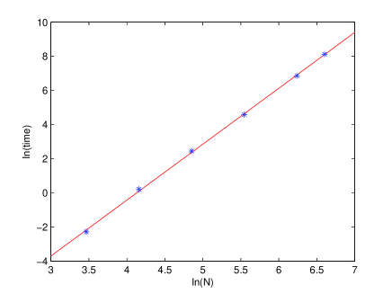
Figure 1: preparation time

In Figure 1, the blue stars are the data and the red line is the linear fitting of the data. Figure 1 shows that the preparation time increases at the rate of $N^{3.3}$ as $N$ increases. It increases significantly when $N$ gets larger.

Fortunately, the preparation step needs to be run only once before the calculation step starts. The calculation step takes about $1.3\times 10^{-6}$ seconds on average, which does not depend on any parameter. This is a quite efficient step, which is very suitable for a large amount of evaluations.

6.2.2 Comparison with other methods

In this subsection, we compare the FFT-based method (FM) with the Ewald method (EM) and the lattice sums (LS). We will apply these three methods to six examples with different $k$’s at the points $P^{3}_{1}$ and $P^{3}_{2}$. Different from the 2D case, the preparation time is no longer too small to be ignored in the 3D case. In Tables 16-21, we list the relative errors and the preparation time (p-time) and calculation times (c-time) in the case when $k=1,5,10,25,50,100$. The parameter $N$ in the FFT-based method is changed when $k$ is different.

Table 16: $k=1$, $N=32$

	$P^{3}_{1}$		$P^{3}_{2}$		p-time(s)
	r-error	c-time(s)	r-error	c-time(s)
EM	$3.60\rm{E}-05$	$1.00\rm{E}-3$	$1.02\rm{E}-06$	$1.00\rm{E}-3$	0
LS	$4.29\rm{E}-02$	$6.90\rm{E}-5$	$2.39\rm{E}-05$	$6.90\rm{E}-5$	13.4
FM	$3.73\rm{E}-04$	$1.30\rm{E}-6$	$6.97\rm{E}-05$	$1.29\rm{E}-6$	0.10

Table 17: $k=5$, $N=64$

	$P^{3}_{1}$		$P^{3}_{2}$		p-time(s)
	r-error	c-time(s)	r-error	c-time(s)
EM	$4.09\rm{E}-05$	$1.40\rm{E}-2$	$3.38\rm{E}-06$	$1.40\rm{E}-2$	0
LS	$2.81\rm{E}-03$	$6.90\rm{E}-5$	$2.99\rm{E}-06$	$6.80\rm{E}-5$	14
FM	$6.44\rm{E}-05$	$1.28\rm{E}-6$	$4.58\rm{E}-06$	$1.29\rm{E}-6$	1.24

Table 18: $k=10$, $N=128$

	$P^{3}_{1}$		$P^{3}_{2}$		p-time(s)
	r-error	c-time(s)	r-error	c-time(s)
EM	$8.01\rm{E}-04$	$5.20\rm{E}-2$	$3.19\rm{E}-05$	$4.90\rm{E}-2$	0
LS	$1.00\rm{E}-04$	$1.80\rm{E}-4$	$1.91\rm{E}-05$	$1.82\rm{E}-4$	34
FM	$4.15\rm{E}-04$	$1.30\rm{E}-6$	$3.76\rm{E}-06$	$1.30\rm{E}-6$	11.42

Table 19: $k=25$, $N=256$

	$P^{3}_{1}$		$P^{3}_{2}$		p-time(s)
	r-error	c-time(s)	r-error	c-time(s)
EM	$2.26\rm{E}-04$	$0.33$	$1.31\rm{E}-05$	$0.32$	0
LS	$2.89\rm{E}-04$	$6.65\rm{E}-4$	$2.34\rm{E}-04$	$6.68\rm{E}-4$	125
FM	$4.99\rm{E}-04$	$1.28\rm{E}-6$	$6.19\rm{E}-06$	$1.30\rm{E}-6$	96.2

Table 20: $k=50$, $N=512$

	$P^{3}_{1}$		$P^{3}_{2}$		p-time(s)
	r-error	c-time(s)	r-error	c-time(s)
EM	$1.75\rm{E}-04$	$1.22$	$5.96\rm{E}-05$	$1.21$	0
LS	$4.15\rm{E}-02$	$2.33\rm{E}-3$	$6.68\rm{E}-04$	$2.34\rm{E}-3$	811
FM	$2.52\rm{E}-04$	$1.31\rm{E}-6$	$1.46\rm{E}-06$	$1.28\rm{E}-6$	940

Table 21: $k=100$, $N=736$

	$P^{3}_{1}$		$P^{3}_{2}$		p-time(s)
	r-error	c-time(s)	r-error	c-time(s)
EM	$2.59\rm{E}-04$	$5.32$	$2.75\rm{E}-06$	$6.44$	0
LS	$7.79\rm{E}-01$	$1.62\rm{E}-3$	$6.23\rm{E}-03$	$1.63\rm{E}-3$	828
FM	$1.31\rm{E}-04$	$1.29\rm{E}-6$	$3.64\rm{E}-06$	$1.30\rm{E}-6$	3322

From the tables above, we see that the Ewald’s method is able to achieve any required accuracy and does not have any preparation time. However, the calculation time taken up by this method grows significantly as $k$ increases. Similar to the 2D case, the lattice sums also suffer from the problems of convergence when $k$ is relatively larger. The calculation time of this method is much less than that of the Ewald method, but still more than that of the FFT-based method. The FFT-based method is the fastest one and works well for all $k$’s with a dependent calculation time. However, when $k$ increases, a larger $N$ is required for the same accuracy, which leads to a significant growth in the preparation time and memory. Thus, when a small number of values or high accuracies are needed, the Ewald’s method is the best choice, while, if a large amount of evaluations is required, the FFT-based method is more competitive.

6.3 Numerical examples for $\mathbb{G}(x)$

In this section, we present some numerical examples for the calculation of $\mathbb{G}(x)$ by Algorithm 4.1. We will present six numerical examples to show the efficiency of this algorithm. The maximum relative error ($\max_{j,l=1,2,3}\frac{|\mathbb{G}_{jl}(x)-\tilde{\mathbb{G}}_{jl}(x)|}{|\mathbb{G}_{jl}(x)|}$), is calculated at each point, and the values for $N=32,64,128,256,512$ are shown in Tables 22-27.

Table 22: $k=1$, $\alpha_{1}=0.1$, $\alpha_{2}=0.2$

	$P^{3}_{1}$	$P^{3}_{2}$	$P^{3}_{3}$	$P^{3}_{4}$
$N=32$	$1.09\rm{E}-02$	$2.65\rm{E}-06$	$3.42\rm{E}-01$	$4.18\rm{E}-04$
$N=64$	$9.00\rm{E}-06$	$6.96\rm{E}-08$	$2.49\rm{E}-04$	$8.82\rm{E}-06$
$N=128$	$2.50\rm{E}-06$	$3.04\rm{E}-10$	$6.99\rm{E}-06$	$1050\rm{E}-08$
$N=256$	$5.61\rm{E}-07$	$1.12\rm{E}-11$	$3.61\rm{E}-07$	$3.55\rm{E}-11$
$N=512$	$4.71\rm{E}-07$	$5.14\rm{E}-12$	$9.90\rm{E}-09$	$1.48\rm{E}-11$

Table 23: $k=5$, $\alpha_{1}=0.1$, $\alpha_{2}=0.2$

	$P^{3}_{1}$	$P^{3}_{2}$	$P^{3}_{3}$	$P^{3}_{4}$
$N=32$	$6.92\rm{E}-03$	$6.25\rm{E}-05$	$4.12\rm{E}-02$	$3.86\rm{E}-04$
$N=64$	$8.84\rm{E}-05$	$2.39\rm{E}-06$	$8.85\rm{E}-05$	$5.56\rm{E}-06$
$N=128$	$2.49\rm{E}-05$	$4.93\rm{E}-07$	$2.42\rm{E}-05$	$1.16\rm{E}-06$
$N=256$	$3.81\rm{E}-06$	$1.71\rm{E}-08$	$3.68\rm{E}-06$	$4.07\rm{E}-08$
$N=512$	$1.26\rm{E}-07$	$6.19\rm{E}-09$	$9.24\rm{E}-08$	$1.44\rm{E}-08$

Table 24: $k=10$, $\alpha_{1}=0.8$, $\alpha_{2}=\sqrt{2}$

	$P^{3}_{1}$	$P^{3}_{2}$	$P^{3}_{3}$	$P^{3}_{4}$
$N=32$	$1.48\rm{E}-01$	$1.00\rm{E}-03$	$1.36\rm{E}-01$	$2.74\rm{E}-03$
$N=64$	$2.12\rm{E}-03$	$4.24\rm{E}-05$	$2.24\rm{E}-03$	$1.31\rm{E}-04$
$N=128$	$4.41\rm{E}-04$	$3.09\rm{E}-06$	$4.56\rm{E}-04$	$1.16\rm{E}-05$
$N=256$	$6.68\rm{E}-05$	$1.48\rm{E}-07$	$6.91\rm{E}-05$	$4.63\rm{E}-07$
$N=512$	$1.53\rm{E}-06$	$4.23\rm{E}-08$	$1.60\rm{E}-06$	$1.59\rm{E}-07$

Table 25: $k=25$, $\alpha_{1}=0.8$, $\alpha_{2}=\sqrt{2}$

	$P^{3}_{1}$	$P^{3}_{2}$	$P^{3}_{3}$	$P^{3}_{4}$
$N=64$	$4.53\rm{E}-02$	$1.51\rm{E}-03$	$4.47\rm{E}-02$	$6.22\rm{E}-03$
$N=128$	$4.62\rm{E}-03$	$6.64\rm{E}-05$	$5.12\rm{E}-03$	$2.54\rm{E}-04$
$N=256$	$6.93\rm{E}-04$	$6.34\rm{E}-06$	$7.70\rm{E}-04$	$2.62\rm{E}-05$
$N=512$	$1.32\rm{E}-05$	$6.67\rm{E}-07$	$1.52\rm{E}-05$	$2.74\rm{E}-06$

Table 26: $k=50$, $\alpha_{1}=\sqrt{3}$, $\alpha_{2}=0.5$

	$P^{3}_{1}$	$P^{3}_{2}$	$P^{3}_{3}$	$P^{3}_{4}$
$N=128$	$3.20\rm{E}-02$	$7.35\rm{E}-04$	$2.78\rm{E}-02$	$1.69\rm{E}-03$
$N=256$	$5.28\rm{E}-03$	$5.93\rm{E}-05$	$4.55\rm{E}-03$	$1.65\rm{E}-04$
$N=512$	$2.69\rm{E}-04$	$6.80\rm{E}-06$	$2.43\rm{E}-04$	$1.21\rm{E}-05$
$N=736$	$1.09\rm{E}-04$	$8.00\rm{E}-07$	$9.37\rm{E}-05$	$1.43\rm{E}-06$

Table 27: $k=100$, $\alpha_{1}=\sqrt{3}$, $\alpha_{2}=0.5$

	$P^{3}_{1}$	$P^{3}_{2}$	$P^{3}_{3}$	$P^{3}_{4}$
$N=256$	$2.00\rm{E}-02$	$1.90\rm{E}-03$	$4.68\rm{E}-02$	$1.46\rm{E}-02$
$N=512$	$2.22\rm{E}-03$	$4.13\rm{E}-05$	$1.54\rm{E}-03$	$4.73\rm{E}-04$
$N=736$	$2.35\rm{E}-04$	$4.69\rm{E}-06$	$5.88\rm{E}-04$	$4.30\rm{E}-05$

From the examples above, similar results can be concluded as those in Subsection 6.2.1. We do not show the preparation and calculation time as they are both about six times longer than those taken by Algorithm 3.1. This implies that our method for the calculation of $\mathbb{G}(x)$ is still highly efficient, especially when a large number of values are needed.

References

• [1] T. Arens, K. Sandfort, S. Schmitt and A. Lechleiter 2013 Analysing Ewald’s method for the evaluation of Green’s functions for periodic media, IMA J. Numer. Anal. 78(3) 405-431.
• [2] G. Beylkin, C. Kurcz and L. Monzón 2008 Fast algorithms for Helmholtz Green’s functions, Proc. R. Soc. A464 3301-3326.
• [3] O.P. Bruno and B. Delourme 2014 Rapidly convergent two-dimensional quasi-periodic Green function throughout the spectrum - including Wood anomalies, J. Comput. Phys. 262 262-290.
• [4] O.P. Bruno and A.G. Fernandez-Lado 2017 Rapidly convergent quasi-periodic Green functions for scattering by arrays of cylinders–including Wood anomalies, Proc. R. Soc. A473, in press.
• [5] F. Capolino, D.R. Wilton, and W.A. JohnsonZ 2002 Efficient computation of the 2-D Green’s function for 1-D periodic structures using the Ewald method, IEEE Trans. Antennas Propagat. 53(4) 2977-2984.
• [6] T.F. Eibert, J.L. Volakis, D.R. Wilton, and D.R. Jackson 1999 Hybrid FE/BI modeling of 3-D doubly periodic structures utilizing triangular prismatic elements and an MPIE formulation accelerated by the Ewald transformation, IEEE Trans. Antennas Propagat. 47 843-850.
• [7] N. Guerin, S. Enoch, and G. Tayeb 2001 Combined method for the computation of the doubly periodic Green’s function, J. Electrom. Waves Appl. 15 205-221.
• [8] T. Hohage 2006 Fast numerical solution of the electromagnetic medium scattering problem and applications to the inverse problem, J. Comput. Phys. 214 224-238.
• [9] R.E. Jorgenson and R. Mittra 1990 Efficient calculation of the free-space periodic Green’s function, IEEE Trans. Antennas Propagat. 38 633-642.
• [10] H. Kurkcu and F. Reitich 2009 Stable and efficient evaluation of periodized Green’s functions for the Helmholtz equation at high frequencies, J. Comput. Phys. 228 75-95.
• [11] A. Kustepeli and A.Q. Martin 2000 On the splitting parameter in the Ewald method, IEEE Microwave Guided Wave Lett. 10 168-170.
• [12] A. Lechleiter and D.L. Nguyen 2012 Spectral volumetric integral equation methods for acoustic medium scattering in 3D waveguide, IMA J. Numer. Anal. 32(3) 813-844.
• [13] F. Lekien and J. Marsden 2005 Tricubic interpolation in three dimensions. Int. J. Numer. Meth. Engng. 63 455-471.
• [14] C.M. Linton 1998 The Green’s function for the two-dimensional Helmholtz equation in periodic domains, J. Eng. Math. 33 377-402.
• [15] C.M. Linton and I. Thompson 2009 One- and two-dimensional lattice sums for the threedimensional Helmholtz equation, J. Comput. Phys. 228 1815-1829.
• [16] C.M. Linton 2010 Lattice Sums for the Helmholtz Equation, SIAM Rev. 52(4) 630-674.
• [17] C.M. Linton 2015 Two-dimensional, phase modulated lattice sums with application to the Helmholtz Green’s function, J. Math. Phys. 56 013505.
• [18] A.W. Mathis and A.F. Peterson 1998 Efficient electromagnetic analysis of a doubly infinite array of rectangular apertures, IEEE Trans. Microwave Theory Tech. 46 46-54.
• [19] A. Moroz 2002 On the computation of the free-space doubly-periodic Green’s function of the threedimensional Helmholtz equation, J. of Electrom. Waves Appl. 16 457-465.
• [20] A. Moroz 2006 Quasi-periodic Green’s functions of the Helmholtz and Laplace equations, J. Phys. A39 11247-11282.
• [21] S. Oroskar, D.R. Jackson, and D.R. Wilton 2006 Efficient computation of the 2D periodic Green’s function using the Ewald method, J. Comput. Phys. 219 899-911.
• [22] N.A. Ozdemir and C. Craeye 2009 Evaluation of the periodic Green’s function near Wood’s anomaly and application to the array scanning method, IEEE Antennas Propag. Soc. Int. Symposium.
• [23] V.G. Papanicolaou 1999 Ewald’s method revisited: Rapidly convergent series representations of certain Green’s functions, J. Comput. Anal. Appl. 1 105-114.
• [24] K. Sandfort, The Factorization Method for Inverse Scattering From Periodic Inhomogeneous Media, PhD Thesis, KIT, KIT Scientific Publishing, 2010, Germany.
• [25] M.G. Silveirinha and C.A. Fernandes 2005 A new acceleration technique with exponential convergence rate to evaluate periodic Green functions, IEEE Trans. Antennas Propagat. 53 347-355.
• [26] I. Stevanovi’c, P. Crespo-Valero, K. Blagovi’c, F. Bongard, and J.R. Mosig 2006 Integral equation analysis of 3-D metallic objects arranged in 2-D lattices using the Ewald transformation, IEEE Trans. Microwave Theory Tech. 54 3688-3697.
• [27] G. Vainikko, Fast solvers of the Lippmann-Schwinger equation, in: Direct and Inverse Problems of Mathematical Physics (eds. R.P. Gilbert, J. Kajiwara and Y. Xu), Kluwer, Dordrecht, The Netherlands, 2000, pp. 423-440.
• [28] G. Valerio, P. Baccarelli, P. Burghignoli, and A. Galli 2007 Comparative analysis of acceleration techniques for 2-D and 3-D Green’s functions in periodic structures along one and two directions, IEEE Trans. Antennas Propagat. 55 1630-1643.
• [29] J.A.C. Weideman 1994 Computation of the complex error function, SIAM. J. Numer Anal 31(5) 1497-1518.
• [30] K. Yasumoto and K. Yoshitomi 1999 Efficient calculation of lattice sums for free-space periodic Green’s function, IEEE Trans. Antennas Propagat. 47 1050-1055.