A Combinatorial Approach to Rauzy-type Dynamics II:
the Labelling Method and a Second Proof
of the KZB Classification Theorem

1 Permutational diagram monoids and groups

The labelling method that we introduce in section 2 is a method to classify Rauzy-type dynamics. In this section we define what we mean by Rauzy-type dynamics.

Let $X_{I}$ be a set of labelled combinatorial objects, with elements labelled from the set $I$. We shall identify it with the set $[n]=\{1,2,\ldots,n\}$ (and use the shortcut $X_{n}\equiv X_{[n]}$). The symmetric group $\mathfrak{S}_{n}$ acts naturally on $X_{n}$, by producing the object with permuted labels.

Vertex-labeled graphs (or digraphs, or hypergraphs) are a typical example. Set partitions are a special case of hypergraphs (all vertices have degree 1). Matchings are a special case of partitions, in which all blocks have size 2. Permutations $\sigma$ are a special case of matchings, in which each block $\{i,j\}$ has $i\in\{1,2,\ldots,n\}$ and $j=\sigma(i)+n\in\{n+1,n+2,\ldots,2n\}$.

We will consider dynamics over spaces of this type, generated by operators of a special form that we now introduce:

Definition 1 (Monoid and group operators).

We say that $A$ is a monoid operator on set $X_{n}$, if, for a map $\alpha:X_{n}\to\mathfrak{S}_{n}$, it consists of the map on $X_{n}$ defined by

$$A(x)=\alpha_{x}x\,,$$ (1)

where the action $\alpha_{x}x$ is in the sense of the symmetric-group action over $X_{n}$. We say that $A$ is a group operator if, furthermore, $\alpha_{A(x)}=\alpha_{x}$.

Said informally, the function $\alpha$ “poses a question” to the structure $x$. The possible answers are different permutations, by which we act on $x$. Note that is all our applications the set $Y_{n}=\{\alpha_{x}|x\in X_{n}\}$ of all possible permutations has a much smaller cardinality than $X_{n}$ and $\mathfrak{S}_{n}$, i.e. very few ‘answers’ are possible. In the Rauzy case, $|X_{n}|=|\mathfrak{S}_{n}|=n!$ while $|Y_{n}|=n$. The asymptotic behaviour is similar ($|X_{n}|$ is at least exponential in $n$, while $|Y_{n}|$ is linear) in all of our applications.

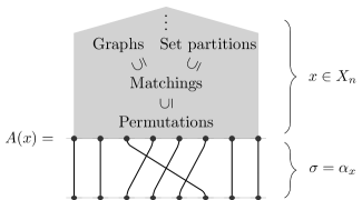
Figure 1: Let $x\in X_{n}$ be a combinatorial structure on $n$ vertices. $A_{x}$ choose a permutation $\sigma$ depending on $x$ and permutes the vertices of $x$ according to it. We represent this symmetric-group action as a diagrammatic action from below.

Clearly we have:

Proposition 2.

Group operators are invertible.

Proof. For a given value of $n$, let $A$ be a group operator on the set $X_{n}$. The property $\alpha_{A(x)}=\alpha_{x}$ implies that, for all $k\in\mathbb{N}$, $A^{k}(x)=(\alpha_{x})^{k}x$. Thus, for all $x$ there exists an integer $d_{A}(x)\in\mathbb{N}^{+}$ such that $A^{d_{A}(x)}(x)=x$. More precisely, $d_{A}(x)$ is (a divisor of) the l.c.m. of the cycle-lengths of $\alpha_{x}$. Call $d_{A}=\operatorname{lcm}_{x\in X_{n}}d_{A}(x)$ (i.e., more shortly, the l.c.m. over $y\in Y_{n}$ of the cycle-lengths of $\alpha_{y}$). Then $d_{A}$ is a finite integer, and we can pose $A^{-1}=A^{d_{A}-1}$. The reasonings above show that $A$ is a bijection on $X_{n}$, and $A^{-1}$ is its inverse. $\square$

Definition 3 (monoid and group dynamics).

We call a monoid dynamics the datum of a family of spaces $\{X_{n}\}_{n\in\mathbb{N}}$ as above, and a finite collection $\mathcal{A}=\{A_{i}\}$ of monoid operators. We call a group dynamics the analogous structure, in which all $A_{i}$’s are group operators.

For a monoid dynamics on the datum $S_{n}=(X_{n},\mathcal{A})$, we say that $x,x^{\prime}\in X_{n}$ are strongly connected, $x\sim x^{\prime}$, if there exist words $w,w^{\prime}\in\mathcal{A}^{*}$ such that $wx=x^{\prime}$ and $w^{\prime}x^{\prime}=x$.

For a group dynamics on the datum $S_{n}=(X_{n},\mathcal{A})$, we say that $x,x^{\prime}\in X_{n}$ are connected, $x\sim x^{\prime}$, if there exists a word $w\in\mathcal{A}^{*}$ such that $wx=x^{\prime}$.

Here the action $wx$ is in the sense of monoid action. Being connected is clearly an equivalence relation, and coincides with the relation of being graph-connected on the Cayley Graph associated to the dynamics, i.e. the digraph with vertices in $X_{n}$, and edges $x\longleftrightarrow_{i}x^{\prime}$ if $A_{i}^{\pm 1}x=x^{\prime}$. An analogous statement holds for strong-connectivity, and the associated Cayley Digraph.

We call such dynamics Rauzy-type dynamics since the original Rauzy dynamics that inspired this definition is also of this type.

Definition 4 (classes of configurations).

Given a dynamics as above, and $x\in X_{n}$, we define $C(x)\subseteq X_{n}$, the class of $x$, as the set of configurations connected to $x$, $C(x)=\{x^{\prime}\,:\,x\sim x^{\prime}\}$.

We will call those classes the Rauzy classes of the dynamics.

Definition 5 (Invariant of classes).

Given a dynamics as above, we say that $f:X_{n}\to G_{n}$ is an invariant of the dynamics if $f(x)=f(x^{\prime})$ for every pair $(x,x^{\prime})$ of connected combinatorial structures.

Thus given a dynamics $(X_{n},\mathcal{A})$ our goal is to find a family of invariant $(f_{i})$ such that two combinatorial structures are in the same Rauzy class if and only if they have the same invariants.

2 Definition of the Rauzy dynamics

We will now apply the labelling method defined in the previous section to give an original proof of the classification of the Rauzy dynamics. Other proofs have been achieved in [Boi12] (Boissy uses the classification proof for the extended Rauzy dynamics appearing in [KZ03]) using geometric methods and in [Fic16] and [DS17] using combinatorial methods.

The extended Rauzy classes (classified in [KZ03]) are of interest in the translation surface field as they are in one-to-one correspondance with the connected components of the strata of the moduli space of abelian differentials (see [Vee82]). As for the non-extended Rauzy classes, they are in one-to-one correspondance with the connected components of the strata of the moduli space of abelian differentials with a marked zero as shown in [Boi12].

2.1 The Rauzy dynamics

$$\begin{array}[]{cc}m=\big{(}(16)(24)(37)(58)\big{)}\in\mathcal{M}_{8}&\sigma=[41583627]\in\mathfrak{S}_{8}\subseteq\mathcal{M}_{16}\\ &\textrm{matching diagram representation}\\ \raisebox{7.0pt}{ \begin{picture}(10.0,4.0)(0.0,-1.0)\put(0.0,0.2){\includegraphics[scale={2.5}]{FigFol/Figure1_fig_exMatch_16243758_.pdf}} \put(0.5,-0.25){\rotatebox{30.0}{\makebox[0.0pt][r]{\scriptsize{$\bm{1}$}}}} \put(6.8,-0.25){\rotatebox{30.0}{\makebox[0.0pt][r]{\scriptsize{$m(1)=\bm{6}$}}}} \end{picture} }&\rule{0.0pt}{72.0pt}\raisebox{7.0pt}{ \begin{picture}(20.0,4.0)(0.0,-1.0)\put(0.0,0.0){\includegraphics[scale={2.5}]{FigFol/Figure1_fig_exPerm_41583627_match.pdf}} \put(0.5,-0.25){\rotatebox{30.0}{\makebox[0.0pt][r]{\scriptsize{$\bm{1}$}}}} \put(14.5,-0.25){\rotatebox{30.0}{\makebox[0.0pt][r]{\scriptsize{$n+\sigma(1)=\bm{12}$}}}} \end{picture} }\\ \rule{0.0pt}{22.0pt}\sigma=[41583627]\in\mathfrak{S}_{8}&\sigma=[41583627]\in\mathfrak{S}_{8}\\ \textrm{diagram representation}&\textrm{matrix representation}\\ \raisebox{12.5pt}{ \begin{picture}(11.0,3.0)\put(0.0,0.0){\includegraphics[scale={2.5}]{FigFol/Figure1_fig_exPerm_41583627_.pdf}} \put(0.9,-0.15){\rotatebox{-30.0}{\scriptsize{$\bm{1}$}}} \put(3.6,5.4){\rotatebox{-30.0}{\makebox[0.0pt][c]{\scriptsize{$\sigma(1)=\bm{4}$}}}} \end{picture} }&\rule{0.0pt}{90.0pt}\raisebox{0.0pt}{ \begin{picture}(8.0,8.0)\put(0.0,0.0){\includegraphics[scale={1}]{FigFol/Figure1_fig_matr_exPerm_41583627_.pdf}} \put(0.4,-0.6){\scriptsize{$\bm{1}$}} \put(-0.3,3.4){\makebox[0.0pt][r]{\scriptsize{$\sigma(1)=\bm{4}$}}} \end{picture} }\end{array}$$

Figure 2: Diagram representations of matchings and permutations, and matrix representation of permutations.

Let $\mathfrak{S}_{n}$ denote the set of permutations of size $n$, and $\mathfrak{M}_{n}$ the set of matchings over $[2n]$, thus with $n$ arcs. Let us call $\omega$ the permutation $\omega(i)=n+1-i$.

A permutation $\sigma\in\mathfrak{S}_{n}$ can be seen as a special case of a matching over $[2n]$, in which the first $n$ elements are paired to the last $n$ ones, i.e. the matching $m_{\sigma}\in\mathfrak{M}_{n}$ associated to $\sigma$ is $m_{\sigma}=\{(i,\sigma(i)+n)\,|\,i\in[n]\}.$

We say that $\sigma\in\mathfrak{S}_{n}$ is irreducible if $\omega\sigma$ doesn’t leave stable any interval $\{1,\ldots,k\}$, for $1\leq k<n$, i.e. if $\{\sigma(1),\ldots,\sigma(k)\}\neq\{n-k+1,\ldots,n\}$ for any $k=1,\ldots,n-1$. We also say that $m\in\mathfrak{M}_{n}$ is irreducible if it does not match an interval $\{1,\ldots,k\}$ to an interval $\{2n-k+1,\ldots,2n\}$. Let us call $\mathfrak{S}^{\rm irr}_{n}$ and $\mathfrak{M}^{\rm irr}_{n}$ the corresponding sets of irreducible configurations.

We represent matchings over $[2n]$ as arcs in the upper half plane, connecting pairwise $2n$ points on the real line (see figure 2, top left). Permutations, being a special case of matching, can also be represented in this way (see figure 2, top right), however, in order to save space and improve readibility, we rather represent them as arcs in a horizontal strip, connecting $n$ points at the bottom boundary to $n$ points on the top boundary (as in Figure 2, bottom left). Both sets of points are indicised from left to right. We use the name of diagram representation for such representations.

We will also often represent configurations as grids filled with one bullet per row and per column (and call this matrix representation of a permutation). We choose here to conform to the customary notation in the field of Permutation Patterns, by adopting the algebraically weird notation, of putting a bullet at the Cartesian coordinate $(i,j)$ if $\sigma(i)=j$, so that the identity is a grid filled with bullets on the anti-diagonal, instead that on the diagonal. An example is given in figure 2, bottom right.

Let us define a special set of permutations (in cycle notation)

$$\gamma_{L,n}(i) =(i-1\;i-2\;\cdots\;1)(i)(i+1)\cdots(n)\,;$$ (2a)

$$\gamma_{R,n}(i) =(1)(2)\cdots(i)(i+1\;i+2\;\cdots\;n)\,;$$ (2b)

i.e., in a picture in which the action is diagrammatic, and acting on structures $x\in X_{n}$ from below,

$$\gamma_{L,n}(i): \scriptstyle{1} \scriptstyle{i} \scriptstyle{n} \gamma_{R,n}(i): \scriptstyle{1} \scriptstyle{i} \scriptstyle{n}$$

Of course, $\omega\gamma_{L,n}(i)\omega=\gamma_{R,n}(n+1-i)$.

$$L\;\Big{(}\;\raisebox{-15.0pt}{\reflectbox{\includegraphics[scale={1.5}]{FigFol/Figure1_fig_Mlr2bul.pdf}}}\;\Big{)} =\raisebox{-15.0pt}{\reflectbox{\includegraphics[scale={1.5}]{FigFol/Figure1_fig_Mlr1bul.pdf}}} R\;\Big{(}\;\raisebox{-15.0pt}{\includegraphics[scale={1.5}]{FigFol/Figure1_fig_Mlr2bul.pdf}}\;\Big{)} =\raisebox{-15.0pt}{\includegraphics[scale={1.5}]{FigFol/Figure1_fig_Mlr1bul.pdf}}$$

$$L\;\Big{(}\;\raisebox{14.2pt}{\includegraphics[scale={1.75},angle={180}]{FigFol/Figure1_fig_PPlr1_simp.pdf}}\;\Big{)} =\raisebox{27.2pt}{\includegraphics[scale={1.75},angle={180}]{FigFol/Figure1_fig_PPlr2_simp.pdf}}\rule{0.0pt}{38.0pt} R\;\Big{(}\;\raisebox{-9.0pt}{\includegraphics[scale={1.75}]{FigFol/Figure1_fig_PPlr1_simp.pdf}}\;\Big{)} =\raisebox{-24.0pt}{\includegraphics[scale={1.75}]{FigFol/Figure1_fig_PPlr2_simp.pdf}}$$

Figure 3: Our two main examples of dynamics, in diagram representation. Top: the $\mathcal{M}_{n}$ case. top: the $\mathcal{S}_{n}$ case.

$$L\;\left(\;\raisebox{-25.0pt}{\includegraphics[scale={.499}]{FigFol/Figure1_fig_matrix_dyna_1.pdf}}\;\right) =\raisebox{-25.0pt}{\includegraphics[scale={.499}]{FigFol/Figure1_fig_matrix_dyna_2_L.pdf}}\rule{0.0pt}{38.0pt} R\;\left(\;\raisebox{-25.0pt}{\includegraphics[scale={.499}]{FigFol/Figure1_fig_matrix_dyna_1.pdf}}\;\right) =\raisebox{-25.0pt}{\includegraphics[scale={.499}]{FigFol/Figure1_fig_matrix_dyna_3_R.pdf}}$$

Figure 4: The Rauzy dynamics concerning permutations, in matrix representation.

The Rauzy dynamics $\mathcal{S}_{n}$ that we study in this article is defined as a special case of the $\mathcal{M}_{n}$ dynamics:

$\mathcal{M}_{n}$ :

The space of configuration is $\mathfrak{M}^{\rm irr}_{n}$, irreducible $n$-arc matchings. There are two generators, $L$ and $R$, with $\alpha_{L}(m)=\gamma_{L,2n}(m(1))$ and $\alpha_{R}(m)=\gamma_{R,2n}(m(2n))$ ($\alpha$ is as in Definition 1). See Figure 3, top.

$\mathcal{M}_{n}$$\mathcal{S}_{n}$ :

The space of configuration is $\mathfrak{S}^{\rm irr}_{n}$, irreducible permutations of size $n$. Again, there are two generators, $L$ and $R$. If permutations are seen as matchings such that indices in $\{1,\ldots,n\}$ are paired to indices in $\{n+1,\ldots,2n\}$, the dynamics coincide with the one given above. See Figure 3, bottom.

The motivation for restricting to irreducible permutations and matchings shall be clear at this point: a non-irreducible permutation is a grid with a non-trivial block-decomposition. The operators $L$ and $R$ only act on the first block (say, of size $k$), so that the study of the dynamics trivially reduces to the study of the $\mathcal{S}_{k}$ dynamics on these blocks (see figure 5).

Figure 5: Left: A reducible permutation in matrix representation; the $\mathcal{S}$ dynamic acts on the first block with $L$ and $R$. Right: A reducible permutation in diagram representation; the $\mathcal{S}$ dynamics acts on the gray part with $L$ and $R$, while leaving the blue part unchanged.

This simple observation, however, comes with a disclaimer: To apply the labelling method we must guarantee that the outcome of our manipulations on irreducible configurations is still irreducible during the induction steps in the classification theorem. We explain this problem in the overview section. (The solution will be to choose normal forms that take this problem into account).

2.2 Definition of the invariants

The main purpose of this article, is to characterise the classes appearing in the so called Rauzy dynamics $\mathcal{S}_{n}$ using the labelling method. This gives a third combinatorial proof of this result, the two preceding ones can be found in [DS17] and [Fic16].

In this section we recall the definition of the invariants, the proof of their invariance can be found in [DS17].

2.2.1 Cycle invariant

Let $\sigma$ be a permutation, identified with its diagram. An edge of $\sigma$ is a pair $(i^{-},j^{+})$, for $j=\sigma(i)$, where $-$ and $+$ denote positioning at the bottom and top boundary of the diagram. Perform the following manipulations on the diagram: (1) replace each edge with a pair of crossing edges; more precisely, replace each edge endpoint, say $i^{-}$, by a black and a white endpoint, $i_{b}^{-}$ and $i_{w}^{-}$ (the black on the left), then introduce the edges $(i_{b}^{-},j_{w}^{+})$ and $(i_{w}^{-},j_{b}^{+})$. (2) connect by an arc the points $i_{w}^{\pm}$ and $(i+1)_{b}^{\pm}$, for $i=1,\ldots,n-1$, both on the bottom and the top of the diagram; (3) connect by an arc the top-right and bottom-left endpoints, $n_{w}^{+}$ and $1_{b}^{-}$. Call this arc the “$-1$ mark”.

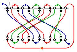
Figure 6: Left: an irreducible permutation, $\sigma=[\,451263\,]$. Right: the construction of the cycle structure. Different cycles are in different colour. The length of a cycle or path, defined as the number of top (or bottom) arcs, is thus 2 for red and violet, and 1 for blue. The green arrows are the endpoints of the rank path, which is in blue. As a result, in this example $\lambda(\sigma)=(2,2)$ (for the cycles of color red and violet), $r(\sigma)=1$ (corresponding to the rank path of color blue), and $\ell(\sigma)=2$.

The resulting structure is composed of a number of closed cycles, and one open path connecting the top-left and bottom-right endpoints, that we call the rank path. If it is a cycle that goes through the $-1$ mark (and not the rank path), we call it the principal cycle. Define the length of an (open or closed) path as the number of top (or bottom) arcs (connecting a white endpoint to a black endpoint) in the path. These numbers are always positive integers (for $n>1$ and irreducible permutations). The length $r$ of the rank path will be called the rank of $\sigma$, and $\lambda=\{\lambda_{i}\}$, the collection of lengths of the cycles, will be called the cycle structure of $\sigma$. Define $\ell(\sigma)$ as the number of cycles in $\sigma$ (this does not include the rank). See Figure 6, for an example.

Note that this quantity does not coincide with the ordinary path-length of the corresponding paths. The path-length of a cycle of length $k$ is $2k$, unless it goes through the $-1$ mark, in which case it is $2k+1$. Analogously, if the rank is $r$, the path-length of the rank path is $2r+1$, unless it goes through the $-1$ mark, in which case it is $2r+2$. (This somewhat justifies the name of “$-1$ mark” for the corresponding arc in the construction of the cycle invariant.)

In the interpretation within the geometry of translation surfaces, the cycle invariant is exactly the collection of conical singularities in the surface (we have a singularity of $2k\pi$ on the surface, for every cycle of length $\lambda_{i}=k$ in the cycle invariant, and the rank corresponds to the ‘marked singularity’ of [Boi12], see article [DS17]).

It is easily seen that

$$r+\sum_{i}\lambda_{i}=n-1\,,$$ (3)

this formula is called the dimension formula. Moreover, in the list $\{r,\lambda_{1},\ldots,\lambda_{\ell}\}$, there is an even number of even entries. This is part of theorem 7 stated next section and proven during the induction step.

We have

Proposition 6.

The pair $(\lambda,r)$ is invariant in the $\mathcal{S}$ dynamics.

For a proof, see [DS17] section 3.1.

We have also shown in [DS17] appendix B that cycles of length 1 have an especially simple behaviour and can thus be omitted from the classification theorem. Thus all the classes we consider in this article have a cycle invariant $\lambda$ with no parts of length 1.

2.2.2 Sign invariant

For $\sigma$ a permutation, let $[n]$ be identified to the set of edges (e.g., by labeling the edges w.r.t. the bottom endpoints, left to right). For $I\subseteq[n]$ a set of edges, define $\chi(I)$ as the number of pairs $\{i^{\prime},i^{\prime\prime}\}\subseteq I$ of non-crossing edges. Call

$$\overline{A}(\sigma):=\sum_{I\subseteq[n]}(-1)^{|I|+\chi(I)}$$ (4)

the Arf invariant of $\sigma$ (see Figure 7 for an example). Call $s(\sigma)=\mathrm{Sign}(\overline{A}(\sigma))\in\{-1,0,+1\}$ the sign of $\sigma$.

Both the quantity $\overline{A}(\cdot)$ and $s(\cdot)$ are invariant for the dynamics $\mathcal{S}$. The proof can be found in [DS17] section 4.2. However, in order to illustrate how to automatically compute the arf identities, the proof will be given once more in equation (12).

There exists an important relationship between the arf invariant and the cycle invariant that we describe below. The proof of this theorem will be done during the induction (see the proof overview section for more details).

Theorem 7.

Let $\sigma$ be a permutation with cycle invariant $(\lambda,r)$ and let $\ell$ be the number of cycles (not including the rank) of $\sigma$ i.e. $\ell=|\lambda|$.

• The list $\lambda\bigcup\{r\}$ has an even number of even parts.

• $\overline{A}(\sigma)=\begin{cases}\pm 2^{\frac{n+\ell}{2}}&\text{ if there are no even parts in the list $\lambda\bigcup\{r\}$}\\ 0&\text{ otherwise.}\end{cases}$

as a consequence we have:

Proposition 8.

The sign of $\sigma$ can be written as $s(\sigma)=2^{-\frac{n+\ell}{2}}\overline{A}(\sigma)$, where $\ell$ is the number of cycles of $\sigma$.

$$\begin{array}[]{cp{4mm}c}\includegraphics[scale={4}]{FigFol/Figure1_fig_PE_arfEx1.pdf}&&\includegraphics[scale={4}]{FigFol/Figure1_fig_PE_arfEx2.pdf}\end{array}$$

Figure 7: Left: an example of permutation, $\sigma=[\,251478396\,]$. Right: an example of subset $I=\{1,2,6,8,9\}$ (labels are for the bottom endpoints, edges in $I$ are in blue). There are two crossings, out of the maximal number $\binom{|I|}{2}=10$, thus $\chi_{I}=8$ in this case, and this set contributes $(-1)^{|I|+\chi_{I}}=(-1)^{5+8}=-1$ to $A(\sigma)$.

2.3 Exceptional classes

the invariants described above allow to characterise all classes for the dynamics on irreducible configurations, with two exceptions. These two exceptional classes are called $\mathrm{Id}_{n}$ and ${\mathrm{Id}}^{\prime}_{n}$.

$\mathrm{Id}_{n}$ is called the ‘hyperelliptic class’, because the Riemann surface associated to $\mathrm{Id}_{n}$ is hyperelliptic. Similarly $\mathrm{Id}^{\prime}_{n}$ is often referred to as the ‘hyperelliptic class’ with a marked point).

Those two classes were studied in details in Appendix C of [DS17]. In this article, and as outlined in the labelling method section, we will need to certify that the reduced permutations $y_{1}$ and $y_{2}$ we obtain from $(x^{\prime}_{1},c_{1})$ and $(x^{\prime}_{2},c_{2})$ do not fall into exceptional classes. This will not be very difficult but we will need a short lemma that we included into appendix A. Moreover, to make sense of this lemma we reproduce in this appendix a few results of the appendix C.1 of the paper [DS17].

$$\begin{array}[]{|c|c|c|}\cline{2-3}\cr\lx@intercol\hfil\hfil\lx@intercol\vrule\lx@intercol&\textrm{$n$ even}&\textrm{$n$ odd}\\ \hline\cr(\lambda,r)\text{ of }\mathrm{Id}_{n}&(\varnothing,n-1)&\raisebox{-5.0pt}{\rule{0.0pt}{15.0pt}}(\{\frac{n-1}{2}\},\frac{n-1}{2})\\ \hline\cr(\lambda,r)\text{ of }{\mathrm{Id}}^{\prime}_{n}&\raisebox{-5.0pt}{\rule{0.0pt}{15.0pt}}(\{\frac{n-2}{2},\frac{n-2}{2}\},1)&(\{n-2\},1)\\ \hline\cr\end{array}$$

$$\begin{array}[]{|c|cccccccc|}\cline{2-9}\cr\lx@intercol\hfil n\mod 8\hfil\lx@intercol\vrule\lx@intercol&0&1&2&3&4&5&6&7\\ \hline\cr s\text{ of }\mathrm{Id}_{n}&+&0&-&-&-&0&+&+\\ \hline\cr s\text{ of }{\mathrm{Id}}^{\prime}_{n}&+&+&0&-&-&-&0&+\\ \hline\cr\end{array}$$

Table 1: Cycle, rank and sign invariants of the exceptional classes. The sign $s\in\{-1,0,+1\}$ is shortened into $\{-,0,+\}$.

The cycle and sign invariants of these classes depend from their size mod 4, and are described in Table 1.

2.4 The classification theorems

For the case of the $\mathcal{S}$ dynamics, we have a classification involving the cycle structure $\lambda(\sigma)$, the rank $r(\sigma)$ and sign $s(\sigma)$ described in Section 2.2

Theorem 9.

Besides the exceptional classes $\mathrm{Id}$ and ${\mathrm{Id}}^{\prime}$, which have cycle and sign invariants described in Table 1, the number of classes with cycle invariant $(\lambda,r)$ (no $\lambda_{i}=1$) depends on the number of even elements in the list $\{\lambda_{i}\}\cup\{r\}$, and is, for $n\geq 9$,

zero,

if there is an odd number of even elements;

zero,one,

if there is a positive even number of even elements; the class then has sign 0.

zero,two,

if there are no even elements at all. The two classes then have non-zero opposite sign invariant.

For $n\leq 8$ the number of classes with given cycle invariant may be smaller than the one given above, and the list in Table 2 gives a complete account.

As a consequence, two permutations $\sigma$ and $\sigma^{\prime}$, not of $\mathrm{Id}$ or ${\mathrm{Id}}^{\prime}$ type, are in the same class iff they have the same cycle and sign invariant.

$$\begin{array}[]{r||c|c|cccccc}n&\mathrm{Id}&\mathrm{Id}^{\prime}&\lx@intercol\hfil\textrm{non-exceptional classes}\hfil\lx@intercol\\ \hline\cr 4&\varnothing|3-&\\ 5&2|2&3|1-\\ 6&\varnothing|5+&22|1&\varnothing|5-\\ 7&3|3+&5|1+&2|4&4|2&3|3-&5|1-\\ 8&\varnothing|7+&33|1+&22|3&32|2&42|1&33|1-&\varnothing|7+&\varnothing|7-\end{array}$$

Table 2: List of invariants $(\lambda,r,s)$ for $n\leq 8$, for which the corresponding class in the $\mathcal{S}_{n}$ dynamics exists. We shorten $s$ to $\{-,+\}$ if valued $\{-1,+1\}$, and omit it if valued 0.

The original theorem from Kontsevich and Zorich [KZ03] classifies the extended Rauzy dynamics $\mathcal{S}^{\rm ex}$, however we have shown in section 6.5 of [DS17] that this theorem is a simple corollary of Theorem 9.

3 The sign invariant

3.1 Arf functions for permutations

For $\sigma$ a permutation in $\mathfrak{S}_{n}$, let

$$\chi(\sigma)=\#\{1\leq i<j\leq n\;|\;\sigma(i)<\sigma(j)\}$$ (5)

i.e. $\chi(\sigma)$ is the number of pairs of non-crossing edges in the diagram representation of $\sigma$.

Let $E=E(\sigma)$ be the subset of $n$ edges in $\mathcal{K}_{n,n}$ described by $\sigma$. For any $I\subseteq E$ of cardinality $k$, the permutation $\sigma|_{I}\in\mathfrak{S}_{k}$ is defined in the obvious way, as the one associated to the subgraph of $\mathcal{K}_{n,n}$ with edge-set $I$, with singletons dropped out, and the inherited total ordering of the two vertex-sets.

Define the two functions

$$A(\sigma) :=\sum_{I\subseteq E(\sigma)}(-1)^{\chi(\sigma|_{I})}\,; \overline{A}(\sigma) :=\sum_{I\subseteq E(\sigma)}(-1)^{|I|+\chi(\sigma|_{I})}\,.$$ (6)

When $\sigma$ is understood, we will just write $\chi_{I}$ for $\chi(\sigma|_{I})$. The quantity $A$ is accessory in the forthcoming analysis, while the crucial fact for our purpose is that the quantity $\overline{A}$ is invariant in the $\mathcal{S}_{n}$ dynamics.

In the following section, we define a technique to demonstrate identities of the arf invariant involving differents configurations.

3.2 Automatic proofs of Arf identitites

We will not try to evaluate Arf functions of large configurations starting from scratch. We will rather compare the Arf functions of two (or more) configurations, which differ by a finite number of edges, and establish linear relations among their Arf functions. The method we develop here, gives an algorithm to find and check Arf identities.

In order to have the appropriate terminology for expressing this strategy, let us define the following: Given a permutation $\sigma$ define $\sigma_{k,\ell}$ to be a permutation with $k$ marks on its bottom line and $\ell$ marks on its top line. The marks are all at distinct positions and do not touch the corners of the permutation. These marks break the bottom (respectively top) line into $k+1$ open interval $P_{-,1},\ldots,P_{-,k+1}$ (respectively $\ell+1$ open interval $P_{+,1},\ldots,P_{+,\ell+1}$).

For example if $k=1,\ell=3$:

$$\put(50.0,-30.0){$P_{-,1}$}\put(100.0,-30.0){$P_{-,2}$}\put(26.0,25.0){$P_{+,1}$}\put(60.0,25.0){$P_{+,2}$}\put(90.0,25.0){$P_{+,3}$}\put(125.0,25.0){$P_{+,4}$}\sigma_{k,\ell}=\raisebox{-20.0pt}{\includegraphics[scale={2.5}]{P05_Arf/figure/fig_arf_ex1.pdf}}$$

Let $\sigma_{k,\ell,E^{\prime}}$ be the permutation obtained by adding a set of edges $E^{\prime}$ on the marks of permutation $\sigma_{k,\ell}$ with the following convention: an edge $e\in E^{\prime}$ is a pair $(i.x,j.y)$. The edge connects the $i$th bottom mark and the $j$th top mark, and it is ordered as the $x$th edge within the bottom mark and the $y$th edge within the top mark. Note that if $i=0$ of $i=k+1$ (likewise of $j$) this implies that the edge is connected to a corner of the permutation.

For example if $k=1,\ell=3$ and $E^{\prime}=\{(0.1,2.2),(1.1,3.1),(1.2,1.1),(1.3,2.1),(2,1.2)\}$:

$$\put(60.0,-30.0){$P_{-,1}$}\put(110.0,-30.0){$P_{-,2}$}\put(36.0,25.0){$P_{+,1}$}\put(70.0,25.0){$P_{+,2}$}\put(105.0,25.0){$P_{+,3}$}\put(135.0,25.0){$P_{+,4}$}\sigma_{k,\ell,E^{\prime}}=\raisebox{-20.0pt}{\includegraphics[scale={2.5}]{P05_Arf/figure/fig_arf_ex2.pdf}}$$

We will define an algorithm that allows one to check if, for all $\sigma$, we have $\sum^{n}_{i=1}K_{i}\overline{A}(\sigma_{k,\ell,E^{i}})=0$ or $\sum^{n}_{i=1}K_{i}A(\sigma_{k,\ell,E^{i}})=0$ for some $k,\ell,(E^{i})_{i},(K_{i})_{i},n.$

Definition 10.

Let $\sigma_{k,\ell,E^{\prime}}$, $P_{-,1},\ldots,P_{-,k+1}$ and $P_{+,1},\ldots,P_{+,\ell+1}$ be as defined above. Then define the $m\times(k+1)(\ell+1)$ matrix valued in ${\mathrm{GF}}_{2}$

$$Q_{e,ij}:=\left\{\begin{array}[]{ll}1&\textrm{edge $e\in E^{\prime}$ does not cross the segment connecting $P_{-,i}$ to $P_{+,j}$,}\\ 0&\textrm{otherwise.}\end{array}\right.$$ (7)

For $v\in{\mathrm{GF}}_{2}^{(k+1)(\ell+1)}$, let $|v|$ be the number of entries equal to $1$. Similarly, identify $v$ with the corresponding subset of $[(k+1)(\ell+1)]$. Given such a construction, introduce the following functions on $({\mathrm{GF}}_{2})^{(k+1)(\ell+1)}$

$$A_{k,\ell,E^{\prime}}(v) :=\sum_{u\in({\mathrm{GF}}_{2})^{E^{\prime}}}(-1)^{\chi_{u}+(u,Qv)}\,; \overline{A}_{k,\ell,E^{\prime}}(v) :=\sum_{u\in({\mathrm{GF}}_{2})^{E^{\prime}}}(-1)^{|u|+\chi_{u}+(u,Qv)}\,.$$ (8)

The construction is illustrated in Figure 8.

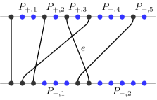
Figure 8: The permutation $\sigma_{1,4,\{(0.1,0.1),(0.2,3.1),(0.3,1.1),(1.1,4.1),(1.2,2.1)\}}$. We cannot show the full matrix $Q$ for such a big example, but we can give one row, for the edge which has the label $e$ in the drawing. The row $Q_{e}$ reads $(Q_{e})_{11,12,\ldots,15,21,\ldots,25}=(1,1,0,0,0,\,0,0,1,1,1)$.

Let us comment on the reasons for introducing such a definition. The quantities $A_{k,\ell,E^{\prime}}(v)$ (respectively $\overline{A}_{k,\ell,E^{\prime}}(v)$) do not depend on $\sigma$ and allows to sum together many contributions to the function $A(\sigma_{k,\ell,E^{\prime}})$. Our goal is to have $E^{\prime}$ of fixed size, while $E$ (the edge set of $\sigma$) is arbitrary and of unbounded size, so that the verification of our properties, as it is confined to the matrix $Q$, involves a finite data structure. Thus the algorithm will be exponential in $|E^{\prime}|$ which will not be a problem for small sizes.

Indeed, let us split in the natural way the sum over subsets $I$ of $E\bigcup E^{\prime}$ the edge set of $\sigma_{k,\ell,E^{\prime}}$ namely

$$\sum_{I_{0}\subseteq E\bigcup E^{\prime}}f(I_{0})=\sum_{I\subseteq E}\sum_{I^{\prime}\subseteq E^{\prime}}f(I\cup I^{\prime})$$

For $I$ and $J$ two disjoint sets of edges, call $\chi_{I,J}$ the number of pairs $(i,j)\in I\times J$ which do not cross. Then clearly

$$\chi_{I\cup J}=\chi_{I}+\chi_{J}+\chi_{I,J}$$

Now let $u(I^{\prime})\in\{0,1\}^{E^{\prime}}$ be the vector with entries $u_{e}=1$ if $e\in I^{\prime}$ and $0$ otherwise. Let $m(I)=\{m_{ij}(I)\}$ be the $(k+1)\times(\ell+1)$ matrix describing the number of edges connecting the intervals $P_{-,i}$ to $P_{+,j}$ in $\sigma$, and let $v(I)=\{v_{ij}(I)\}$, $v_{ij}\in\{0,1\}$ be the parities of the $m_{ij}$’s. Call $I_{ij}$ the restriction of $I$ to edges connecting $P_{-,i}$ and $P_{+,j}$. Clearly,

$$\chi_{I^{\prime},I}=\sum_{ij}\chi_{I^{\prime},I_{ij}}=\sum_{e,ij}u_{e}Q_{e,ij}m_{ij}=(u(I^{\prime}),Qm(I)),$$

which has the same parity as the analogous expression with $v$’s instead of $m$’s. I.e. we have

$$(-1)^{\chi_{I^{\prime},I}}=(-1)^{(u(I^{\prime}),Qv(I))}.$$

Now, while the $m$’s are in $\mathbb{N}$, the vector $v$ is in a linear space of finite cardinality, which is crucial for allowing a finite analysis of our expressions.

As a consequence,

$$A(\sigma_{k,\ell,E^{i}}) =\sum_{I\subseteq E}(-1)^{\chi_{I}}A_{k,\ell,E^{\prime}}(v(I))\,;$$ (9)

$$\overline{A}(\sigma_{k,\ell,E^{i}}) =\sum_{I\subseteq E}(-1)^{|I|+\chi_{I}}\overline{A}_{k,\ell,E^{\prime}}(v(I))\,.$$ (10)

Thus we have the following proposition:

Theorem 11.

Let $k,\ell\in\mathbb{N}$ and let $(E^{i})_{1\leq i\leq n}$ be a family of edge set. Then the two following statements are equivalent:

1. For all $v\in GF_{2}^{(k+1)(\ell+1)},$ we have $\sum_{i=1}^{n}K_{i}A_{k,\ell,E^{i}}(v)=0$.

2. for all $\sigma,$ we have $\sum_{i=1}^{n}K_{i}A(\sigma_{k,\ell,E^{i}})=0.$

The same statement holds for $\overline{A}$.

Proof.  Statement 1 implies 2 due to equation (9).
Let us show the converse: If $\sigma$ has no edge then $\sum_{i=1}^{n}K_{i}A(\sigma_{k,\ell,E^{i}})=0$ is equivalent to $\sum_{i=1}^{n}K_{i}A_{k,\ell,E^{i}}(v)=0$ with $v$ being the zero vector of $(GF_{2})^{(k+1)(\ell+1)}$.

Then we choose the family of permutations $(\sigma^{a,b})_{a,b}$ with exactly one edge connecting $P_{-,a}$ to $P_{+,b}$. Then if we define $v_{a,b}$ to be the vector $(GF_{2})^{(k+1)(\ell+1)}$ with exactly one 1 at position $ab$ we have

$$\sum_{i=1}^{n}K_{i}A(\sigma^{a,b}_{k,\ell,E^{i}})=0$$

$$\iff \sum_{i=1}^{n}K_{i}(A_{k,\ell,E^{i}}(0)+A_{k,\ell,E^{i}}(v_{a,b}))=0$$

$$\iff \sum_{i=1}^{n}K_{i}A_{k,\ell,E^{i}}(v_{a,b})=0$$

in the last line we have used that $\sum_{i=1}^{n}K_{i}A_{k,\ell,E^{i}}(0)=0$.

Thus inductively we show that $\sum_{i=1}^{n}K_{i}A_{k,\ell,E^{i}}(v)=0$ for any $v\in(GF_{2})^{(k+1)(\ell+1)}$ with at most $p\leq n$ ones. $\square$

This theorem is very important since it reduces the problem of calculating Arf identities for permutations of any size to a check of an Arf identity for $2^{(k+1)(\ell+1)}$ values. Thus in exponential time in $k\ell$ we can calculate $A_{k,\ell,E^{\prime}}(v)$ for every $v\in GF_{2}^{(k+1)(\ell+1)}$ and decide if a given Arf identity is correct.

We can even do better:

Proposition 12.

Let $k,\ell\in\mathbb{N}$ and let $(E^{i})_{1\leq i\leq n}$ be a family of edge set. We can decide (in exponential time in $k\ell$) if there exists $x_{1},\ldots,x_{n}$ such that $\sum_{i=1}^{n}x_{i}A(\sigma_{k,\ell,E^{\prime}})=0$.

Proof.  For every $v$ we have an equation $\sum_{i=1}^{n}x_{i}A_{k,\ell,E^{i}}(v)=0$ with the $n$ unknown variables. So there are $2^{(k+1)(\ell+1)}$ equations. We can find the subspace of solution in time exponential in $k\ell$. $\square$

The previous proposition can be used when we suspect a relation between a few configurations without knowing the coefficients. The algorithm demands little more than the previous one for the verification so it remains usable for small $|E^{\prime}|$.

Finally we can actually enumerate all the possible Arf identities:

Proposition 13.

There is an algorithm that enumerate all the arf identities with at most $n$ terms and on an edge set $E^{\prime}$ of size at most $h$.

This algorithm is really not praticable. However it can be used in the following case: we have two terms and we want to find an arf identity relating them to one another but the previous algorithm failed (i.e there are no identity containing only those two terms). Then we use this algorithm to find a third term (or a fourth etc…) for which an identity exists.

We can even propose a generalisation of this framework: let us choose two permutations $\pi_{-}$ and $\pi_{+}$ of size $k+1$ and $\ell+1$ respectively then $\sigma_{k,\ell,E^{\prime},\pi_{-},\pi_{+}}$ is obtained from $\sigma_{k,\ell,E^{\prime}}$ by permuting the $P_{-,i}$ with $\pi_{-}$ and $P_{+,i}$ with $\pi_{+}$.

For example if $k=1,\ell=3$ and $E^{\prime}=\{(0.1,2.2),(1.1,3.1),(1.2,1.1),(1.3,2.1),(2,1.2)\}$:

$$\put(60.0,-30.0){$P_{-,1}$}\put(110.0,-30.0){$P_{-,2}$}\put(36.0,25.0){$P_{+,1}$}\put(70.0,25.0){$P_{+,2}$}\put(105.0,25.0){$P_{+,3}$}\put(135.0,25.0){$P_{+,4}$}\sigma_{k,\ell,E^{\prime}}=\raisebox{-20.0pt}{\includegraphics[scale={2.5}]{P05_Arf/figure/fig_arf_ex2.pdf}}\put(130.0,-30.0){$P_{-,\pi_{-}1}$}\put(180.0,-30.0){$P_{-,\pi_{-}2}$}\put(100.0,25.0){$P_{+,\pi_{+}1}$}\put(140.0,25.0){$P_{+,\pi_{+}2}$}\put(175.0,25.0){$P_{+,\pi_{+}3}$}\put(210.0,25.0){$P_{+,\pi_{+}4}$}\qquad\qquad\sigma_{k,\ell,E^{\prime},\pi_{-},\pi_{+}}=\raisebox{-20.0pt}{\includegraphics[scale={2.5}]{P05_Arf/figure/fig_arf_ex2.pdf}}.$$

For an example with $\pi_{-}=id_{2}$ and $\pi_{+}=(2,1)$ (the reversing permutation $\omega$ at size 2) we have:

$$\put(55.0,-30.0){$P_{-,1}$}\put(95.0,-30.0){$P_{-,2}$}\put(55.0,25.0){$P_{+,1}$}\put(85.0,25.0){$P_{+,2}$}\sigma_{1,1,E^{\prime}}=\raisebox{-20.0pt}{\includegraphics[scale={2.5}]{P05_Arf/figure/fig_arfproof_s11-eps-converted-to.pdf}}\put(125.0,-30.0){$P_{-,1}$}\put(165.0,-30.0){$P_{-,2}$}\put(120.0,50.0){$P_{+,2}$}\put(160.0,50.0){$P_{+,1}$}\qquad\qquad\sigma_{1,1,E^{\prime},\pi_{-},\pi_{+}}=\raisebox{-20.0pt}{\includegraphics[scale={2.5}]{FigFol/fig_arfproof_general_model_ex.pdf}}$$

It is easily checked that the previous theorems continue to hold for this generalisation once we introduce for $v\in{\mathrm{GF}}_{2}^{(k+1)(\ell+1)}$ the following function on $({\mathrm{GF}}_{2})^{(k+1)(\ell+1)}$ (similar definition for $\overline{A}_{k,\ell,E^{\prime},\pi_{-},\pi_{+}}$)

$$A_{k,\ell,E^{\prime},\pi_{-},\pi_{+}}(v) :=\sum_{u\in({\mathrm{GF}}_{2})^{E^{\prime}}}(-1)^{\chi_{u}+(u,Q(P^{-1}_{\pi_{-}}vP_{\pi_{+}}))}\,;$$ (11)

Where in the expression $(P^{-1}_{\pi_{-}}vP_{\pi_{+}})$, $v$ is identified to the matrix of size $(k+1)\times(\ell+1)$ and $P_{\pi_{-}}$ and $P_{\pi_{+}}$ are the permutation matrices associated to $\pi_{-}$ and $\pi_{+}$.

The framework of automatic proofs of Arf identities we have developped is rather general. Most of the identities found in the litterature (see [KZ03], [Boi13], [DS17], [Del13], [Gut17]) can be obtained in this setting.

Let us now apply the algorithm to find Arf identities.

It is convenient to introduce the notation $\vec{A}(\sigma)=\left(\begin{smallmatrix}\overline{A}(\sigma)\\ A(\sigma)\end{smallmatrix}\right)$. We have

Proposition 14.

$$\overline{A}\bigg{(}\,\tau=\raisebox{-12.0pt}{\includegraphics[scale={1.8}]{FigFol/Figure4_fig_arfproof_t1.pdf}}\,\bigg{)} =\overline{A}\bigg{(}\,\sigma=\raisebox{-12.0pt}{\includegraphics[scale={1.8}]{FigFol/Figure4_fig_arfproof_s1.pdf}}\,\bigg{)}$$ (12)

$$\vec{A}\bigg{(}\,\raisebox{-12.0pt}{\includegraphics[scale={1.8}]{FigFol/Figure4_fig_arfproof_t3.pdf}}\,\bigg{)} =\begin{pmatrix}1&-1\\ 1&1\end{pmatrix}\vec{A}\bigg{(}\,\raisebox{-12.0pt}{\includegraphics[scale={1.8}]{FigFol/Figure4_fig_arfproof_s3.pdf}}\,\bigg{)}\,;$$ (13)

$$\vec{A}\bigg{(}\,\raisebox{-12.0pt}{\includegraphics[scale={1.8}]{FigFol/Figure4_fig_arfproof_t4.pdf}}\,\bigg{)} =\begin{pmatrix}0&0\\ 0&2\end{pmatrix}\vec{A}\bigg{(}\,\raisebox{-12.0pt}{\includegraphics[scale={1.8}]{FigFol/Figure4_fig_arfproof_s3.pdf}}\,\bigg{)}\,;$$ (14)

Clearly equation (12) prove the invariance of the arf invariant for the dynamics since $\sigma=L(\tau)$ and the case $R$ is deduced by symmetry.

Appendix A Exceptional classes

In this appendix, when using a matrix representation of configurations, it is useful to adopt the following notation: The symbol $\epsilon$ denotes the $0\times 0$ empty matrix. The symbol denotes a square block in a matrix (of any size $\geq 0$), filled with an identity matrix. A diagram, containing these special symbols and the ordinary bullets used through the rest of the appendix, describes the set of all configurations that could be obtained by specifying the sizes of the identity blocks. In such a syntax, we can write equations of the like

$$\mathrm{id} :=\raisebox{-2.84526pt}{\includegraphics[width=13.65732pt]{FigFol/FigureA2_fig_matr_id.pdf}}=\epsilon\cup\raisebox{-8.53581pt}{\includegraphics[width=25.03842pt]{FigFol/FigureA2_fig_matr_Bid.pdf}}=\epsilon\cup\raisebox{16.5026pt}{\includegraphics[width=25.03842pt,angle={180}]{FigFol/FigureA2_fig_matr_Bid.pdf}}\,; \mathrm{id}^{\prime} :=\raisebox{-19.91692pt}{\includegraphics[width=47.80063pt]{FigFol/fig_matr_idp.pdf}}\,.$$ (15)

The sets $\mathrm{id}$ and $\mathrm{id}^{\prime}$ contain one element per size, $\mathrm{id}_{n}$ and $\mathrm{id}^{\prime}_{n}$, for $n\geq 0$ and $n\geq 3$ respectively.

The two exceptional classes $\mathrm{Id}_{n}$ and ${\mathrm{Id}}^{\prime}_{n}$ contain the configurations $\mathrm{id}_{n}$ and $\mathrm{id}^{\prime}_{n}$, respectively.

We have the following proposition:

Proposition 15.

The permutation $\sigma=\mathrm{id}_{n}$ (respectively $\sigma=\mathrm{id}^{\prime}_{n})$ is the only permutation of $\mathrm{Id}_{n}$ (respectively $\mathrm{Id}^{\prime}_{n}$) with $\sigma(1)=1$ and $\sigma(2)=2$.

The structure of the classes $\mathrm{Id}_{n}$ is summarised by the following relation:

$$\mathrm{Id}:=\bigcup_{n}\,\mathrm{Id}_{n}=\bigg{(}\bigcup_{k\geq 1}(X_{RL}^{k}\cup X_{LR}^{k}\cup X_{LL}^{k}\cup X_{RR}^{k})\bigg{)}\cup\mathrm{id}$$ (16)

where the configurations $X_{\cdot\cdot}^{k}$ are defined as in figure 9 (discard colours for the moment).

$$X_{LL}^{(k)} =\quad\makebox[0.0pt][l]{\raisebox{-45.5244pt}{\includegraphics[width=93.89409pt]{FigFol/FigureA2_fig_matr_CidGen1.pdf}}}\raisebox{-30.0pt}{$\rotatebox{45.0}{$k\left\{\rule{0.0pt}{50.0pt}\right.$}$} X_{RR}^{(k)} =\makebox[0.0pt][l]{\raisebox{-45.5244pt}{\includegraphics[width=93.89409pt]{FigFol/FigureA2_fig_matr_CidGen2.pdf}}}\hskip 28.0pt\raisebox{14.0pt}{$\rotatebox{45.0}{$\left.\rule{0.0pt}{50.0pt}\right\}k$}$}$$

$$X_{RL}^{(k)} =\makebox[0.0pt][l]{\raisebox{-45.5244pt}{\includegraphics[width=108.12047pt]{FigFol/FigureA2_fig_matr_CidGen3.pdf}}}\raisebox{-30.0pt}{$\rotatebox{45.0}{$k\left\{\rule{0.0pt}{50.0pt}\right.$}$} X_{LR}^{(k)} =\makebox[0.0pt][l]{\raisebox{-45.5244pt}{\includegraphics[width=108.12047pt]{FigFol/FigureA2_fig_matr_CidGen4.pdf}}}\hskip 42.0pt\raisebox{14.0pt}{$\rotatebox{45.0}{$\left.\rule{0.0pt}{50.0pt}\right\}k$}$}$$

Figure 9: Description of the structure of configurations in the identity class $\mathrm{Id}_{n}$, besides the configuration $\mathrm{id}_{n}$.

We can now prove the lemma LABEL:lem.StFamNotmanyId_tobeproveninAppC that we introduced in section 10.4 !!!!!!!!!.

Proof of Lemma LABEL:lem.StFamNotmanyId_tobeproveninAppC.  This is equivalent to say that there are no pairs of permutations $\sigma_{1},\sigma_{2}\in\mathrm{Id}_{n}$ which allow for a block decomposition

$$\sigma_{1} =\begin{array}[]{|c|}\hline\cr\rule{5.0pt}{0.0pt}A\rule{5.0pt}{0.0pt}\\ \hline\cr B\\ \hline\cr\end{array} \sigma_{2} =\begin{array}[]{|c|}\hline\cr\rule{5.0pt}{0.0pt}B\rule{5.0pt}{0.0pt}\\ \hline\cr A\\ \hline\cr\end{array}$$ (21)

If the block $A$ has $\ell$ rows, we say that $\sigma_{2}$ is the result of shifting $\sigma_{1}$ by $\ell$.

Clearly, at the light of the structure of configurations that we have presented (refer in particular to Figure 9), this pattern is incompatible with $\sigma_{1}$ or $\sigma_{2}$ being $\mathrm{id}_{n}$ (as a non-trivial shift produces a configuration which is not even irreducible), so we have excluded the cases in which, still with reference to the figure, we have only one violet block, and the number of black points is at least 3, for $X^{(k)}_{LL}$ and $X^{(k)}_{RR}$, and at least 4, for $X^{(k)}_{LR}$ and $X^{(k)}_{RL}$. Note that the black points are the positions in the grid which are south-west or north-east extremal (i.e., positions $(i,j)\in\sigma$ such that there is no $(i^{\prime},j^{\prime})\in\sigma$ with $i^{\prime}<i$ and $j^{\prime}<j$, or the analogous statement with $i^{\prime}>i$ and $j^{\prime}>j$). Let us call number of records, $\rho(\sigma)$, this parameter. Thus we have that configurations in $X^{(k)}_{LL}$ and $X^{(k)}_{RR}$ have $\rho=2k+1$, and configurations in $X^{(k)}_{LR}$ and $X^{(k)}_{RL}$ have $\rho=2k+2$.

Now, if we perform a shift within one block of consecutive ascents, it is easily seen, by investigation of the sub-configuration at the right of the entry of the new configuration in the bottom-most row, or the one at the left of the entry of the new configuration in the top-most row, that the resulting structure is incompatible with the structure of $\mathrm{Id}$. The same reasoning apply if we perform the shift at the beginning/end of a non-empty diagonal block, which is not the one at the bottom-right/top-left. On the other side, if we perform a shift in any other configuration, we have a new configuration in which $\rho$ has strictly decreased. As $\sigma_{2}$ is a non-trivial shift of $\sigma_{1}$, and $\sigma_{1}$ is a non-trivial shift of $\sigma_{2}$, we can thus conclude. $\square$

References

• [BL12] Corentin Boissy and Erwan Lanneau. Pseudo-Anosov homeomorphisms on translation surfaces in hyperelliptic components have large entropy. Geom. Funct. Anal., 22, no. 1, p. 74-106, 2012.
• [Boi12] Corentin Boissy. Classification of Rauzy classes in the moduli space of abelian and quadratic differentials. Discrete Contin. Dyn. Syst., 32(10): 3433–3457, 2012.
• [Boi13] Corentin Boissy. Labeled Rauzy classes and framed translation surfaces. Annales de l’Institut Fourier, 63(2): 547–572, 2013.
• [Del13] Vincent Delecroix. Cardinalités des classes de Rauzy. Ann. Inst. Fourier, 63(5): 1651–1715, 2013.
• [DS17] Quentin de Mourgues, Andrea Sportiello. A combinatorial approach to Rauzy-type dynamics I: permutations and the Kontsevich–Zorich–Boissy classification theorem. https://arxiv.org/abs/1705.01641
• [DS18] Quentin de Mourgues, Andrea Sportiello. A Rauzy-type Dynamics: the involution dynamics.
• [EMZ03] Alex Eskin, Howard Masur, and Anton Zorich. Moduli spaces of abelian differentials: the principal boundary, counting problems, and the Siegel–Veech constants. Publications Mathématiques de l’IHÉS, 97: 61–179, 2003.
• [Fic16] Jon Fickenscher. A combinatorial proof of the Kontsevich–Zorich–Boissy classification of Rauzy classes. Discrete Contin. Dyn. Syst., 36(4): 1983–2025, 2016.
• [Gut17] Rodolfo Gutiérrez-Romo. Classification of Rauzy-Veech groups: proof of the Zorich conjecture. eprint arXiv:1706.04923
• [KZ03] Maxim Kontsevich and Anton Zorich. Connected components of the moduli spaces of abelian differentials with prescribed singularities. Inventiones mathematicæ, 153(3): 631–678, 2003.
• [Lan08] Erwan Lanneau. Connected components of the strata of the moduli spaces of quadratic differentials. Annales scientifiques de l’École Normale Supérieure, 41(1): 1–56, 2008.
• [Rau79] Gérard Rauzy. Échanges d’intervalles et transformations induites. Acta Arithmetica, 34(4): 315–328, 1979.
• [Vee82] William A. Veech. Gauss measures for transformations on the space of interval exchange maps. Ann. Math. (2), 115: 201–242, 1982.