Variance Components Genetic Association Test for Zero-inflated Count Outcomes

Abstract.

Commonly in biomedical research, studies collect data in which an outcome measure contains informative excess zeros; for example when observing the burden of neuritic plaques in brain pathology studies, those who show none contribute to our understanding of neurodegenerative disease. The outcome may be characterized by a mixture distribution with one component being the ‘structural zero’ and the other component being a Poisson distribution. We propose a novel variance components score test of genetic association between a set of genetic markers and a zero-inflated count outcome from a mixture distribution. This test shares advantageous properties with SNP-set tests which have been previously devised for standard continuous or binary outcomes, such as the Sequence Kernel Association Test (SKAT). In particular, our method has superior statistical power compared to competing methods, especially when there is correlation within the group of markers, and when the SNPs are associated with both the mixing proportion and the rate of the Poisson distribution. We apply the method to Alzheimer’s data from the Rush University Religious Orders Study and Memory and Aging Project (ROSMAP), where as proof of principle we find highly significant associations with the APOE gene, in both the ‘structural zero’ and ‘count’ parameters, when applied to a zero-inflated neuritic plaques count outcome.

Matthew Goodman
Department of Biostatistics, Harvard T.H. Chan School of Public Health, Boston, MA 02115, USA

Lori Chibnik
Department of Epidemiology, Harvard T.H. Chan School of Public Health, Boston, MA 02115, USA

Tianxi Cai
Department of Biostatistics, Harvard T.H. Chan School of Public Health, Boston, MA 02115, USA

Key words: zero-inflated Poisson; SNP sets; variance components score tests; kernel machines; omnibus test of multiple parameters

1. Introduction

It is common to encounter data that would be appropriate to model with a so-called zero-inflated distribution, where some proportion of subjects obtain a zero outcome while the remainder obtain a positive outcome from some standard distribution. In analyzing such data in order to discover associations with genetic markers, it is important to use statistical tests that are adapted to this setting, both in order to appropriately control type I error and maximize power. This can present a challenge for naive approaches. For example, dichotomizing the data or disregarding the zeros is obviously problematic because each of these approaches results in data loss, ignoring information that can contribute to our understanding. Another simple approach uses the available zero-inflated data, but fails to account for zero-inflation. Namely, one could perform a multivariate Wald test using the Huber-White robust variance estimator within the usual Poisson regression. However, in our simulations we find that this last approach can fail to preserve type I error. In this paper we propose an association testing procedure, modeling the outcome via zero-inflated Poisson (ZIP) regression (Lambert,, 1992), a simple yet flexible model that can be used to infer about the underlying mixture of two subgroups: (i) the ‘structual zero’ group representing a ‘healthy’ or unaffected population; and (ii) the ‘susceptible group’ with varying degrees of severity captured by a Poisson distribution.

We aim to develop testing procedures that can effectively assess the overall association between a set of genetic markers and a zero-inflated count outcome. SNP-set analyses have been advocated as having several advantages over standard single-SNP analyses including better reproducibility, power and interpretability (Liu et al.,, 2007, 2008; Wu et al.,, 2010). For example, with gene-level SNP sets, several SNPs may affect transcription levels of a given protein. Individual SNP effects may combine additively or may involve more complex interactions. Marginal testing of individual SNPs may miss important signals, first due to low power from inability to combine weak effects across multiple SNPs, and second due to poor model fit from inability to model interactions or other complex effects. Marginal testing also suffers from additional multiple-comparisons. Variance components score tests for semi-parametric kernel regression been previously shown to outperform standard multivariate tests with $p$ degrees of freedom in these of these respects, within the continuous, binary, and time-to-event outcome settings (Wu et al.,, 2010, 2011; Lin et al.,, 2011; Shen and Cai,, 2016).

By modeling the zero-inflated count outcome via ZIP or zero-inflated negative binomial (ZINB) (Greene,, 1994), one may form Wald tests to assess the overall association between a SNP set and the outcome. However, such Wald tests have limited power when the SNPs are in high linkage disequilibrium (LD) with each other. Furthermore, these simple Wald test procedures cannot easily accommodate non-linear effects and are sensitive to model mis-specification. To overcome these challenges, we propose in this paper a variance component test via the ZIP framework to detect signals from both the genetic effect on the mixing proportion and on the Poisson rate. (Since it is not our focus here, we refer the reader to references in the literature, e.g. (Ridout et al.,, 2001) where various tests have been proposed for detecting when a data set is zero-inflated, or if it is zero-inflated, whether there is overdispersion in the Poisson model.)

The rest of the article is organized as follows. In Section 2, we introduce the ZIP kernel-machine setting and we present the score test and procedures for approximating the null distribution of the proposed test. Simulation results are presented in Section 3 and the proposed procedures are illustrated by assessing the association of a zero-inflated neuritic plaques count phenotype with gene-level SNP-sets in the ROSMAP cohort. We conclude with a discussion.

2. Methods

2.1. Description of Data

Suppose we have genetic data for $n$ subjects with a set of $p$ SNPs and $q$ covariates. Let $Y_{i}$, $\mathbf{{G}}{}_{i}=(G_{i1},G_{i2},..,G_{ip})$, $\mathbf{{X}}{}_{i}=(X_{i1},X_{i2},..,X_{iq})$, indicate respectively the the $i^{th}$ subject’s outcome, genotypes, and covariates. We assume that $\mathbb{{D}}=\{{\mathbf{D}}_{i}=(Y_{i},\mathbf{{G}}_{i}^{\top},\mathbf{X}_{i}^{\top})^{\top},i=1,...,n\}$ are independent and identically distributed random vectors. Covariates might include age, gender, and, to control population stratification, top principal components of the genetic covariance matrix. For our examples, genotypes $G_{ij}=0$, $1$, or $2$ represent the number of minor alleles at a given locus under the assumption of an additive genetic model. However, one can recode genotypes if dominant or recessive models are desirable. The count outcome phenotype $Y_{i}$ is assumed to follow a ZIP model consisting of two components: 1) structural zeros with probability $1-\pi_{i}$, , and 2) a Poisson($\lambda_{i}$) distribution with probability $\pi_{i}$. (Note that the parameterization of $\pi_{i}$ is nonstandard, but is here chosen so the direction of effect in the $\pi_{i}$ regression and the $\lambda_{i}$ regression agree qualitatively in sign.)

Our goal is to devise a testing procedure to assess whether $\mathbf{{G}}{}_{i}$ plays a role in either $\lambda_{i}$ or $\pi_{i}$. To this end, we note that the ZIP likelihood takes the form

(2.1) $$\prod_{i=1}^{n}\mathcal{L}(\pi_{i},\lambda_{i}|\mathbf{D}_{i})=\prod_{i=1}^{n}\{(1-\pi_{i})I(Y_{i}=0)+\pi_{i}(e^{-\lambda_{i}}\lambda_{i}^{Y_{i}}/Y_{i}!)\}$$

We further parameterize the ZIP model in semi-parametric fashion, where we assume the effect of $\mathbf{{G}}_{i}$ on $Y_{i}$ is fully captured by the functions $h_{\pi}(\mathbf{{G}}_{i})$ and $h_{\lambda}(\mathbf{{G}}_{i})$:

(2.2) $$\mbox{{logit}}(\pi_{i})=\mathbf{{X}}_{i}^{\top}\boldsymbol{{\beta}}_{\pi}+h_{\pi}(\mathbf{{G}}_{i})$$

(2.3) $$\mbox{{log}}(\lambda_{i})=\mathbf{{X}}_{i}^{\top}\boldsymbol{{\beta}}_{\lambda}+h_{\lambda}(\mathbf{{G}}_{i})$$

Hence in our genetic testing paradigm we are interested in testing $H_{0}:h_{\lambda}(\cdot)=h_{\pi}(\cdot)=0$. If $h_{\pi}(\cdot)\neq 0,$ we say that genotypes are associated with the structural zeros, if $h_{\lambda}(\cdot)\neq 0$, we say that genotypes are associated with the mean of the Poisson component of the mixture. For the purposes of this paper, we assume that $h_{\pi}(\mathbf{{G}}{}_{i})=\mathbf{\Psi({G}}_{i})^{{\rm{\top}}}\boldsymbol{{\gamma}}_{\pi}$ and $h_{\lambda}(\mathbf{{G}}_{i})=\mathbf{\Psi({G}}_{i})^{{\rm{\top}}}\boldsymbol{{\gamma}}_{\lambda}$, for a given set of basis functions $\mathbf{\Psi(\cdot})$. In practice, $\mathbf{\Psi(\cdot})$ can be set to identity, leading to a testing of linear effects or pre-specified using non-linear basis functions. An alternative strategy to choose $\mathbf{\Psi(\cdot})$ is through kernel principal component analysis as suggested in Shen and Cai, (2016). More specifically, for a given kernel function and the observed data on $\mathbf{{G}}{}_{i}$, one may estimate the basis functions associated with the corresponding reproducible kernel Hilbert space by constructing the kernel matrix for the observed sample and obtaining the leading eigenvectors as $\mathbf{\Psi({G}}_{i})$. With a given $\mathbf{\Psi(\cdot})$, testing the hypotheses of $H_{0}$ is then equivalent to testing $H_{0}:\boldsymbol{{\gamma}_{\pi}=}(\gamma_{\pi 1},...,\gamma_{\pi K})^{{\rm{\top}}}=\boldsymbol{{\gamma}_{\lambda}=}(\gamma_{\lambda 1},...,\gamma_{\lambda K})^{{\rm{\top}}}=0$.

2.2. Test statistic

To overcome the potential high dimensionality in $\mathbf{\Psi({G}}_{i}$) and leverage the correlation among the SNPs, we propose to impose a working assumption that ${\gamma_{\iota 1},...,\gamma_{\iota K}}$ are independent and identically distributed random variables with mean 0 and variance $\tau_{\iota}^{2}$, for $\iota\in\{\pi,\lambda\}$; and derive a score test for the variance components $\tau_{\pi}$ and $\tau_{\lambda}$. Under this set-up, testing $H_{0}$ is now translated into testing $H_{0}:\tau_{\pi}=\tau_{\lambda}=0$. The variance component score test paradigm built on the random effects working assumptions attains statistical efficiency gain essentially by taking advantage of the correlation within $G$ to reduce the degrees of freedom. These random effects working assumptions are merely a convenience in developing the test statistic; they are not required for the validity of the test. By using a score test we also have the convenience of only needing to fit the null model where $\mbox{{logit}}(\pi_{0,i})=\mathbf{{X}}_{i}^{\top}\boldsymbol{{\beta}}_{0,\pi}$, and $\mbox{{log}}(\lambda_{0,i})=\mathbf{{X}}_{i}^{\top}\boldsymbol{{\beta}}_{0,\lambda}$, so that the model fit can be accomplished with standard maximum-likelihood fixed-effects ZIP regression software. This means it is computationally feasible to test a large number of SNP sets, even if, as with our method, resampling is necessary to obtain the distribution of the test statistic.

To form the test statistic, we write $\gamma_{\iota k}=\tau_{\iota}\varepsilon_{\iota k}$ so that $E(\varepsilon_{\iota k})=0$, and $Var(\varepsilon_{\iota k})=1$, and all covariances $Cov(\varepsilon_{\iota k},\varepsilon_{\iota^{\prime}k^{\prime}})=0$ when $\iota\neq\iota^{\prime}$ or $k\neq k^{\prime}$. Then for $\iota\in\left\{\pi,\lambda\right\}$, we define the score test statistic associated with $\tau_{\iota}$ as

$$\hat{Q}_{\iota}=E_{\varepsilon}\left[\left.\left\{\left.\frac{\partial\log\prod_{i=1}^{n}\mathcal{L}(\pi_{i},\lambda_{i}|\mathbf{D}_{i})}{\partial\tau_{\iota}}\right|_{\tau_{\pi}=\tau_{\lambda}=0}\right\}^{2}\right|\mathbb{{D}}\right]=n\hat{\mathbf{{S}}}_{\iota}^{\top}\hat{\mathbf{{S}}}_{\iota}=\left\|\sqrt{n}\hat{\mathbf{{S}}}_{\iota}\right\|_{2}^{2},\quad\mbox{where\ }\hat{\mathbf{{S}}}_{\iota}=n^{-1}\sum_{i=1}^{n}\hat{r}_{\iota,i}\mathbf{\Psi({G}}_{i}).$$

Here, $\hat{{r}}_{\pi,i}$ and $\hat{{r}}{}_{\lambda,i}$ can be thought of as a covariate-adjusted scalar residual that is typical of a score statistic. Explicitly,

(2.4) $$\hat{r}_{\pi,i}\equiv r_{\pi}(Y_{i},\mathbf{{X}}_{i}^{\top}\boldsymbol{\widehat{{\beta}}}_{0,\pi},\mathbf{{X}}_{i}^{\top}\boldsymbol{\widehat{{\beta}}}_{0,\lambda})\equiv I(Y_{i}=0)\frac{\hat{\pi}_{0,i}(1-\hat{\pi}_{0,i})(1-exp(-\hat{\lambda}_{0,i}))}{1-\hat{\pi}_{0,i}(1-exp(-\hat{\lambda}_{0,i}))}-I(Y_{i}>0)(1-\hat{\pi}_{0,i})$$

and

(2.5) $$\hat{r}_{\lambda,i}\equiv r_{\lambda}(Y_{i},\mathbf{{X}}_{i}^{\top}\boldsymbol{\widehat{{\beta}}}_{0,\pi},\mathbf{{X}}_{i}^{\top}\boldsymbol{\widehat{{\beta}}}_{0,\lambda})\equiv I(Y_{i}=0)\frac{\hat{\pi}_{0,i}\hat{\lambda}_{0,i}exp(-\hat{\lambda}_{0,i})}{1-\hat{\pi}_{0,i}(1-exp(-\hat{\lambda}_{0,i}))}-I(Y_{i}>0)(Y_{i}-\hat{\lambda}_{0,i}),$$

where $\mbox{{logit}}\hat{\pi}_{0,i}=\mathbf{{X}}_{i}^{\top}\boldsymbol{\widehat{{\beta}}}_{0,\pi}$, $\log\hat{\lambda}_{0,i}=\mathbf{{X}}_{i}^{\top}\boldsymbol{\widehat{{\beta}}}_{0,\lambda}$, and $\widehat{{\boldsymbol{\beta}}_{0}}=(\boldsymbol{\widehat{{\beta}}}_{0,\pi}^{\top},\boldsymbol{\widehat{{\beta}}}_{0,\lambda}^{\top})^{\top}$ is the maximum likelihood estimator of the covariate effects $\boldsymbol{{\beta}}_{0}=(\boldsymbol{{\beta}}_{0,\pi}^{\top},\boldsymbol{{\beta}}_{0,\lambda}^{\top})^{\top}$under $H_{0}$. Note that $\widehat{E(Y_{i})}=\hat{\pi}_{0,i}\hat{\lambda}_{i}$, $\widehat{P(Y_{i}>0)}=\hat{\pi}_{0,i}(1-exp(-\hat{\lambda}_{0,i}))$, so that $\hat{r}_{\pi,i}=I(Y_{i}=0)(1-\hat{\pi}_{0,i})\frac{\widehat{P(Y_{i}>0)}}{\widehat{P(Y_{i}=0)}}-I(Y_{i}>0)(1-\hat{\pi}_{0,i})$ and $\hat{r}_{\lambda,i}=I(Y_{i}=0)\frac{\widehat{E(Y_{i})}exp(-\hat{\lambda}_{0,i})}{\widehat{P(Y_{i}=0)}}-I(Y_{i}>0)(Y_{i}-\hat{\lambda}_{0,i})$. For $\iota\in\left\{\pi,\lambda\right\}$, the statistic $\hat{Q}_{\iota}$ can be interpreted as the $L_{2}$ norm of an empirical covariance between the residuals $\left\{\hat{r}_{\iota,i}\right\}$ estimated under the null of no genetic effect and the transformed genotypes $\left\{\mathbf{\Psi}(\mathbf{G}_{i})\right\}$.

In Appendix 1, we show that under $H_{0}$, the covariances $\hat{\mathbf{{S}}}_{\pi}$ and $\hat{\mathbf{{S}}}_{\lambda}$ converges to zero in probability and $\sqrt{{n}}\hat{\mathbf{{S}}}\equiv\sqrt{{n}}(\hat{\mathbf{{S}}}_{\pi}^{\top},\hat{\mathbf{{S}}}_{\lambda}^{\top})^{\top}$ converges in distribution to a multivariate normal with covariance matrix $\boldsymbol{{\Sigma}}=\left[\begin{array}[]{cc}\boldsymbol{{\Sigma}}_{\pi,\pi}&\boldsymbol{{\Sigma}}_{\pi,\lambda}\\ \boldsymbol{{\Sigma}}_{\pi,\lambda}^{\top}&\boldsymbol{{\Sigma}}_{\lambda,\lambda}\end{array}\right]$, where $\boldsymbol{{\Sigma}}_{\iota,\iota^{\prime}}=\mbox{cov}(\boldsymbol{\Phi}_{\iota,i},\boldsymbol{\Phi}_{\iota^{\prime},i})$, $\boldsymbol{\Phi}_{\iota,i}={r_{\iota,i}}\mathbf{\Psi({G}}_{i})+\rho_{\iota,\pi}\mathbb{I}_{\pi}^{-1}\mathbf{U}_{\pi,i}+\rho_{\iota,\lambda}\mathbb{I}_{\lambda}^{-1}\mathbf{U}_{\lambda,i}$, $\mathbf{U}_{\iota,i}$ and $\mathbb{I}_{\iota}$ are the respective score and information matrix for $\beta_{\iota}$, $\rho_{\iota,\pi}=E\left[\dot{{r}}_{2\iota}(Y_{i},\mathbf{{X}}_{i}^{\top}\boldsymbol{{\beta}}_{0,\pi},\mathbf{{X}}_{i}^{\top}\boldsymbol{{\beta}}_{0,\lambda})\mathbf{\Psi({G}}_{i})\mathbf{{X}}_{i}^{\top}\right]$, $\rho_{\iota,\lambda}=E\left[\dot{{r}}_{3\iota}(Y_{i},\mathbf{{X}}_{i}^{\top}\boldsymbol{{\beta}}_{0,\pi},\mathbf{{X}}_{i}^{\top}\boldsymbol{{\beta}}_{0,\lambda})\mathbf{\Psi({G}}_{i})\mathbf{{X}}_{i}^{\top}\right]$, and $\dot{{r}}_{k\iota}=\partial r_{\iota}(x_{1},x_{2},x_{3})/\partial x_{k}$. It follows (see Appendix 1) that $\hat{Q}_{\iota}$ converges in distribution to a mixture of $\chi_{1}^{2}$ distributions with mixing parameters being the eigenvalues of $\boldsymbol{{\Sigma}}_{\iota,\iota}$, for $\iota\in{\pi,\lambda}$.

To form an omnibus test for $H_{0}$ combining information from the two score statistics $\hat{Q}_{\pi}$ and $\hat{Q}_{\lambda}$, several general approaches for combing p-values can be employed, for example a min-p approach (Huang et al.,, 2014; Won et al.,, 2009), or a Fisher’s method approach Fisher, (1925). In this case we calculate the separate p-values $\hat{p}_{\pi}$, and $\hat{p}_{\lambda}$ for $\pi$ and for $\lambda,$ and obtain an estimate of their joint distribution via perturbation resampling so that a size $\alpha$ test can be computed for the statistics $\hat{p}_{m}=min(\hat{p}_{\pi},\hat{p}_{\lambda})$, and $\hat{p}_{F}=log(\hat{p}_{\pi})+log(\hat{p}_{\lambda})$, as described below. These approaches have the advantage of putting the two statistics $\hat{Q}_{\pi}$ and $\hat{Q}_{\lambda}$ on the same scale via p-value for combination. Alternatively, we may rescale $\hat{\mathbf{{S}}}_{\pi}$ and $\hat{\mathbf{{S}}}_{\lambda}$ as $\hat{\sigma}{}_{\pi}^{-1}\hat{\mathbf{{S}}}_{\pi}$ and $\hat{\sigma}_{\lambda}^{-1}\hat{\mathbf{{S}}}_{\lambda}$ and then construct $\hat{Q}_{\pi,\lambda}=n\sum_{\iota\in\left\{\pi,\lambda\right\}}\hat{\sigma}_{\iota}^{-2}\hat{\mathbf{{S}}}_{\iota}^{\top}\hat{\mathbf{{S}}}_{\iota}=\sum_{\iota\in\left\{\pi,\lambda\right\}}\hat{\sigma}_{\iota}^{-2}\hat{{Q}_{\iota}}$, where $\hat{\sigma}_{\iota}^{2}=\mbox{{trace}}(\widehat{\boldsymbol{\Sigma}}_{\iota,\iota})$ and $\widehat{\boldsymbol{\Sigma}}_{\iota,\iota}$ is the estimated $\boldsymbol{{\Sigma}}_{\iota,\iota}$.

2.3. Resampling Methods

To approximate the null distribution of the test statistics in practice, we employ a resampling method to approximate $\boldsymbol{{\Sigma}}$ as well as the joint distribution of $\hat{p}_{\pi}$and $\hat{p}_{\lambda}$under $H_{0}$. Specifically we generate $n$ independent samples $\mathbf{{V}}=\{V_{i}\}_{i=1}^{n}$ sampled from some fixed distribution with $E[V_{i}]=1$, $Var[V_{i}]=1$, such as $V_{i}\sim Exponential(1)$. For a given set of weights$\mathbf{{V}}^{(b)}=\{V_{i}^{(b)}\}_{i=1}^{n}$, we obtain the perturbed score vectors $\hat{\mathbf{{S}}}^{(b)}=(\hat{\mathbf{{S}}}_{\pi}^{(b)\top},\hat{\mathbf{{S}}}_{\lambda}^{(b)\top})^{\top}$, where

(2.6) $$\hat{\mathbf{{S}}}_{\iota}^{(b)}=(\sum_{i=1}^{n}V_{i}^{(b)})^{-1}\sum_{i=1}^{n}\hat{r}_{\iota,i}^{(b)}\mathbf{\Psi({G}}_{i})V_{i}^{(b)},\quad\hat{r}_{\iota,i}^{(b)}\equiv r_{\iota}(Y_{i},\mathbf{{X}}_{i}^{\top}\boldsymbol{\widehat{{\beta}}}_{0,\pi}^{(b)},\mathbf{{X}}_{i}^{\top}\boldsymbol{\widehat{{\beta}}}_{0,\lambda}^{(b)}),\quad$$

and $\boldsymbol{\widehat{{\beta}}}_{0}^{(b)}=\left(\boldsymbol{\widehat{{\beta}}}_{0,\pi}^{(b)},\boldsymbol{\widehat{{\beta}}}_{0,\lambda}^{(b)}\right)$ is obtained by fitting a weighted ZIP regression under the null using weights $\mathbf{{V}}^{(b)}$. It can be shown that, under suitable regularity conditions, $\sqrt{n}\left(\mathbf{{\hat{S}}}^{(b)}-\mathbf{{\hat{S}}}\right)\left|\mathbf{D}\right.\overset{\mathcal{D}}{\rightarrow}MVN(\boldsymbol{0},\boldsymbol{\Sigma})$ (Parzen et al.,, 1994; Kline and Santos,, 2012). Hence, for some large number $B$ of repetitions of the resampling procedure, we use the empirical distribution $\left\{\hat{Q}_{\iota}^{(b)}\equiv n(\hat{\mathbf{{S}}}_{\iota}^{(b)}-\hat{\mathbf{{S}}}_{\iota})^{\top}(\hat{\mathbf{{S}}}_{\iota}^{(b)}-\hat{\mathbf{{S}}}_{\iota})\right\}_{b=1}^{B}$ to approximate the asymptotic distribution of $\hat{Q}_{\iota}$. In order to calculate $p$-values with greater precision than $1/B$ we use Imhof’s method (Imhof,, 1961) to obtain the distribution of the quadratic form $\hat{Q}_{\iota}$, under the established multivariate normality on the half-statistic $\hat{\mathbf{{S}}}_{\iota}$, via the eigendecomposition of the empirical covariance of the resampling distribution $\left\{(\hat{\mathbf{{S}}}_{\iota}^{(b)}-\hat{\mathbf{{S}}}_{\iota})\right\}_{b=1}^{B}$ . This procedure is facilitated by the $R$ package ‘CompQuadForm’ Duchesne and de Micheaux, (2010).

To calculate a $p$-value for the omnibus test, appropriately controlling type I error in the presence of correlation between $\hat{p}_{\pi}$ and $\hat{p}_{\lambda}$, we take advantage of the same resampling procedure described above. For each $\hat{\mathbf{{S}}}_{\pi}^{(b)}$ and $\hat{\mathbf{{S}}}_{\lambda}^{(b)}$, $b=1,...,B$, we use Imhof’s method to calculate a corresponding $\hat{p}_{\pi}^{(b)}$ and $\hat{p}_{\lambda}^{(b)}$ . Define $\hat{p}_{m}=min(\hat{p}_{\pi},\hat{p}_{\lambda})$. Then the null distribution of $\hat{p}_{m}$ can be approximated using the resampling distribution$\{\hat{p}_{m}^{(b)}\}_{b=1}^{B}$ where $\hat{p}_{m}^{(b)}=min(\hat{p}_{\pi}^{(b)},\hat{p}_{\lambda}^{(b)})$. We can obtain a min-p $p$-value as $\hat{p}_{min}=\frac{1}{B}\sum_{b}I\left(\hat{p}_{m}^{(b)}\leq\hat{p}_{m}\right)$. The null distribution of $\hat{p}_{F}$ is similarly obtained, leading to an alternative omnibus $p$-value: $\hat{p}_{Fisher}=\frac{1}{B}\sum_{b}I\left(\hat{p}_{F}^{(b)}\leq\hat{p}_{F}\right)$. In our simulations we show that both $\hat{p}_{min}$ and $\hat{p}_{Fisher}$ have appropriate size under the null. Heuristically, under the alternative we expect $\hat{p}_{Fisher}$ to perform worse than $\hat{p}_{min}$ with respect to power in cases when the signal is either through $\pi$ or $\lambda$ but not both, and to outperform $p_{min}$ when an association signal appears in both $\pi$ and $\lambda$. Indeed our simulations confirm $\hat{p}_{Fisher}$ modestly outperforms $\hat{p}_{min}$ when the association signal is through both parameters.

3. Results

3.1. Simulations

3.1.1. Simulation Setting

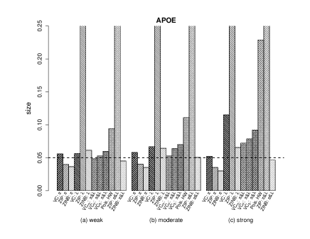
We generated data from a zero-inflated Poisson model of the form 2.1 with $\mbox{{logit}}(\pi_{i})=\alpha_{\pi}+\mathbf{X}_{i}^{\top}\boldsymbol{{\beta}}_{\pi}+\mathbf{G}_{Yi}^{\top}\boldsymbol{{\gamma}}_{\pi}$, and $\log(\lambda_{i})=\alpha_{\lambda}+\mathbf{X}_{i}^{\top}\boldsymbol{{\beta}}_{\lambda}+\mathbf{G}_{Yi}^{\top}\boldsymbol{{\gamma}}_{\lambda}$. We varied both the genetic data distribution and parameter settings across five overall simulation scenarios, the first four of which examine size of the test under the null. In setting 1), we fix the sample size at $n=1000$ but considered simple cases where $\mathbf{{X}}$ is either absent or is independent of $\mathbf{{G}}$. In setting 2), we let $\mathbf{{X}}$ to be moderately correlated with $\mathbf{{G}}$ and let the sample size $n$ = 1000, 2000 and 4000. In setting 3), we varied the correlation strength between $\mathbf{{X}}$ and $\mathbf{{G}}$, up to a maximum pairwise correlation of approximately $0.9$ to investigate the impact of correlation on the results. In setting 4), we simulated data with overdispersion by including an unobserved covariate associated with the outcome. This was to determine how robust our method is to this important deviation from the assumptions of the specified model. In setting 5), we generated data under the alternative, where the outcome was associated with (i) both $\pi_{i}$ and $\lambda_{i}$ , (ii) only with $\pi_{i}$ , and (iii) only with $\lambda_{i}$ , in order investigate how power depends on the source of the signal. Here, the covariates $\mathbf{{X}}$ were generated independent of $\mathbf{{G}}$.

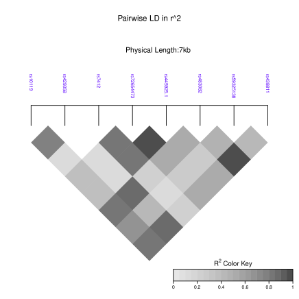
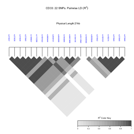
Across all scenarios to obtain genetic marker data $\mathbf{G}_{i}$ we used HAPGEN2 (Su et al.,, 2011) to generate haplotypes from 1000 genomes phase one data, CEU panel, using two representative SNP sets. First, from the APOE gene, known to be associated with our neuritic plaque burden in our example, we used the 8 SNPs in the set {rs10119, rs429358, rs7412, 19-50106239, rs445925, rs483082, rs59325138, rs438811}, and second from the CD33 gene, we used the 22 SNPs in the set {rs273637, rs273638, rs273639, rs273640, rs1399837, rs3826656, rs1710398, rs1697553, 19-56419774, rs2459141, 19-56420453, rs7245846, rs34813869, rs1354106, rs35112940, rs10409348, rs273652, rs1697531, rs169275, rs273649, rs273648, rs273646}. In either case under the alternative, 3 SNPs $G_{Yi}$ (in bold) were associated with the outcome under the true data generation model. The APOE gene has a low-moderate LD across all selected SNPs while the CD33 gene has two independent haploblocks with strong LD. We used these specific SNP sets to account for the effect of differing linkage disequilibrium (LD) structures (correlation) and genotype dimension on the performance of our method when applied to various genes.

In each scenario we compared our method to the multivariate Wald test from three models: the zero-inflated poisson, the zero-inflated negative binomial, and a simple Poisson model using the robust Huber-White (HW) variance. For each competing model except the single-parameter Poisson model, we performed multivariate Wald tests on $\widehat{\boldsymbol{\gamma}}_{\pi}$ and $\widehat{\boldsymbol{\gamma}}_{\lambda}$ separately, as well as the combined test of the vector concatenation $(\widehat{\boldsymbol{\gamma}}_{\pi}^{\top},\widehat{\boldsymbol{\gamma}}_{\lambda}^{\top})^{\top}$. For each Wald test, because Poisson, ZIP, and ZINB models failed to achieve convergence with maximum likelihood due to the collinearity in these SNP sets, in each round of our simulation we performed an LD pruning on the matrix $\mathbf{G}$, with SNPs chosen so that no pairwise correlation was above 0.99. For APOE, this LD pruning resulted in no removal of SNPs, however for CD33, this reduced the number of SNPs in the model from 22 to approximately 12, and potentially varied depending on the data.

To specify covariates, for those scenarios where $\mathbf{X}_{i}$ is independent of $\mathbf{G}_{i}$, we set $\mathbf{X}_{Ind,i}=(X_{1i},X_{2i},X_{3i},X_{4i},X_{5i})^{\top}$, where each $X_{ki}$ is a complex linear combination of independent binomial and normal random variables, with pairwise correlations that ranged from approximately 0.1 to 0.9. The complete specification is shown in the Appendix. When $\mathbf{X}_{i}$ is dependent on $\mathbf{G}_{i}$, we set $\mathbf{X}_{i,Dep}=\rho_{XG}\mathbf{A}\mathbf{G}_{Yi}+\mathbf{X}_{Ind,i}$, where the $\mathbf{X}:\mathbf{G}$ association is through a matrix $\mathbf{A}$ shown in the Appendix, and $\rho_{XG}$ is a scalar correlation strength parameter chosen to be 0.25, 0.5, or 1, representing a mild, moderate, or strong correlation, respectively. . When $\rho_{XG}=$0.25, 0.5 and 1, the maximal pairwise correlations in the $\mathbf{X}:\mathbf{G}$ correlation matrix were approximately 0.23, 0.44 and 0.64 for APOE and 0.58, 0.84, and 0.92 for CD33 respectively.

For all settings, $\alpha_{\pi}=1.5$, $\alpha_{\lambda}=1.3$, $\boldsymbol{\beta}_{\pi}=(0.75,0.5,0.25,1.0,1.0)$, $\boldsymbol{\beta}_{\lambda}=(0.25,0.5,0.75,1.0,1.0)$. For settings where $\mathbf{G}_{Yi}$ is associated with the outcome, for APOE, we set $\boldsymbol{\gamma}_{\pi}=(0.066,0.33,0.66)$, and $\boldsymbol{\gamma}_{\lambda}=(0.11,0.055,0.011)$, while for CD33, we set $\boldsymbol{\gamma}_{\pi}=(0.036,0.18,0.36)$ , and $\boldsymbol{\gamma}_{\lambda}=(0.06,0.03,0.006)$. Depending on the gene, the dimension of $\mathbf{G}_{i}$ was either $p=8$ or $p=22$, but in each case there were 3 SNPs $\mathbf{G}_{Yi}$ associated with $Y_{i}$ under the alternative, while the rest were not included in the true association model.

For setting 4) in which the model is mis-specified due to overdispersion, the true data generating mechanism is parameterized by $\mbox{{logit}}(\pi_{i})=\alpha_{\pi}+\mathbf{X}_{i}^{\top}\boldsymbol{{\beta}}_{\pi}+\mathbf{G}_{Yi}^{\top}\boldsymbol{{\gamma}}_{\pi}$, (as above), but $\log(\lambda_{i})=\alpha_{\lambda}+\mathbf{X}_{i}^{\top}\boldsymbol{{\beta}}_{\lambda}+\mathbf{G}_{Yi}^{\top}\boldsymbol{{\gamma}}_{\lambda}+\varepsilon_{\lambda,i}$ where $\varepsilon_{\lambda,i}\sim Normal(0,0.3^{2})$.

All testing was performed using the linear kernel test statistic with $\boldsymbol{{\Psi}}(\mathbf{{G}})=\mathbf{{G}}$. In each scenario, the nominal size of the type I error is $\alpha=.05$. Unless otherwise stated, the simulated data had sample size $n=1000$.

3.1.2. Simulation Results

We first compare our proposed variance component (VC) tests of the individual parameters $\pi$ and for $\lambda$ described above (here denoted $\mbox{{VC}}{}_{\pi}$ and $\mbox{{VC}}{}_{\lambda}$) with the corresponding Wald tests from the zero-inflated Poisson model and the zero-inflated negative binomial model (denoted $\mbox{{Wald}}_{\pi,ZIP}$, $\mbox{{Wald}}_{\pi,ZINB}$, $\mbox{Wald}{}_{\lambda,ZIP}$ and $\mbox{{Wald}}_{\lambda,ZINB}$). Additionally we compared six tests of the global null: three methods of combining our tests on $\pi$ and $\lambda$, namely the min-p approach ($\mbox{{VC}}_{min}$), the Fisher’s method approach ($\mbox{{VC}}_{Fisher}$), and the variance-standardized approach ($\mbox{{VC}}_{std}$) based on the statistic $\hat{Q}_{\pi,\lambda}$ proposed in Section 2, along with the Wald test using the Huber-White robust variance from the Poisson model ($\mbox{{HW}}_{Pois}$) and the Wald tests of combined $\pi$ and $\lambda$ vector in the ZIP and ZINB settings ($\mbox{{Wald}}_{ZIP}$, $\mbox{{Wald}}_{ZINB}$).

3.1.3. Size of the tests under correct model specification

Figure 3.1. Legend for following plots of simulation results.

Figure 3.2. Empirical Sizes of different testing procedures for Setting 1) (a) without$\mathbf{{X}}$; and (b) with$\mathbf{{X}}$.

Figure 3.3. Empirical sizes of different testing procedures for Setting 2) when $n=$1000, 2000, and 4000.

Figure 3.4. Empirical sizes of different testing procedures for Setting 3) when the correlation between $\mathbf{{X}}$ and $\mathbf{{G}}$ is weak, moderate or strong.

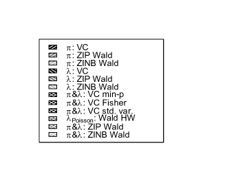
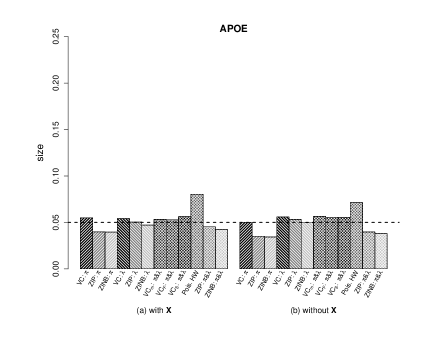
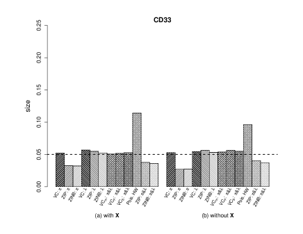
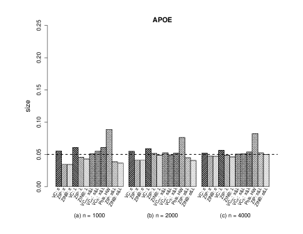
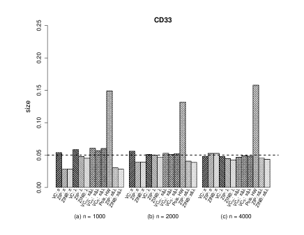
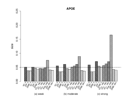
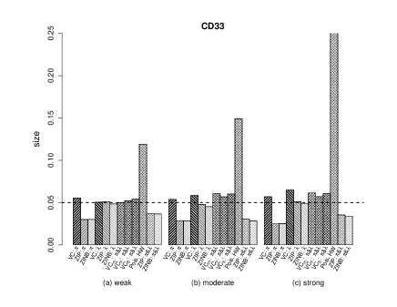
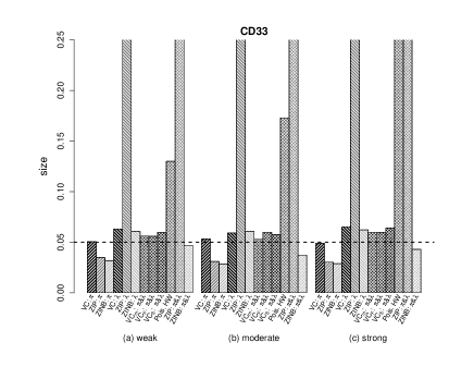
Settings 1) - 3) allow us to whether the size of the test is maintained in finite sample under correct specification of the model but with varying configurations for sample sizes and correlation structures. Results summarized in Figures 3.2, 3.3 and 3.4 suggest that type I errors of all methods except for the HW procedure are well-controlled, with empirical sizes close to the nominal $\alpha$ of 0.05 across all scenarios, under both the APOE and CD33 LD structures. The HW procedure appears to yield inflated type I errors for a majority of the settings and is thus removed from subsequent power comparisons. It is worth noting that the correlation between the covariates $\mathbf{X}_{i}$ and the tested genetic markers $\mathbf{G}_{i}$ plays relatively little role in affecting type I error of our method unless levels of correlation are quite high, e.g. where the maximal element of the $\mathbf{X}:\mathbf{G}$ correlation matrix is above 0.8.

3.1.4. Effect of mis-specification (overdispersion) on size of tests

In this scenario we investigate the robustness of different testing procedures in preserving type I errors in the presence of overdispersion and hence model mis-specification. Specifically, as described above, we included a Normally distributed covariate in the ZIP data generating model for $\lambda$ that was not controlled for in the models we used to derive the tests. We see in Figure 3.5 that the type I error of our VC test was relatively robust to overdispersion, but performance was compromised in APOE with increased $\mathbf{X}:\mathbf{G}$ correlation. As a comparison, the ZIP Wald test was badly compromised in terms of type I error with the amount of overdispersion in this setting, resulting in a sizes ranging from $0.4$ to $0.9$. Both the Wald test based on ZINB and our VC tests only have slight inflation of type I error in the presence of mis-specification due to overdispersion.

Figure 3.5. Empirical sizes of different testing procedures for Setting 4) with overdispersion and weak, moderate or strong $\mathbf{{X:G}}$ correlation.

3.1.5. Power

Figure 3.6. Power of different testing procedures when $\mathbf{{G}}$ affects (a) both mixing proportion and Poisson rate; (b) mixing proportion only; and (c) Poisson rate only.

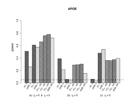
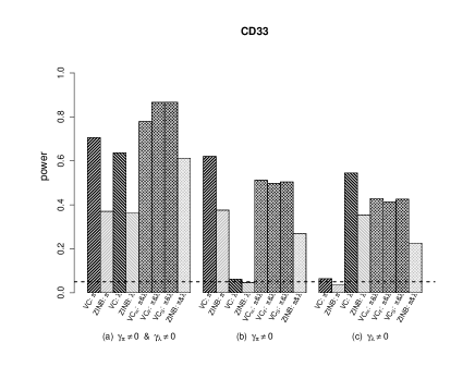
Figure 3.6 shows empirical power of different testing procedures when $\mathbf{{G}}$ is associated with (a) both $\pi$ and $\lambda$; (b) $\pi$ only; and (c) $\lambda$ only. We find that our method outperforms the competing methods on power in most scenarios, especially with those where the true signal is through the mixing proportion $\pi$ alone. There the APOE plots suggests that in some LD scenarios the power of our method can outperform the competitors when the true signal is from $\pi$, but underperform when the signal is from $\lambda$. The combined test has comparable performance to competing methods in the lower-dimensional APOE case. However in the higher dimensional CD33 scenario we find that the power of our method is consistently superior.

3.2. Data Application

3.2.1. Data Set

The ROSMAP study is a longitudinal, epidemiologic clinical-pathologic cohort study following subjects who are free of cognitive impairment at baseline. It focuses on cognition, tested annually, while also investigating correlated pathology in postmortem brain tissue analysis. Further details of the study can be found in Bennett et al. (Bennett et al.,, 2012). Genotype information was generated using the Affymetrix GeneChip 6.0 genotype platform, as described in Chibnik et al., (2011). Genotyping in the original study was limited to self-identified non-Hispanic Caucasians to reduce population heterogeneity. Remaining population heterogeneity was controlled by using the first three eigenvectors of an eigendecomposition of the genotypes. Genotypes were imputed using BEAGLE software, version 3.3.2 and 1000 Genomes Project Consortium interim phase I haplotypes, 2010-2011 data freeze. Association analysis was performed using the imputed genotype dosages.

Among 983 subjects who had died and had postmortem NP pathology measurements as well as imputed genotypes as of 2015, we restricted to the 970 subjects for whom the covariate ‘packyears at baseline’, a smoking status indicator, was recorded. We also include sex and age at death as covariates. The covariates ‘packyears at baseline’ and ‘age at death’ are included in the models as linear terms.

To illustrate the utility of our method we applied the test to several candidate genes, including ABCA7, APOE, CD33, MAPT and PTPRD, which have previously been shown to be associated with the AD risk. APOE on cytoband 19q13.32 (Zhong,, 2017) is a well known gene previously reported to be associated with Alzheimer’s risk (Lambert,, 2013). The previously reported GWAS SNPs for APOE were rs429358, and rs7412, which we used to obtain additional SNPs in LD. The additional genes we analyzed were ABCA7 (19p13.3 ; rs3752246, rs3764650), CD33 (19q13.41; rs3865444, rs3826656), MAPT (17q21.31; rs1800547, rs3785883, rs8070723) and PTPRD (9p23; rs560380, rs3764650). These genes and SNPs have also been found to be associated with Alzheimer’s (Lambert,, 2013; Giri et al.,, 2016). The previously reported GWAS SNPs for CD33 were rs3865444, rs3826656. To select a SNP set for analysis we started with all BEAGLE imputed SNPs lying within the boundaries of the gene along with those $\pm 10000$ bp upstream and downstream. We restricted to those SNPs which matched the candidate gene on the flag ‘ensembl_gene_id’ in the Ensembl.org GRCh38.11 data. We further restricted to SNPs with a variance equivalent to an MAF of 0.01 or above. We also restricted to SNPs that were in LD, with correlation ranging from 0.4 to 0.95, with SNPs previously reported to be significantly associated with the AD case-control phenotype in GWAS. These restrictions yields 8 SNPs for APOE and 22 for CD33.

Figure 3.7. Histogram of NP outcome

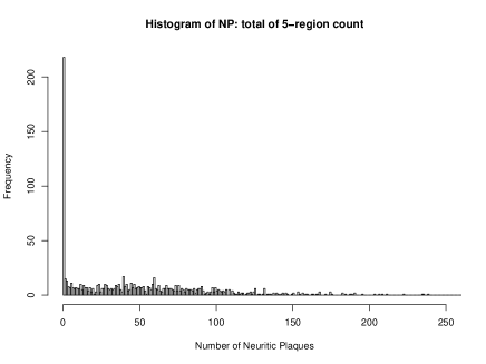
The phenotype outcome we analyze is a total count measure of neuritic plaques (NP), taken from five sites: hippocampus CA1, entorhinal cortex, inferior parietal cortex, midfrontal cortex, and midtemporal cortex. The site-specific counts are recorded by a technician who observes tissue pathology slides from each site, and are then summed to obtain a total count. The total count shows evidence of both zero-inflation and overdispersion (see figure 3.7).

3.2.2. Data Analysis Results

In Table 1, we present p-values for these genes obtained based on our proposed VC test as well as the ZINB Wald test. Other competing tests were excluded from this analysis due to their susceptibility to inflated type I error. We take $\alpha=0.05$ as the nominal size.

	$\pi$: VC	$\pi$: ZINB Wald	$\lambda$: VC	$\lambda$: ZINB Wald	$\pi\&\lambda$: VC std.	$\pi\&\lambda$: ZINB
ABCA7	2.1E-01	2.1E-02	1.9E-01	6.6E-01	1.8E-01	1.1E-01
APOE	1.1E-08	2.0E-06	1.6E-06	1.4E-08	5.8E-12	4.4E-13
CD33	3.5E-01	6.7E-01	9.9E-01	3.9E-01	7.4E-01	5.8E-01
MAPT	7.7E-01	8.5E-01	4.1E-01	8.6E-01	6.7E-01	9.4E-01
PTPRD	4.0E-01	7.6E-01	3.0E-04	2.7E-01	1.6E-03	5.2E-01

Table 1. Data analysis results: p-values of selected genes in ROSMAP data

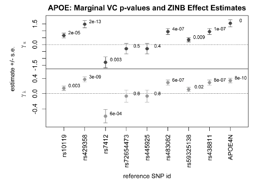
Looking at the results from our proposed method, significant p-values for APOE are consistent with past studies which have shown it to be strongly related to Alzheimers risk. We note that the p-value associated with $\lambda$ is more extreme than that for $\pi$. Thus the evidence that APOE is associated with total count of neuritic plaques appears to be stronger than the evidence APOE is associated with the presence or absence of plaques. Note however, that at least part of this discrepancy can be accounted by relative power in the tests for $\pi$ and $\lambda$, which may be affected both by effect size and by different statistical considerations for each parameter. For example it is well known that in tests of binary regression, power is a function of $\pi$, with lower power as $\pi$ approaches 0 or 1, and the same pattern is expected to hold here. By contrast, a strong association signal in $\pi$ but not $\lambda$ might suggest that the biological mechanism is ‘all-or-nothing’, meaning it may prevent or allow formation of neuritic plaques, but does not affect the rate of plaque formation if it occurs. However, we caution against making any conclusions of this sort solely based on p-values.

To illustrate the breakdown of genetic effects within a SNP set, we performed ZINB regression for the NP outcome to estimate genetic effects through $\pi$ and $\lambda$ for each SNP in APOE, using a single-SNP marginal model approach (but still controlling for the above-mentioned covariates). We also computed the effect estimate for the regression against the APOE $\varepsilon 4$ allele count, to compare results for individual SNPs with those for this well-known haplotype. In Figure 3.8 we report the maximum likelihood estimates of genetic effects $\gamma_{\pi}$ and $\gamma_{\lambda}$, along with their standard errors, and the corresponding $\mbox{{VC}}_{\pi}$ or $\mbox{{VC}}_{\lambda}$ p-value. Results for previously reported GWAS snps rs429358, and rs7412 show a strong signal in our analysis in both $\pi$ and $\lambda$.

Farebrother’s method (Farebrother,, 1984), implemented in the R statistical software package ‘CompQuadForm’, was used to calculate the the distribution of $\hat{Q}_{\iota}$ in both the marginal and the gene-level data application in order to obtain additional precision for the p-values. Nevertheless, the p-value was calculated as 0 for the test of $\pi$ for the APOE $\varepsilon 4$ allele .

Figure 3.8. Plot of APOE SNP and APOE-$\varepsilon$4 haplotype effects from marginal models

4. Discussion

We have derived novel VC tests that can efficiently detect the association between a set of genetic markers and a zero-inflated count outcome. We have shown the test to adequately control type I error in many simulation scenarios and have shown our method to obtain superior power to competing tests especially with large or sparse sets of markers with certain LD structures. Additionally we have seen that the proposed method has feasible application to genomic data from an Alzheimer’s data study. The proposed VC testing procedures appear to adequately control type I error in all of the correctly specified simulation settings we investigated. The test is also not sensitive to the presence of model mis-specification due to overdispersion, which is of practical importance. This is in part due to the use of perturbation resampling for ascertaining asymptotic distribution. Even under model mis-specification, provided that $\mathbf{{X}}$ is independent of $\mathbf{{G}}$, our proposed procedure can be shown to preserve the type I error.

The standard GWAS remains one that considers testing individual SNPs separately. It is possible to take this marginal approach using our method. However, we believe that the potential to combine SNP effects at the gene level is likely to increase power in many circumstances. The linear model proposed in this paper to test the association of individual genes with a ZIP phenotype is probably adequate for a proportion of such associations, in particular we detect a signal in the APOE gene, despite not explicitly coding the APOE $\varepsilon 2,$ $\varepsilon 3$, and $\varepsilon 4$ haplotypes but instead using additive SNP effects. However, if it is important to capture interactions or other complex SNP effects, our method easily admits a generalization which makes this possible.

With proper choices of $\mathbf{\boldsymbol{{\Psi}}(\cdot)}$, our proposed procedure corresponds to a kernel machine score test that can be used to detect non-linear effects. Specifically, suppose $h_{\iota}(\mathbf{{G}})\in\mathcal{{H}}_{K}$ with $\mathcal{{H}}_{K}=\mbox{{span}$\left\{\psi_{\ell}(\mathbf{{G}\cdot}),\ell=1,...,\mathcal{{J}}\right\}$ }$ being a reproducible kernel space generated by a given positive definite kernel function $K(\cdot,\cdot)$ (Cristianini and Shawe-Taylor,, 2000). Then letting $\boldsymbol{{\Psi}}(\cdot)=[\psi_{\ell}(\cdot),...,\psi_{\mathcal{{J}}}(\cdot)]^{\top}$ leads to a score test of the form $\hat{\mathbf{r}}_{\iota}^{\top}\mathbb{{K}}\hat{\mathbf{r}}_{\iota}$, where $\hat{\mathbf{r}}_{\iota}=(\hat{{r}}_{\iota,1},...,\hat{{r}}_{\iota,n})^{\top}$and $\mathbb{{K}}=[K(\mathbf{{G}}_{i},\mathbf{{G}}_{j})]_{n\times n}$ is the observed kernel matrix. Intuitively $K(\cdot,\cdot)$ defines a measure of genetic similarity between different subjects’ genotypes. Moreover, this transformation projects the original genotype information via a nonlinear transformation to a larger function space which can be incorporated into the model linearly. Different choices of kernel (see Wu et al.,, 2010) allow different bases for the non-parametric function modeling the association between the ZIP outcome and the $q$ markers in the SNP set, in turn allowing for power to test complex relationships and interactions.

Appendix 1: asymptotic distribution

We next outline the key steps for deriving the asymptotic distribution for $\sqrt{{n}}\hat{\mathbf{{S}}}\equiv\sqrt{{n}}(\hat{\mathbf{{S}}}_{\pi}^{\top},\hat{\mathbf{{S}}}_{\lambda}^{\top})^{\top}$ under $H_{0}$. To this end, we write $\hat{\mathbf{{S}}}_{\iota}=\widetilde{{\mathbf{S}}}_{\iota}(\widehat{{\boldsymbol{{\beta}}}}_{0})$ and $\bar{\mathbf{{S}}}_{\iota}=\widetilde{{\mathbf{S}}}_{\iota}(\boldsymbol{{\beta}}_{0})=n^{-1}\sum r_{\iota,i}\mathbf{\mathbf{\boldsymbol{\Psi}(}G}_{i})$, where $\widetilde{{\mathbf{S}}}_{\iota}(\boldsymbol{{\beta}})=n^{-1}\sum r_{\iota}(Y_{i},\mathbf{X}_{i}^{\top}\boldsymbol{{\beta}}_{\pi},\mathbf{X}_{i}^{\top}\boldsymbol{{\beta}}_{\lambda})\mathbf{\mathbf{\boldsymbol{\Psi}(}G}_{i})$, and $r_{\iota,i}=r_{\iota}(Y_{i},\mathbf{X}_{i}^{\top}\boldsymbol{{\beta}}_{0,\pi},\mathbf{X}_{i}^{\top}\boldsymbol{{\beta}}_{0,\lambda})$ First, by a standard law of large numbers and properties of the maximum likelihood estimator, we have $\widehat{{\boldsymbol{{\beta}}}}_{0}\to{\boldsymbol{{\beta}}}_{0}$ in probability and $\sqrt{{n}}(\widehat{{\boldsymbol{{\beta}}}}_{0}-{\boldsymbol{{\beta}}}_{0})=n^{-1/2}\sum_{i=1}^{n}\{(\mathbb{\mathbf{\mathbb{{I}}}}_{\pi}^{-1}\mathbf{{U}}_{\pi,i})^{\top},(\mathbb{\mathbf{\mathbb{{I}}}}_{\lambda}^{-1}\mathbf{{U}}_{\lambda,i})^{\top}\}^{\top}+o_{p}(1)$ which converges in distribution to a zero-mean multivariate normal. On the other hand, it follows from a uniform law of large numbers (Pollard,, 1990) that $\widetilde{{\mathbf{S}}}_{\iota}(\boldsymbol{{\beta}})-\mathbf{{s}}_{\iota}(\boldsymbol{{\beta}})\to 0$ in probability uniformly in $\boldsymbol{{\beta}}$, where $\mathbf{{s}}_{\iota}(\boldsymbol{{\beta}})=E\left\{{r_{\iota}(Y_{i},\mathbf{X}_{i}^{\top}\boldsymbol{{\beta}}_{\pi},\mathbf{X}_{i}^{\top}\boldsymbol{{\beta}}_{\lambda})\mathbf{G}_{i}}\right\}$. Therefore, $|\hat{\mathbf{{S}}}_{\iota}|=|\hat{\mathbf{{S}}}_{\iota}-\mathbf{{s}_{\iota}}({\boldsymbol{{\beta}}}_{0})|\leq\sup_{\boldsymbol{{\beta}}}|\widetilde{{\mathbf{S}}}_{\iota}(\boldsymbol{{\beta}})-\mathbf{{s}_{\iota}(\boldsymbol{{\beta}})}|+|\mathbf{{s}_{\iota}(\widehat{{\boldsymbol{{\beta}}}}_{0})}-\mathbf{{s}}_{\iota}({\boldsymbol{{\beta}}}_{0})|\to 0$ in probability. The first equality is due to the fact that $\mathbf{{s}}_{\iota}({\boldsymbol{{\beta}}}_{0})=0$, which can be verified as follows:

$$E\left[r_{\pi,i}\right] \equiv E\left[I_{Y_{i}=0}\frac{P(Y_{i}>0)}{P(Y_{i}=0)}(1-\pi_{0,i})-I_{Y_{i}>0}(1-\pi_{0,i})\right]$$

$$= P(Y_{i}>0)(1-\pi_{0,i})-P(Y_{i}>0)(1-\pi_{0,i})=0$$

$$E\left[r_{\lambda,i}\right] \equiv E\left[I_{Y_{i}=0}\frac{\lambda_{0,i}\pi_{0,i}exp(-\lambda_{0,i})}{P(Y_{i}=0)}-I_{Y_{i}>0}(Y_{i}-\lambda_{0,i})\right]$$

$$= \left(\frac{\lambda_{0,i}\pi_{0,i}exp(-\lambda_{0,i})}{P(Y_{i}=0)}\right)P(Y_{i}=0)-\left(E[Y_{i}I_{Y_{i}>0}]-\lambda_{0,i}E[I_{Y_{i}>0}]\right)$$

$$= \lambda_{0,i}\pi_{0,i}e^{-\lambda_{0,i}}-\lambda_{0,i}\pi_{0,i}+\lambda_{0,i}\pi_{0,i}(1-e^{-\lambda_{0,i}})=0.$$

To establish the asymptotic distribution for $\sqrt{{n}}\hat{\mathbf{{S}}}$, we first note that by the functional central limit theorem (Pollard,, 1990), $\sqrt{{n}}\{\widetilde{{\mathbf{S}}}(\boldsymbol{{\beta}})-\mathbf{{s}}(\boldsymbol{{\beta}})\}$ converges weakly to a zero-mean Gaussian process and thus is equicontinuous in $\boldsymbol{{\beta}}$. This, together with a Taylor series expansion, implies that

$$\begin{array}[]{ccl}\sqrt{n}\hat{\mathbf{S}}_{\iota}&\equiv&\sqrt{n}\left\{\widetilde{{\mathbf{S}}}_{\iota}(\widehat{{\boldsymbol{{\beta}}}}_{0})-\mathbf{\widetilde{{\mathbf{S}}}_{\iota}({\boldsymbol{{\beta}}}_{0})}\right\}+\sqrt{n}\bar{{\mathbf{{S}}}_{\iota}}\\ &=&\sqrt{n}(\rho_{\iota,\pi},\rho_{\iota,\lambda})(\widehat{{\boldsymbol{{\beta}}}}_{0}-{\boldsymbol{{\beta}}}_{0})+\sqrt{n}\bar{{\mathbf{{S}}}_{\iota}}\\ &=&n^{-1/2}\sum_{i}\left\{\rho_{\iota,\pi}\mathbb{\mathbf{\mathbb{{I}}}}_{\pi}^{-1}\mathbf{{U}}_{\pi,i}+\rho_{\iota,\lambda}\mathbb{\mathbf{\mathbb{{I}}}}_{\lambda}^{-1}\mathbf{{U}}_{\lambda,i}+r_{\iota,i}\mathbf{\mathbf{\boldsymbol{\Psi}(}G}_{i})\right\}+o_{p}(1).\end{array}$$

It then follows from a central limit theorem that$\sqrt{n}\hat{\mathbf{S}}$ converges in distribution to a multivariate normal distribution $MVN(\mathbf{0},\boldsymbol{{\Sigma}})$.

One can show that if $\mathbf{S}\sim MVN(\mathbf{0},\boldsymbol{\Sigma})$, then $\mathbf{S}^{\top}\mathbf{S}$ has an asymptotic distribution as a linear combination of independent $\chi_{1}^{2}$ random variables. For completeness, we sketch the argument here. First note $\mathbf{S}^{\top}\mathbf{S}=\left(\mathbf{S}^{\top}\boldsymbol{\Sigma}^{-\frac{1}{2}}\right)\boldsymbol{\Sigma}\left(\boldsymbol{\Sigma}^{-\frac{1}{2}}\mathbf{S}\right)$ so we can write $\mathbf{S}^{\top}\mathbf{S}=\mathbf{U}^{\top}\boldsymbol{\Sigma}\mathbf{U}$ where $\mathbf{U}=\boldsymbol{\Sigma}^{-\frac{1}{2}}\mathbf{S}\sim MVN(\mathbf{0},I_{p\times p})$. Then find the spectral decomposition $\boldsymbol{\Sigma}=\mathbf{A}^{\top}\boldsymbol{\Lambda}\mathbf{A}$, where $\boldsymbol{\Lambda}$ is diagonal and $\mathbf{A}^{\top}\mathbf{A}=\mathbf{A}\mathbf{A}^{\top}=I_{p\times p}$. Hence for $\mathbf{V}=\mathbf{A}\mathbf{U}$, $Var[\mathbf{V}]=\mathbf{A}Var[\mathbf{U}]\mathbf{A}^{\top}=\mathbf{A}\mathbf{A}^{\top}=I$. So $\mathbf{V}$ is multivariate normal with identity covariance, and the $k^{th}$ element of $\mathbf{V}$, $V_{k}$ is standard normal. So we have $\mathbf{S}^{\top}\mathbf{S}=\mathbf{V}^{\top}\Lambda\mathbf{V}=\sum_{k}\lambda_{k}V_{k}\cdot V_{k}=\sum_{k}\lambda_{k}\chi_{1}^{2}$.

Appendix 2: simulation settings

Specification of $\mathbf{X}_{i}=(X_{1i},X_{2i},X_{3i},X_{4i},X_{5i})^{\top}$:

$X_{1i}\sim binomial(k=2,p=0.5)$

$W_{2i}\sim binomial(2,0.5)$, $Z_{2i}\sim normal(\mu=0,\sigma^{2}=.25)$

$X_{2i}=0.5(W_{2})+Z_{2}$

$Z_{3i}\sim normal(\mu=0,\sigma^{2}=.25))$

$X_{3i}\sim 0.1X_{1i}X_{2i}+Z_{3i}$

$W_{4i}\sim binomial(2,0.4)$, $Z_{4i}\sim normal(\mu=0,\sigma^{2}=.25)$

$X_{4i}=0.1(W_{4i})-0.2(X_{2i})+0.2(X_{3i})+Z_{4i}$

$W_{5i}\sim 0.5(binomial(n,2,0.4)$, $Z_{5i}\sim normal(\mu=0,\sigma^{2}=.25)$

$X_{5}=0.5(W_{5i})+0.15(X_{2i})+0.2(X_{3i})+Z_{5i}$

Genotype-Covariate Dependence Matrix:

$A=\left[\begin{array}[]{ccccc}0.08&0.5&0.0&0.5&0.8\\ 0.09&0.4&0.1&0.0&0.0\\ 0.0&0.0&0.3&0.6&0.9\end{array}\right]$

Appendix 3: table of results

	Simulation Setting	$\pi$: VC	$\pi$: ZIP Wald	$\pi$: ZINB Wald	$\lambda$: VC	$\lambda$: ZIP Wald	$\lambda$: ZINB Wald	$\pi\&\lambda$: VC min-p	$\pi\&\lambda$: VC Fisher’s	$\pi\&\lambda$: VC std.	$\lambda_{Poisson}$: Wald HW	$\pi\&\lambda$: ZIP	$\pi\&\lambda$: ZINB
1	1a: APOE with X	0.055	0.040	0.040	0.054	0.050	0.047	0.053	0.053	0.056	0.080	0.045	0.042
2	1b: APOE without X	0.050	0.035	0.034	0.056	0.053	0.050	0.056	0.056	0.055	0.071	0.040	0.038
3	2a: APOE N = 1000	0.055	0.035	0.034	0.061	0.046	0.043	0.051	0.055	0.061	0.089	0.039	0.037
4	2b: APOE N = 2000	0.055	0.041	0.041	0.059	0.051	0.049	0.052	0.049	0.052	0.076	0.045	0.041
5	2c: APOE N = 4000	0.052	0.047	0.047	0.056	0.049	0.046	0.050	0.051	0.054	0.082	0.052	0.050
6	3a: APOE low corr.	0.051	0.038	0.037	0.050	0.047	0.044	0.046	0.045	0.048	0.075	0.041	0.039
7	3b: APOE mod. corr.	0.055	0.035	0.034	0.061	0.046	0.043	0.051	0.055	0.061	0.089	0.039	0.037
8	3c: APOE high corr.	0.059	0.035	0.035	0.071	0.054	0.051	0.056	0.063	0.071	0.165	0.042	0.040
9	4a: APOE OD low corr.	0.056	0.040	0.036	0.056	0.391	0.061	0.048	0.053	0.060	0.094	0.280	0.045
10	4b: APOE OD mod. corr.	0.058	0.040	0.035	0.067	0.487	0.064	0.053	0.064	0.070	0.111	0.376	0.050
11	4c: APOE OD high corr.	0.052	0.035	0.030	0.115	0.847	0.066	0.072	0.079	0.092	0.229	0.765	0.046
12	5a: APOE Alt. $\pi\&\lambda$	0.509	0.262	0.260	0.609	0.589	0.574	0.661	0.759	0.780	0.909	0.730	0.722
13	5b: APOE Alt. $\pi$	0.390	0.218	0.216	0.058	0.051	0.048	0.290	0.295	0.303	0.261	0.159	0.153
14	5c: APOE Alt. $\lambda$	0.062	0.035	0.035	0.481	0.553	0.539	0.363	0.362	0.377	0.412	0.408	0.399
15	1a: CD33 with X	0.052	0.033	0.032	0.057	0.055	0.052	0.051	0.052	0.053	0.114	0.038	0.036
16	1b: CD33 without X	0.053	0.027	0.027	0.054	0.056	0.053	0.054	0.056	0.055	0.096	0.040	0.037
17	2a: CD33 N = 1000	0.054	0.029	0.028	0.058	0.048	0.045	0.061	0.057	0.060	0.149	0.030	0.028
18	2b: CD33 N = 2000	0.056	0.039	0.039	0.051	0.050	0.047	0.053	0.051	0.052	0.132	0.041	0.039
19	2c: CD33 N = 4000	0.048	0.053	0.053	0.048	0.044	0.042	0.047	0.049	0.048	0.158	0.045	0.043
20	3a: CD33 corr. low	0.055	0.030	0.030	0.051	0.051	0.048	0.050	0.052	0.054	0.119	0.037	0.037
21	3b: CD33 corr. mod.	0.054	0.029	0.028	0.058	0.048	0.045	0.061	0.057	0.060	0.149	0.030	0.028
22	3c: CD33 corr. high	0.057	0.025	0.025	0.065	0.051	0.049	0.061	0.057	0.060	0.339	0.035	0.034
23	4a: CD33 OD corr. low	0.050	0.035	0.032	0.063	0.417	0.061	0.056	0.056	0.060	0.130	0.281	0.047
24	4b: CD33 OD corr. mod.	0.053	0.031	0.028	0.059	0.593	0.061	0.053	0.060	0.058	0.173	0.450	0.037
25	4c: CD33 OD corr. high	0.049	0.030	0.029	0.065	0.920	0.062	0.060	0.060	0.064	0.323	0.847	0.043
26	5a: CD33 Alt. $\pi\&\lambda$	0.705	0.370	0.370	0.636	0.372	0.362	0.779	0.866	0.867	0.747	0.621	0.612
27	5b: CD33 Alt. $\pi$	0.620	0.377	0.376	0.062	0.050	0.047	0.512	0.497	0.504	0.249	0.276	0.270
28	5c: CD33 Alt. $\lambda$	0.064	0.035	0.035	0.545	0.366	0.354	0.429	0.412	0.426	0.300	0.234	0.226

Table 1: Table of p-value results. See text for detailed descriptions of simulation scenarios.

Supplement 1: gene SNP sets

Gene sets for simulations and data analysis:

ABCA7 [46 SNPs]

rs930232, rs930231, rs3848640, rs3764642, rs4147904, rs3764645, rs4622634, rs4147909, rs3752237, rs4147912, rs4147914, rs7408475, rs12151021, rs3764651, rs3764652, rs3829687, rs3752242, rs3752243, rs3745842, rs11671895, rs881768, rs3752246, rs2279796, rs2868065, rs10411696, rs11671157, rs4147922, rs4147923, rs1968456, rs4147924, rs558820627, rs4807499, rs4147930, rs4147931, rs4147932, rs1609436, rs4147934, rs4147936, rs2242437, rs2242436, rs4147938, rs905149, rs12981369, rs1610096, rs3764653, rs1801284

APOE [8 SNPs]

rs10119, rs429358, rs7412, rs72654473, rs445925, rs483082, rs59325138, rs438811

CD33 [22 SNPs]

rs273637, rs273638, rs273639, rs273640, rs1399837, rs3826656, rs1710398, rs1697553, rs3865444, rs2459141, rs2455069, rs7245846, rs34813869, rs1354106, rs35112940, rs10409348, rs273652, rs1697531, rs169275, rs273649, rs273648, rs273646

MAPT [62 SNPs]

rs7210728, rs4792891, rs9303523, rs28646281, rs1560312, rs3785879, rs9915721, rs9899833, rs3785880, rs8080903, rs1560313, rs9904290, rs1001945, rs8078967, rs2435205, rs242557, rs242562, rs878918, rs242554, rs2664006, rs9896485, rs10514889, rs1800547, rs754593, rs6503453, rs713522, rs2471737, rs2435200, rs2435201, rs8067056, rs12946693, rs56087321, rs41543317, rs62062273, rs916896, rs7521, rs7220988, rs8070723, rs3744456, rs66660193, rs71375325, rs3785883, rs2435206, rs2435207, rs7209707, rs63750072, rs2435209, rs2435210, rs2435211, rs11568305, rs7216893, rs2435202, rs73317025, rs73317026, rs11079728, rs41543512, rs60969130, rs66499584, rs67676322, rs16940797, rs11652638, rs1078997

PTPRD [62 SNPs]

rs408960, rs324512, rs324513, rs324514, rs192973, rs635725, rs493588, rs634921, rs634098, rs580780, rs324481, rs324482, rs324483, rs324484, rs324485, rs182720, rs324486, rs324487, rs324488, rs324474, rs324475, rs324476, rs324478, rs324479, rs324480, rs526677, rs526675, rs324473, rs324472, rs324470, rs324469, rs324468, rs484454, rs674362, rs369166, rs523872, rs500091, rs2784543, rs2777489, rs3004230, rs828405, rs448616, rs557369, rs324465, rs172863, rs324466, rs324467, rs472324, rs324543, rs324542, rs10759040, rs324546, rs324545, rs324544, rs560380, rs324541, rs324540, rs1373806, rs324548, rs17666445, rs2007138, rs436929

8 imputed SNPs in APOE:

{rs10119, rs429358, rs7412, 19-50106239, rs445925, rs483082, rs59325138, rs438811}

(3 SNPs, $G_{Yi}$ (in bold), were associated with the outcome in the simulated data.)

Figure 4.1. LD structure of selected APOE SNPs: HAPGEN Data

Figure 4.2. LD structure of selected APOE SNPs: ROSMAP Data

22 imputed SNPs in CD33:

{rs273637, rs273638, rs273639, rs273640, rs1399837, rs3826656, rs1710398, rs1697553, 19-56419774, rs2459141, 19-56420453, rs7245846, rs34813869, rs1354106, rs35112940, rs10409348, rs273652, rs1697531, rs169275, rs273649, rs273648, rs273646}

(3 SNPs, $G_{Yi}$ (in bold), were associated with the outcome in the simulated data.)

Figure 4.3. LD structure of selected CD33: HAPGEN data

Figure 4.4. LD structure of selected CD33 SNPs: ROSMAP Data

References

- Bennett et al., (2012) Bennett, D. A., Schneider, J. A., Buchman, A. S., Barnes, L. L., Boyle, P. A., and Wilson, R. S. (2012). Overview and findings from the rush memory and aging project. Curr Alzheimer Res, 9(6):646–663.
- Chibnik et al., (2011) Chibnik, L. B., Shulman, J. M., Leurgans, S. E., Schneider, J. A., Wilson, R. S., Tran, D., Aubin, C., Buchman, A. S., Heward, C. B., Myers, A. J., Hardy, J. A., Huentelman, M. J., Corneveaux, J. J., Reiman, E. M., Evans, D. A., Bennett, D. A., and De Jager, P. L. (2011). Cr1 is associated with amyloid plaque burden and age-related cognitive decline. Ann Neurol, 69(3):560–569.
- Cristianini and Shawe-Taylor, (2000) Cristianini, N. and Shawe-Taylor, J. (2000). An introduction to support vector machines and other kernel-based learning methods. Cambridge university press.
- Duchesne and de Micheaux, (2010) Duchesne, P. and de Micheaux, P. L. (2010). Computing the distribution of quadratic forms: Further comparisons between the liu-tang-zhang approximation and exact methods. Computational Statistics and Data Analysis, 54:858–862.
- Farebrother, (1984) Farebrother, R. (1984). Algorithm as 204: the distribution of a positive linear combination of random variables. Journal of the Royal Statistical Society. Series C (Applied Statistics), 33(3):332–339.
- Fisher, (1925) Fisher, R. A. (1925). Statistical methods for research workers. Genesis Publishing Pvt Ltd.
- Giri et al., (2016) Giri, M., Zhang, M., and Lü, Y. (2016). Genes associated with alzheimer’s disease: an overview and current status. Clinical interventions in aging, 11:665.
- Greene, (1994) Greene, W. H. (1994). Accounting for excess zeros and sample selection in poisson and negative binomial regression models.
- Huang et al., (2014) Huang, Y.-T., Vanderweele, T. J., and Lin, X. (2014). Joint analysis of snp and gene expression data in genetic association studies of complex diseases. Ann. Appl. Stat. The Annals of Applied Statistics, 8(1):352–376.
- Imhof, (1961) Imhof, J. (1961). Computing the distribution of quadratic forms in normal variables. Biometrika, 48(3/4):419–426.
- Kline and Santos, (2012) Kline, P. and Santos, A. (2012). A score based approach to wild bootstrap inference. Journal of Econometric Methods, 1(1):23–41.
- Lambert, (2013) Lambert (2013). Meta-analysis of 74,046 individuals identifies 11 new susceptibility loci for alzheimer’s disease. Nature genetics, 45:1452–1458.
- Lambert, (1992) Lambert, D. (1992). Zero-inflated poisson regression, with an application to defects in manufacturing. Technometrics, 34(1):1–14.
- Lin et al., (2011) Lin, X., Cai, T., Wu, M. C., Zhou, Q., Liu, G., Christiani, D. C., and Lin, X. (2011). Kernel machine snp-set analysis for censored survival outcomes in genome-wide association studies. Genetic Epidemiology Genet. Epidemiol., 35(7):620–631.
- Liu et al., (2008) Liu, D., Ghosh, D., and Lin, X. (2008). Estimation and testing for the effect of a genetic pathway on a disease outcome using logistic kernel machine regression via logistic mixed models. BMC Bioinformatics, 9(1):292.
- Liu et al., (2007) Liu, D., Lin, X., and Ghosh, D. (2007). Semiparametric regression of multidimensional genetic pathway data: Least-squares kernel machines and linear mixed models. Biometrics, 63(4):1079–1088.
- Parzen et al., (1994) Parzen, M. I., Wei, L. J., and Ying, Z. (1994). A resampling method based on pivotal estimating functions. Biometrika, 81(2):341–350.
- Pollard, (1990) Pollard, D. (1990). Empirical Processes: Theory and Applications. NSF-CBMS regional conference series in probability and statistics. IMS and ASA.
- Ridout et al., (2001) Ridout, M., Hinde, J., and Demétrio, C. G. (2001). A score test for testing a zero-inflated poisson regression model against zero-inflated negative binomial alternatives. Biometrics, 57(1):219–223.
- Shen and Cai, (2016) Shen, Y. and Cai, T. (2016). Identifying predictive markers for personalized treatment selection. Biometrics, 72(4):1017–1025.
- Su et al., (2011) Su, Z., Marchini, J., and Donnelly, P. (2011). Hapgen2: simulation of multiple disease snps. Bioinformatics, 27(16):2304–2305.
- Won et al., (2009) Won, S., Morris, N., Lu, Q., and Elston, R. C. (2009). Choosing an optimal method to combine p-values. Statistics in medicine, 28(11):1537–1553.
- Wu et al., (2010) Wu, M. C., Kraft, P., Epstein, M. P., Taylor, D. M., Chanock, S. J., Hunter, D. J., and Lin, X. (2010). Powerful snp-set analysis for case-control genome-wide association studies. The American Journal of Human Genetics, 86(6):929–942.
- Wu et al., (2011) Wu, M. C., Lee, S., Cai, T., Li, Y., Boehnke, M., and Lin, X. (2011). Rare-variant association testing for sequencing data with the sequence kernel association test. The American Journal of Human Genetics, 89(1):82–93.
- Zhong, (2017) Zhong, K. (2017). Locate the cytoband. https://cytob.herokuapp.com/. Accessed: 2017-09-10.