Deep Learning: An Introduction for Applied Mathematicians
Abstract
Multilayered artificial neural networks are becoming a pervasive tool in a host of application fields. At the heart of this deep learning revolution are familiar concepts from applied and computational mathematics; notably, in calculus, approximation theory, optimization and linear algebra. This article provides a very brief introduction to the basic ideas that underlie deep learning from an applied mathematics perspective. Our target audience includes postgraduate and final year undergraduate students in mathematics who are keen to learn about the area. The article may also be useful for instructors in mathematics who wish to enliven their classes with references to the application of deep learning techniques. We focus on three fundamental questions: what is a deep neural network? how is a network trained? what is the stochastic gradient method? We illustrate the ideas with a short MATLAB code that sets up and trains a network. We also show the use of state-of-the art software on a large scale image classification problem. We finish with references to the current literature.
1 Motivation
Most of us have come across the phrase deep learning. It relates to a set of tools that have become extremely popular in a vast range of application fields, from image recognition, speech recognition and natural language processing to targeted advertising and drug discovery. The field has grown to the extent where sophisticated software packages are available in the public domain, many produced by high-profile technology companies. Chip manufacturers are also customizing their graphics processing units (GPUs) for kernels at the heart of deep learning.
Whether or not its current level of attention is fully justified, deep learning is clearly a topic of interest to employers, and therefore to our students. Although there are many useful resources available, we feel that there is a niche for a brief treatment aimed at mathematical scientists. For a mathematics student, gaining some familiarity with deep learning can enhance employment prospects. For mathematics educators, slipping “Applications to Deep Learning” into the syllabus of a class on calculus, approximation theory, optimization, linear algebra, or scientific computing is a great way to attract students and maintain their interest in core topics. The area is also ripe for independent project study.
There is no novel material in this article, and many topics are glossed over or omitted. Our aim is to present some key ideas as clearly as possible while avoiding non-essential detail. The treatment is aimed at readers with a background in mathematics who have completed a course in linear algebra and are familiar with partial differentiation. Some experience of scientific computing is also desirable.
To keep the material concrete, we list and walk through a short MATLAB code that illustrates the main algorithmic steps in setting up, training and applying an artificial neural network. We also demonstrate the high-level use of state-of-the-art software on a larger scale problem.
Section 2 introduces some key ideas by creating and training an artificial neural network using a simple example. Section 3 sets up some useful notation and defines a general network. Training a network, which involves the solution of an optimization problem, is the main computational challenge in this field. In Section 4 we describe the stochastic gradient method, a variation of a traditional optimization technique that is designed to cope with very large scale sets of training data. Section 5 explains how the partial derivatives needed for the stochastic gradient method can be computed efficiently using back propagation. First-principles MATLAB code that illustrates these ideas is provided in section 6. A larger scale problem is treated in section 7. Here we make use of existing software. Rather than repeatedly acknowledge work throughout the text, we have chosen to place the bulk of our citations in Section 8, where pointers to the large and growing literature are given. In that section we also raise issues that were not mentioned elsewhere, and highlight some current hot topics.
2 Example of an Artificial Neural Network
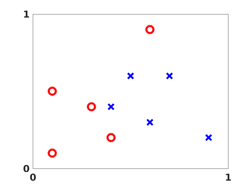
This article takes a data fitting view of artificial neural networks. To be concrete, consider the set of points shown in Figure 1. This shows labeled data—some points are in category A, indicated by circles, and the rest are in category B, indicated by crosses. For example, the data may show oil drilling sites on a map, where category A denotes a successful outcome. Can we use this data to categorize a newly proposed drilling site? Our job is to construct a transformation that takes any point in and returns either a circle or a square. Of course, there are many reasonable ways to construct such a transformation. The artificial neural network approach uses repeated application of a simple, nonlinear function.
We will base our network on the sigmoid function
| (1) |
which is illustrated in the upper half of Figure 2 over the interval . We may regard as a smoothed version of a step function, which itself mimics the behavior of a neuron in the brain—firing (giving output equal to one) if the input is large enough, and remaining inactive (giving output equal to zero) otherwise. The sigmoid also has the convenient property that its derivative takes the simple form
| (2) |
which is straightforward to verify.
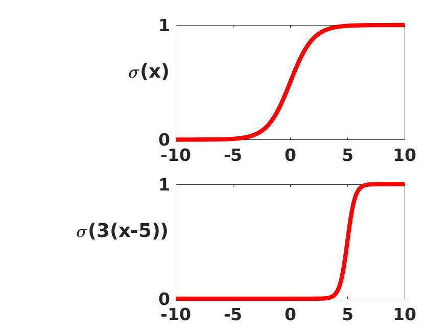
The steepness and location of the transition in the sigmoid function may be altered by scaling and shifting the argument or, in the language of neural networks, by weighting and biasing the input. The lower plot in Figure 2 shows . The factor has sharpened the changeover and the shift has altered its location. To keep our notation managable, we need to interpret the sigmoid function in a vectorized sense. For , is defined by applying the sigmoid function in the obvious componentwise manner, so that
With this notation, we can set up layers of neurons. In each layer, every neuron outputs a single real number, which is passed to every neuron in the next layer. At the next layer, each neuron forms its own weighted combination of these values, adds its own bias, and applies the sigmoid function. Introducing some mathematics, if the real numbers produced by the neurons in one layer are collected into a vector, , then the vector of outputs from the next layer has the form
| (3) |
Here, is matrix and is a vector. We say that contains the weights and contains the biases. The number of columns in matches the number of neurons that produced the vector at the previous layer. The number of rows in matches the number of neurons at the current layer. The number of components in also matches the number of neurons at the current layer. To emphasize the role of the th neuron in (3), we could pick out the th component as
where the sum runs over all entries in . Throughout this article, we will be switching between the vectorized and componentwise viewpoints to strike a balance between clarity and brevity.
In the next section, we introduce a full set of notation that allows us to define a general network. Before reaching that stage, we will give a specific example. Figure 3 represents an artificial neural network with four layers. We will apply this form of network to the problem defined by Figure 1. For the network in Figure 3 the first (input) layer is represented by two circles. This is because our input data points have two components. The second layer has two solid circles, indicating that two neurons are being employed. The arrows from layer one to layer two indicate that both components of the input data are made available to the two neurons in layer two. Since the input data has the form , the weights and biases for layer two may be represented by a matrix and a vector , respectively. The output from layer two then has the form
Layer three has three neurons, each receiving input in . So the weights and biases for layer three may be represented by a matrix and a vector , respectively. The output from layer three then has the form
The fourth (output) layer has two neurons, each receiving input in . So the weights and biases for this layer may be represented by a matrix and a vector , respectively. The output from layer four, and hence from the overall network, has the form
| (4) |

The expression (4) defines a function in terms of its parameters—the entries in the weight matrices and bias vectors. Recall that our aim is to produce a classifier based on the data in Figure 1. We do this by optimizing over the parameters. We will require to be close to for data points in category A and close to for data points in category B. Then, given a new point , it would be reasonable to classify it according to the largest component of ; that is, category A if and category B if , with some rule to break ties. This requirement on may be specified through a cost function. Denoting the ten data points in Figure 1 by , we use for the target output; that is,
| (5) |
Our cost function then takes the form
| (6) |
Here, the factor is included for convenience; it simplifies matters when we start differentiating. We emphasize that is a function of the weights and biases—the data points are fixed. The form in (6), where discrepancy is measured by averaging the squared Euclidean norm over the data points, is often refered to as a quadratic cost function. In the language of optimization, is our objective function.
Choosing the weights and biases in a way that minimizes the cost function is refered to as training the network. We note that, in principle, rescaling an objective function does not change an optimization problem. We should arrive at the same minimizer if we change to, for example, or . So the factors and in (6) should have no effect on the outcome.
For the data in Figure 1, we used the MATLAB optimization toolbox to minimize the cost function (6) over the parameters defining , , , , and . More precisely, we used the nonlinear least-squares solver lsqnonlin. For the trained network, Figure 4 shows the boundary where . So, with this approach, any point in the shaded region would be assigned to category A and any point in the unshaded region to category B.
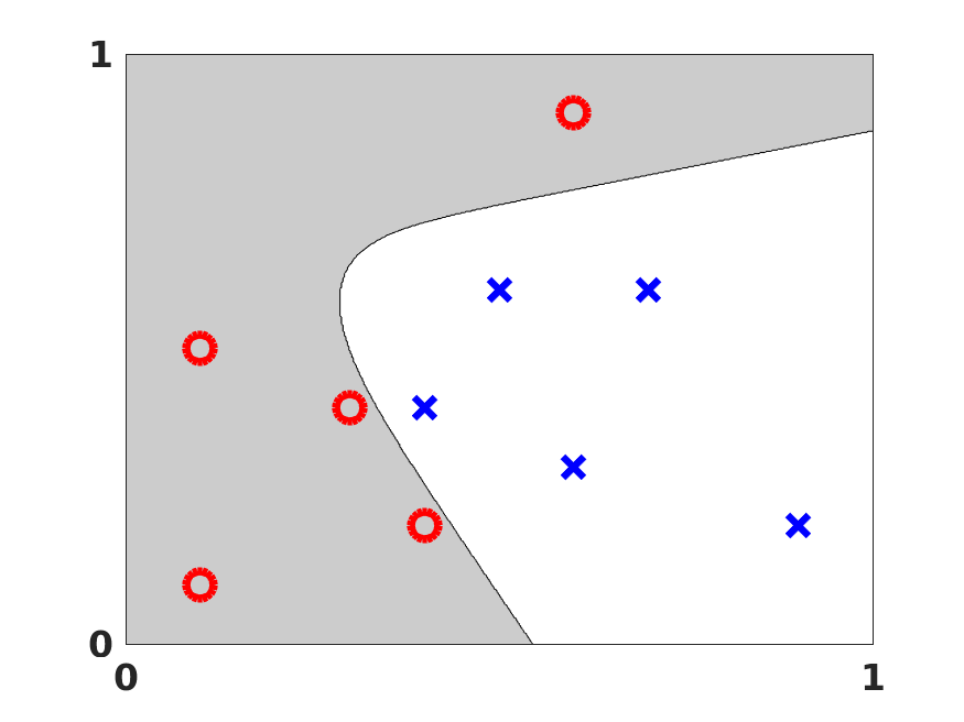
Figure 5 shows how the network responds to additional training data. Here we added one further category B point, indicated by the extra cross at , and re-ran the optimization routine.
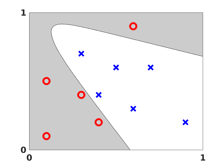
The example illustrated in Figure 4 is small-scale by the standards of today’s deep learning tools. However, the underlying optimization problem, minimizing a non-convex objective function over variables, is fundamentally difficult. We cannot exhaustively search over a 23 dimensional parameter space, and we cannot guarantee to find the global minimum of a non-convex function. Indeed, some experimentation with the location of the data points in Figure 4 and with the choice of initial guess for the weights and biases makes it clear that lsqnonlin, with its default settings, cannot always find an acceptable solution. This motivates the material in sections 4 and 5, where we focus on the optimization problem.
3 The General Set-up
The four layer example in section 2 introduced the idea of neurons, represented by the sigmoid function, acting in layers. At a general layer, each neuron receives the same input—one real value from every neuron at the previous layer—and produces one real value, which is passed to every neuron at the next layer. There are two exceptional layers. At the input layer, there is no “previous layer” and each neuron receives the input vector. At the output layer, there is no “next layer” and these neurons provide the overall output. The layers in between these two are called hidden layers. There is no special meaning to this phrase; it simply indicates that these neurons are performing intermediate calculations. Deep learning is a loosely-defined term which implies that many hidden layers are being used.
We now spell out the general form of the notation from section 2. We suppose that the network has layers, with layers and being the input and output layers, respectively. Suppose that layer , for contains neurons. So is the dimension of the input data. Overall, the network maps from to . We use to denote the matrix of weights at layer . More precisely, is the weight that neuron at layer applies to the output from neuron at layer . Similarly, is the vector of biases for layer , so neuron at layer uses the bias .
In Fig 6 we give an example with layers. Here, , , , and , so , , , , , , and .
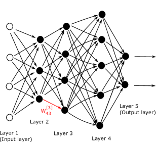
Given an input , we may then neatly summarize the action of the network by letting denote the output, or activation, from neuron at layer . So, we have
| (7) | |||||
| (8) |
It should be clear that (7) and (8) amount to an algorithm for feeding the input forward through the network in order to produce an output . At the end of section 5 this algorithm appears within a pseudocode description of an approach for training a network.
Now suppose we have pieces of data, or training points, in , , for which there are given target outputs in . Generalizing (6), the quadratic cost function that we wish to minimize has the form
| (9) |
where, to keep notation under control, we have not explicitly indicated that is a function of all the weights and biases.
4 Stochastic Gradient
We saw in the previous two sections that training a network corresponds to choosing the parameters, that is, the weights and biases, that minimize the cost function. The weights and biases take the form of matrices and vectors, but at this stage it is convenient to imagine them stored as a single vector that we call . The example in Figure 3 has a total of 23 weights and biases. So, in that case, . Generally, we will suppose , and write the cost function in (9) as to emphasize its dependence on the parameters. So .
We now introduce a classical method in optimization that is often referred to as steepest descent or gradient descent. The method proceeds iteratively, computing a sequence of vectors in with the aim of converging to a vector that minimizes the cost function. Suppose that our current vector is . How should we choose a perturbation, , so that the next vector, , represents an improvement? If is small, then ignoring terms of order , a Taylor series expansion gives
| (10) |
Here denotes the partial derivative of the cost function with respect to the th parameter. For convenience, we will let denote the vector of partial derivatives, known as the gradient, so that
Then (10) becomes
| (11) |
Our aim is to reduce the value of the cost function. The relation (11) motivates the idea of choosing to make as negative as possible. We can address this problem via the Cauchy–Schwarz inequality, which states that for any , we have . So the most negative that can be is , which happens when . Hence, based on (11), we should choose to lie in the direction . Keeping in mind that (11) is an approximation that is relevant only for small , we will limit ourselves to a small step in that direction. This leads to the update
| (12) |
Here is small stepsize that, in this context, is known as the learning rate. This equation defines the steepest descent method. We choose an initial vector and iterate with (12) until some stopping criterion has been met, or until the number of iterations has exceeded the computational budget.
Our cost function (9) involves a sum of individual terms that runs over the training data. It follows that the partial derivative is a sum over the training data of individual partial derivatives. More precisely, let
| (13) |
Then, from (9),
| (14) |
When we have a large number of parameters and a large number of training points, computing the gradient vector (14) at every iteration of the steepest descent method (12) can be prohibitively expensive. A much cheaper alternative is to replace the mean of the individual gradients over all training points by the gradient at a single, randomly chosen, training point. This leads to the simplest form of what is called the stochastic gradient method. A single step may be summarized as
-
1.
Choose an integer uniformly at random from .
-
2.
Update
(15)
In words, at each step, the stochastic gradient method uses one randomly chosen training point to represent the full training set. As the iteration proceeds, the method sees more training points. So there is some hope that this dramatic reduction in cost-per-iteration will be worthwhile overall. We note that, even for very small , the update (15) is not guaranteed to reduce the overall cost function—we have traded the mean for a single sample. Hence, although the phrase stochastic gradient descent is widely used, we prefer to use stochastic gradient.
The version of the stochastic gradient method that we introduced in (15) is the simplest from a large range of possibilities. In particular, the index in (15) was chosen by sampling with replacement—after using a training point, it is returned to the training set and is just as likely as any other point to be chosen at the next step. An alternative is to sample without replacement; that is, to cycle through each of the training points in a random order. Performing steps in this manner, refered to as completing an epoch, may be summarized as follows:
-
1.
Shuffle the integers into a new order, .
-
2.
for upto , update
(16)
If we regard the stochastic gradient method as approximating the mean over all training points in (14) by a single sample, then it is natural to consider a compromise where we use a small sample average. For some we could take steps of the following form.
-
1.
Choose integers, , uniformly at random from .
-
2.
Update
(17)
In this iteration, the set is known as a mini-batch. There is a without replacement alternative where, assuming for some , we split the training set randomly into distinct mini-batches and cycle through them.
Because the stochastic gradient method is usually implemented within the context of a very large scale computation, algorithmic choices such as mini-batch size and the form of randomization are often driven by the requirements of high performance computing architectures. Also, it is, of course, possible to vary these choices, along with others, such as the learning rate, dynamically as the training progresses in an attempt to accelerate convergence.
5 Back Propagation
We are now in a position to apply the stochastic gradient method in order to train an artificial neural network. So we switch from the general vector of parameters, , used in section 4 to the entries in the weight matrices and bias vectors. Our task is to compute partial derivatives of the cost function with respect to each and . We saw that the idea behind the stochastic gradient method is to exploit the structure of the cost function: because (9) is a linear combination of individual terms that runs over the training data the same is true of its partial derivatives. We therefore focus our attention on computing those individual partial derivatives.
Hence, for a fixed training point we regard in (13) as a function of the weights and biases. So we may drop the dependence on and simply write
| (18) |
We recall from (8) that is the output from the artificial neural network. The dependence of on the weights and biases arises only through .
To derive worthwhile expressions for the partial derivatives, it is useful to introduce two further sets of variables. First we let
| (19) |
We refer to as the weighted input for neuron at layer . The fundamental relation (8) that propagates information through the network may then be written
| (20) |
Second, we let be defined by
| (21) |
This expression, which is often called the error in the th neuron at layer , is an intermediate quantity that is useful both for analysis and computation. However, we point out that this useage of the term error is somewhat ambiguous. At a general, hidden layer, it is not clear how much to “blame” each neuron for discrepancies in the final output. Also, at the output layer, , the expression (21) does not quantify those discrepancies directly. The idea of referring to in (21) as an error seems to have arisen because the cost function can only be at a minimum if all partial derivatives are zero, so is a useful goal. As we mention later in this section, it may be more helpful to keep in mind that measures the sensitivity of the cost function to the weighted input for neuron at layer .
At this stage we also need to define the Hadamard, or componentwise, product of two vectors. If , then is defined by . In words, the Hadamard product is formed by pairwise multiplication of the corresponding components.
With this notation, the following results are a consequence of the chain rule.
Lemma 1
We have
| (22) | |||||
| (23) | |||||
| (24) | |||||
| (25) |
Proof We begin by proving (22). The relation (20) with shows that and are connected by , and hence
Also, from (18),
So, using the chain rule,
which is the componentwise form of (22).
To show (23), we use the chain rule to convert from to . Applying the chain rule, and using the definition (21),
| (26) |
Now, from (19) we know that and are connected via
Hence,
In (26) this gives
which may be rearranged as
This is the componentwise form of (23).
To show (24), we note from (19) and (20) that is connected to by
Since does not depend on , we find that
Then, from the chain rule,
Finally, to obtain (25) we start with the componentwise version of (19),
which gives
| (27) |
and
| (28) |
In words, (27) and (28) follow because the th neuron at layer uses the weights from only the th row of , and applies these weights linearly. Then, from the chain rule, (27) and (28) give
where the last step used the definition of in (21). This completes the proof.
There are many aspects of Lemma 1 that deserve our attention. We recall from (7), (19) and (20) that the output can be evaluated from a forward pass through the network, computing , , , , …, in order. Having done this, we see from (22) that is immediately available. Then, from (23), , , …, may be computed in a backward pass. From (24) and (25), we then have access to the partial derivatives. Computing gradients in this way is known as back propagation.
To gain further understanding of the back propagation formulas (24) and (25) in Lemma 1, it is useful to recall the fundamental definition of a partial derivative. The quantity measures how changes when we make a small perturbation to . For illustration, Figure 6 highlights the weight . It is clear that a change in this weight has no effect on the output of previous layers. So to work out we do not need to know about partial derivatives at previous layers. It should, however, be possible to express in terms of partial derivatives at subsequent layers. More precisely, the activation feeding into the th neuron on layer is , and, by definition, measures the sensitivity of with respect to this input. Feeding in to this neuron we have , so it makes sense that
Similarly, in terms of the bias, is feeding in to the neuron, which explains why
We may avoid the Hadamard product notation in (22) and (23) by introducing diagonal matrices. Let denote the diagonal matrix with entry given by . Then we see that and . We could expand this out as
We also recall from (2) that is trivial to compute.
The relation (24) shows that corresponds precisely to the gradient of the cost function with respect to the biases at layer . If we regard as defining the component in a matrix of partial derivatives at layer , then (25) shows this matrix to be the outer product .
Putting this together, we may write the following pseudocode for an algorithm that trains a network using a fixed number, , of stochastic gradient iterations. For simplicity, we consider the basic version (15) where single samples are chosen with replacement. For each training point, we perform a forward pass through the network in order to evaluate the activations, weighted inputs and overall output . Then we perform a backward pass to compute the errors and updates.
-
For upto
-
Choose an integer uniformly at random from
-
is current training data point
-
-
For upto
-
-
end
-
-
For downto
-
-
end
-
For downto
-
-
end
-
-
end
6 Full MATLAB Example
We now give a concrete illustration involving back propagation and the stochastic gradient method. Listing 6.1 shows how a network of the form shown in Figure 3 may be used on the data in Figure 1. We note that this MATLAB code has been written for clarity and brevity, rather than efficiency or elegance. In particular, we have “hardwired” the number of layers and iterated through the forward and backward passes line by line. (Because the weights and biases do not have the the same dimension in each layer, it is not convenient to store them in a three-dimensional array. We could use a cell array or structure array, [18], and then implement the forward and backward passes in for loops. However, this approach produced a less readable code, and violated our self-imposed one page limit.)
The function netbp in Listing 6.1 contains the nested function cost, which evaluates a scaled version of in (6). Because this function is nested, it has access to the variables in the main function, notably the training data. We point out that the nested function cost is not used directly in the forward and backward passes. It is called at each iteration of the stochastic gradient method so that we can monitor the progress of the training.
Listing 6.2 shows the function activate, used by netbp, which applies the sigmoid function in vectorized form.
At the start of netbp we set up the training data and target values, as defined in (5). We then initialize all weights and biases using the normal pseudorandom number generator randn. For simplicity, we set a constant learning rate eta = 0.05 and perform a fixed number of iterations Niter = 1e6.
We use the the basic stochastic gradient iteration summarized at the end of Section 5. Here, the command randi(10) returns a uniformly and independently chosen integer between and .
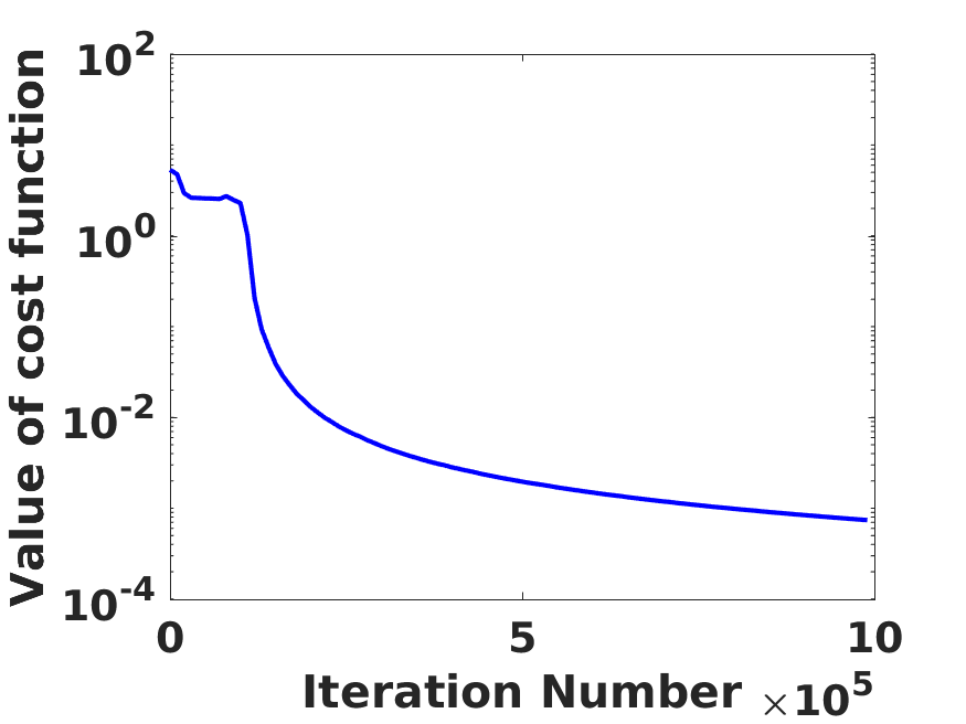
Having stored the value of the cost function at each iteration, we use the semilogy command to visualize the progress of the iteration.
In this experiment, our initial guess for the weights and biases produced a cost function value of . After stochastic gradient steps this was reduced to . Figure 7 shows the semilogy plot, and we see that the decay is not consistent—the cost undergoes a flat period towards the start of the process. After this plateau, we found that the cost decayed at a very slow linear rate—the ratio between successive values was typically within around of unity.
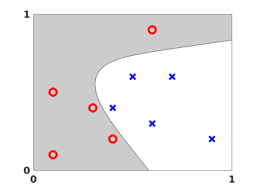
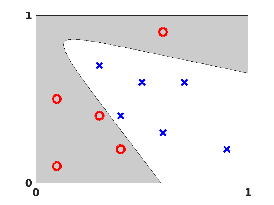
An extended version of netbp can be found in the supplementary material. This version has the extra graphics commands that make Figure 7 more readable. It also takes the trained network and produces Figure 8. This plot shows how the trained network carves up the input space. Eagle-eyed readers will spot that the solution in Figure 8. differs slightly from the version in Figure 4, where the same optimization problem was tackled by the nonlinear least-squares solver lsqnonlin. In Figure 9 we show the corresponding result when an extra data point is added; this can be compared with Figure 5.
function netbp
%NETBP Uses backpropagation to train a network
%%%%%%% DATA %%%%%%%%%%%
x1 = [0.1,0.3,0.1,0.6,0.4,0.6,0.5,0.9,0.4,0.7];
x2 = [0.1,0.4,0.5,0.9,0.2,0.3,0.6,0.2,0.4,0.6];
y = [ones(1,5) zeros(1,5); zeros(1,5) ones(1,5)];
% Initialize weights and biases
rng(5000);
W2 = 0.5*randn(2,2); W3 = 0.5*randn(3,2); W4 = 0.5*randn(2,3);
b2 = 0.5*randn(2,1); b3 = 0.5*randn(3,1); b4 = 0.5*randn(2,1);
% Forward and Back propagate
eta = 0.05; % learning rate
Niter = 1e6; % number of SG iterations
savecost = zeros(Niter,1); % value of cost function at each iteration
for counter = 1:Niter
k = randi(10); % choose a training point at random
x = [x1(k); x2(k)];
% Forward pass
a2 = activate(x,W2,b2);
a3 = activate(a2,W3,b3);
a4 = activate(a3,W4,b4);
% Backward pass
delta4 = a4.*(1-a4).*(a4-y(:,k));
delta3 = a3.*(1-a3).*(W4’*delta4);
delta2 = a2.*(1-a2).*(W3’*delta3);
% Gradient step
W2 = W2 - eta*delta2*x’;
W3 = W3 - eta*delta3*a2’;
W4 = W4 - eta*delta4*a3’;
b2 = b2 - eta*delta2;
b3 = b3 - eta*delta3;
b4 = b4 - eta*delta4;
% Monitor progress
newcost = cost(W2,W3,W4,b2,b3,b4) % display cost to screen
savecost(counter) = newcost;
end
% Show decay of cost function
save costvec
semilogy([1:1e4:Niter],savecost(1:1e4:Niter))
function costval = cost(W2,W3,W4,b2,b3,b4)
costvec = zeros(10,1);
for i = 1:10
x =[x1(i);x2(i)];
a2 = activate(x,W2,b2);
a3 = activate(a2,W3,b3);
a4 = activate(a3,W4,b4);
costvec(i) = norm(y(:,i) - a4,2);
end
costval = norm(costvec,2)^2;
end % of nested function
end
function y = activate(x,W,b) %ACTIVATE Evaluates sigmoid function. % % x is the input vector, y is the output vector % W contains the weights, b contains the shifts % % The ith component of y is activate((Wx+b)_i) % where activate(z) = 1/(1+exp(-z)) y = 1./(1+exp(-(W*x+b)));
7 Image Classification Example
We now move on to a more realistic task, which allows us to demonstrate the power of the deep learning approach. We make use of the MatConvNet toolbox [33], which is designed to offer key deep learning building blocks as simple MATLAB commands. So MatConvNet is an excellent environment for prototyping and for educational use. Support for GPUs also makes MatConvNet efficient for large scale computations, and pre-trained networks may be downloaded for immediate use.
Applying MatConvNet on a large scale problem also gives us the opportunity to outline further concepts that are relevant to practical computation. These are introduced in the next few subsections, before we apply them to the image classification exercise.
7.1 Convolutional Neural Networks
MatConvNet uses a special class of artificial neural networks known as Convolutional Neural Networks (CNNs), which have become a standard tool in computer vision applications. To motivate CNNs, we note that the general framework described in section 3 does not scale well in the case of digital image data. Consider a color image made up of 200 by 200 pixels, each with a red, green and blue component. This corresponds to an input vector of dimension , and hence a weight matrix at level 2 that has columns. If we allow general weights and biases, then this approach is clearly infeasible. CNNs get around this issue by constraining the values that are allowed in the weight matrices and bias vectors. Rather than a single full-sized linear transformation, CNNs repeatedly apply a small-scale linear kernel, or filter, across portions of their input data. In effect, the weight matrices used by CNNs are extremely sparse and highly structured.
To understand why this approach might be useful, consider premultiplying an input vector in by the matrix
| (29) |
This produces a vector in made up of differences between neighboring values. In this case we are using a filter and a stride of length one—the filter advances by one place after each use. Appropriate generalizations of this matrix to the case of input vectors arising from 2D images can be used to detect edges in an image—returning a large absolute value when there is an abrupt change in neighboring pixel values. Moving a filter across an image can also reveal other features, for example, particular types of curves or blotches of the same color. So, having specified a filter size and stride length, we can allow the training process to learn the weights in the filter as a means to extract useful structure.
The word “convolutional” arises because the linear transformations involved may be written in the form of a convolution. In the 1D case, the convolution of the vector with the filter has th component given by
The example in (29) corresponds to a filter with , and all other . In the case
| (30) |
we are applying a filter with four weights, , , , and , using a stride length of two. Because the dimension of the input vector is not compatible with the filter length, we have padded with an extra zero value.
In practice, image data is typically regarded as a three dimensional tensor: each pixel has two spatial coordinates and a red/green/blue value. With this viewpoint, the filter takes the form of a small tensor that is successsively applied to patches of the input tensor and the corresponding convolution operation is multi-dimensional. From a computational perspective, a key benefit of CNNs is that the matrix-vector products involved in the forward and backward passes through the network can be computed extremely efficiently using fast transform techniques.
A convolutional layer is often followed by a pooling layer, which reduces dimension by mapping small regions of pixels into single numbers. For example, when these small regions are taken to be squares of four neigboring pixels in a 2D image, a max pooling or average pooling layer replaces each set of four by their maximum or average value, respectively.
7.2 Avoiding Overfitting
Overfitting occurs when a trained network performs very accurately on the given data, but cannot generalize well to new data. Loosely, this means that the fitting process has focussed too heavily on the unimportant and unrepresentative “noise” in the given data. Many ways to combat overfitting have been suggested, some of which can be used together.
One useful technique is to split the given data into two distinct groups.
-
•
Training data is used in the definition of the cost function that defines the optimization problem. Hence this data drives the process that iteratively updates the weights.
-
•
Validation data is not used in the optimization process—it has no effect on the way that the weights are updated from step to step. We use the validation data only to judge the performance of the current network. At each step of the optimization, we can evaluate the cost function corresponding to the validation data. This measures how well the current set of trained weights performs on unseen data.
Intuitively, overfitting corresponds to the situation where the optimization process is driving down its cost function (giving a better fit to the training data), but the cost function for the validation error is no longer decreasing (so the performance on unseen data is not improving). It is therefore reasonable to terminate the training at a stage where no improvement is seen on the validation data.
Another popular approach to tackle overfitting is to randomly and independently remove neurons during the training phase. For example, at each step of the stochastic gradient method, we could delete each neuron with probability and train on the remaining network. At the end of the process, because the weights and biases were produced on these smaller networks, we could multiply each by a factor of for use on the full-sized network. This technique, known as dropout, has the intuitive interpretation that we are constructing an average over many trained networks, with such a consensus being more reliable than any individual.
7.3 Activation and Cost Functions
In Sections 2 to 6 we used activation functions of sigmoid form (1) and a quadratic cost function (9). There are many other widely used choices, and their relative performance is application-specific. In our image classification setting it is common to use a rectified linear unit, or ReLU,
| (31) |
as the activation.
In the case where our training data comes from labeled categories, let be the given label for data point . As an alternative to the quadratic cost function (9), we could use a softmax log loss approach, as follows. Let the output from the network take the form of a vector in such that the th component is large when the image is believed to be from category . The softmax operation
boosts the large components and produces a vector of positive weights summing to unity, which may be interpreted as probabilties. Our aim is now to force the softmax value for training point to be as close to unity as possible in component , which corresponds to the correct label. Using a logarithmic rather than quadratic measure of error, we arrive at the cost function
| (32) |
7.4 Image Classification Experiment
We now show results for a supervised learning task in
image classification.
To do this, we rely on
the codes cnn_cifar.m
and
cnn_cifar_init.m
that are available via
the
MatConvNet website.
We made only minor edits, including
some changes that allowed us
to test the use of dropout.
Hence,
in particular, we are using
the network architecture and parameter choices
from those codes.
We refer to the
MatConvNet documentation and tutorial material for
the fine details, and focus here on some of the
bigger picture issues.
We consider a set of images, each of which falls into exactly one of the following ten categories: airplane, automobile, bird, cat, deer, dog, frog, horse, ship, truck. We use labeled data from the freely available CIFAR-10 collection [20]. The images are small, having by pixels, each with a red, green, and blue component. So one piece of training data consists of values. We use a training set of 50,000 images, and use 10,000 more images as our validation set. Having completed the optimization and trained the network, we then judge its performance on a fresh collection of 10,000 test images, with 1,000 from each category.
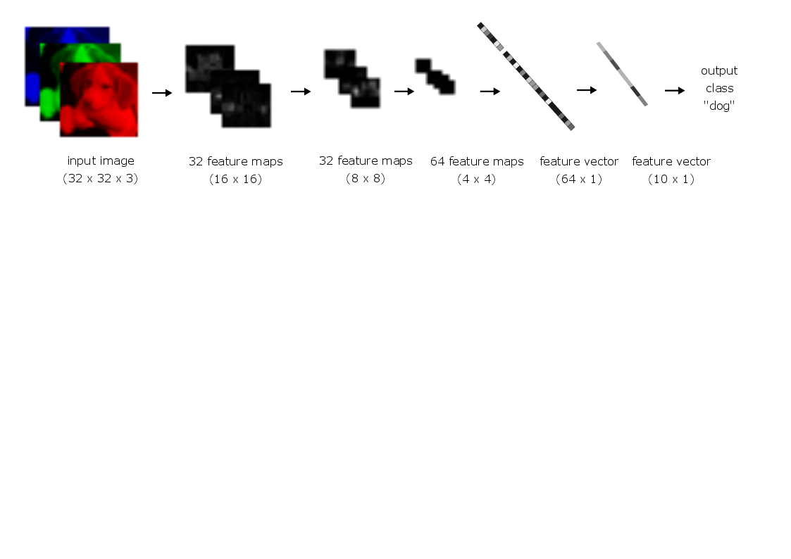
Following the architecture used in the relevant MatConvNet codes, we set up a network whose layers are divided into five blocks as follows. Here we describe the dimemsions of the inputs/outputs and weights in compact tensor notation. (Of course, the tensors could be stretched into sparse vectors and matrices in order to fit in with the general framework of sections 2 to 6. But we feel that the tensor notation is natural in this context, and it is consistent with the MatConvNet syntax.)
- Block 1
-
consists of a a convolution layer followed by a pooling layer and activation. This converts the original input into dimension . In more detail, the convolutional layer uses filters that also scan across the color channels. There are different filters, so overall the weights can be represented in a array. The output from each filter may be described as a feature map. The filters are applied with unit stride. In this way, each of the 32 feature maps has dimension . Max pooling is then applied to each feature map using stride length two. This reduces the dimension of the feature maps to . A ReLU activation is then used.
- Block 2
-
applies convolution followed by activation and then a pooling layer. This reduces the dimension to . In more detail, we use filters. Each is across the dimensions of the feature maps, and also scans across all feature maps. So the weights could be regarded as a tensor. The stride length is one, so the resulting feature maps are still of dimension . After ReLU activation, an average pooling layer of stride two is then applied, which reduces each of the feature maps to dimension .
- Block 3
-
applies a convolution layer followed by the activation function, and then performs a pooling operation, in a way that reduces dimension to . In more detail, filters are applied. Each filter is across the dimensions of the feature maps, and also scans across all feature maps. So the weights could be regarded as a tensor. The stride has length one, resulting in feature maps of dimension . After ReLU activation, an average pooling layer of stride two is applied, which reduces each of the feature maps to dimension .
- Block 4
-
does not use pooling, just convolution followed by activation, leading to dimension . In more detail, filters are used. Each filter is across the feature maps, so the weights could be regarded as a tensor, and each filter produces a single number.
- Block 5
- A final softmax
-
operation transforms each of the ten ouput components to the range .
Figure 10 gives a visual overview of the network architecture.
Our output is a vector of ten real numbers. The cost function in the optimization problem takes the softmax log loss form (32) with . We specify stochastic gradient with momentum, which uses a “moving average” of current and past gradient directions. We use mini-batches of size 100 (so in (17)) and set a fixed number of epochs. We predefine the learning rate for each epoch: , and for the first epochs, next epochs and final epochs, respectively. Running on a Tesla C2075 GPU in single precision, the 45 epochs can be completed in just under 4 hours.
As an additional test, we also train the network with dropout. Here, on each stochastic gradient step, any neuron has its output re-set to zero with independent probability
-
•
in block 1,
-
•
in block 2,
-
•
in block 3,
-
•
in block 4,
-
•
in block 5 (no dropout).
We emphasize that in this case all neurons become active when the trained network is applied to the test data.
In Figure 11 we illustrate the training process in the case of no dropout. For the plot on the left, circles are used to show how the objective function (32) decreases after each of the 45 epochs. We also use crosses to indicate the objective function value on the validation data. (More precisely, these error measures are averaged over the individual batches that form the epoch—note that weights are updated after each batch.) Given that our overall aim is to assign images to one of the ten classes, the middle plot in Figure 11 looks at the percentage of errors that take place when we classify with the highest probability choice. Similarly, the plot on the right shows the percentage of cases where the correct category is not among the top five. We see from Figure 11 that the validation error starts to plateau at a stage where the stochastic gradient method continues to make significant reductions on the training error. This gives an indication that we are overfitting—learning fine details about the training data that will not help the network to generalize to unseen data.
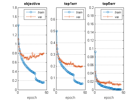
Figure 12 shows the analogous results in the case where dropout is used. We see that the training errors are significantly larger than those in Figure 11 and the validation errors are of a similar magnitude. However, two key features in the dropout case are that (a) the validation error is below the training error, and (b) the validation error continues to decrease in sync with the training error, both of which indicate that the optimization procedure is extracting useful information over all epochs.
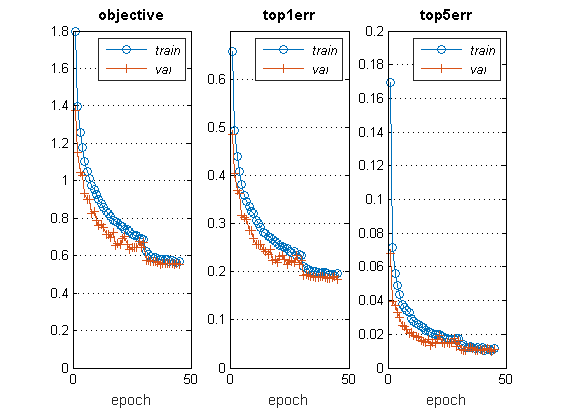
Figure 13 gives a summary of the performance of the trained network with no dropout (after 45 epochs) in the form of a confusion matrix. Here, the integer value in the general entry shows the number of occasions where the network predicted category for an image from category . Hence, off-diagonal elements indicate mis-classifications. For example, the (1,1) element equal to 814 in Figure 13 records the number of airplane images that were correctly classified as airplanes, and the (1,2) element equal to 21 records the number of automobile images that were incorrectly classified as airplanes. Below each integer is the corresponding percentage, rounded to one decimal place, given that the test data has 1,000 images from each category. The extra row, labeled “all”, summarizes the entries in each column. For example, the value 81.4% in the first column of the final row arises because 814 of the 1,000 airplane images were correctly classified. Beneath this, the value 18.6% arises because 186 of these airplane images were incorrectly classified. The final column of the matrix, also labeled “all”, summarizes each row. For example, the value 82.4% in the final column of the first row arises because 988 images were classified by the network as airplanes, with 814 of these classifications being correct. Beneath this, the value 17.6% arises because the remaining 174 out of these 988 airplane classifications were incorrect. Finally, the entries in the lower right corner summarize over all categories. We see that 80.1% of all images were correctly classified (and hence 19.9% were incorrectly classified).
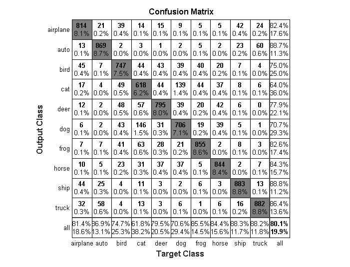
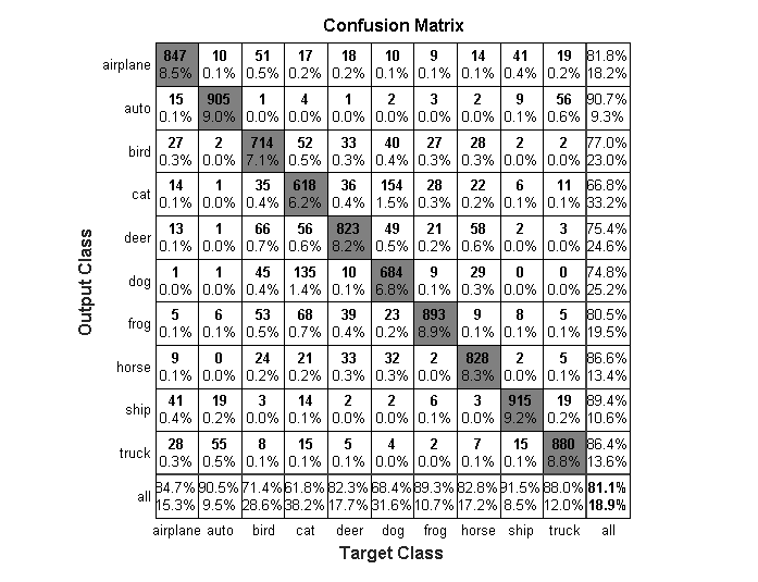
Figure 14 gives the corresponding results in the case where dropout was used. We see that the use of dropout has generally improved performance, and in particular has increased the overall success rate from 80.1% to 81.1%. Dropout gives larger values along the diagonal elements of the confusion matrix in nine out of the ten categories.
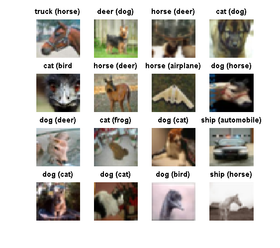
To give a feel for the difficulty of this task, Figure 15 shows 16 images randomly sampled from those that were misclassified by the non-dropout network.
8 Of Things Not Treated
This short introductory article is aimed at those who are new to deep learning. In the interests of brevity and accessibility we have ruthlessly omitted many topics. For those wishing to learn more, a good starting point is the free online book [26], which provides a hands-on tutorial style description of deep learning techniques. The survey [22] gives an intuitive and accessible overview of many of the key ideas behind deep learning, and highlights recent success stories. A more detailed overview of the prize-winning performances of deep learning tools can be found in [29], which also traces the development of ideas across more than 800 references. The review [35] discusses the pre-history of deep learning and explains how key ideas evolved. For a comprehensive treatment of the state-of-the-art, we recommend the book [10] which, in particular, does an excellent job of introducing fundamental ideas from computer science/discrete mathematics, applied/computational mathematics and probability/statistics/inference before pulling them all together in the deep learning setting. The recent review article [3] focuses on optimization tasks arising in machine learning. It summarizes the current theory underlying the stochastic gradient method, along with many alternative techniques. Those authors also emphasize that optimization tools must be interpreted and judged carefully when operating within this inherently statistical framework. Leaving aside the training issue, a mathematical framework for understanding the cascade of linear and nonlinear transformations used by deep networks is given in [24].
To give a feel for some of the key issues that can be followed up, we finish with a list of questions that may have occured to interested readers, along with brief answers and further citations.
- Why use artificial neural networks?
-
Looking at Figure 4, it is clear that there are many ways to come up with a mapping that divides the x-y axis into two regions; a shaded region containing the circles and an unshaded region containing the crosses. Artificial neural networks provide one useful approach. In real applications, success corresponds to a small generalization error; the mapping should perform well when presented with new data. In order to make rigorous, general, statements about performance, we need to make some assumptions about the type of data. For example, we could analyze the situation where the data consists of samples drawn independently from a certain probability distribution. If an algorithm is trained on such data, how will it perform when presented with new data from the same distribution? The authors in [15] prove that artificial neural networks trained with the stochastic gradient method can behave well in this sense. Of course, in practice we cannot rely on the existence of such a distribution. Indeed, experiments in [36] indicate that the worst case can be as bad as possible. These authors tested state-of-the-art convolutional networks for image classification. In terms of the heuristic performance indicators used to monitor the progress of the training phase, they found that the stochastic gradient method appears to work just as effectively when the images are randomly re-labelled. This implies that the network is happy to learn noise—if the labels for the unseen data are similarly randomized then the classifications from the trained network are no better than random choice. Other authors have established negative results by showing that small and seemingly unimportant perturbations to an image can change its predicted class, including cases where one pixel is altered [32]. Related work in [4] showed proof-of-principle for an adversarial patch, which alters the classification when added to a wide range of images; for example, such a patch could be printed as a small sticker and used in the physical world. Hence, although artificial neural networks have outperformed rival methods in many application fields, the reasons behind this success are not fully understood. The survey [34] describes a range of mathematical approaches that are beginning to provide useful insights, whilst the discussion piece [25] includes a list of ten concerns.
- Which nonlinearity?
-
The sigmoid function (1), illustrated in Figure 2, and the rectified linear unit (31) are popular choices for the activation function. Alternatives include the step function,
Each of these can undergo saturation: produce very small derivatives that thereby reduce the size of the gradient updates. Indeed, the step function and rectified linear unit have completely flat portions. For this reason, a leaky rectified linear unit, such as,
is sometimes preferred, in order to force a nonzero derivative for negative inputs. The back propagation algorithm described in section 5 carries through to general activation functions.
- How do we decide on the structure of our net?
-
Often, there is a natural choice for the size of the output layer. For example, to classify images of individual handwritten digits, it would make sense to have an output layer consisting of ten neurons, corresponding to , as used in Chapter 1 of [26]. In some cases, a physical application imposes natural constraints on one or more of the hidden layers [16]. However, in general, choosing the overall number of layers, the number of neurons within each layer, and any constraints involving inter-neuron connections, is not an exact science. Rules of thumb have been suggested, but there is no widely accepted technique. In the context of image processing, it may be possible to attribute roles to different layers; for example, detecting edges, motifs and larger structures as information flows forward [22], and our understanding of biological neurons provides further insights [10]. But specific roles cannot be completely hardwired into the network design—the weights and biases, and hence the tasks performed by each layer, emerge from the training procedure. We note that the use of back propagation to compute gradients is not restricted to the types of connectivity, activation functions and cost functions discussed here. Indeed, the method fits into a very general framework of techniques known as automatic differentiation or algorithmic differentiation [13].
- How big do deep learning networks get?
-
The AlexNet architecture [21] achieved groundbreaking image classification results in 2012. This network used 650,000 neurons, with five convolutional layers followed by two fully connected layers and a final softmax. The programme AlphaGo, developed by the Google DeepMind team to play the board game Go, rose to fame by beating the human European champion by five games to nil in October 2015 [30]. AlphaGo makes use of two artificial neural networks with 13 layers and 15 layers, some convolutional and others fully connected, involving millions of weights.
- Didn’t my numerical analysis teacher tell me never to use steepest descent?
-
It is known that the steepest descent method can perform poorly on examples where other methods, notably those using information about the second derivative of the objective function, are much more efficient. Hence, optimization textbooks typically downplay steepest descent [9, 27]. However, it is important to note that training an artificial neural network is a very specific optimization task:
-
•
the problem dimension and the expense of computing the objective function and its derivatives, can be extremely high,
-
•
the optimization task is set within a framework that is inherently statistical in nature,
-
•
a great deal of research effort has been devoted to the development of practical improvements to the basic stochastic gradient method in the deep learning context.
Currently, a theoretical underpinning for the success of the stochastic gradient method in training networks is far from complete [3]. A promising line of research is to connect the stochastic gradient method with discretizations of stochastic differential equations, [31], generalizing the idea that many deterministic optimization methods can be viewed as timestepping methods for gradient ODEs, [17]. We also note that the introduction of more traditional tools from the field of optimization may lead to improved training algorithms.
-
•
- Is it possible to regularize?
-
As we discussed in section 7, overfitting occurs when a trained network performs accurately on the given data, but cannot generalize well to new data. Regularization is a broad term that describes attempts to avoid overfitting by rewarding smoothness. One approach is to alter the cost function in order to encourage small weights. For example, (9) could be extended to
(33) Here is the regularization parameter. One motivation for (33) is that large weights may lead to neurons that are sensitive to their inputs, and hence less reliable when new data is presented. This argument does not apply to the biases, which typically are not included in such a regularization term. It is straightforward to check that using (33) instead of (9) makes a very minor and inexpensive change to the back propagation algorithm.
- What about ethics and accountability?
-
The use of “algorithms” to aid decision-making is not a recent phenomenon. However, the increasing influence of black-box technologies is naturally causing concerns in many quarters. The recent articles [7, 14] raise several relevant issues and illustrate them with concrete examples. They also highlight the particular challenges arising from massively-parameterized artificial neural networks. Professional and governmental institutions are, of course, alert to these matters. In 2017, the Association for Computing Machinery’s US Public Policy Council released seven Principles for Algorithmic Transparency and Accountability111 https://www.acm.org/ . Among their recommendations are that
-
•
“Systems and institutions that use algorithmic decision-making are encouraged to produce explanations regarding both the procedures followed by the algorithm and the specific decisions that are made”, and
-
•
“A description of the way in which the training data was collected should be maintained by the builders of the algorithms, accompanied by an exploration of the potential biases induced by the human or algorithmic data-gathering process.”
Article 15 of the European Union’s General Data Protection Regulation 2016/679222https://www.privacy-regulation.eu/en/15.htm, which takes effect in May 2018, concerns “Right of access by the data subject,” and includes the requirement that “The data subject shall have the right to obtain from the controller confirmation as to whether or not personal data concerning him or her are being processed, and, where that is the case, access to the personal data and the following information:.”Item (h) on the subsequent list covers
-
•
“the existence of automated decision-making, including profiling, referred to in Article 22(1) and (4) and, at least in those cases, meaningful information about the logic involved, as well as the significance and the envisaged consequences of such processing for the data subject.”
-
•
- What are some current research topics?
-
Deep learning is a fast-moving, high-bandwith field, where many new advances are driven by the needs of specific application areas and the features of new high performance computing architectures. Here, we briefly mention three hot-topic areas that have not yet been discussed.
Training a network can be an extremely expensive task. When a trained network is seen to make a mistake on new data, it is therefore tempting to fix this with a local perturbation to the weights and/or network structure, rather than re-training from scratch. Approaches for this type of on the fly tuning can be developed and justified using the theory of measure concentration in high dimensional spaces [12].
Adversarial networks, [11], are based on the concept that an artificial neural network may be viewed as a generative model: a way to create realistic data. Such a model may be useful, for example, as a means to produce realistic sentences, or very high resolution images. In the adversarial setting, the generative model is pitted against a discriminative model. The role of the discriminative model is to distinguish between real training data and data produced by the generative model. By iteratively improving the performance of these models, the quality of both the generation and discrimination can be increased dramatically.
The idea behind autoencoders [28] is, perhaps surprisingly, to produce an overall network whose output matches its input. More precisely, one network, known as the encoder, corresponds to a map that takes an input vector, , and produces a lower dimensional output vector . So . Then a second network, known as the decoder, corresponds to a map that takes us back to the same dimension as ; that is, . We could then aim to minimize the sum of the squared error over a set of training data. Note that this technique does not require the use of labelled data—in the case of images we are attempting to reproduce each picture without knowing what it depicts. Intuitively, a good encoder is a tool for dimension reduction. It extracts the key features. Similarly, a good decoder can reconstruct the data from those key features.
- Where can I find code and data?
-
There are many publicly available codes that provide access to deep learning algorithms. In addition to MatConvNet [33], we mention Caffe [19], Keras [5], TensorFlow [1], Theano [2] and Torch [6]. These packages differ in their underlying platforms and in the extent of expert knowledge required. Your favorite scientific computing environment may also offer a range of proprietary and user-contributed deep learning toolboxes. However, it is currently the case that making serious use of modern deep learning technology requires a strong background in numerical computing. Among the standard benchmark data sets are the CIFAR-10 collection [20] that we used in section 7, and its big sibling CIFAR-100, ImageNet [8], and the handwritten digit database MNIST [23].
Acknowledgements
We are grateful to the MatConvNet team for making their package available under a permissive BSD license. The MATLAB code in Listings 6.1 and 6.2 can be found at
http://personal.strath.ac.uk/d.j.higham/algfiles.html
as well as an exteneded version that produces Figures 7 and 8, and a MATLAB code that uses lsqnonlin to produce Figure 4.
References
- [1] M. Abadi, P. Barham, J. Chen, Z. Chen, A. Davis, J. Dean, M. Devin, S. Ghemawat, G. Irving, M. Isard, M. Kudlur, J. Levenberg, R. Monga, S. Moore, D. G. Murray, B. Steiner, P. Tucker, V. Vasudevan, P. Warden, M. Wicke, Y. Yu, and X. Zheng, TensorFlow: A system for large-scale machine learning, in 12th USENIX Symposium on Operating Systems Design and Implementation (OSDI 16), 2016, pp. 265–283.
- [2] R. Al-Rfou, G. Alain, A. Almahairi, C. Angermueller, D. Bahdanau, N. Ballas, F. Bastien, J. Bayer, A. Belikov, A. Belopolsky, Y. Bengio, A. Bergeron, J. Bergstra, V. Bisson, J. Bleecher Snyder, N. Bouchard, N. Boulanger-Lewandowski, X. Bouthillier, A. de Brébisson, O. Breuleux, P.-L. Carrier, K. Cho, J. Chorowski, P. Christiano, T. Cooijmans, M.-A. Côté, M. Côté, A. Courville, Y. N. Dauphin, O. Delalleau, J. Demouth, G. Desjardins, S. Dieleman, L. Dinh, M. Ducoffe, V. Dumoulin, S. Ebrahimi Kahou, D. Erhan, Z. Fan, O. Firat, M. Germain, X. Glorot, I. Goodfellow, M. Graham, C. Gulcehre, P. Hamel, I. Harlouchet, J.-P. Heng, B. Hidasi, S. Honari, A. Jain, S. Jean, K. Jia, M. Korobov, V. Kulkarni, A. Lamb, P. Lamblin, E. Larsen, C. Laurent, S. Lee, S. Lefrancois, S. Lemieux, N. Léonard, Z. Lin, J. A. Livezey, C. Lorenz, J. Lowin, Q. Ma, P.-A. Manzagol, O. Mastropietro, R. T. McGibbon, R. Memisevic, B. van Merriënboer, V. Michalski, M. Mirza, A. Orlandi, C. Pal, R. Pascanu, M. Pezeshki, C. Raffel, D. Renshaw, M. Rocklin, A. Romero, M. Roth, P. Sadowski, J. Salvatier, F. Savard, J. Schlüter, J. Schulman, G. Schwartz, I. V. Serban, D. Serdyuk, S. Shabanian, E. Simon, S. Spieckermann, S. R. Subramanyam, J. Sygnowski, J. Tanguay, G. van Tulder, J. Turian, S. Urban, P. Vincent, F. Visin, H. de Vries, D. Warde-Farley, D. J. Webb, M. Willson, K. Xu, L. Xue, L. Yao, S. Zhang, and Y. Zhang, Theano: A Python framework for fast computation of mathematical expressions, arXiv e-prints, abs/1605.02688 (2016).
- [3] L. Bottou, F. Curtis, and J. Nocedal, Optimization methods for large-scale machine learning, arXiv:1606.04838, version 2, (2017).
- [4] T. B. Brown, D. Mané, A. R. M. Abadi, and J. Gilmer, Adversarial patch, arXiv:1712.09665 [cs.CV], (2017).
- [5] F. Chollet et al., Keras, GitHub, (2015).
- [6] R. Collobert, K. Kavukcuoglu, and C. Farabet, Torch7: A Matlab-like environment for machine learning, in BigLearn, NIPS Workshop, 2011.
- [7] J. H. Davenport, The debate about algorithms, Mathematics Today, (2017), p. 162.
- [8] J. Deng, W. Dong, R. Socher, L.-J. Li, K. Li, and F.-F. Li, ImageNet: A large-scale hierarchical image database., in CVPR, IEEE Computer Society, 2009, pp. 248–255.
- [9] R. Fletcher, Practical Methods of Optimization, Wiley, Chichester, second ed., 1987.
- [10] I. Goodfellow, Y. Bengio, and A. Courville, Deep Learning, MIT Press, Boston, 2016.
- [11] I. J. Goodfellow, J. Pouget-Abadie, M. Mirza, B. Xu, D. Warde-Farley, S. Ozair, A. C. Courville, and Y. Bengio, Generative adversarial nets, in Advances in Neural Information Processing Systems 27, Montreal, Canada, 2014, pp. 2672–2680.
- [12] A. N. Gorban and I. Y. Tyukin, Stochastic separation theorems, Neural Networks, 94 (2017), pp. 255–259.
- [13] A. Griewank and A. Walther, Evaluating Derivatives: Principles and Techniques of Algorithmic Differentiation, Society for Industrial and Applied Mathematics, Philadelphia, second ed., 2008.
- [14] P. Grindrod, Beyond privacy and exposure: ethical issues within citizen-facing analytics, Phil. Trans. of the Royal Society A, 374 (2016), p. 2083.
- [15] M. Hardt, B. Recht, and Y. Singer, Train faster, generalize better: Stability of stochastic gradient descent, in Proceedings of the 33rd International Conference on Machine Learning, 2016, pp. 1225–1234.
- [16] C. F. Higham, R. Murray-Smith, M. J. Padgett, and M. P. Edgar, Deep learning for real-time single-pixel video, Scientific Reports, (to appear).
- [17] D. J. Higham, Trust region algorithms and timestep selection, SIAM Journal on Numerical Analysis, 37 (1999), pp. 194–210.
- [18] D. J. Higham and N. J. Higham, MATLAB Guide, Society for Industrial and Applied Mathematics, Philadelphia, PA, USA, third ed., 2017.
- [19] Y. Jia, E. Shelhamer, J. Donahue, S. Karayev, J. Long, R. Girshick, S. Guadarrama, and T. Darrell, Caffe: Convolutional architecture for fast feature embedding, arXiv preprint arXiv:1408.5093, (2014).
- [20] A. Krizhevsky, Learning multiple layers of features from tiny images, tech. rep., 2009.
- [21] A. Krizhevsky, I. Sutskever, and G. E. Hinton, Imagenet classification with deep convolutional neural networks, in Advances in Neural Information Processing Systems 25, F. Pereira, C. J. C. Burges, L. Bottou, and K. Q. Weinberger, eds., 2012, pp. 1097–1105.
- [22] Y. LeCun, Y. Bengio, and G. Hinton, Deep learning, Nature, 521 (2015), pp. 436–444.
- [23] Y. LeCun, L. Bottou, Y. Bengio, and P. Haffner, Gradient-based learning applied to document recognition, Proceedings of the IEEE, 86 (1998), pp. 2278–2324.
- [24] S. Mallat, Understanding deep convolutional networks, Philosophical Transactions of the Royal Society of London A, 374 (2016), p. 20150203.
- [25] G. Marcus, Deep learning: A critical appraisal, arXiv:1801.00631 [cs.AI], (2018).
- [26] M. Nielsen, Neural Networks and Deep Learning, Determination Press, 2015.
- [27] J. Nocedal and S. J. Wright, Numerical Optimization, Springer, Berlin, second ed., 2006.
- [28] D. E. Rumelhart, G. E. Hinton, and R. J. Williams, Parallel distributed processing: Explorations in the microstructure of cognition, vol. 1, MIT Press, Cambridge, MA, USA, 1986, ch. Learning Internal Representations by Error Propagation, pp. 318–362.
- [29] J. Schmidhuber, Deep learning in neural networks: An overview, Neural Networks, 61 (2015), pp. 85–117.
- [30] D. Silver, A. Huang, C. J. Maddison, A. Guez, L. Sifre, G. van den Driessche, J. Schrittwieser, I. Antonoglou, V. Panneershelvam, M. Lanctot, S. Dieleman, D. Grewe, J. Nham, N. Kalchbrenner, I. Sutskever, T. Lillicrap, M. Leach, K. Kavukcuoglu, T. Graepel, and D. Hassabis, Mastering the game of Go with deep neural networks and tree search, Nature, 2529 (2016), pp. 484–489.
- [31] J. Sirignano and K. Spiliopoulos, Stochastic gradient descent in continuous time, SIAM J. Finan. Math., 8 (2017), pp. 933–961.
- [32] J. Su, D. V. Vargas, and S. Kouichi, One pixel attack for fooling deep neural networks, arXiv:1710.08864 [cs.LG], (2017).
- [33] A. Vedaldi and K. Lenc, MatConvNet: Convolutional neural networks for MATLAB, in ACM International Conference on Multimedia, Brisbane, 2015, pp. 689–692.
- [34] R. Vidal, R. Giryes, J. Bruna, and S. Soatto, Mathematics of deep learning, Proc. of the Conf. on Decision and Control (CDC), (2017).
- [35] H. Wang and B. Raj, On the origin of deep learning, arXiv:1702.07800 [cs.LG], (2017).
- [36] C. Zhang, S. Bengio, M. Hardt, B. Recht, and O. Vinyals, Understanding deep learning requires rethinking generalization, in 5th International Conference on Learning Representations, 2017.