An Efficient Algorithm for Elastic I-optimal Design of Generalized Linear Models

Yiou Li  
Department of Mathematical Sciences, DePaul University
and
Xinwei Deng
Department of Statistics, Virginia Tech
Yiou Li is Assistant Professor, Department of Mathematical Sciences, DePaul University, Chicago, IL 60605 (E-mail: yli139@depaul.edu)Xinwei Deng is Associate Professor, Department of Statistics, Virginia Tech, Blacksburg, VA 24061 (E-mail: xdeng@vt.edu)
Abstract

The generalized linear models (GLMs) are widely used in statistical analysis and the related design issues are undoubtedly challenging. The state-of-the-art works mostly apply to design criteria on the estimates of regression coefficients. The prediction accuracy is usually critical in modern decision making and artificial intelligence applications. It is of importance to study optimal designs from the prediction aspects for generalized linear models. In this work, we consider the Elastic I-optimality as a prediction-oriented design criterion for generalized linear models, and develop efficient algorithms for such EI-optimal designs. By investigating theoretical properties for the optimal weights of any set of design points and extending the general equivalence theorem to the EI-optimality for GLMs, the proposed efficient algorithm adequately combines the Fedorov-Wynn algorithm and multiplicative algorithm. It achieves great computational efficiency with guaranteed convergence. Numerical examples are conducted to evaluate the feasibility and computational efficiency of the proposed algorithm.

Keywords: Fast convergence; Multiplicative algorithm; Prediction-oriented; Sequential algorithm

1 Introduction

The generalized linear model (GLM) is a flexible generalization of linear models by relating the response to the predictors through a link function (Nelder and Wedderburn 1972). The GLMs are widely used in many statistical analyses with different applications including business analytics, image analysis, bioinformatics, etc. From a data collection perspective, it is of great importance to understand the optimal designs for the generalized linear model, especially from the prediction aspects.

Suppose that an experiment has d𝑑d explanatory variables 𝒙=[x1,,xd]𝒙subscript𝑥1subscript𝑥𝑑\boldsymbol{x}=[x_{1},...,x_{d}], and let ΩjsubscriptΩ𝑗\Omega_{j} be a measurable set of all possible levels of the j𝑗jth explanatory variable. Common examples of ΩjsubscriptΩ𝑗\Omega_{j} are [1,1]11[-1,1] and \mathbb{R}. The experimental region, ΩΩ\Omega, is some measurable subset of Ω1××ΩdsubscriptΩ1subscriptΩ𝑑\Omega_{1}\times\cdots\times\Omega_{d}. In a generalized linear model, the response variable Y(𝒙)𝑌𝒙Y(\boldsymbol{x}) is assumed to follow a particular distribution in the exponential family, including normal, binomial, Poisson and gamma distribution, etc. A link function provides the relationship between the linear predictor, η=𝜷T𝒈(𝒙)𝜂superscript𝜷𝑇𝒈𝒙\eta=\boldsymbol{\beta}^{T}\boldsymbol{g}(\boldsymbol{x}), and the mean of the response Y(𝒙)𝑌𝒙Y(\boldsymbol{x}),

μ(𝒙)=𝔼[Y(𝒙)]=h1(𝜷T𝒈(𝒙)),𝜇𝒙𝔼delimited-[]𝑌𝒙superscript1superscript𝜷𝑇𝒈𝒙\displaystyle\mu(\boldsymbol{x})=\mathbb{E}[Y(\boldsymbol{x})]=h^{-1}\left(\boldsymbol{\beta}^{T}\boldsymbol{g}(\boldsymbol{x})\right), (1)

where 𝒈=[g1,,gl]T𝒈superscriptsubscript𝑔1subscript𝑔𝑙𝑇\boldsymbol{g}=[g_{1},...,g_{l}]^{T} are the basis and 𝜷=[β1,β2,,βl]T𝜷superscriptsubscript𝛽1subscript𝛽2subscript𝛽𝑙𝑇\boldsymbol{\beta}=[\beta_{1},\beta_{2},...,\beta_{l}]^{T} are the corresponding regression coefficients. Here h::h:\mathbb{R}\rightarrow\mathbb{R} is the link function, and h1superscript1h^{-1} is the inverse function of hh.

In this work, we consider an approximate design ξ𝜉\xi as ξ={𝒙1,,𝒙nλ1,,λn}𝜉subscript𝒙1subscript𝒙𝑛subscript𝜆1subscript𝜆𝑛\xi=\left\{\begin{array}[]{ccc}\boldsymbol{x}_{1},&...,&\boldsymbol{x}_{n}\\ \lambda_{1},&...,&\lambda_{n}\end{array}\right\} with 𝒙i𝒙jsubscript𝒙𝑖subscript𝒙𝑗\boldsymbol{x}_{i}\neq\boldsymbol{x}_{j} if ij𝑖𝑗i\neq j. The λi(λi0)subscript𝜆𝑖subscript𝜆𝑖0\lambda_{i}(\lambda_{i}\geq 0) represents the fraction of experiments that is to be carried out at design point 𝒙isubscript𝒙𝑖\boldsymbol{x}_{i} and i=1nλi=1superscriptsubscript𝑖1𝑛subscript𝜆𝑖1\sum\limits_{i=1}^{n}\lambda_{i}=1. The Fisher information matrix of the generalized linear model in (1) is:

𝖨(ξ,𝜷)=i=1nλi𝒈(𝒙i)w(𝒙i)𝒈T(𝒙i),𝖨𝜉𝜷superscriptsubscript𝑖1𝑛subscript𝜆𝑖𝒈subscript𝒙𝑖𝑤subscript𝒙𝑖superscript𝒈𝑇subscript𝒙𝑖{\mathsf{I}}(\xi,\boldsymbol{\beta})=\sum\limits_{i=1}^{n}\lambda_{i}\boldsymbol{g}(\boldsymbol{x}_{i})w(\boldsymbol{x}_{i})\boldsymbol{g}^{T}(\boldsymbol{x}_{i}), (2)

where w(𝒙i)=1/{var(Y(𝒙i))[h(μ(𝒙i))]2}𝑤subscript𝒙𝑖1var𝑌subscript𝒙𝑖superscriptdelimited-[]superscript𝜇subscript𝒙𝑖2w(\boldsymbol{x}_{i})=1/\{\operatorname{var}(Y(\boldsymbol{x}_{i}))[h^{{}^{\prime}}(\mu(\boldsymbol{x}_{i}))]^{2}\}. The notation 𝖨(ξ,𝜷)𝖨𝜉𝜷{\mathsf{I}}(\xi,\boldsymbol{\beta}) emphasizes the dependence on the design ξ𝜉\xi and regression coefficient 𝜷𝜷\boldsymbol{\beta}.

For GLMs, the design issues tend to be much more challenging than those in linear models due to the complicated Fisher information matrix. The Fisher information matrix 𝖨(ξ,𝜷)𝖨𝜉𝜷{\mathsf{I}}(\xi,\boldsymbol{\beta}) often depends on the regression coefficient 𝜷𝜷\boldsymbol{\beta} through the function w(𝒙i)𝑤subscript𝒙𝑖w(\boldsymbol{x}_{i}) in (2). Since most optimal design criteria can be expressed as a function of the Fisher information matrix, a scientific understanding of locally optimal designs is often conducted under the assumption that some initial estimates of the model coefficients are available. Most literature and algorithms on design of GLMs focus on the D-optimality or A-optimality for accurate estimation of regression coefficients. Atkinson and Woods (2015) provided a review of recent work on the designs of GLMs mainly based on D-optimality. Practically, design criteria related to model prediction accuracy are of large interest, especially in decision-making and artificial intelligence (e.g., Schein and Ungar 2007; Settles 2009; Bilgic et al. 2010). Under such a consideration, the I-optimality that aims at minimizing the average variance of prediction over the experimental region ΩΩ\Omega (Atkinson 2014) is often used in the literature. For the linear model, Haines (1987) proposed a simulated annealing algorithm to obtain exact I-optimal design. Meyer and Nachtsheim (1988, 1995) used simulated annealing and coordinate-exchange algorithms to construct exact I-optimal design. However, there are few works on I-optimality for GLMs in the literature.

In practical applications such as additive manufacturing (Sun et al. 2018), different regions of exploratory variables 𝒙𝒙\boldsymbol{x} present different importance of interest. For example, one may be interested in the prediction of response over a subregion ΩCsubscriptΩ𝐶\Omega_{C} of ΩΩ\Omega instead of the whole experimental region ΩΩ\Omega (Atkinson 2014). For instance, the experimental region ΩΩ\Omega could be the hypercube [1,1]dsuperscript11𝑑[-1,1]^{d}. But it is likely that the responses corresponding to positive explanatory variables are of more importance, or even only those responses are of interest. Khuri et al. (2006) proposed the criterion that minimizes the mean-squared error of the prediction at a single explanatory variable value, where ΩCsubscriptΩ𝐶\Omega_{C} contains a single point. Based on this motivation, we propose a so-called Elastic I-optimality that is more general and flexible than the classical I-optimality. The EI-optimality criterion aims at minimizing the integrated mean squared prediction error with respect to certain probability measure on the experimental region. This criterion shares a similar spirit but is more general than the criterion in the work of Box and Draper (1963).

The contribution of this work is to study a general and flexible prediction-oriented optimality criterion, EI-optimality, to fill the gap in the theory of EI-optimal designs for GLMs, and to advance an efficient algorithm of constructing EI-optimal designs for GLMs. Specifically, we first establish the EI-optimality for GLMs and study theoretical properties of optimal fractions (i.e., weights) λ1,,λnsubscript𝜆1subscript𝜆𝑛\lambda_{1},\ldots,\lambda_{n} given design points 𝒙1,,𝒙nsubscript𝒙1subscript𝒙𝑛\boldsymbol{x}_{1},\ldots,\boldsymbol{x}_{n}. The resultant theoretical properties are not limited to EI-optimality, but also can be applied to other optimality criteria. Based on these theoretical investigations, we develop an efficient sequential algorithm of constructing EI-optimal designs for GLMs. The proposed algorithm sequentially adds points into design and optimizes their weights simultaneously using the multiplicative algorithm (Titterington 1978). The convergence properties of the proposed algorithm is established. A key contribution of the proposed algorithm is to ensure the computational efficiency with sound theoretical convergence. Our theoretical results provide theoretical insights on the optimal weights, which is very crucial to achieve a fast convergence rate for the proposed algorithm. The advantages of the proposed algorithm are: (1) very easy to implement; (2) theoretically proved convergence; (3) computationally efficient; (4) suitable for other optimality criteria by simple modification.

The multiplicative algorithm, first proposed by Titterington (1978) and Silvey et al. (1978), has been widely used in finding optimal designs of linear regression models. The main drawback of the multiplicative algorithm is that it requires a large candidate pool of points and updating the weights of all candidate points simultaneously can be computationally expensive. However, in our proposed sequential algorithm, guided by the theoretical results on optimal weights, we can apply the multiplicative algorithm to a much smaller set of points, which breaks the barrier of the original multiplicative algorithm and thus greatly improves the efficiency of the algorithm. The proposed algorithm is not only computationally efficient, but also very simple to implement. Furthermore, by employing the multiplicative algorithm, only nonnegative weights will be obtained and one needs not to deal with potential negative weights as in the algorithm proposed by Yang et al. (2013). It is worth pointing out that the proposed algorithm can be easily extended to construct optimal design under other optimality criteria, like ΦpsubscriptΦ𝑝\Phi_{p}-optimality.

The remainder of this work is organized as follows. The proposed prediction-oriented EI-optimality for GLMs is established in Section 2. Section 3 details the findings on computing optimal weights given any set of design points. The proposed sequential algorithm and its convergence properties are developed in Section 4. Numerical examples are conducted in Section 5 to evaluate the performance of the proposed algorithm. We conclude this work with some discussion in Section 6. All the proofs are reported in the Appendix.

2 The EI-Optimality Criterion for GLM

The GLM is a generalization of various statistical models, including linear, logistic and Poisson regression. For GLMs, making prediction of response Y(𝒙)𝑌𝒙Y(\boldsymbol{x}) at given input 𝒙𝒙\boldsymbol{x} is always an important objective in many practical applications (e.g., Schein and Ungar 2007; Settles 2009; Bilgic et al. 2010). Thus, it is of great interest to adopt a prediction oriented criterion for computing the optimal design. Following this idea, it is natural to consider the design based on mean response μ(𝒙)𝜇𝒙\mu(\boldsymbol{x}) that is square integrable with respect to some probability measure ν𝜈\nu defined on dsuperscript𝑑\mathbb{R}^{d}. The associated probability distribution is given by FIMSE(𝒙)=ν(i=1d(,xi])subscript𝐹IMSE𝒙𝜈superscriptsubscriptproduct𝑖1𝑑subscript𝑥𝑖F_{\operatorname{IMSE}}(\boldsymbol{x})=\nu\left(\prod\limits_{i=1}^{d}(-\infty,x_{i}]\right). Then, a general and flexible Elastic I-optimality criterion is defined as follows.

Definition 1.

The elastic integrated mean squared prediction error (EIMSE) is defined in terms of the difference between the true mean response, μ(𝐱)𝜇𝐱\mu(\boldsymbol{x}), and the fitted mean response μ^(𝐱)^𝜇𝐱\hat{\mu}(\boldsymbol{x}) as:

EIMSE(ξ,𝜷,FIMSE)=𝔼[Ω(μ^(𝒙)μ(𝒙))2dFIMSE(𝒙)],EIMSE𝜉𝜷subscript𝐹IMSE𝔼delimited-[]subscriptΩsuperscript^𝜇𝒙𝜇𝒙2differential-dsubscript𝐹IMSE𝒙\text{EIMSE}(\xi,\boldsymbol{\beta},F_{\operatorname{IMSE}})=\mathbb{E}\left[\int_{\Omega}\left(\hat{\mu}(\boldsymbol{x})-\mu(\boldsymbol{x})\right)^{2}{\rm d}F_{\operatorname{IMSE}}(\boldsymbol{x})\right], (3)

where FIMSEsubscript𝐹IMSEF_{\operatorname{IMSE}} is the probability distribution induced by probability measure ν𝜈\nu.

The classical I-optimality for linear models is defined as the average variance of response over the experimental region ΩΩ\Omega (Atkinson 2014):

I(ξ)=Ωvar(Y|𝒙)d𝒙/Ωd𝒙=𝔼[Ω(μ^(𝒙)μ(𝒙))2dFunif(𝒙)],𝐼𝜉subscriptΩ/varconditional𝑌𝒙differential-d𝒙subscriptΩdifferential-d𝒙𝔼delimited-[]subscriptΩsuperscript^𝜇𝒙𝜇𝒙2differential-dsubscript𝐹unif𝒙I(\xi)=\int_{\Omega}\operatorname{var}(Y|\boldsymbol{x}){\rm d}\boldsymbol{x}\left/\int_{\Omega}{\rm d}\boldsymbol{x}\right.=\mathbb{E}\left[\int_{\Omega}\left(\hat{\mu}(\boldsymbol{x})-\mu(\boldsymbol{x})\right)^{2}{\rm d}F_{\text{\rm unif}}(\boldsymbol{x})\right],

where Funifsubscript𝐹unifF_{\text{\rm unif}} is the uniform distribution on ΩΩ\Omega, μ^^𝜇\hat{\mu} and μ𝜇\mu are the fitted mean response and true mean response of the linear model, respectively. Obviously, the I-optimality I(ξ)𝐼𝜉I(\xi) is a special case of EI-optimality in (3) with ν𝜈\nu chosen to be the uniform probability measure. In Atkinson et al. (2006) (Chapter 10.6), the author briefly mentioned a similar criterion on average prediction variance involving a probability distribution, without theoretical investigation and efficient algorithms. Here, we formally propose the EI-optimality and discuss in detail about its advantages. By introducing the probability measure ν𝜈\nu, the EI-optimatliy is more flexible to assist practical applications in several scenarios: (1) the responses corresponding to 𝒙𝒙\boldsymbol{x} on a subregion ΩCsubscriptΩ𝐶\Omega_{C} are of particular interest; (2) the responses corresponding to different values of 𝒙𝒙\boldsymbol{x} are of different importance; (3) the responses corresponding to finite number of 𝒙𝒙\boldsymbol{x} values are of interest. It is worthy to point out that when ν𝜈\nu is chosen to be the Dirac measure that puts a unit mass at 𝒙0subscript𝒙0\boldsymbol{x}_{0} that maximizes 𝔼[(μ^(𝒙)μ(𝒙))2]𝔼delimited-[]superscript^𝜇𝒙𝜇𝒙2\mathbb{E}\left[(\hat{\mu}(\boldsymbol{x})-\mu(\boldsymbol{x}))^{2}\right], i.e., 𝔼[(μ^(𝒙0)μ(𝒙0))2]=sup𝒙Ω𝔼[(μ^(𝒙)μ(𝒙))2]𝔼delimited-[]superscript^𝜇subscript𝒙0𝜇subscript𝒙02subscriptsupremum𝒙Ω𝔼delimited-[]superscript^𝜇𝒙𝜇𝒙2\mathbb{E}\left[(\hat{\mu}(\boldsymbol{x}_{0})-\mu(\boldsymbol{x}_{0}))^{2}\right]=\sup\limits_{\boldsymbol{x}\in\Omega}\,\,\,\mathbb{E}\left[(\hat{\mu}(\boldsymbol{x})-\mu(\boldsymbol{x}))^{2}\right], the EI(ξ,𝜷,FIMSE)EI𝜉𝜷subscript𝐹IMSE\text{EI}(\xi,\boldsymbol{\beta},F_{\operatorname{IMSE}}) becomes the G-optimality (Atkinson et al. 2006) that focuses on the maximum variance of the mean response.

Under the context of generalized linear models, the fitted mean response μ^(𝒙)=h1(𝜷^T𝒈(𝒙))^𝜇𝒙superscript1superscript^𝜷𝑇𝒈𝒙\hat{\mu}(\boldsymbol{x})=h^{-1}\left(\hat{\boldsymbol{\beta}}^{T}\boldsymbol{g}(\boldsymbol{x})\right) can be expanded around the true mean response μ(𝒙)=h1(𝜷T𝒈(𝒙))𝜇𝒙superscript1superscript𝜷𝑇𝒈𝒙\mu(\boldsymbol{x})=h^{-1}\left(\boldsymbol{\beta}^{T}\boldsymbol{g}(\boldsymbol{x})\right) using Taylor expansion, which is

μ^(𝒙)μ(𝒙)=h1(𝜷^T𝒈(𝒙))h1(𝜷T𝒈(𝒙))𝒄(𝒙)T(𝜷^𝜷),^𝜇𝒙𝜇𝒙superscript1superscript^𝜷𝑇𝒈𝒙superscript1superscript𝜷𝑇𝒈𝒙𝒄superscript𝒙𝑇^𝜷𝜷\displaystyle\hat{\mu}(\boldsymbol{x})-\mu(\boldsymbol{x})=h^{-1}\left(\hat{\boldsymbol{\beta}}^{T}\boldsymbol{g}(\boldsymbol{x})\right)-h^{-1}\left(\boldsymbol{\beta}^{T}\boldsymbol{g}(\boldsymbol{x})\right)\approx\boldsymbol{c}(\boldsymbol{x})^{T}\left(\hat{\boldsymbol{\beta}}-\boldsymbol{\beta}\right),

with 𝒄(𝒙)=(h1β1(𝒙),,h1βl(𝒙))T=𝒈(𝒙)(dh1dη)𝒄𝒙superscriptsuperscript1subscript𝛽1𝒙superscript1subscript𝛽𝑙𝒙𝑇𝒈𝒙dsuperscript1d𝜂\boldsymbol{c}(\boldsymbol{x})=\left(\frac{\partial h^{-1}}{\partial\beta_{1}}(\boldsymbol{x}),...,\frac{\partial h^{-1}}{\partial\beta_{l}}(\boldsymbol{x})\right)^{T}=\boldsymbol{g}(\boldsymbol{x})\left(\frac{{\rm d}h^{-1}}{{\rm d}\eta}\right). Here η=𝜷T𝒈(𝒙)𝜂superscript𝜷𝑇𝒈𝒙\eta=\boldsymbol{\beta}^{T}\boldsymbol{g}(\boldsymbol{x}) is the linear predictor. Then, using the above first-order Taylor expansion, the elastic integrated mean squared error defined in equation (3) could be approximated with,

EI(ξ,𝜷,FIMSE)=𝔼[Ω𝒄(𝒙)T(𝜷^𝜷)(𝜷^𝜷)T𝒄(𝒙)dFIMSE].EI𝜉𝜷subscript𝐹IMSE𝔼delimited-[]subscriptΩ𝒄superscript𝒙𝑇^𝜷𝜷superscript^𝜷𝜷𝑇𝒄𝒙differential-dsubscript𝐹IMSE\text{EI}(\xi,\boldsymbol{\beta},F_{\operatorname{IMSE}})=\mathbb{E}\left[\int_{\Omega}\boldsymbol{c}(\boldsymbol{x})^{T}\left(\hat{\boldsymbol{\beta}}-\boldsymbol{\beta}\right)\left(\hat{\boldsymbol{\beta}}-\boldsymbol{\beta}\right)^{T}\boldsymbol{c}(\boldsymbol{x}){\rm d}F_{\operatorname{IMSE}}\right].

In numerical analysis, the first-order Taylor expansion is often used to approximate the difference of a nonlinear function between adjacent points. Considering the design issue for generalized linear models, similar approaches was commonly used in the literature, such as the work in Schein and Ungar (2007) for the logistic regression models.

Lemma 1.

For the GLMs in (1), the Elastic IMSE EI(ξ,𝛃,FIMSE)EI𝜉𝛃subscript𝐹IMSE\text{EI}(\xi,\boldsymbol{\beta},F_{\operatorname{IMSE}}) can be expressed as

EI(ξ,𝜷,FIMSE)=tr(𝖠𝖨(ξ,𝜷)1),EI𝜉𝜷subscript𝐹IMSEtr𝖠𝖨superscript𝜉𝜷1\text{EI}(\xi,\boldsymbol{\beta},F_{\operatorname{IMSE}})=\operatorname{tr}\left({\mathsf{A}}{\mathsf{I}}(\xi,\boldsymbol{\beta})^{-1}\right),

where the matrix 𝖠=Ω𝐜(𝐱)𝐜(𝐱)TdFIMSE(𝐱)=Ω𝐠(𝐱)𝐠T(𝐱)[dh1dη]2dFIMSE(𝐱)𝖠subscriptΩ𝐜𝐱𝐜superscript𝐱𝑇differential-dsubscript𝐹IMSE𝐱subscriptΩ𝐠𝐱superscript𝐠𝑇𝐱superscriptdelimited-[]dsuperscript1d𝜂2differential-dsubscript𝐹IMSE𝐱{\mathsf{A}}=\int_{\Omega}\boldsymbol{c}(\boldsymbol{x})\boldsymbol{c}(\boldsymbol{x})^{T}{\rm d}F_{\operatorname{IMSE}}(\boldsymbol{x})=\int_{\Omega}\boldsymbol{g}(\boldsymbol{x})\boldsymbol{g}^{T}(\boldsymbol{x})\left[\frac{{\rm d}h^{-1}}{{\rm d}\eta}\right]^{2}{\rm d}F_{\operatorname{IMSE}}(\boldsymbol{x}) depends only on the regression coefficients, basis functions and the probability distribution FIMSEsubscript𝐹IMSEF_{\operatorname{IMSE}}, but not the design. The Fisher information matrix 𝖨(ξ,𝛃)𝖨𝜉𝛃{\mathsf{I}}(\xi,\boldsymbol{\beta}), defined in equation (2), depends on regression coefficients, basis functions and design, but not on the probability distribution FIMSEsubscript𝐹IMSEF_{\operatorname{IMSE}}.

Hereafter, we call the EI-optimality as the corresponding optimality criterion aiming at minimizing

EI(ξ,𝜷,FIMSE)=tr(𝖠𝖨(ξ,𝜷)1).EI𝜉𝜷subscript𝐹IMSEtr𝖠𝖨superscript𝜉𝜷1\text{EI}(\xi,\boldsymbol{\beta},F_{\operatorname{IMSE}})=\operatorname{tr}\left({\mathsf{A}}{\mathsf{I}}(\xi,\boldsymbol{\beta})^{-1}\right).

A design ξsuperscript𝜉\xi^{*} is called an EI-optimal design if it minimizes EI(ξ,𝜷,FIMSE)EI𝜉𝜷subscript𝐹IMSE\text{EI}(\xi,\boldsymbol{\beta},F_{\operatorname{IMSE}}). In this work, we will focus on local EI-optimal designs given some initial regression coefficient 𝜷𝜷\boldsymbol{\beta}. To simplify the notation, 𝜷𝜷\boldsymbol{\beta} will be omitted from the notation 𝖨(ξ,𝜷)𝖨𝜉𝜷{\mathsf{I}}(\xi,\boldsymbol{\beta}) of the Fisher information matrix, and 𝖨(ξ)𝖨𝜉{\mathsf{I}}(\xi) will be used instead.

3 Algorithms for Finding Optimal Weights Given Design Points

In this section, we will investigate how to assign optimal weights to support points that minimize EI(ξ,𝜷,FIMSE)EI𝜉𝜷subscript𝐹IMSE\text{EI}(\xi,\boldsymbol{\beta},F_{\operatorname{IMSE}}) when the design points are given. One popular method in the literature (Yang et al. 2013) is the Newton-Raphson technique to find the optimal weights, which calculates the roots of the first-order partial derivatives of the criterion with respect to the weights. There are certain possible drawbacks of such a Newton-Raphson based method: First, it may result in weights outside [0,1]01[0,1] and thus further efforts are needed. Second, it requires the inversion of Hessian matrix, which could be (numerically) singular. Moreover, as noted in Yang et al. (2013), there is no guarantee of convergence. The problems of Newton-Raphson method will be illustrated in the numerical examples in Section 5.

Specifically, we will derive a theorem on optimal weights given design points for ΦpsubscriptΦ𝑝\Phi_{p}-optimality (Kiefer 1974) in Section 3.1, and then will take the mathematical structure of EI-optimality as a slight variation of Φ1subscriptΦ1\Phi_{1}-optimality. Guided by this theorem, we develop an efficient algorithm (Algorithm 1) to find the optimal weights given design points in Section 3.2. Note that Algorithm 1 can be used for both ΦpsubscriptΦ𝑝\Phi_{p}-optimality and EI-optimality. Interestingly, this algorithm coincides with the well-known multiplicative algorithm, providing a good justification of applying multiplicative algorithm in our sequential algorithm in Section 4. There are several advantages of the multiplicative algorithm: simple to implement, ensuring feasible weights, guaranteed convergence, and no Hessian matrix inversion.

3.1 Properties of Optimal Weights Given Design Points

Following the definition given in Kiefer (1985), the ΦpsubscriptΦ𝑝\Phi_{p}-optimality is defined as

Φp(ξ)=[tr(𝖨(ξ)p)]1/p,   0<p<formulae-sequencesubscriptΦ𝑝𝜉superscriptdelimited-[]tr𝖨superscript𝜉𝑝1𝑝   0𝑝\Phi_{p}(\xi)=\left[\operatorname{tr}\left({\mathsf{I}}(\xi)^{-p}\right)\right]^{1/p},\,\,\,0<p<\infty

with Φ0(ξ)subscriptΦ0𝜉\Phi_{0}(\xi) as D-optimality, Φ(ξ)subscriptΦ𝜉\Phi_{\infty}(\xi) as E-optimality and Φ1(ξ)subscriptΦ1𝜉\Phi_{1}(\xi) as A-optimality. Even more generally, one may be interested in several functions 𝒇(𝜷)=[f1(𝜷),,fq(𝜷)]T𝒇𝜷superscriptsubscript𝑓1𝜷subscript𝑓𝑞𝜷𝑇\boldsymbol{f}(\boldsymbol{\beta})=[f_{1}(\boldsymbol{\beta}),...,f_{q}(\boldsymbol{\beta})]^{T} of regression coefficient 𝜷𝜷\boldsymbol{\beta}. Then, the more general ΦpsubscriptΦ𝑝\Phi_{p}-optimality is defined as (Kiefer 1974)

Φp(ξ)=(q1tr[𝒇(𝜷)𝜷T𝖨(ξ)1(𝒇(𝜷)𝜷T)T]p)1/p,   0<p<.\displaystyle\Phi_{p}(\xi)=\left(q^{-1}\operatorname{tr}\left[\frac{\partial\boldsymbol{f}(\boldsymbol{\beta})}{\partial\boldsymbol{\beta}^{T}}{\mathsf{I}}(\xi)^{-1}\left(\frac{\partial\boldsymbol{f}(\boldsymbol{\beta})}{\partial\boldsymbol{\beta}^{T}}\right)^{T}\right]^{p}\right)^{1/p},\,\,\,0<p<\infty. (4)

Given the fixed design points 𝒙1,𝒙2,,𝒙nsubscript𝒙1subscript𝒙2subscript𝒙𝑛\boldsymbol{x}_{1},\boldsymbol{x}_{2},...,\boldsymbol{x}_{n}, define 𝝀=[λ1,λ2,,λn]T𝝀superscriptsubscript𝜆1subscript𝜆2subscript𝜆𝑛𝑇\boldsymbol{\lambda}=[\lambda_{1},\lambda_{2},...,\lambda_{n}]^{T} to be the weight vector with λisubscript𝜆𝑖\lambda_{i} as the weight of the corresponding design point 𝒙isubscript𝒙𝑖\boldsymbol{x}_{i}. We write the corresponding design as

ξ𝝀={𝒙1,,𝒙nλ1,,λn}.superscript𝜉𝝀subscript𝒙1subscript𝒙𝑛subscript𝜆1subscript𝜆𝑛\xi^{\boldsymbol{\lambda}}=\left\{\begin{array}[]{ccc}\boldsymbol{x}_{1},&...,&\boldsymbol{x}_{n}\\ \lambda_{1},&...,&\lambda_{n}\end{array}\right\}.

A superscript 𝝀𝝀\boldsymbol{\lambda} is added to emphasize that only the weight vector is changeable in the design under this situation. The optimal weight vector 𝝀superscript𝝀\boldsymbol{\lambda}^{*} should be the one that minimizes Φp(ξ𝝀)subscriptΦ𝑝superscript𝜉𝝀\Phi_{p}(\xi^{\boldsymbol{\lambda}}) in (4) with design points 𝒙1,,𝒙nsubscript𝒙1subscript𝒙𝑛\boldsymbol{x}_{1},...,\boldsymbol{x}_{n} fixed.

Lemma 2.

The ΦpsubscriptΦ𝑝\Phi_{p} is a convex function of weight vector 𝛌𝛌\boldsymbol{\lambda}, and

Φp(ξ𝝀)=[q1tr[𝖨1(ξ𝝀)𝖡]p]1/p,\Phi_{p}(\xi^{\boldsymbol{\lambda}})=\left[q^{-1}\operatorname{tr}\left[{\mathsf{I}}^{-1}(\xi^{\boldsymbol{\lambda}}){\mathsf{B}}\right]^{p}\right]^{1/p},

where 𝖡=(𝐟(𝛃)𝛃T)T(𝐟(𝛃)𝛃T)𝖡superscript𝐟𝛃superscript𝛃𝑇𝑇𝐟𝛃superscript𝛃𝑇{\mathsf{B}}=\left(\frac{\partial\boldsymbol{f}(\boldsymbol{\beta})}{\partial\boldsymbol{\beta}^{T}}\right)^{T}\left(\frac{\partial\boldsymbol{f}(\boldsymbol{\beta})}{\partial\boldsymbol{\beta}^{T}}\right) is positive semidefinite with size l×l𝑙𝑙l\times l and rank ql𝑞𝑙q\leq l, with q𝑞q as the length of 𝐟𝐟\boldsymbol{f}.

Consider another weight vector Δ𝝀=[Δλ1,,Δλn]TΔ𝝀superscriptΔsubscript𝜆1Δsubscript𝜆𝑛𝑇\Delta{\boldsymbol{\lambda}}=[\Delta{\lambda}_{1},...,\Delta{\lambda}_{n}]^{T} with 0Δλi1,i=1,,nformulae-sequence0Δsubscript𝜆𝑖1𝑖1𝑛0\leq\Delta{\lambda}_{i}\leq 1,i=1,...,n and i=1nΔλi=1superscriptsubscript𝑖1𝑛Δsubscript𝜆𝑖1\sum\limits_{i=1}^{n}\Delta{\lambda}_{i}=1 . Then the convex combination 𝝀~=(1α)𝝀+αΔ𝝀~𝝀1𝛼𝝀𝛼Δ𝝀\tilde{\boldsymbol{\lambda}}=(1-\alpha)\boldsymbol{\lambda}+\alpha\Delta{\boldsymbol{\lambda}} with 0α10𝛼10\leq\alpha\leq 1 is also a feasible weight vector. Define the directional derivative of Φp(ξ𝝀)subscriptΦ𝑝superscript𝜉𝝀\Phi_{p}(\xi^{\boldsymbol{\lambda}}) in the direction of a new weight vector Δ𝝀=[Δλ1,,Δλn]Δ𝝀Δsubscript𝜆1Δsubscript𝜆𝑛\Delta{\boldsymbol{\lambda}}=[\Delta{\lambda}_{1},...,\Delta{\lambda}_{n}] as:

ψ(Δ𝝀,𝝀)=limα0+Φp(ξ𝝀~)Φp(ξ𝝀)α.𝜓Δ𝝀𝝀subscript𝛼superscript0subscriptΦ𝑝superscript𝜉~𝝀subscriptΦ𝑝superscript𝜉𝝀𝛼\psi(\Delta{\boldsymbol{\lambda}},\boldsymbol{\lambda})=\lim\limits_{\alpha\rightarrow 0^{+}}\frac{\Phi_{p}(\xi^{\tilde{\boldsymbol{\lambda}}})-\Phi_{p}(\xi^{\boldsymbol{\lambda}})}{\alpha}.
Lemma 3.

The directional derivative of Φp(ξ𝛌)subscriptΦ𝑝superscript𝜉𝛌\Phi_{p}(\xi^{\boldsymbol{\lambda}}) in the direction of a new weight vector Δ𝛌=[Δλ1,,Δλn]TΔ𝛌superscriptΔsubscript𝜆1Δsubscript𝜆𝑛𝑇\Delta{\boldsymbol{\lambda}}=[\Delta{\lambda}_{1},...,\Delta{\lambda}_{n}]^{T} can be calculated as,

ψ(Δ𝝀,𝝀)=Φp(ξ𝝀)q1/p[tr(𝖨(ξ𝝀)1𝖡)p]1/p1tr[(𝖨(ξ𝝀)1𝖡)p1𝖨(ξ𝝀)1𝖨(ξΔ𝝀)𝖨(ξ𝝀)1𝖡],\psi(\Delta{\boldsymbol{\lambda}},\boldsymbol{\lambda})=\Phi_{p}(\xi^{\boldsymbol{\lambda}})-q^{-1/p}\left[\operatorname{tr}\left({\mathsf{I}}(\xi^{\boldsymbol{\lambda}})^{-1}{\mathsf{B}}\right)^{p}\right]^{1/p-1}\operatorname{tr}\left[\left({\mathsf{I}}(\xi^{\boldsymbol{\lambda}})^{-1}{\mathsf{B}}\right)^{p-1}{\mathsf{I}}(\xi^{\boldsymbol{\lambda}})^{-1}{\mathsf{I}}(\xi^{\Delta\boldsymbol{\lambda}}){\mathsf{I}}(\xi^{\boldsymbol{\lambda}})^{-1}{\mathsf{B}}\right],

where 𝖡=(𝐟(𝛃)𝛃T)T(𝐟(𝛃)𝛃T)𝖡superscript𝐟𝛃superscript𝛃𝑇𝑇𝐟𝛃superscript𝛃𝑇{\mathsf{B}}=\left(\frac{\partial\boldsymbol{f}(\boldsymbol{\beta})}{\partial\boldsymbol{\beta}^{T}}\right)^{T}\left(\frac{\partial\boldsymbol{f}(\boldsymbol{\beta})}{\partial\boldsymbol{\beta}^{T}}\right) .

Remark 1.

Note that 𝖠=Ω𝐠(𝐱)𝐠T(𝐱)[dh1dη]2dFIMSE(𝐱)𝖠subscriptΩ𝐠𝐱superscript𝐠𝑇𝐱superscriptdelimited-[]dsuperscript1d𝜂2differential-dsubscript𝐹IMSE𝐱{\mathsf{A}}=\int_{\Omega}\boldsymbol{g}(\boldsymbol{x})\boldsymbol{g}^{T}(\boldsymbol{x})\left[\frac{{\rm d}h^{-1}}{{\rm d}\eta}\right]^{2}{\rm d}F_{\operatorname{IMSE}}(\boldsymbol{x}) is an l×l𝑙𝑙l\times l positive semi-definite matrix. Although EI-optimality is not a member of ΦpsubscriptΦ𝑝\Phi_{p}-optimality, since it has the same mathematical structure as Φ1(ξ)subscriptΦ1𝜉\Phi_{1}(\xi) with 𝖡=q𝖠𝖡𝑞𝖠{\mathsf{B}}=q{\mathsf{A}} defined in Lemma 1, the mathematical properties of ΦpsubscriptΦ𝑝\Phi_{p}-optimality can be applied to EI-optimality.

Corollary 1.

For EI-optimality, the directional derivative in the direction of a new weight vector Δ𝛌Δ𝛌\Delta{\boldsymbol{\lambda}} is

ψ(Δ𝝀,𝝀)=tr(𝖨(ξ𝝀)1𝖠)i=1nΔλiw(𝒙i)𝒈(𝒙i)T𝖨(ξ𝝀)1𝖠𝖨(ξ𝝀)1𝒈(𝒙i).𝜓Δ𝝀𝝀tr𝖨superscriptsuperscript𝜉𝝀1𝖠superscriptsubscript𝑖1𝑛Δsubscript𝜆𝑖𝑤subscript𝒙𝑖𝒈superscriptsubscript𝒙𝑖𝑇𝖨superscriptsuperscript𝜉𝝀1𝖠𝖨superscriptsuperscript𝜉𝝀1𝒈subscript𝒙𝑖\psi(\Delta{\boldsymbol{\lambda}},\boldsymbol{\lambda})=\operatorname{tr}\left({\mathsf{I}}(\xi^{\boldsymbol{\lambda}})^{-1}{\mathsf{A}}\right)-\sum\limits_{i=1}^{n}\Delta{\lambda}_{i}w(\boldsymbol{x}_{i})\boldsymbol{g}(\boldsymbol{x}_{i})^{T}{\mathsf{I}}(\xi^{\boldsymbol{\lambda}})^{-1}{\mathsf{A}}{\mathsf{I}}(\xi^{\boldsymbol{\lambda}})^{-1}\boldsymbol{g}(\boldsymbol{x}_{i}).

The following theorem provides a necessary and sufficient condition of optimal weight vector that minimizes Φp(ξ)subscriptΦ𝑝𝜉\Phi_{p}(\xi) when the design points are fixed.

Theorem 1.

Given a fixed set of design points 𝐱1,,𝐱nsubscript𝐱1subscript𝐱𝑛\boldsymbol{x}_{1},...,\boldsymbol{x}_{n}, the weight vector 𝛌=[λ1,,λn]Tsuperscript𝛌superscriptsubscriptsuperscript𝜆1subscriptsuperscript𝜆𝑛𝑇\boldsymbol{\lambda}^{*}=[\lambda^{*}_{1},...,\lambda^{*}_{n}]^{T} minimizes Φp(ξ𝛌)subscriptΦ𝑝superscript𝜉𝛌\Phi_{p}(\xi^{\boldsymbol{\lambda}}) if and only if,

Φp(ξ𝝀)=q1/p[tr(𝖨(ξ𝝀)1𝖡)p]1/p1w(𝒙i)𝒈(𝒙i)T𝖨(ξ𝝀)1𝖡(𝖨(ξ𝝀)1𝖡)p1𝖨(ξ𝝀)1𝒈(𝒙i),\Phi_{p}(\xi^{\boldsymbol{\lambda}^{*}})=q^{-1/p}\left[\operatorname{tr}\left({\mathsf{I}}(\xi^{\boldsymbol{\lambda}^{*}})^{-1}{\mathsf{B}}\right)^{p}\right]^{1/p-1}w(\boldsymbol{x}_{i})\boldsymbol{g}(\boldsymbol{x}_{i})^{T}{\mathsf{I}}(\xi^{\boldsymbol{\lambda}^{*}})^{-1}{\mathsf{B}}\left({\mathsf{I}}(\xi^{\boldsymbol{\lambda}^{*}})^{-1}{\mathsf{B}}\right)^{p-1}{\mathsf{I}}(\xi^{\boldsymbol{\lambda}^{*}})^{-1}\boldsymbol{g}(\boldsymbol{x}_{i}),

for all design points 𝐱isubscript𝐱𝑖\boldsymbol{x}_{i} with λi>0superscriptsubscript𝜆𝑖0\lambda_{i}^{*}>0; and

Φp(ξ𝝀)q1/p[tr(𝖨(ξ𝝀)1𝖡)p]1/p1w(𝒙j)𝒈(𝒙j)T𝖨(ξ𝝀)1𝖡(𝖨(ξ𝝀)1𝖡)p1𝖨(ξ𝝀)1𝒈(𝒙j),\Phi_{p}(\xi^{\boldsymbol{\lambda}^{*}})\geq q^{-1/p}\left[\operatorname{tr}\left({\mathsf{I}}(\xi^{\boldsymbol{\lambda}^{*}})^{-1}{\mathsf{B}}\right)^{p}\right]^{1/p-1}w(\boldsymbol{x}_{j})\boldsymbol{g}(\boldsymbol{x}_{j})^{T}{\mathsf{I}}(\xi^{\boldsymbol{\lambda}^{*}})^{-1}{\mathsf{B}}\left({\mathsf{I}}(\xi^{\boldsymbol{\lambda}^{*}})^{-1}{\mathsf{B}}\right)^{p-1}{\mathsf{I}}(\xi^{\boldsymbol{\lambda}^{*}})^{-1}\boldsymbol{g}(\boldsymbol{x}_{j}),

for all design points 𝐱jsubscript𝐱𝑗\boldsymbol{x}_{j} with λj=0superscriptsubscript𝜆𝑗0\lambda_{j}^{*}=0.

Note that in Theorem 1, for an optimal weight vector, it is required to hold the equality for the nonzero weights. The following results provides sufficient conditions that a weight vector minimizes Φp(ξ𝝀)subscriptΦ𝑝superscript𝜉𝝀\Phi_{p}(\xi^{\boldsymbol{\lambda}}) and EI(ξ𝝀,𝜷,FIMSE)EIsuperscript𝜉𝝀𝜷subscript𝐹IMSE\text{EI}(\xi^{\boldsymbol{\lambda}},\boldsymbol{\beta},F_{\operatorname{IMSE}}), respectively.

Corollary 2.

(i.) If a weight vector 𝛌=[λ1,,λn]Tsuperscript𝛌superscriptsubscriptsuperscript𝜆1subscriptsuperscript𝜆𝑛𝑇\boldsymbol{\lambda}^{*}=[\lambda^{*}_{1},...,\lambda^{*}_{n}]^{T} satisfies

Φp(ξ𝝀)=q1/p[tr(𝖨(ξ𝝀)1𝖡)p]1/p1w(𝒙i)𝒈(𝒙i)T𝖨(ξ𝝀)1𝖡(𝖨(ξ𝝀)1𝖡)p1𝖨(ξ𝝀)1𝒈(𝒙i),\Phi_{p}(\xi^{\boldsymbol{\lambda}^{*}})=q^{-1/p}\left[\operatorname{tr}\left({\mathsf{I}}(\xi^{\boldsymbol{\lambda}^{*}})^{-1}{\mathsf{B}}\right)^{p}\right]^{1/p-1}w(\boldsymbol{x}_{i})\boldsymbol{g}(\boldsymbol{x}_{i})^{T}{\mathsf{I}}(\xi^{\boldsymbol{\lambda}^{*}})^{-1}{\mathsf{B}}\left({\mathsf{I}}(\xi^{\boldsymbol{\lambda}^{*}})^{-1}{\mathsf{B}}\right)^{p-1}{\mathsf{I}}(\xi^{\boldsymbol{\lambda}^{*}})^{-1}\boldsymbol{g}(\boldsymbol{x}_{i}),

for all design points 𝐱1,,𝐱nsubscript𝐱1subscript𝐱𝑛\boldsymbol{x}_{1},...,\boldsymbol{x}_{n}, then 𝛌superscript𝛌\boldsymbol{\lambda}^{*} minimizes Φp(ξ𝛌)subscriptΦ𝑝superscript𝜉𝛌\Phi_{p}(\xi^{\boldsymbol{\lambda}}).
(ii.) For EI-optimality, a sufficient condition that 𝛌superscript𝛌\boldsymbol{\lambda}^{*} minimizes EI(ξ𝛌,𝛃,FIMSE)𝐸𝐼superscript𝜉𝛌𝛃subscript𝐹IMSEEI(\xi^{\boldsymbol{\lambda}},\boldsymbol{\beta},F_{\operatorname{IMSE}}) is

tr(𝖨(ξ𝝀)1𝖠)=w(𝒙i)𝒈(𝒙i)T𝖨(ξ𝝀)1𝖠𝖨(ξ𝝀)1𝒈(𝒙i),for,i=1,,n.formulae-sequencetr𝖨superscriptsuperscript𝜉superscript𝝀1𝖠𝑤subscript𝒙𝑖𝒈superscriptsubscript𝒙𝑖𝑇𝖨superscriptsuperscript𝜉superscript𝝀1𝖠𝖨superscriptsuperscript𝜉superscript𝝀1𝒈subscript𝒙𝑖for𝑖1𝑛\operatorname{tr}({\mathsf{I}}(\xi^{\boldsymbol{\lambda}^{*}})^{-1}{\mathsf{A}})=w(\boldsymbol{x}_{i})\boldsymbol{g}(\boldsymbol{x}_{i})^{T}{\mathsf{I}}(\xi^{\boldsymbol{\lambda}^{*}})^{-1}{\mathsf{A}}{\mathsf{I}}(\xi^{\boldsymbol{\lambda}^{*}})^{-1}\boldsymbol{g}(\boldsymbol{x}_{i}),\,\,\,\text{for},\,\,\,\,i=1,...,n.

The results in Theorem 1 and Corollary 2 provides a useful gateway to design an effective algorithm for finding the optimal weights given the design points.

3.2 Multiplicative Algorithm for Optimal Weights

As shown in Corollary 2, the solution of a system of equations

Φp(ξ𝝀)=q1/p[tr(𝖨(ξ𝝀)1𝖡)p]1/p1w(𝒙i)𝒈(𝒙i)T𝖨(ξ𝝀)1𝖡(𝖨(ξ𝝀)1𝖡)p1𝖨(ξ𝝀)1𝒈(𝒙i),\Phi_{p}(\xi^{\boldsymbol{\lambda}^{*}})=q^{-1/p}\left[\operatorname{tr}\left({\mathsf{I}}(\xi^{\boldsymbol{\lambda}^{*}})^{-1}{\mathsf{B}}\right)^{p}\right]^{1/p-1}w(\boldsymbol{x}_{i})\boldsymbol{g}(\boldsymbol{x}_{i})^{T}{\mathsf{I}}(\xi^{\boldsymbol{\lambda}^{*}})^{-1}{\mathsf{B}}\left({\mathsf{I}}(\xi^{\boldsymbol{\lambda}^{*}})^{-1}{\mathsf{B}}\right)^{p-1}{\mathsf{I}}(\xi^{\boldsymbol{\lambda}^{*}})^{-1}\boldsymbol{g}(\boldsymbol{x}_{i}), (5)

i=1,,n𝑖1𝑛i=1,...,n, is a set of optimal weights that minimizes Φp(ξ𝝀)subscriptΦ𝑝superscript𝜉𝝀\Phi_{p}(\xi^{\boldsymbol{\lambda}}).

The weight of a design point 𝒙isubscript𝒙𝑖\boldsymbol{x}_{i} should be adjusted according to the values of the two sides of equation (5). Note that for any weight vector 𝝀=[λ1,,λn]𝝀subscript𝜆1subscript𝜆𝑛\boldsymbol{\lambda}=[\lambda_{1},...,\lambda_{n}], we have

Φp(ξ𝝀)=i=1nλiq1/p[tr(𝖨(ξ𝝀)1𝖡)p]1/p1w(𝒙i)𝒈(𝒙i)T𝖨(ξ𝝀)1𝖡(𝖨(ξ𝝀)1𝖡)p1𝖨(ξ𝝀)1𝒈(𝒙i).\Phi_{p}(\xi^{\boldsymbol{\lambda}})=\sum\limits_{i=1}^{n}\lambda_{i}q^{-1/p}\left[\operatorname{tr}\left({\mathsf{I}}(\xi^{\boldsymbol{\lambda}})^{-1}{\mathsf{B}}\right)^{p}\right]^{1/p-1}w(\boldsymbol{x}_{i})\boldsymbol{g}(\boldsymbol{x}_{i})^{T}{\mathsf{I}}(\xi^{\boldsymbol{\lambda}})^{-1}{\mathsf{B}}\left({\mathsf{I}}(\xi^{\boldsymbol{\lambda}})^{-1}{\mathsf{B}}\right)^{p-1}{\mathsf{I}}(\xi^{\boldsymbol{\lambda}})^{-1}\boldsymbol{g}(\boldsymbol{x}_{i}).

Based on the above observation, the weight λisubscript𝜆𝑖\lambda_{i} of a design point 𝒙isubscript𝒙𝑖\boldsymbol{x}_{i} should be adjusted according to the value of q1/p[tr(𝖨(ξ𝝀)1𝖡)p]1/p1w(𝒙i)𝒈(𝒙i)T𝖨(ξ𝝀)1𝖡(𝖨(ξ𝝀)1𝖡)p1𝖨(ξ𝝀)1𝒈(𝒙i).q^{-1/p}\left[\operatorname{tr}\left({\mathsf{I}}(\xi^{\boldsymbol{\lambda}})^{-1}{\mathsf{B}}\right)^{p}\right]^{1/p-1}w(\boldsymbol{x}_{i})\boldsymbol{g}(\boldsymbol{x}_{i})^{T}{\mathsf{I}}(\xi^{\boldsymbol{\lambda}})^{-1}{\mathsf{B}}\left({\mathsf{I}}(\xi^{\boldsymbol{\lambda}})^{-1}{\mathsf{B}}\right)^{p-1}\\ {\mathsf{I}}(\xi^{\boldsymbol{\lambda}})^{-1}\boldsymbol{g}(\boldsymbol{x}_{i}). Our strategy of finding optimal weights would be: if

Φp(ξ𝝀)<q1/p[tr(𝖨(ξ𝝀)1𝖡)p]1/p1w(𝒙i)𝒈(𝒙i)T𝖨(ξ𝝀)1𝖡(𝖨(ξ𝝀)1𝖡)p1𝖨(ξ𝝀)1𝒈(𝒙i),\Phi_{p}(\xi^{\boldsymbol{\lambda}})<q^{-1/p}\left[\operatorname{tr}\left({\mathsf{I}}(\xi^{\boldsymbol{\lambda}})^{-1}{\mathsf{B}}\right)^{p}\right]^{1/p-1}w(\boldsymbol{x}_{i})\\ \boldsymbol{g}(\boldsymbol{x}_{i})^{T}{\mathsf{I}}(\xi^{\boldsymbol{\lambda}})^{-1}{\mathsf{B}}\left({\mathsf{I}}(\xi^{\boldsymbol{\lambda}})^{-1}{\mathsf{B}}\right)^{p-1}{\mathsf{I}}(\xi^{\boldsymbol{\lambda}})^{-1}\boldsymbol{g}(\boldsymbol{x}_{i}),

the weight λisubscript𝜆𝑖\lambda_{i} of 𝒙isubscript𝒙𝑖\boldsymbol{x}_{i} should be increased. On the other hand, if

Φp(ξ𝝀)>q1/p[tr(𝖨(ξ𝝀)1𝖡)p]1/p1w(𝒙i)𝒈(𝒙i)T𝖨(ξ𝝀)1𝖡(𝖨(ξ𝝀)1𝖡)p1𝖨(ξ𝝀)1𝒈(𝒙i),\Phi_{p}(\xi^{\boldsymbol{\lambda}})>q^{-1/p}\big{[}\operatorname{tr}\left({\mathsf{I}}(\xi^{\boldsymbol{\lambda}})^{-1}{\mathsf{B}}\right)^{p}\big{]}^{1/p-1}w(\boldsymbol{x}_{i})\boldsymbol{g}(\boldsymbol{x}_{i})^{T}{\mathsf{I}}(\xi^{\boldsymbol{\lambda}})^{-1}{\mathsf{B}}\left({\mathsf{I}}(\xi^{\boldsymbol{\lambda}})^{-1}{\mathsf{B}}\right)^{p-1}{\mathsf{I}}(\xi^{\boldsymbol{\lambda}})^{-1}\boldsymbol{g}(\boldsymbol{x}_{i}),

the weight λisubscript𝜆𝑖\lambda_{i} of 𝒙isubscript𝒙𝑖\boldsymbol{x}_{i} should be decreased. Thus, the ratio

q1/p[tr(𝖨(ξ𝝀)1𝖡)p]1/p1w(𝒙i)𝒈(𝒙i)T𝖨(ξ𝝀)1𝖡(𝖨(ξ𝝀)1𝖡)p1𝖨(ξ𝝀)1𝒈(𝒙i)Φp(ξ𝝀)\frac{q^{-1/p}\left[\operatorname{tr}\left({\mathsf{I}}(\xi^{\boldsymbol{\lambda}})^{-1}{\mathsf{B}}\right)^{p}\right]^{1/p-1}w(\boldsymbol{x}_{i})\boldsymbol{g}(\boldsymbol{x}_{i})^{T}{\mathsf{I}}(\xi^{\boldsymbol{\lambda}})^{-1}{\mathsf{B}}\left({\mathsf{I}}(\xi^{\boldsymbol{\lambda}})^{-1}{\mathsf{B}}\right)^{p-1}{\mathsf{I}}(\xi^{\boldsymbol{\lambda}})^{-1}\boldsymbol{g}(\boldsymbol{x}_{i})}{\Phi_{p}(\xi^{\boldsymbol{\lambda}})}

would indicate a good adjustment for the current weight of a design point 𝒙isubscript𝒙𝑖\boldsymbol{x}_{i}.

The detailed algorithm is described in Algorithm 1 as follows.

Algorithm 1
1:Assign a random weight vector 𝝀0=[λ10,,λn0]Tsuperscript𝝀0superscriptsuperscriptsubscript𝜆10superscriptsubscript𝜆𝑛0𝑇\boldsymbol{\lambda}^{0}=[\lambda_{1}^{0},...,\lambda_{n}^{0}]^{T}, and k=0𝑘0k=0.
2:while change>1e15𝑐𝑎𝑛𝑔𝑒1𝑒15change>1e-15 and k<maxrun𝑘𝑚𝑎𝑥𝑟𝑢𝑛k<maxrun do
3:     for i=1,,n𝑖1𝑛i=1,\ldots,n do
4:         Update the weight of design point 𝒙isubscript𝒙𝑖\boldsymbol{x}_{i}:
λik+1superscriptsubscript𝜆𝑖𝑘1\displaystyle\lambda_{i}^{k+1} =\displaystyle= λik(q1/p[tr(𝖨(ξ𝝀k)1𝖡)p]1/p1w(𝒙i)𝒈(𝒙i)T𝖨(ξ𝝀k)1𝖡(𝖨(ξ𝝀k)1𝖡)p1𝖨(ξ𝝀k)1𝒈(𝒙i)Φp(ξ𝝀))δi=1nλik(q1/p[tr(𝖨(ξ𝝀k)1𝖡)p]1/p1w(𝒙i)𝒈(𝒙i)T𝖨(ξ𝝀k)1𝖡(𝖨(ξ𝝀k)1𝖡)p1𝖨(ξ𝝀k)1𝒈(𝒙i)Φp(ξ𝝀))δ\displaystyle\lambda_{i}^{k}\frac{\left(\frac{q^{-1/p}\left[\operatorname{tr}\left({\mathsf{I}}(\xi^{\boldsymbol{\lambda}^{k}})^{-1}{\mathsf{B}}\right)^{p}\right]^{1/p-1}w(\boldsymbol{x}_{i})\boldsymbol{g}(\boldsymbol{x}_{i})^{T}{\mathsf{I}}(\xi^{\boldsymbol{\lambda}^{k}})^{-1}{\mathsf{B}}\left({\mathsf{I}}(\xi^{\boldsymbol{\lambda}^{k}})^{-1}{\mathsf{B}}\right)^{p-1}{\mathsf{I}}(\xi^{\boldsymbol{\lambda}^{k}})^{-1}\boldsymbol{g}(\boldsymbol{x}_{i})}{\Phi_{p}(\xi^{\boldsymbol{\lambda}})}\right)^{\delta}}{\sum\limits_{i=1}^{n}\lambda_{i}^{k}\left(\frac{q^{-1/p}\left[\operatorname{tr}\left({\mathsf{I}}(\xi^{\boldsymbol{\lambda}^{k}})^{-1}{\mathsf{B}}\right)^{p}\right]^{1/p-1}w(\boldsymbol{x}_{i})\boldsymbol{g}(\boldsymbol{x}_{i})^{T}{\mathsf{I}}(\xi^{\boldsymbol{\lambda}^{k}})^{-1}{\mathsf{B}}\left({\mathsf{I}}(\xi^{\boldsymbol{\lambda}^{k}})^{-1}{\mathsf{B}}\right)^{p-1}{\mathsf{I}}(\xi^{\boldsymbol{\lambda}^{k}})^{-1}\boldsymbol{g}(\boldsymbol{x}_{i})}{\Phi_{p}(\xi^{\boldsymbol{\lambda}})}\right)^{\delta}} (6)
=\displaystyle= λik[w(𝒙i)𝒈(𝒙i)T𝖨(ξ𝝀k)1𝖡(𝖨(ξ𝝀k)1𝖡)p1𝖨(ξ𝝀k)1𝒈(𝒙i)]δi=1nλik[w(𝒙i)𝒈(𝒙i)T𝖨(ξ𝝀k)1𝖡(𝖨(ξ𝝀k)1𝖡)p1𝖨(ξ𝝀k)1𝒈(𝒙i)]δ,superscriptsubscript𝜆𝑖𝑘superscriptdelimited-[]𝑤subscript𝒙𝑖𝒈superscriptsubscript𝒙𝑖𝑇𝖨superscriptsuperscript𝜉superscript𝝀𝑘1𝖡superscript𝖨superscriptsuperscript𝜉superscript𝝀𝑘1𝖡𝑝1𝖨superscriptsuperscript𝜉superscript𝝀𝑘1𝒈subscript𝒙𝑖𝛿superscriptsubscript𝑖1𝑛superscriptsubscript𝜆𝑖𝑘superscriptdelimited-[]𝑤subscript𝒙𝑖𝒈superscriptsubscript𝒙𝑖𝑇𝖨superscriptsuperscript𝜉superscript𝝀𝑘1𝖡superscript𝖨superscriptsuperscript𝜉superscript𝝀𝑘1𝖡𝑝1𝖨superscriptsuperscript𝜉superscript𝝀𝑘1𝒈subscript𝒙𝑖𝛿\displaystyle\lambda_{i}^{k}\frac{\left[w(\boldsymbol{x}_{i})\boldsymbol{g}(\boldsymbol{x}_{i})^{T}{\mathsf{I}}(\xi^{\boldsymbol{\lambda}^{k}})^{-1}{\mathsf{B}}\left({\mathsf{I}}(\xi^{\boldsymbol{\lambda}^{k}})^{-1}{\mathsf{B}}\right)^{p-1}{\mathsf{I}}(\xi^{\boldsymbol{\lambda}^{k}})^{-1}\boldsymbol{g}(\boldsymbol{x}_{i})\right]^{\delta}}{\sum\limits_{i=1}^{n}\lambda_{i}^{k}\left[w(\boldsymbol{x}_{i})\boldsymbol{g}(\boldsymbol{x}_{i})^{T}{\mathsf{I}}(\xi^{\boldsymbol{\lambda}^{k}})^{-1}{\mathsf{B}}\left({\mathsf{I}}(\xi^{\boldsymbol{\lambda}^{k}})^{-1}{\mathsf{B}}\right)^{p-1}{\mathsf{I}}(\xi^{\boldsymbol{\lambda}^{k}})^{-1}\boldsymbol{g}(\boldsymbol{x}_{i})\right]^{\delta}},
5:         change=maxi=1,,n(|λik+1λik|)𝑐𝑎𝑛𝑔𝑒subscript𝑖1𝑛superscriptsubscript𝜆𝑖𝑘1superscriptsubscript𝜆𝑖𝑘change=\max\limits_{i=1,\cdots,n}(|\lambda_{i}^{k+1}-\lambda_{i}^{k}|).
6:         k=k+1𝑘𝑘1k=k+1.
7:     end for
8:end while
11footnotetext: The formula applies to D-optimality with p=0𝑝0p=0.

We would like to remark that the algorithm turns out to be the well-known multiplicative algorithm proposed by Titterington (1978) and Silvey et al. (1978). Originally, a heuristic explanation for multiplicative algorithm is that λik+1λik(Φp(ξλ)λi|𝝀=𝝀k)δproportional-tosuperscriptsubscript𝜆𝑖𝑘1superscriptsubscript𝜆𝑖𝑘superscriptevaluated-atsubscriptΦ𝑝superscript𝜉𝜆subscript𝜆𝑖𝝀superscript𝝀𝑘𝛿\lambda_{i}^{k+1}\propto\lambda_{i}^{k}\left(\left.\frac{\partial\Phi_{p}(\xi^{\lambda})}{\partial\lambda_{i}}\right|_{\boldsymbol{\lambda}=\boldsymbol{\lambda}^{k}}\right)^{\delta}. Here, we obtain the same algorithm based on a sufficient condition of optimal weights given in Corollary 2. This may also explain why the multiplicative algorithm tends to converge slowly and result in many support points when there is a large candidate set. When the multiplicative algorithm is applied to a large candidate set, a very strong sufficient but not necessary condition is imposed on all the candidate points. This condition should be only imposed on the points with non-zero weights. However, if the design points are appropriately chosen so that most of them have nonzero weight, then the sufficient condition in Corollary 2 becomes almost necessary condition for the optimal weights.

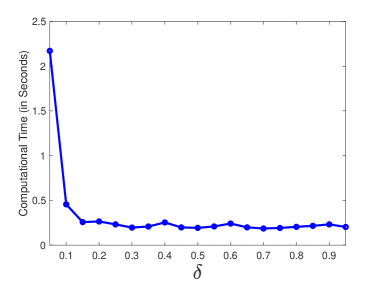
In Algorithm 1, there are two user chosen parameters. One is convergence parameter δ(0,1)𝛿01\delta\in(0,1) and the other one maxrun𝑚𝑎𝑥𝑟𝑢𝑛maxrun is the maximum number of iterations allowed. Following the suggestion by Fellman (1974) and Fiacco and Kortanek (1983), convergence parameter δ=12𝛿12\delta=\frac{1}{2} is usually used for A-optimality. Since EI-optimality has similar mathematical structure to A-optimality, we choose δ=12𝛿12\delta=\frac{1}{2} in our algorithm. It is also observed that the computational performance of the proposed algorithm is regarding δ𝛿\delta in Example 2 of Section 5. We will show later in proposition 1 that Algorithm 1 converges to optimal weights monotonically. Thus, the algorithm is not very sensitive to the choice of maximum iterations allowed, maxrun𝑚𝑎𝑥𝑟𝑢𝑛maxrun. In all our numerical examples, we choose maxrun=100𝑚𝑎𝑥𝑟𝑢𝑛100maxrun=100, while the same parameter in Yang et al. (2013) for Newton’s method is 40. The following theorem provides a sufficient condition when the iterative formula in Algorithm 1 is feasible, and Corollary 3 shows that, for EI-optimality, one can ensure that every iteration in Algorithm 1 is always feasible by choosing appropriate basis functions.

Theorem 2.

Suppose 𝖨(ξ𝛌k)1𝖡0𝖨superscriptsuperscript𝜉superscript𝛌𝑘1𝖡0{\mathsf{I}}(\xi^{\boldsymbol{\lambda}^{k}})^{-1}{\mathsf{B}}\neq 0 in iteration k𝑘k, then the iteration in equation (6) is feasible, i.e., the denominator

i=1nλik[w(𝒙i)𝒈(𝒙i)T𝖨(ξ𝝀k)1𝖡(𝖨(ξ𝝀k)1𝖡)p1𝖨(ξ𝝀k)1𝒈(𝒙i)]δsuperscriptsubscript𝑖1𝑛superscriptsubscript𝜆𝑖𝑘superscriptdelimited-[]𝑤subscript𝒙𝑖𝒈superscriptsubscript𝒙𝑖𝑇𝖨superscriptsuperscript𝜉superscript𝝀𝑘1𝖡superscript𝖨superscriptsuperscript𝜉superscript𝝀𝑘1𝖡𝑝1𝖨superscriptsuperscript𝜉superscript𝝀𝑘1𝒈subscript𝒙𝑖𝛿\sum\limits_{i=1}^{n}\lambda_{i}^{k}\left[w(\boldsymbol{x}_{i})\boldsymbol{g}(\boldsymbol{x}_{i})^{T}{\mathsf{I}}(\xi^{\boldsymbol{\lambda}^{k}})^{-1}{\mathsf{B}}\left({\mathsf{I}}(\xi^{\boldsymbol{\lambda}^{k}})^{-1}{\mathsf{B}}\right)^{p-1}{\mathsf{I}}(\xi^{\boldsymbol{\lambda}^{k}})^{-1}\boldsymbol{g}(\boldsymbol{x}_{i})\right]^{\delta}

is positive.

For the EI-optimality, the iterative formula in Algorithm 1 becomes

λik+1superscriptsubscript𝜆𝑖𝑘1\displaystyle\lambda_{i}^{k+1} =\displaystyle= λik[w(𝒙i)𝒈(𝒙i)T𝖨(ξ𝝀k)1𝖠𝖨(ξ𝝀k)1𝒈(𝒙i)]δi=1nλik[w(𝒙i)𝒈(𝒙i)T𝖨(ξ𝝀k)1𝖠𝖨(ξ𝝀k)1𝒈(𝒙i)]δ,superscriptsubscript𝜆𝑖𝑘superscriptdelimited-[]𝑤subscript𝒙𝑖𝒈superscriptsubscript𝒙𝑖𝑇𝖨superscriptsuperscript𝜉superscript𝝀𝑘1𝖠𝖨superscriptsuperscript𝜉superscript𝝀𝑘1𝒈subscript𝒙𝑖𝛿superscriptsubscript𝑖1𝑛superscriptsubscript𝜆𝑖𝑘superscriptdelimited-[]𝑤subscript𝒙𝑖𝒈superscriptsubscript𝒙𝑖𝑇𝖨superscriptsuperscript𝜉superscript𝝀𝑘1𝖠𝖨superscriptsuperscript𝜉superscript𝝀𝑘1𝒈subscript𝒙𝑖𝛿\displaystyle\lambda_{i}^{k}\frac{\left[w(\boldsymbol{x}_{i})\boldsymbol{g}(\boldsymbol{x}_{i})^{T}{\mathsf{I}}(\xi^{\boldsymbol{\lambda}^{k}})^{-1}{\mathsf{A}}{\mathsf{I}}(\xi^{\boldsymbol{\lambda}^{k}})^{-1}\boldsymbol{g}(\boldsymbol{x}_{i})\right]^{\delta}}{\sum\limits_{i=1}^{n}\lambda_{i}^{k}\left[w(\boldsymbol{x}_{i})\boldsymbol{g}(\boldsymbol{x}_{i})^{T}{\mathsf{I}}(\xi^{\boldsymbol{\lambda}^{k}})^{-1}{\mathsf{A}}{\mathsf{I}}(\xi^{\boldsymbol{\lambda}^{k}})^{-1}\boldsymbol{g}(\boldsymbol{x}_{i})\right]^{\delta}}, (7)

with 𝖠=Ω𝒈(𝒙)𝒈T(𝒙)[dh1dη]2dFIMSE(𝒙)𝖠subscriptΩ𝒈𝒙superscript𝒈𝑇𝒙superscriptdelimited-[]dsuperscript1d𝜂2differential-dsubscript𝐹IMSE𝒙{\mathsf{A}}=\int_{\Omega}\boldsymbol{g}(\boldsymbol{x})\boldsymbol{g}^{T}(\boldsymbol{x})\left[\frac{{\rm d}h^{-1}}{{\rm d}\eta}\right]^{2}{\rm d}F_{\operatorname{IMSE}}(\boldsymbol{x}).

Corollary 3.

For the EI-optimality, a positive definite 𝖠=Ω𝐠(𝐱)𝐠T(𝐱)[dh1dη]2dFIMSE(𝐱)𝖠subscriptΩ𝐠𝐱superscript𝐠𝑇𝐱superscriptdelimited-[]dsuperscript1d𝜂2differential-dsubscript𝐹IMSE𝐱{\mathsf{A}}=\int_{\Omega}\boldsymbol{g}(\boldsymbol{x})\boldsymbol{g}^{T}(\boldsymbol{x})\left[\frac{{\rm d}h^{-1}}{{\rm d}\eta}\right]^{2}{\rm d}F_{\operatorname{IMSE}}(\boldsymbol{x}) would ensure all the iterations in equation (6) to be always feasible, i.e., the denominator

i=1nλik[w(𝒙i)𝒈T(𝒙i)𝖨(ξ𝝀k)1𝖠𝖨(ξ𝝀k)1𝒈(𝒙i)]δsuperscriptsubscript𝑖1𝑛superscriptsubscript𝜆𝑖𝑘superscriptdelimited-[]𝑤subscript𝒙𝑖superscript𝒈𝑇subscript𝒙𝑖𝖨superscriptsuperscript𝜉superscript𝝀𝑘1𝖠𝖨superscriptsuperscript𝜉superscript𝝀𝑘1𝒈subscript𝒙𝑖𝛿\sum\limits_{i=1}^{n}\lambda_{i}^{k}\left[w(\boldsymbol{x}_{i})\boldsymbol{g}^{T}(\boldsymbol{x}_{i}){\mathsf{I}}(\xi^{\boldsymbol{\lambda}^{k}})^{-1}{\mathsf{A}}{\mathsf{I}}(\xi^{\boldsymbol{\lambda}^{k}})^{-1}\boldsymbol{g}(\boldsymbol{x}_{i})\right]^{\delta}

is always positive.

For the ΦpsubscriptΦ𝑝\Phi_{p}-optimality, the matrix 𝖡=(𝒇(𝜷)𝜷T)T(𝒇(𝜷)𝜷T)𝖡superscript𝒇𝜷superscript𝜷𝑇𝑇𝒇𝜷superscript𝜷𝑇{\mathsf{B}}=\left(\frac{\partial\boldsymbol{f}(\boldsymbol{\beta})}{\partial\boldsymbol{\beta}^{T}}\right)^{T}\left(\frac{\partial\boldsymbol{f}(\boldsymbol{\beta})}{\partial\boldsymbol{\beta}^{T}}\right) is determined by 𝒇(𝜷)𝒇𝜷\boldsymbol{f}(\boldsymbol{\beta}), the functions of 𝜷𝜷\boldsymbol{\beta} that are of interest, which are determined by the purpose of the experiment. But, for EI-optimality, the matrix 𝖠=Ω𝒈(𝒙)𝒈T(𝒙)[dh1dη]2dFIMSE(𝒙)𝖠subscriptΩ𝒈𝒙superscript𝒈𝑇𝒙superscriptdelimited-[]dsuperscript1d𝜂2differential-dsubscript𝐹IMSE𝒙{\mathsf{A}}=\int_{\Omega}\boldsymbol{g}(\boldsymbol{x})\boldsymbol{g}^{T}(\boldsymbol{x})\left[\frac{{\rm d}h^{-1}}{{\rm d}\eta}\right]^{2}{\rm d}F_{\operatorname{IMSE}}(\boldsymbol{x}) is always positive semi-definite and pre-determined before the optimal design is constructed. When a singular 𝖠𝖠{\mathsf{A}} is observed in the first step, one can choose the basis functions g1,,glsubscript𝑔1subscript𝑔𝑙g_{1},...,g_{l} carefully so that they are (nearly) orthogonal functions such that

Ωgi(𝒙)gj(𝒙)[dh1dη]2dFIMSE(𝒙)0forij.subscriptΩsubscript𝑔𝑖𝒙subscript𝑔𝑗𝒙superscriptdelimited-[]dsuperscript1d𝜂2differential-dsubscript𝐹IMSE𝒙0for𝑖𝑗\int_{\Omega}g_{i}(\boldsymbol{x})g_{j}(\boldsymbol{x})\left[\frac{{\rm d}h^{-1}}{{\rm d}\eta}\right]^{2}{\rm d}F_{\operatorname{IMSE}}(\boldsymbol{x})\approx 0\,\,\,\,\text{for}\,\,\,\,i\neq j.

By doing this, one can ensure the matrix 𝖠𝖠{\mathsf{A}} to be positive definite. In general, the Gram-Schmidt orthogonalization (Pursell and Trimble 1991) can be used to construct uni/multi-variate orthogonal basis functions.

We can provide the convergence property of Algorithm 1, which generalizes Yu’s work (Yu 2010) to a broader class of optimality criteria, ΦpsubscriptΦ𝑝\Phi_{p}-optimality.

Proposition 1 (Convergence of Algorithm 1).

Given the design points 𝐱1,,𝐱nsubscript𝐱1subscript𝐱𝑛\boldsymbol{x}_{1},...,\boldsymbol{x}_{n} fixed, the weight vector 𝛌ksuperscript𝛌𝑘\boldsymbol{\lambda}^{k} obtained from Algorithm 1 monotonically converges to the optimal weight vector 𝛌superscript𝛌\boldsymbol{\lambda}^{*} that minimizes ΦpsubscriptΦ𝑝\Phi_{p}-optimality, as k𝑘k\rightarrow\infty.

4 Proposed Sequential Algorithm of Constructing EI-Optimal Design

In this section, we will describe the proposed efficient algorithm for constructing EI-optimal design for GLMs. General equivalence theorem is one of the main theoretical tools to develop algorithms to construct optimal designs. Many Wynn-Federov type algorithms are developed based on general equivalence theorem (See Wynn 1970, 1972; Whittle 1973; Yang et al. 2013; Martín and Gutiérrez 2015). Yang et al. (2016) developed an efficient algorithm to construct 2ksuperscript2𝑘2^{k} D-optimal factorial design with binary response based on a specialized version of general equivalence theorem on a pre-determined finite set of design points. We will first establish the general equivalence theorem for EI-optimality of GLMs in Section 4.1, which provides an intuitive way for choosing the support points to construct an EI-optimal design in a sequential fashion. Section 4.2 details the proposed algorithm and develops the convergence property of the proposed algorithm.

4.1 General Equivalence Theorem of EI-Optimality

As shown in Remark 1, the EI-optimality has a similar mathematical structure as the Φ1subscriptΦ1\Phi_{1}-optimatliy, but the two criteria have different practical interpretations. The General Equivalence Theorem of ΦpsubscriptΦ𝑝\Phi_{p}-optimality for generalized linear models has been established (Stufken and Yang 2011), and it could be extended to EI-optimality for GLMs easily. We state the General Equivalence Theorem of EI-optimality for GLMs in the following Theorem 3, and the standard proof is omitted. The extended theoretical results facilitate the sequential choice of support points as that of Fedorov-Wynn algorithm (Wynn 1970; Fedorov 1972).

Given two designs ξ𝜉\xi and ξsuperscript𝜉\xi^{\prime}, let the design ξ~~𝜉\tilde{\xi} be constructed as

ξ~=(1α)ξ+αξ.~𝜉1𝛼𝜉𝛼superscript𝜉\tilde{\xi}=(1-\alpha)\xi+\alpha\xi^{\prime}.

Then, the derivative of EI(ξ,𝜷,FIMSE)EI𝜉𝜷subscript𝐹IMSE\text{EI}(\xi,\boldsymbol{\beta},F_{\operatorname{IMSE}}) in the direction of design ξsuperscript𝜉\xi^{\prime} is

ϕ(ξ,ξ)=limα0+EI(ξ~,𝜷,FIMSE)EI(ξ,𝜷,FIMSE)α.italic-ϕsuperscript𝜉𝜉subscript𝛼superscript0EI~𝜉𝜷subscript𝐹IMSEEI𝜉𝜷subscript𝐹IMSE𝛼\phi(\xi^{\prime},\xi)=\lim\limits_{\alpha\rightarrow 0^{+}}\frac{\text{EI}(\tilde{\xi},\boldsymbol{\beta},F_{\operatorname{IMSE}})-\text{EI}(\xi,\boldsymbol{\beta},F_{\operatorname{IMSE}})}{\alpha}. (8)
Lemma 4.

The EI(,𝛃,FIMSE)EI𝛃subscript𝐹IMSE\text{EI}(\cdot,\boldsymbol{\beta},F_{\operatorname{IMSE}}) is a convex function of the design ξ𝜉\xi.

With some algebra, we can obtain the directional derivative of EI(ξ,𝜷,Ωc)𝐸𝐼𝜉𝜷subscriptΩ𝑐EI(\xi,\boldsymbol{\beta},\Omega_{c}) in the direction of any design ξsuperscript𝜉\xi^{\prime} as,

ϕ(ξ,ξ)=limα0+EI(ξ~,𝜷,FIMSE)EI(ξ,𝜷,FIMSE)α=tr(𝖨(ξ)1𝖠)tr(𝖨(ξ)𝖨(ξ)1𝖠𝖨(ξ)1),italic-ϕsuperscript𝜉𝜉subscript𝛼superscript0EI~𝜉𝜷subscript𝐹IMSEEI𝜉𝜷subscript𝐹IMSE𝛼tr𝖨superscript𝜉1𝖠tr𝖨superscript𝜉𝖨superscript𝜉1𝖠𝖨superscript𝜉1\phi(\xi^{\prime},\xi)=\lim\limits_{\alpha\rightarrow 0^{+}}\frac{\text{EI}(\tilde{\xi},\boldsymbol{\beta},F_{\operatorname{IMSE}})-\text{EI}(\xi,\boldsymbol{\beta},F_{\operatorname{IMSE}})}{\alpha}=\operatorname{tr}({\mathsf{I}}(\xi)^{-1}{\mathsf{A}})-\operatorname{tr}({\mathsf{I}}(\xi^{\prime}){\mathsf{I}}(\xi)^{-1}{\mathsf{A}}{\mathsf{I}}(\xi)^{-1}),

where 𝖠=Ω𝒈(𝒙)𝒈T(𝒙)[dh1dη]2dFIMSE(𝒙)𝖠subscriptΩ𝒈𝒙superscript𝒈𝑇𝒙superscriptdelimited-[]dsuperscript1d𝜂2differential-dsubscript𝐹IMSE𝒙{\mathsf{A}}=\int_{\Omega}\boldsymbol{g}(\boldsymbol{x})\boldsymbol{g}^{T}(\boldsymbol{x})\left[\frac{{\rm d}h^{-1}}{{\rm d}\eta}\right]^{2}{\rm d}F_{\operatorname{IMSE}}(\boldsymbol{x}). Moreover, we can also get the directional derivative of EI(ξ,𝜷,FIMSE)EI𝜉𝜷subscript𝐹IMSE\text{EI}(\xi,\boldsymbol{\beta},F_{\operatorname{IMSE}}) in the direction of a single point 𝒙𝒙\boldsymbol{x} as,

ϕ(𝒙,ξ)=tr(𝖨(ξ)1𝖠)w(𝒙)𝒈(𝒙)T𝖨(ξ)1𝖠𝖨(ξ)1𝒈(𝒙).italic-ϕ𝒙𝜉tr𝖨superscript𝜉1𝖠𝑤𝒙𝒈superscript𝒙𝑇𝖨superscript𝜉1𝖠𝖨superscript𝜉1𝒈𝒙\phi(\boldsymbol{x},\xi)=\operatorname{tr}({\mathsf{I}}(\xi)^{-1}{\mathsf{A}})-w(\boldsymbol{x})\boldsymbol{g}(\boldsymbol{x})^{T}{\mathsf{I}}(\xi)^{-1}{\mathsf{A}}{\mathsf{I}}(\xi)^{-1}\boldsymbol{g}(\boldsymbol{x}).
Theorem 3 (General Equivalence Theorem).

The following three conditions of ξsuperscript𝜉\xi^{*} are equivalent:

  1. 1.

    The design ξsuperscript𝜉\xi^{*} minimizes

    EI(ξ,𝜷,Ωc)=tr(𝖠𝖨(ξ)1).EI𝜉𝜷subscriptΩ𝑐tr𝖠𝖨superscript𝜉1\text{EI}(\xi,\boldsymbol{\beta},\Omega_{c})=\operatorname{tr}({\mathsf{A}}{\mathsf{I}}(\xi)^{-1}).
  2. 2.

    The design ξsuperscript𝜉\xi^{*} minimizes

    sup𝒙Ωw(𝒙)𝒈T(𝒙)𝖨(ξ)1𝖠𝖨(ξ)1𝒈(𝒙).subscriptsupremum𝒙Ω𝑤𝒙superscript𝒈𝑇𝒙𝖨superscript𝜉1𝖠𝖨superscript𝜉1𝒈𝒙\sup\limits_{\boldsymbol{x}\in\Omega}w(\boldsymbol{x})\boldsymbol{g}^{T}(\boldsymbol{x}){\mathsf{I}}(\xi)^{-1}{\mathsf{A}}{\mathsf{I}}(\xi)^{-1}\boldsymbol{g}(\boldsymbol{x}).
  3. 3.

    w(𝒙)𝒈T(𝒙)𝖨(ξ)1𝖠𝖨(ξ)1𝒈(𝒙)tr(𝖨(ξ)1𝖠)𝑤𝒙superscript𝒈𝑇𝒙𝖨superscriptsuperscript𝜉1𝖠𝖨superscriptsuperscript𝜉1𝒈𝒙tr𝖨superscriptsuperscript𝜉1𝖠w(\boldsymbol{x})\boldsymbol{g}^{T}(\boldsymbol{x}){\mathsf{I}}(\xi^{*})^{-1}{\mathsf{A}}{\mathsf{I}}(\xi^{*})^{-1}\boldsymbol{g}(\boldsymbol{x})\leq\operatorname{tr}({\mathsf{I}}(\xi^{*})^{-1}{\mathsf{A}}) holds over the experimental region ΩΩ\Omega, and the equality holds only at the points of support of the design ξsuperscript𝜉\xi^{*}.

According to Theorem 3, for an optimal design ξsuperscript𝜉\xi^{*}, the directional derivative ϕ(𝒙,ξ)italic-ϕ𝒙superscript𝜉\phi(\boldsymbol{x},\xi^{*}) is non-negative for any 𝒙Ω𝒙Ω\boldsymbol{x}\in\Omega. It implies that for any non-optimal design, there will be some directions in which the directional derivative ϕ(𝒙,ξ)<0italic-ϕ𝒙𝜉0\phi(\boldsymbol{x},\xi)<0. Given a current design ξ𝜉\xi, to gain the maximal decrease in the EI-optimality criterion, we would choose a new support point 𝒙superscript𝒙\boldsymbol{x}^{*} to be added into the design, if ϕ(𝒙,ξ)=min𝒙Ωϕ(𝒙,ξ)<0italic-ϕsuperscript𝒙𝜉subscript𝒙Ωitalic-ϕ𝒙𝜉0\phi(\boldsymbol{x}^{*},\xi)=\min\limits_{\boldsymbol{x}\in\Omega}\phi(\boldsymbol{x},\xi)<0. Then one can optimize the weights of all support points in the updated design, which is described in Algorithm 1 in Section 3. With this greedy search of the design points, we hope that most/all optimal weights in each iteration are nonzero, and the multiplicative algorithm converges quickly. By iterating the selection of support point and the weight update of all support points, this two-step iterative procedure can be continued until min𝒙Ωϕ(𝒙,ξ)0subscript𝒙Ωitalic-ϕ𝒙𝜉0\min\limits_{\boldsymbol{x}\in\Omega}\phi(\boldsymbol{x},\xi)\geq 0 for all 𝒙Ω𝒙Ω\boldsymbol{x}\in\Omega, which means the updated design is EI-optimal. Such a sequential algorithm of constructing optimal designs, as described in Algorithm 2 in Section 4.2, follows similar spirits in the widely-used Fedorov-Wynn algorithm (Wynn 1970;Wynn 1972), the multi-stage algorithm proposed by Yang et al. (2013), and the combined algorithm proposed by Martín and Gutiérrez (2015). It is worth pointing out that when the region of explanatory variable 𝒙𝒙\boldsymbol{x} we are interested in, ΩCsubscriptΩ𝐶\Omega_{C} is a subset of original experimental region ΩΩ\Omega, the optimal design ξsuperscript𝜉\xi^{*} is still defined and searched on the original experimental region ΩΩ\Omega. As a result, the support points in the optimal design may locate outside ΩCsubscriptΩ𝐶\Omega_{C}.

4.2 The Proposed Sequential Algorithm

As discussed in Section 3.2, the multiplicative algorithm tends to converge slowly under a large candidate set. The theoretical results in Theorem 3 provide insightful guidelines on sequential selection of design points. In combination with Algorithm 1 to find optimal weights for fixed design points in Section 3, we propose an efficient sequential algorithm to construct the EI-optimal design for generalized linear models. The details of the proposed sequential algorithm is summarized in Algorithm 2.

Algorithm 2
1:Calculate matrix 𝖠=Ω𝒈(𝒙)𝒈T(𝒙)[dh1dη]2dFIMSE(𝒙)𝖠subscriptΩ𝒈𝒙superscript𝒈𝑇𝒙superscriptdelimited-[]dsuperscript1d𝜂2differential-dsubscript𝐹IMSE𝒙{\mathsf{A}}=\int_{\Omega}\boldsymbol{g}(\boldsymbol{x})\boldsymbol{g}^{T}(\boldsymbol{x})\left[\frac{{\rm d}h^{-1}}{{\rm d}\eta}\right]^{2}{\rm d}F_{\operatorname{IMSE}}(\boldsymbol{x}).
2:if cond(𝖠>1e16𝖠1𝑒16{\mathsf{A}}>1e16then
3:     Construct orthogonal basis 𝒈𝒈\boldsymbol{g} using Gram-Schmidt orthogonalization.
4:     Calculate matrix 𝖠𝖠{\mathsf{A}} using the new orthogonal basis 𝒈𝒈\boldsymbol{g}.
5:end if
6:Generate an N𝑁N points candidate pool 𝒞𝒞\mathcal{C} using grid or Sobol sequence from experimental region ΩΩ\Omega.
7:Choose an initial design points set 𝒳0={𝒙1,,𝒙l+1}superscript𝒳0subscript𝒙1subscript𝒙𝑙1\mathcal{X}^{0}=\left\{\boldsymbol{x}_{1},\cdots,\boldsymbol{x}_{l+1}\right\} containing l+1𝑙1l+1 points.
8:Obtain optimal weights 𝝀0superscript𝝀0\boldsymbol{\lambda}^{0} of initial design points set 𝒳0superscript𝒳0\mathcal{X}^{0} using Algorithm 1 and form the initial design ξ0={𝒳0𝝀0}superscript𝜉0superscript𝒳0missing-subexpressionsuperscript𝝀0missing-subexpression\xi^{0}=\left\{\begin{array}[]{cc}\mathcal{X}^{0}\\ \boldsymbol{\lambda}^{0}\end{array}\right\}.
9:Calculate the lower bound of EI-efficiency of ξ0superscript𝜉0\xi^{0},
LEff(ξ0|ξ)=tr(𝖨1(ξ0)𝖠)max𝒙𝒞w(𝒙)𝒈(𝒙)T𝖨(ξ0)1𝖠𝖨(ξ0)1𝒈(𝒙).LEffconditionalsuperscript𝜉0superscript𝜉trsuperscript𝖨1superscript𝜉0𝖠subscript𝒙𝒞𝑤𝒙𝒈superscript𝒙𝑇𝖨superscriptsuperscript𝜉01𝖠𝖨superscriptsuperscript𝜉01𝒈𝒙\operatorname{LEff}(\xi^{0}|\xi^{*})=\frac{\operatorname{tr}({\mathsf{I}}^{-1}(\xi^{0}){\mathsf{A}})}{\max\limits_{\boldsymbol{x}\in\mathcal{C}}w(\boldsymbol{x})\boldsymbol{g}(\boldsymbol{x})^{T}{\mathsf{I}}(\xi^{0})^{-1}{\mathsf{A}}{\mathsf{I}}(\xi^{0})^{-1}\boldsymbol{g}(\boldsymbol{x})}.
10:Set r=1𝑟1r=1.
11:while LEffEI(ξr1|ξ)<reqeffsubscriptLEffEIconditionalsuperscript𝜉𝑟1superscript𝜉𝑟𝑒𝑞𝑒𝑓𝑓\operatorname{LEff}_{\text{EI}}(\xi^{r-1}|\xi^{*})<reqeff and r<maxiter𝑟𝑚𝑎𝑥𝑖𝑡𝑒𝑟r<maxiter do
12:     Add the point 𝒙r=argmin𝒙𝒞ϕ(𝒙,ξr1)superscriptsubscript𝒙𝑟subscriptargmin𝒙𝒞italic-ϕ𝒙superscript𝜉𝑟1\boldsymbol{x}_{r}^{*}=\operatorname*{argmin}\limits_{\boldsymbol{x}\in\mathcal{C}}\phi(\boldsymbol{x},\xi^{r-1}) to the current design points set, i.e., 𝒳r=𝒳r1𝒙rsuperscript𝒳𝑟superscript𝒳𝑟1superscriptsubscript𝒙𝑟\mathcal{X}^{r}=\mathcal{X}^{r-1}\cup\boldsymbol{x}_{r}^{*}, where ϕ(𝒙,ξr1)italic-ϕ𝒙superscript𝜉𝑟1\phi(\boldsymbol{x},\xi^{r-1}) is the directional derivative expressed as
ϕ(𝒙,ξr1)=tr(𝖨(ξr1)1𝖠)w(𝒙)𝒈(𝒙)T𝖨(ξr1)1𝖠𝖨(ξr1)1𝒈(𝒙).italic-ϕ𝒙superscript𝜉𝑟1tr𝖨superscriptsuperscript𝜉𝑟11𝖠𝑤𝒙𝒈superscript𝒙𝑇𝖨superscriptsuperscript𝜉𝑟11𝖠𝖨superscriptsuperscript𝜉𝑟11𝒈𝒙\phi(\boldsymbol{x},\xi^{r-1})=\operatorname{tr}({\mathsf{I}}(\xi^{r-1})^{-1}{\mathsf{A}})-w(\boldsymbol{x})\boldsymbol{g}(\boldsymbol{x})^{T}{\mathsf{I}}(\xi^{r-1})^{-1}{\mathsf{A}}{\mathsf{I}}(\xi^{r-1})^{-1}\boldsymbol{g}(\boldsymbol{x}).
13:     Obtain optimal weights 𝝀rsuperscript𝝀𝑟\boldsymbol{\lambda}^{r} of the current design points set 𝒳rsuperscript𝒳𝑟\mathcal{X}^{r} using Algorithm 1 and form the current design ξr={𝒳r𝝀r}superscript𝜉𝑟superscript𝒳𝑟missing-subexpressionsuperscript𝝀𝑟missing-subexpression\xi^{r}=\left\{\begin{array}[]{cc}\mathcal{X}^{r}\\ \boldsymbol{\lambda}^{r}\end{array}\right\}.
14:     Calculate the lower bound of EI-efficiency of ξrsuperscript𝜉𝑟\xi^{r},
LEffEI(ξr|ξ)=tr(𝖨1(ξr)𝖠)max𝒙𝒞w(𝒙)𝒈(𝒙)T𝖨(ξr)1𝖠𝖨(ξr)1𝒈(𝒙).subscriptLEffEIconditionalsuperscript𝜉𝑟superscript𝜉trsuperscript𝖨1superscript𝜉𝑟𝖠subscript𝒙𝒞𝑤𝒙𝒈superscript𝒙𝑇𝖨superscriptsuperscript𝜉𝑟1𝖠𝖨superscriptsuperscript𝜉𝑟1𝒈𝒙\operatorname{LEff}_{\text{EI}}(\xi^{r}|\xi^{*})=\frac{\operatorname{tr}({\mathsf{I}}^{-1}(\xi^{r}){\mathsf{A}})}{\max\limits_{\boldsymbol{x}\in\mathcal{C}}w(\boldsymbol{x})\boldsymbol{g}(\boldsymbol{x})^{T}{\mathsf{I}}(\xi^{r})^{-1}{\mathsf{A}}{\mathsf{I}}(\xi^{r})^{-1}\boldsymbol{g}(\boldsymbol{x})}.
15:     r=r+1𝑟𝑟1r=r+1.
16:end while

The efficiency of a design ξ𝜉\xi relative to another design ξsuperscript𝜉\xi^{\prime} under a ΦpsubscriptΦ𝑝\Phi_{p}-optimality is defined as (Pukelsheim 2006)

EffΦp(ξ|ξ)=Φp(ξ)Φp(ξ).subscriptEffsubscriptΦ𝑝conditional𝜉superscript𝜉subscriptΦ𝑝superscript𝜉subscriptΦ𝑝𝜉\operatorname{Eff}_{\Phi_{p}}(\xi|\xi^{\prime})=\frac{\Phi_{p}(\xi^{\prime})}{\Phi_{p}(\xi)}.

Asymptotically, the efficiency is essentially the ratio between the number of trials required to obtain the same amount of information measured by a specific ΦpsubscriptΦ𝑝\Phi_{p}-optimality using design ξsuperscript𝜉\xi^{\prime} and ξ𝜉\xi. The following proposition provides a lower bound LEffΦp(ξ|ξ)subscriptLEffsubscriptΦ𝑝conditional𝜉superscript𝜉\operatorname{LEff}_{\Phi_{p}}(\xi|\xi^{*}) of ΦpsubscriptΦ𝑝\Phi_{p}-efficiency of a design ξ𝜉\xi relative to the corresponding ΦpsubscriptΦ𝑝\Phi_{p}-optimal design ξsuperscript𝜉\xi^{*}, and this lower bound is used in the stopping rule in Algorithm 2.

Theorem 4.

With candidate pool 𝒞𝒞\mathcal{C}, the ΦpsubscriptΦ𝑝\Phi_{p}-efficiency of any design ξ𝜉\xi relative to ΦpsubscriptΦ𝑝\Phi_{p}-optimal design ξsuperscript𝜉\xi^{*}, EffΦp(ξ|ξ)subscriptEffsubscriptΦ𝑝conditional𝜉superscript𝜉\operatorname{Eff}_{\Phi_{p}}(\xi|\xi^{*}), is lower bounded by

LEffΦp(ξ|ξ)=Φp(ξ)max𝒙𝒞q1/p[tr(𝖨(ξ)1𝖡)p]1/p1w(𝒙i)𝒈(𝒙i)T𝖨(ξ)1𝖡(𝖨(ξ)1𝖡)p1𝖨(ξ)1𝒈(𝒙i).\displaystyle\operatorname{LEff}_{\Phi_{p}}(\xi|\xi^{*})=\frac{\Phi_{p}(\xi)}{\max\limits_{\boldsymbol{x}\in\mathcal{C}}q^{-1/p}\left[\operatorname{tr}\left({\mathsf{I}}(\xi)^{-1}{\mathsf{B}}\right)^{p}\right]^{1/p-1}w(\boldsymbol{x}_{i})\boldsymbol{g}(\boldsymbol{x}_{i})^{T}{\mathsf{I}}(\xi)^{-1}{\mathsf{B}}\left({\mathsf{I}}(\xi)^{-1}{\mathsf{B}}\right)^{p-1}{\mathsf{I}}(\xi)^{-1}\boldsymbol{g}(\boldsymbol{x}_{i})}. (9)

Specifically, for EI-optimality, the lower bound of a design ξ𝜉\xi relative to the corresponding EI-optimal design ξsuperscript𝜉\xi^{*} is

LEffEI(ξ|ξ)=tr(𝖨1(ξ)𝖠)max𝒙𝒞w(𝒙)𝒈(𝒙)T𝖨(ξ)1𝖠𝖨(ξ)1𝒈(𝒙).subscriptLEffEIconditional𝜉superscript𝜉trsuperscript𝖨1𝜉𝖠subscript𝒙𝒞𝑤𝒙𝒈superscript𝒙𝑇𝖨superscript𝜉1𝖠𝖨superscript𝜉1𝒈𝒙\operatorname{LEff}_{\text{EI}}(\xi|\xi^{*})=\frac{\operatorname{tr}({\mathsf{I}}^{-1}(\xi){\mathsf{A}})}{\max\limits_{\boldsymbol{x}\in\mathcal{C}}w(\boldsymbol{x})\boldsymbol{g}(\boldsymbol{x})^{T}{\mathsf{I}}(\xi)^{-1}{\mathsf{A}}{\mathsf{I}}(\xi)^{-1}\boldsymbol{g}(\boldsymbol{x})}.

Following the stopping criterion used in (Harman et al. 2019), when the lower bound LEffEI(ξr|ξ)subscriptLEffEIconditionalsuperscript𝜉𝑟superscript𝜉\operatorname{LEff}_{\text{EI}}(\xi^{r}|\xi^{*}) of the efficiency EffEI(ξr|ξ)subscriptEffEIconditionalsuperscript𝜉𝑟superscript𝜉\operatorname{Eff}_{\text{EI}}(\xi^{r}|\xi^{*}) reaches a user specified threshold reqeff𝑟𝑒𝑞𝑒𝑓𝑓reqeff, there is no practical reason to continue the search. We choose reqeff=0.99𝑟𝑒𝑞𝑒𝑓𝑓0.99reqeff=0.99 in all the numerical examples. Another user specified parameter is the maximum iterations allowed, maxiter𝑚𝑎𝑥𝑖𝑡𝑒𝑟maxiter. We choose maxiter=100𝑚𝑎𝑥𝑖𝑡𝑒𝑟100maxiter=100, and the proposed algorithm converges within 100 iterations in all the numerical examples conducted, while Newton’s method fails to converge within 100 iterations for one case in Example 2. More details could be found in Section 5.

Note that the proposed sequential algorithm of constructing EI-optimal design for GLMs does not require the computation of Hessian matrix inversion as in Newton-Raphson methods. Thus it can avoid issue of singular Hessian matrix and can be computationally efficient than the conventional methods. The sequential nature of the proposed algorithm also enables efficient search of optimal weights without updating weights for all candidates points. Martín and Gutiérrez (2015) considered a similar sequential algorithm that combines Whittle’s method (Whittle 1973) with one iteration of multiplicative algorithm to update the weights after a new design point is added. As a result, the weights are not necessarily optimized in each iteration of the combined algorithm, and the proof of Theorem 5 can not be applied to the combined algorithm. The convergence property of the combined algorithm for general ΦpsubscriptΦ𝑝\Phi_{p}-optimality is not studied in Martín and Gutiérrez (2015).

Note that the sequential algorithm (Algorithm 2) can also be easily modified to achieve ϕpsubscriptitalic-ϕ𝑝\phi_{p}-optimal designs, where the analytic formula of directional derivative ϕ(𝒙,ξ)italic-ϕ𝒙𝜉\phi(\boldsymbol{x},\xi) for ϕpsubscriptitalic-ϕ𝑝\phi_{p}-optimality has been studied in several existing literature (Atkinson et al. 2006; Stufken and Yang 2011; Yang et al. 2013, etc.). Moreover, we also establish the convergence property of the proposed sequential algorithm as follows.

Theorem 5 (Convergence of Algorithm 2).

With a discrete design region 𝒞𝒞\mathcal{C}, the design constructed by Algorithm 2 converges to EI-optimal design ξsuperscript𝜉\xi^{*} that minimizes EI(ξ,𝛃,FIMSE)𝐸𝐼𝜉𝛃subscript𝐹IMSEEI(\xi,\boldsymbol{\beta},F_{\operatorname{IMSE}}), as r𝑟r\rightarrow\infty, i.e.,

limrEI(ξr,𝜷,FIMSE)=EI(ξ,𝜷,FIMSE).subscript𝑟EIsuperscript𝜉𝑟𝜷subscript𝐹IMSEEIsuperscript𝜉𝜷subscript𝐹IMSE\lim\limits_{r\rightarrow\infty}\text{EI}(\xi^{r},\boldsymbol{\beta},F_{\operatorname{IMSE}})=\text{EI}(\xi^{*},\boldsymbol{\beta},F_{\operatorname{IMSE}}).

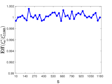
When the experimental region ΩΩ\Omega is continuous, a discretization would be needed to form the candidate pool 𝒞𝒞\mathcal{C}. We would like to point out that the choice of candidate pool 𝒞𝒞\mathcal{C} would affect the efficiency of Algorithm 2, and the computational time increases dramatically as the candidate pool gets large. We suggest using grid as the candidate pool when the dimension of explanatory variables is small, and choosing the Sobol sequence (Sobol 1967) as the candidate pool when the explanatory variable dimension is large. The Sobol sequence is a space-filling design that covers the experimental domain ΩΩ\Omega well and is efficient when the dimension of the explanatory variable is high. To further improve the efficiency of the algorithm, a search strategy inspired by Yang and Stufken (2012) could be employed. One can start with a more sparse Sobol sequence, and achieve the current best design using Algorithm 2. Then, we can further create denser and denser candidate pool in the neighborhood of the support points in the current best design until there is no further improvement under the EI-optimality criterion.

5 Numerical Examples

In this section, we will conduct numerical studies to evaluate the performance of the proposed sequential algorithm (Algorithm 2). As noted in Section 4.2, Algorithm 2 can be applied to construct ΦpsubscriptΦ𝑝\Phi_{p}-optimal designs such as A-optimal design. Based on our best knowledge, there is no existing algorithm that can directly construct the EI-optimal design for GLMs. However, the Newton-type method (Yang et al. 2013) could be revised to construct EI-optimal design. The proposed algorithm (Algorithm 2) will be compared with the Newton-type method in Yang et al. (2013), which adopts Newton’s method to update the weights of design points and is an efficient algorithm in the literature. The comparison will be conducted under different generalized linear models with various settings of variable dimensions. Both algorithms are implemented in Matlab, and the code for Newton’s method is converted from the SAS code kindly provided by the authors of Yang et al. (2013). All codes were run on a MacBook Pro with 2.4 GHz Intel Core i5 processor. The Newton-type method requires a well-conditioned Hessian matrix to update the weights, but the Hessian matrix could be numerically singular in a certain iteration and results in inaccurate weight updates. In this numerical example, the generalized inverse of Hessian matrix is used for the Newton-type method. The proposed algorithm always returns nonnegative weights, only eliminates the design points with almost zero weight and does not require Hessian matrix inversion. Grid candidate pool of size N=(s+1)d𝑁superscript𝑠1𝑑N=(s+1)^{d} with s+1𝑠1s+1 equally spaced points for each explanatory variable xisubscript𝑥𝑖x_{i}, i=1,,d𝑖1𝑑i=1,\cdots,d is used in all numerical examples. Note that our Algorithm 2 does not require the candidate pool to be a grid. We would suggest using space-filling design such as Sobol sequence as the candidate pool for high-dimensional explanatory variable. The target efficiency lower bound reqeff𝑟𝑒𝑞𝑒𝑓𝑓reqeff in the stopping criterion is chosen to be 0.99, and we consider two designs are both good enough if their efficiency lower bounds exceed 0.99. Thus, it is fair to compare the efficiency of the algorithms based on the computational time.

Example 1. The setting of this example follows the Example 2 in (Yang et al. 2013), which considers the linear model

Y𝑌\displaystyle Y similar-to\displaystyle\sim θ1+θ2x1+θ3x12+θ4x2+θ5x1x2+N(0,σ2),subscript𝜃1subscript𝜃2subscript𝑥1subscript𝜃3superscriptsubscript𝑥12subscript𝜃4subscript𝑥2subscript𝜃5subscript𝑥1subscript𝑥2𝑁0superscript𝜎2\displaystyle\theta_{1}+\theta_{2}x_{1}+\theta_{3}x_{1}^{2}+\theta_{4}x_{2}+\theta_{5}x_{1}x_{2}+N(0,\sigma^{2}),
𝜽𝜽\displaystyle\boldsymbol{\theta} =\displaystyle= (θ1,θ2,θ3,θ4,θ5),subscript𝜃1subscript𝜃2subscript𝜃3subscript𝜃4subscript𝜃5\displaystyle(\theta_{1},\theta_{2},\theta_{3},\theta_{4},\theta_{5}),

where Ω={(2i/s1,j/s)}Ω2𝑖𝑠1𝑗𝑠\Omega=\{(2i/s-1,j/s)\}, i=0,1,,s,j=0,1,,s}i=0,1,...,s,j=0,1,...,s\}, where s𝑠s is the number of grid points in each variable and the total number of points in ΩΩ\Omega is N=(s+1)2𝑁superscript𝑠12N=(s+1)^{2}. Note that since the experimental region is discrete, it is not necessary to discretize the experimental region. The proposed algorithm and the Newton-type method are compared under A- and EI-optimality. For EI-optimality, we choose FIMSE=Funifsubscript𝐹IMSEsubscript𝐹unifF_{\operatorname{IMSE}}=F_{\text{\rm unif}}.

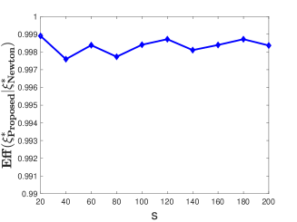
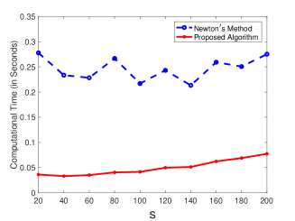
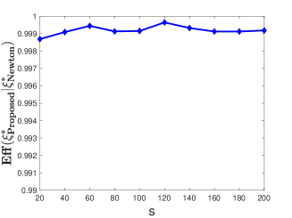
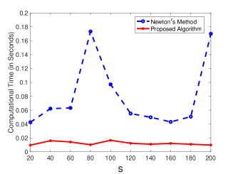
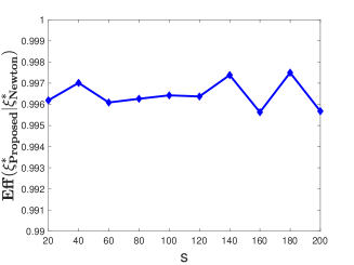
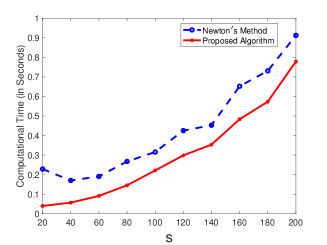
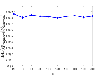
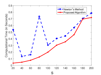
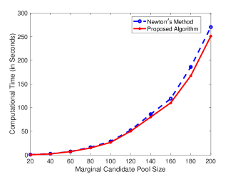
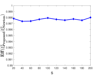
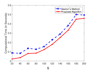
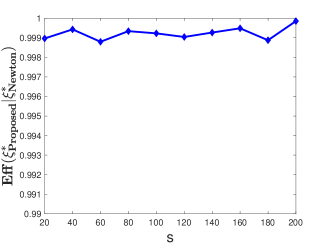
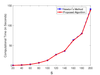
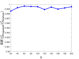
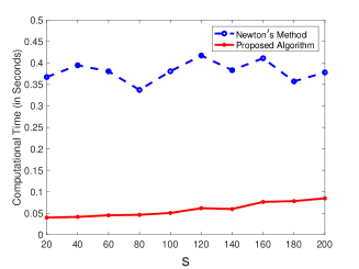
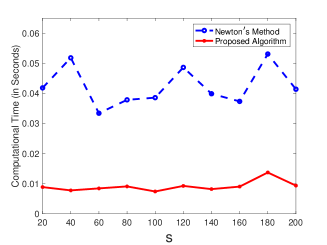
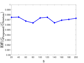
Here we consider the same initial design, consisting of five randomly chosen points in ΩΩ\Omega, for both Newton-type method and the proposed algorithm. For different values of s𝑠s, Figure 1 reports the average computational time (in seconds) of the two algorithms and average efficiency Eff(ξProposed|ξNewton)Effconditionalsubscriptsuperscript𝜉Proposedsubscriptsuperscript𝜉Newton\operatorname{Eff}(\xi^{*}_{\text{Proposed}}|\xi^{*}_{\text{Newton}}) based on 10 randomly chosen initial designs, where ξProposedsubscriptsuperscript𝜉Proposed\xi^{*}_{\text{Proposed}} and ξNewtonsubscriptsuperscript𝜉Newton\xi^{*}_{\text{Newton}} are the optimal designs achieved using the proposed algorithm and Newton’s method, respectively.
Refer to caption
Refer to caption
(a) EI-Optimality, Candidate Pool Size N=(s+1)2𝑁superscript𝑠12N=(s+1)^{2}
Refer to caption
Refer to caption
(b) A-Optimality, Candidate Pool Size N=(s+1)2𝑁superscript𝑠12N=(s+1)^{2}
Figure 1: Computational Time and Relative Efficiency Eff(ξProposed|ξNewton)Effconditionalsubscriptsuperscript𝜉Proposedsubscriptsuperscript𝜉Newton\operatorname{Eff}(\xi^{*}_{\text{Proposed}}|\xi^{*}_{\text{Newton}}) for A- and EI-optimal Designs with Linear Regression Model

Figure 1 shows that the proposed algorithm is more efficient than the Newton-type method since it does not requires additional remedy for negative weights, and the multiplicative algorithm is only performed on a small set of design points. It is found that the computational time of Newton’s method largely varies and significantly depends on the initial design points. In contrast, the proposed algorithm is very robust to initial design points and has relatively stable computational performance. Although the efficiencies of both designs exceed 0.99, the design achieved by Newton’s method has a slightly smaller optimality criterion value, and this could be due to the quadratic convergence rate of Newton’s method. As shown in Figure 1, the efficiency of the design achieved by the proposed algorithm relative to that achieved by Newton’s method is always above 99.7%, but the proposed algorithm is about 4 times faster than the Newton’s method.

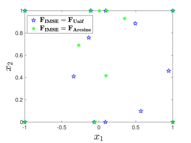
We further compare the above EI-optimal design with FIMSE(𝒙)=Funif(𝒙)subscript𝐹IMSE𝒙subscript𝐹unif𝒙F_{\operatorname{IMSE}}(\boldsymbol{x})=F_{\text{\rm unif}}(\boldsymbol{x}) to the EI-optimal design with a different FIMSE(𝒙)=Farcsine(1)(x1)Farcsine(2)(x2)subscript𝐹IMSE𝒙subscriptsuperscript𝐹1arcsinesubscript𝑥1subscriptsuperscript𝐹2arcsinesubscript𝑥2F_{\operatorname{IMSE}}(\boldsymbol{x})=F^{(1)}_{\text{\rm arcsine}}(x_{1})F^{(2)}_{\text{\rm arcsine}}(x_{2}), where Farcsine(1)(x1)superscriptsubscript𝐹arcsine1subscript𝑥1F_{\text{\rm arcsine}}^{(1)}(x_{1}) and Farcsine(2)(x2)superscriptsubscript𝐹arcsine2subscript𝑥2F_{\text{\rm arcsine}}^{(2)}(x_{2}) are arcsine distributions on [1,1]11[-1,1] and [0,1]01[0,1], respectively. Different from the uniform distribution, arcsine distribution on bounded support [a,b]𝑎𝑏[a,b] has probability density function ρ(x)=1π(xa)(xb)𝜌𝑥1𝜋𝑥𝑎𝑥𝑏\rho(x)=\frac{1}{\pi\sqrt{(x-a)(x-b)}}, x[a,b]𝑥𝑎𝑏x\in[a,b], which puts more weight towards the interval ends. Figure 2 shows the support points of EI-optimal designs when FIMSEsubscript𝐹IMSEF_{\operatorname{IMSE}} is chosen to be uniform distribution and arcsine distribution.
Refer to caption
Figure 2: Support Points of EI-Optimal Designs with FIMSE=Funifsubscript𝐹IMSEsubscript𝐹unifF_{\operatorname{IMSE}}=F_{\text{\rm unif}} and FIMSE=Farcsinesubscript𝐹IMSEsubscript𝐹arcsineF_{\operatorname{IMSE}}=F_{\text{\rm arcsine}}

Under FIMSE=Funifsubscript𝐹IMSEsubscript𝐹unifF_{\operatorname{IMSE}}=F_{\text{\rm unif}}, The efficiency of EI-optimal design achieved using arcsine distribution relative to that achieved using uniform distribution is 0.9564. On the other hand, under FIMSE=Farcsinesubscript𝐹IMSEsubscript𝐹arcsineF_{\operatorname{IMSE}}=F_{\text{\rm arcsine}}, The efficiency of EI-optimal design achieved using uniform distribution relative to that achieved using arcsine distribution is 0.9595.

Example 2. This example considers the logistic regression model with binary response. Assume that the domain of dlimit-from𝑑d-dimensional explanatory variable 𝒙=[x1,,xd]𝒙subscript𝑥1subscript𝑥𝑑\boldsymbol{x}=[x_{1},...,x_{d}] is standardized to be a unit hypercube [1,1]dsuperscript11𝑑[-1,1]^{d}. With l𝑙l basis functions 𝒈(𝒙)=[g1(𝒙),gl(𝒙)]T𝒈𝒙superscriptsubscript𝑔1𝒙subscript𝑔𝑙𝒙𝑇\boldsymbol{g}(\boldsymbol{x})=[g_{1}(\boldsymbol{x}),...g_{l}(\boldsymbol{x})]^{T} and regression coefficients 𝜷=[β1,,βl]T𝜷superscriptsubscript𝛽1subscript𝛽𝑙𝑇\boldsymbol{\beta}=[\beta_{1},...,\beta_{l}]^{T}, the logistic regression model with binary response Y{0,1}𝑌01Y\in\{0,1\} is defined as:

Prob(Y=1|𝒙)=e𝜷T𝒈(𝒙)1+e𝜷T𝒈(𝒙).𝑃𝑟𝑜𝑏𝑌conditional1𝒙superscript𝑒superscript𝜷𝑇𝒈𝒙1superscript𝑒superscript𝜷𝑇𝒈𝒙Prob(Y=1|\boldsymbol{x})=\frac{e^{\boldsymbol{\beta}^{T}\boldsymbol{g}(\boldsymbol{x})}}{1+e^{\boldsymbol{\beta}^{T}\boldsymbol{g}(\boldsymbol{x})}}.

Usually the basis functions 𝒈(𝒙)𝒈𝒙\boldsymbol{g}(\boldsymbol{x}) are low degree polynomials of explanatory variable 𝒙𝒙\boldsymbol{x}, and in this example we consider linear predictors, i.e., 𝒈(𝒙)=(1,𝒙T)T=(1,x1,,xd)T𝒈𝒙superscript1superscript𝒙𝑇𝑇superscript1subscript𝑥1subscript𝑥𝑑𝑇\boldsymbol{g}(\boldsymbol{x})=(1,\boldsymbol{x}^{T})^{T}=(1,x_{1},...,x_{d})^{T}. Given a design ξ={𝒙1,,𝒙nλ1,,λn}𝜉subscript𝒙1subscript𝒙𝑛subscript𝜆1subscript𝜆𝑛\xi=\left\{\begin{array}[]{ccc}\boldsymbol{x}_{1},&...,&\boldsymbol{x}_{n}\\ \lambda_{1},&...,&\lambda_{n}\end{array}\right\}, the EI-optimality criterion with some probability distribution FIMSEsubscript𝐹IMSEF_{\operatorname{IMSE}} is

EI(ξ,𝜷,FIMSE)=tr(𝖠𝖨(ξ)1),EI𝜉𝜷subscript𝐹IMSEtr𝖠𝖨superscript𝜉1\text{EI}(\xi,\boldsymbol{\beta},F_{\operatorname{IMSE}})=\operatorname{tr}\left({\mathsf{A}}{\mathsf{I}}(\xi)^{-1}\right),

where 𝖠=Ω(1,𝒙T)T(1,𝒙T)v(𝒙)dFIMSE(𝒙)𝖠subscriptΩsuperscript1superscript𝒙𝑇𝑇1superscript𝒙𝑇𝑣𝒙differential-dsubscript𝐹IMSE𝒙{\mathsf{A}}=\int_{\Omega}(1,\boldsymbol{x}^{T})^{T}(1,\boldsymbol{x}^{T})v(\boldsymbol{x}){\rm d}F_{\operatorname{IMSE}}(\boldsymbol{x}) with v(𝒙)=e2(β0+𝜷T𝒙)/(1+eβ0+𝜷T𝒙)4𝑣𝒙superscript𝑒2subscript𝛽0superscript𝜷𝑇𝒙superscript1superscript𝑒subscript𝛽0superscript𝜷𝑇𝒙4v(\boldsymbol{x})=e^{2(\beta_{0}+\boldsymbol{\beta}^{T}\boldsymbol{x})}/(1+e^{\beta_{0}+\boldsymbol{\beta}^{T}\boldsymbol{x}})^{4}, and 𝖨(ξ)=i=1nλiw(𝒙i)(1,𝒙iT)T(1,𝒙iT)𝖨𝜉superscriptsubscript𝑖1𝑛subscript𝜆𝑖𝑤subscript𝒙𝑖superscript1superscriptsubscript𝒙𝑖𝑇𝑇1superscriptsubscript𝒙𝑖𝑇{\mathsf{I}}(\xi)=\sum\limits_{i=1}^{n}\lambda_{i}w(\boldsymbol{x}_{i})(1,\boldsymbol{x}_{i}^{T})^{T}(1,\boldsymbol{x}_{i}^{T}) with w(𝒙i)=eβ0+𝜷T𝒙i/(1+eβ0+𝜷T𝒙i)2𝑤subscript𝒙𝑖superscript𝑒subscript𝛽0superscript𝜷𝑇subscript𝒙𝑖superscript1superscript𝑒subscript𝛽0superscript𝜷𝑇subscript𝒙𝑖2w(\boldsymbol{x}_{i})=e^{\beta_{0}+\boldsymbol{\beta}^{T}\boldsymbol{x}_{i}}/(1+e^{\beta_{0}+\boldsymbol{\beta}^{T}\boldsymbol{x}_{i}})^{2}. In this example, we consider (case i) the classical I-optimality with FIMSEsubscript𝐹IMSEF_{\operatorname{IMSE}} being a uniform distribution on Ωc=Ω=[1,1]dsubscriptΩ𝑐Ωsuperscript11𝑑\Omega_{c}=\Omega=[-1,1]^{d}, i.e., FIMSE(𝒙)=12d,𝒙Ωformulae-sequencesubscriptsuperscript𝐹IMSE𝒙1superscript2𝑑𝒙ΩF^{\prime}_{\operatorname{IMSE}}(\boldsymbol{x})=\frac{1}{2^{d}},\boldsymbol{x}\in\Omega and 𝖠=[1,1]d12d(1,𝒙T)T(1,𝒙T)v(𝒙)d𝒙𝖠subscriptsuperscript11𝑑1superscript2𝑑superscript1superscript𝒙𝑇𝑇1superscript𝒙𝑇𝑣𝒙differential-d𝒙{\mathsf{A}}=\int_{[-1,1]^{d}}\frac{1}{2^{d}}(1,\boldsymbol{x}^{T})^{T}(1,\boldsymbol{x}^{T})v(\boldsymbol{x}){\rm d}\boldsymbol{x}; and (case ii) FIMSEsubscript𝐹IMSEF_{\operatorname{IMSE}} being a uniform distribution on positive half hypercube Ωc=[0,1]dΩ=[1,1]dsubscriptΩ𝑐superscript01𝑑Ωsuperscript11𝑑\Omega_{c}=[0,1]^{d}\subset\Omega=[-1,1]^{d}, i.e., FIMSE(𝒙)={1,𝒙Ωc,0,𝒙Ωcsubscriptsuperscript𝐹IMSE𝒙cases1𝒙subscriptΩ𝑐0𝒙subscriptΩ𝑐F^{\prime}_{\operatorname{IMSE}}(\boldsymbol{x})=\left\{\begin{array}[]{ll}1,&\boldsymbol{x}\in\Omega_{c},\\ 0,&\boldsymbol{x}\notin\Omega_{c}\end{array}\right. and 𝖠=[0,1]d(1,𝒙T)T(1,𝒙T)v(𝒙)d𝒙𝖠subscriptsuperscript01𝑑superscript1superscript𝒙𝑇𝑇1superscript𝒙𝑇𝑣𝒙differential-d𝒙{\mathsf{A}}=\int_{[0,1]^{d}}(1,\boldsymbol{x}^{T})^{T}(1,\boldsymbol{x}^{T})v(\boldsymbol{x}){\rm d}\boldsymbol{x}. To investigate the performance of the proposed algorithm when the explanatory variable dimension d𝑑d gets large, we compute the EI-optimal design under the following scenarios:

  1. (a) 

    d=1𝑑1d=1, 𝜷=[0.2,1.6]T𝜷superscript0.21.6𝑇\boldsymbol{\beta}=[0.2,1.6]^{T}

  2. (b) 

    d=2𝑑2d=2, 𝜷=[2,1,2.5]T𝜷superscript212.5𝑇\boldsymbol{\beta}=[2,1,-2.5]^{T}.

  3. (c) 

    d=3𝑑3d=3, 𝜷=[0.5,1.6,2.5,2]T𝜷superscript0.51.62.52𝑇\boldsymbol{\beta}=[0.5,1.6,-2.5,2]^{T}.

We explore three properties of the proposed algorithm: (1) efficiency compared to Newton’s method; (2) choice of convergence rate δ𝛿\delta in Algorithm 1; and (3) choice of candidate pool size.

  • Efficiency compared to Newton’s method.

    The computational time comparison between the proposed algorithm and Newton’s method is summarized in Figures 3 and 4.
    Refer to caption
    Refer to caption
    (a) d=1𝑑1d=1, case i, Candidate Pool Size N=s+1𝑁𝑠1N=s+1
    Refer to caption
    Refer to caption
    (b) d=1𝑑1d=1, case ii, Candidate Pool Size N=s+1𝑁𝑠1N=s+1
    Refer to caption
    Refer to caption
    (c) d=2𝑑2d=2, case i, Candidate Pool Size N=(s+1)2𝑁superscript𝑠12N=(s+1)^{2}
    Figure 3: Computational Time (in Seconds) and Relative Efficiency Eff(ξProposed|ξNewton)Effconditionalsubscriptsuperscript𝜉Proposedsubscriptsuperscript𝜉Newton\operatorname{Eff}(\xi^{*}_{\text{Proposed}}|\xi^{*}_{\text{Newton}}) for EI-Optimal Designs with d𝑑d-Dimensional Logistic Regression Model
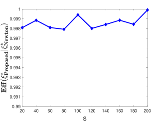
    Refer to caption
    Refer to caption
    (a) d=2𝑑2d=2, case ii, Candidate Pool Size N=(s+1)2𝑁superscript𝑠12N=(s+1)^{2}
    Refer to caption
    Refer to caption
    (b) d=3𝑑3d=3, case i, Candidate Pool Size N=(s+1)3𝑁superscript𝑠13N=(s+1)^{3}
    Figure 4: Computational Time (in Seconds) and Relative Efficiency Eff(ξProposed|ξNewton)Effconditionalsubscriptsuperscript𝜉Proposedsubscriptsuperscript𝜉Newton\operatorname{Eff}(\xi^{*}_{\text{Proposed}}|\xi^{*}_{\text{Newton}}) for EI-Optimal Designs with d𝑑d-Dimensional Logistic Regression Model (Continued)

    For d=3𝑑3d=3 of case ii, there are situations that Newton’s method does not converge in 100 iterations, i.e., the efficiency lower bound does not reach 0.99 in 100 iterations. In contrast, the proposed method is much more stable and meets the efficiency criterion in all scenarios. Thus, for d=3𝑑3d=3, we only report the computational time comparison for case i where both algorithms converge within 100 iterations. Clearly, the proposed method is quite computationally efficient. When the candidate pool size gets larger, Figure 4(c) shows that the computational times of two algorithms become close with the proposed algorithm to be slightly faster. Note that both algorithms are Wynn-Fedorov type algorithms, and the computational time is dominated by evaluating directional derivative over the large candidate pool. As the candidate pool gets large, the computational advantage of the proposed algorithm would become less pronounced. However, it is worth remarking that even with similar computational times, the proposed algorithm still has other advantages such as guaranteed convergence and simple implementation.

  • Choice of convergence rate δ𝛿\delta.

    As discussed in Section 3.2, the convergence parameter δ(0,1)𝛿01\delta\in(0,1) in Algorithm 1 is user defined and we choose δ=0.5𝛿0.5\delta=0.5 for EI-optimality. We further explore the computational time of the proposed algorithm with different choices of δ𝛿\delta ranging from 0.05 to 0.95 in d=2𝑑2d=2 of case i. The results are shown in Figure 5. It can be seen that the computational time of the proposed algorithm is quite robust to the choice δ𝛿\delta as long as δ𝛿\delta is not too small.

    Refer to caption
    Figure 5: Computational Time (in Seconds) of the Proposed Algorithm with Different Convergence Parameter δ𝛿\delta
  • Choice of candidate pool size.

    Since a discrete candidate pool 𝒞𝒞\mathcal{C} is required in Algorithm 2, discretization is needed when the experimental region is continuous. When using grid as the candidate pool, its size can increase exponentially as the dimension d𝑑d and the number of grid points in each dimension increases, and correspondingly the computational time of the proposed algorithm also increases dramatically. We explore how the size of candidate pool would influence the efficiency of the achieved design via d=2𝑑2d=2 case i. The EI-optimal designs are constructed when the candidate pool size varies from N=102𝑁superscript102N=10^{2} to N=11802𝑁superscript11802N=1180^{2}. The efficiencies of the optimal designs relative to the optimal design constructed using N=11802𝑁superscript11802N=1180^{2} are reported in Figure 5. It is not surprising that the relative efficiency does not increase monotonically as the candidate pool size increases. One explanation is that the quality of the obtained design depends on whether the candidate pool contains the support points of the optimal design with continuous experimental region, but not the size of the candidate pool. Although the candidate pool size ranges widely from N=102𝑁superscript102N=10^{2} to N=11802𝑁superscript11802N=1180^{2}, the relative efficiencies are all very close to 1 (higher than 0.999), which indicates that a very fine grid candidate pool may not be necessary to construct an EI-optimal design. Based on this observation, we would suggest using Sobol sequence as candidate design points for our proposed method when the dimension of design region d𝑑d is large.

    Refer to caption
    Figure 6: Relative Efficiency of EI-Optimal Designs with Different Candidate Pool Sizes N=(s+1)2𝑁superscript𝑠12N=(s+1)^{2}

Example 3. This example considers the Poisson regression models, which is a popular statistical tool to model count data in many applications (e.g., Gart 1964; El-Shaarawi et al. 1987). Like in Example 2, we assume that the domain of dlimit-from𝑑d-dimensional explanatory variable 𝒙=[x1,,xd]𝒙subscript𝑥1subscript𝑥𝑑\boldsymbol{x}=[x_{1},...,x_{d}] is standardized to be a unit hypercube Ω=[1,1]dΩsuperscript11𝑑\Omega=[-1,1]^{d}. With l𝑙l basis functions 𝒈(𝒙)=[g1(𝒙),gl(𝒙)]T𝒈𝒙superscriptsubscript𝑔1𝒙subscript𝑔𝑙𝒙𝑇\boldsymbol{g}(\boldsymbol{x})=[g_{1}(\boldsymbol{x}),...g_{l}(\boldsymbol{x})]^{T} and regression coefficients 𝜷=[β1,,βl]T𝜷superscriptsubscript𝛽1subscript𝛽𝑙𝑇\boldsymbol{\beta}=[\beta_{1},...,\beta_{l}]^{T}, the Poisson regression model with count response Y{0,1,,}Y\in\{0,1,...,\} has the mean function:

μ(𝒙)=𝔼[Y(𝒙)]=e𝜷T𝒈(𝒙).𝜇𝒙𝔼delimited-[]𝑌𝒙superscript𝑒superscript𝜷𝑇𝒈𝒙\mu(\boldsymbol{x})=\mathbb{E}[Y(\boldsymbol{x})]=e^{\boldsymbol{\beta}^{T}\boldsymbol{g}(\boldsymbol{x})}.

Similar as Example 2, we consider linear predictors, i.e., 𝒈(𝒙)=(1,𝒙T)T=(1,x1,,xd)T𝒈𝒙superscript1superscript𝒙𝑇𝑇superscript1subscript𝑥1subscript𝑥𝑑𝑇\boldsymbol{g}(\boldsymbol{x})=(1,\boldsymbol{x}^{T})^{T}=(1,x_{1},...,x_{d})^{T}. Given a design ξ={𝒙1,,𝒙nλ1,,λn}𝜉subscript𝒙1subscript𝒙𝑛subscript𝜆1subscript𝜆𝑛\xi=\left\{\begin{array}[]{ccc}\boldsymbol{x}_{1},&...,&\boldsymbol{x}_{n}\\ \lambda_{1},&...,&\lambda_{n}\end{array}\right\}, the classical I-optimality criterion with FIMSE=Funifsubscript𝐹IMSEsubscript𝐹unifF_{\operatorname{IMSE}}=F_{\text{\rm unif}} on [1,1]dsuperscript11𝑑[-1,1]^{d} is

EI(ξ,𝜷,Funif)=tr(𝖠𝖨(ξ)1),EI𝜉𝜷subscript𝐹uniftr𝖠𝖨superscript𝜉1\text{EI}(\xi,\boldsymbol{\beta},F_{\text{\rm unif}})=\operatorname{tr}\left({\mathsf{A}}{\mathsf{I}}(\xi)^{-1}\right),

with 𝖠=12d(1,𝒙T)T(1,𝒙T)e2(β0+𝜷T𝒙)d𝒙𝖠1superscript2𝑑superscript1superscript𝒙𝑇𝑇1superscript𝒙𝑇superscript𝑒2subscript𝛽0superscript𝜷𝑇𝒙differential-d𝒙{\mathsf{A}}=\int\frac{1}{2^{d}}(1,\boldsymbol{x}^{T})^{T}(1,\boldsymbol{x}^{T})e^{2\left(\beta_{0}+\boldsymbol{\beta}^{T}\boldsymbol{x}\right)}{\rm d}\boldsymbol{x} and 𝖨(ξ)=i=1nλieβ0+𝜷T𝒙i(1,𝒙iT)T(1,𝒙iT)𝖨𝜉superscriptsubscript𝑖1𝑛subscript𝜆𝑖superscript𝑒subscript𝛽0superscript𝜷𝑇subscript𝒙𝑖superscript1superscriptsubscript𝒙𝑖𝑇𝑇1superscriptsubscript𝒙𝑖𝑇{\mathsf{I}}(\xi)=\sum\limits_{i=1}^{n}\lambda_{i}e^{\beta_{0}+\boldsymbol{\beta}^{T}\boldsymbol{x}_{i}}(1,\boldsymbol{x}_{i}^{T})^{T}(1,\boldsymbol{x}_{i}^{T}). We consider the same scenarios as in Example 2 for Poisson regression model and compute the corresponding classical I-optimal designs:

  1. (a) 

    d=1𝑑1d=1, 𝜷=[0.2,1.6]T𝜷superscript0.21.6𝑇\boldsymbol{\beta}=[0.2,1.6]^{T}

  2. (b) 

    d=2𝑑2d=2, 𝜷=[2,1,2.5]T𝜷superscript212.5𝑇\boldsymbol{\beta}=[2,1,-2.5]^{T}.

  3. (c) 

    d=3𝑑3d=3, 𝜷=[0.5,1.6,2.5,2]T𝜷superscript0.51.62.52𝑇\boldsymbol{\beta}=[0.5,1.6,-2.5,2]^{T}.

Here we also use the grids to form the set of candidate design points. The computation comparison is shown in Figure 7. Similar to the results in Example 2, when the candidate pool size is moderate, the proposed algorithm outperforms the Newton’s method by a large margin regarding the computational efficiency, and also preserves a high design efficiency.
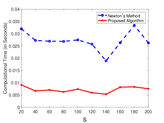
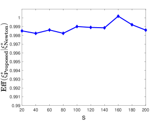
Refer to caption
Refer to caption
(a) d=1𝑑1d=1, Candidate Pool Size N=s+1𝑁𝑠1N=s+1
Refer to caption
Refer to caption
(b) d=2𝑑2d=2, Candidate Pool Size N=(s+1)2𝑁superscript𝑠12N=(s+1)^{2}
Refer to caption
Refer to caption
(c) d=3𝑑3d=3, Candidate Pool Size N=(s+1)3𝑁superscript𝑠13N=(s+1)^{3}
Figure 7: Computational Time (in Seconds) and Relative Efficiency Eff(ξProposed|ξNewton)Effconditionalsubscriptsuperscript𝜉Proposedsubscriptsuperscript𝜉Newton\operatorname{Eff}(\xi^{*}_{\text{Proposed}}|\xi^{*}_{\text{Newton}}) for EI-Optimal Designs with d𝑑d-Dimensional Poisson Regression Model

Example 4. In this example, we would like to provide some comparison between EI-optimal design and other parameter estimation oriented D- and A-optimal designs through a real-world potato packing example in Woods et al. (2006). The experiment contains d=3𝑑3d=3 quantitative variables - vitamin concentration in the prepackaging dip and levels of two gases in the packing atmosphere. The response is binary representing the presence or absence of liquid in the pack after 7 days. All explanatory variables are standardized, and the experimental region Ω=[1,1]3Ωsuperscript113\Omega=[-1,1]^{3}. We consider one of the candidate models used in the real study: a logit model with quadratic basis. The estimates of regression coefficients from preliminary study are given in Table 1. FIMSE=Funifsubscript𝐹IMSEsubscript𝐹unifF_{\operatorname{IMSE}}=F_{\text{\rm unif}} on ΩΩ\Omega is used to define EI-optimality.

Table 1: Logit Model of Potato Packing Example
Term Intercept x2subscript𝑥2x_{2} x3subscript𝑥3x_{3} x2x3subscript𝑥2subscript𝑥3x_{2}x_{3} x12superscriptsubscript𝑥12x_{1}^{2} x22superscriptsubscript𝑥22x_{2}^{2} x32superscriptsubscript𝑥32x_{3}^{2}
Coefficient -2.93 -0.52 -0.79 -0.66 0.94 0.79 1.82

Figure 8 shows the support points of D-, A- and EI-Optimal Designs. The relative EI-efficiency of D- and A- optimal designs relative to EI-optimal design are 80.64%percent80.6480.64\% and 85.44%percent85.4485.44\%, respectively. To some extent, this demonstrates the importance and necessity of accurate estimate of regression coefficients to make precise prediction, but D- or A-optimality may not be the most appropriate criterion to use when the prediction is of interest. The relative A- and D-efficiency of the EI-optimal design relative to the corresponding A- and D-optimal designs are 81.12%percent81.1281.12\% and 88.76%percent88.7688.76\%, respectively. Thus, it is important to choose the appropriate optimality criterion based on the purpose of the experiment.
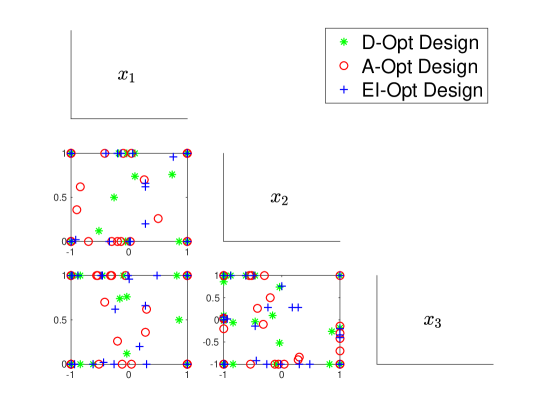
Refer to caption
Figure 8: Support Points of D-, A- and EI-Optimal Designs

6 Discussion

In this work, we study a general and flexible prediction-oriented criterion EI-optimality for GLMs and advance an efficient sequential algorithm with sound convergence properties for constructing EI-optimal designs. Through a deep investigation on the theoretical properties of the EI-optimality, we have obtained an insightful understanding for the proposed algorithm on how to sequentially choose the support point and update the weights of support points of the design. The computational advantages of the proposed algorithm over the Newton’s method is demonstrated through numerical examples with moderate size candidate pools for various types of GLMs. Moreover, all the computations in the proposed algorithm are explicit and simple to implement. The proposed method exemplifies a good case on the integration of theory and computation to advance the development of new statistical methodology.

It is worth remarking that the proposed sequential algorithm (Algorithm 2) is not restricted to the EI-optimality for constructing optimal designs. The proposed sequential algorithm can be extended to other optimality criteria when the directional derivative ϕ(ξ,ξ)italic-ϕsuperscript𝜉𝜉\phi(\xi^{\prime},\xi) of optimality criterion in (8) exists. Although the convergence property of the proposed algorithm (Theorem 5) in Section 4.2 is stated in the context of EI-optimality, a proof on the convergence of the proposed algorithm for general ΦpsubscriptΦ𝑝\Phi_{p}-optimality is provided in the appendix. As the EI-optimlity has the same mathematical structure as Φ1subscriptΦ1\Phi_{1}-optimality, the convergence of the algorithm still holds. Note that this work focuses on the local EI-optimal designs for the generalized linear models, which depends on given regression coefficients. The parameter dependence problem in the design of GLMs is an important yet challenging issue (Khuri et al. 2006; Woods et al. 2006). For instance, the EI-efficiency of the compromise design proposed by Woods et al. (2006) relative to the local EI-optimal design under three model specifications (see Woods et al. 2006) are 49%percent4949\%, 80%percent8080\% and 92%percent9292\%. Bayesian or pseudo-Bayesian approaches are generally recognized as an appealing solution to address the parameter dependence issue. For our proposed method of EI-optimal design, we will further investigate the robust EI-optimal design for the GLMs. One possibility is to establish a tight upper bound for the integrated mean squared error to relax the dependency on the regression coefficients. Then we can modify the proposed algorithm in search of optimal designs based on the robust optimality criterion constructed according to the upper bound. Hickernell and Liu (2002) developed some theoretical results in a similar direction for linear regression models under model uncertainty, and Li and Hickernell (2014) extended the results to linear regression models with gradient information.

We would like to remark that the proposed method may not have great computational efficiency when the candidate pool gets very large. One direction for tackling this issue is to better take advantage of the information on probability measure in the design region for constructing the design. For example, one can modify the selection of candidate pool based on the probability measure in the design region. Another interesting point is that the support points in the optimal design can be outside of the prediction region of interest, which could be a potential limitation of the proposed method.

For future research, it will be interesting to construct EI-optimal designs for the models with both quantitative and qualitative responses (Deng and Jin 2015). Since the GLMs include both the linear regression for continuous response and the logistic regression for binary response, it would be interesting to study the EI-optimal designs under the consideration of jointly modeling both quantitative and qualitative responses. Finally, the proposed sequential algorithm is not restricted to find desirable designs for physical experiments. It can be applied for finding space-filling design in computer experiments (Deng et al. 2015).

References

  • Atkinson 2014 Atkinson, A. C. (2014), “Optimal design,” Wiley StatsRef: Statistics Reference Online, 1–17.
  • Atkinson et al. 2006 Atkinson, A. C., Donev, A. N., and Tobias, R. D. (2006), Optimum Experimental Designs, with SAS, Oxford University Press.
  • Atkinson and Woods 2015 Atkinson, A. C. and Woods, D. C. (2015), “Designs for generalized linear models,” Handbook of Design and Analysis of Experiments, 471–514.
  • Atwood 1969 Atwood, C. L. (1969), “Optimal and efficient designs of experiments,” The Annals of Mathematical Statistics, 1570–1602.
  • Bernstein 2009 Bernstein, D. S. (2009), Matrix Mathematics (2nd Edition), Princeton University Press.
  • Bilgic et al. 2010 Bilgic, M., Mihalkova, L., and Getoor, L. (2010), “Active learning for networked data,” in Proceedings of the 27th international conference on machine learning (ICML-10), pp. 79–86.
  • Box and Draper 1963 Box, G. E. and Draper, N. R. (1963), “The choice of a second order rotatable design,” Biometrika, 335–352.
  • Deng et al. 2015 Deng, X., Hung, Y., and Lin, C. D. (2015), “Design for computer experiments with qualitative and quantitative factors,” Statistica Sinica, 1567–1581.
  • Deng and Jin 2015 Deng, X. and Jin, R. (2015), “QQ Models: Joint Modeling for Quantitative and Qualitative Quality Responses in Manufacturing Systems,” Technometrics, 57, 320–331.
  • El-Shaarawi et al. 1987 El-Shaarawi, A., Maul, A., and Block, J.-C. (1987), “Application of Poisson regression to the analysis of bacteriological data,” Water Quality Research Journal, 22, 298–307.
  • Fedorov 1972 Fedorov, V. V. (1972), Theory of Optimal Experiments, New York: Academic Press.
  • Fedorov and Hackl 1997 Fedorov, V. V. and Hackl, P. (1997), Model-Oriented Design of Experiments, vol. 125, Springer Science & Business Media.
  • Fellman 1974 Fellman, J. (1974), On the Allocation of Linear Observations, Societas Scientiarum Fennica.
  • Fiacco and Kortanek 1983 Fiacco, A. V. and Kortanek, K. O. (eds.) (1983), A Moment Inequality and Monotonicity of an Algorithm.
  • Gart 1964 Gart, J. J. (1964), “The analysis of Poisson regression with an application in virology,” Biometrika, 51, 517–521.
  • Haines 1987 Haines, L. M. (1987), “The Application of the Annealing Algorithm to the Construction of Exact Optimal Designs for Linear-Regression Models,” Technometrics, 29, 439–447.
  • Harman et al. 2019 Harman, R., Filová, L., and Richtárik, P. (2019), “A randomized exchange algorithm for computing optimal approximate designs of experiments,” Journal of the American Statistical Association, 1–30.
  • Hickernell and Liu 2002 Hickernell, F. J. and Liu, M. (2002), “Uniform designs limit aliasing,” Biometrika, 89, 893–904.
  • Khuri et al. 2006 Khuri, A. I., Mukherjee, B., Sinha, B. K., and Ghosh, M. (2006), “Design Issues for Generalized Linear Models,” Technometrics, 48, 520–529.
  • Kiefer 1974 Kiefer, J. (1974), “General equivalence theory for optimum designs (approximate theory),” The annals of Statistics, 849–879.
  • Kiefer 1985 — (1985), “Optimal Design: Variation in Structure and Performance Under Change of Criterion,” Biometrika, 62, 277–288.
  • Li and Hickernell 2014 Li, Y. and Hickernell, F. J. (2014), “Design of experiments for linear regression models when gradient information is available,” Journal of Statistical Planning and Inference, 144, 141–151.
  • Martín and Gutiérrez 2015 Martín, R. M. and Gutiérrez, I. G. C. (2015), “Combined algorithm to compute D-optimal designs,” Journal of Computational and Applied Mathematics, 278, 248–257.
  • Meyer and Nachtsheim 1988 Meyer, R. K. and Nachtsheim, C. J. (1988), “Simulated Annealing in the Construction of Exact Optimal Design of Experiments,” American Journal of Mathematical and Management Science, 8.
  • Meyer and Nachtsheim 1995 — (1995), “The Coordinate-Exchange Algorithm for Constructing Exact Optimal Experimental Designs,” Technometrics, 37, 60–69.
  • Nelder and Wedderburn 1972 Nelder, J. and Wedderburn, R. (1972), “Generalized Linear Models,” Journal of Royal Statistical Society-Series B, 135, 370–384.
  • Pukelsheim 1993 Pukelsheim, F. (1993), Optimal Design of Experiments, John Wiley &\& Sons, Inc.
  • Pukelsheim 2006 — (2006), Optimal design of experiments, SIAM.
  • Pursell and Trimble 1991 Pursell, L. and Trimble, S. T. (1991), “Gram-Schmidt Orthogonalization by Gauss Elimination,” The American Mathematical Monthly, 98, 544–549.
  • Schein and Ungar 2007 Schein, A. I. and Ungar, L. H. (2007), “Active Learning for Logistic Regression: An Evaluation,” Machine Learning, 68, 235–265.
  • Settles 2009 Settles, B. (2009), “Active learning literature survey,” Tech. rep., University of Wisconsin-Madison Department of Computer Sciences.
  • Silvey et al. 1978 Silvey, S. D., Titterington, D. M., and Torsney, B. (1978), “An algorithm for optimal designs on a finite design space,” Communications in Statistics - Theory and Methods, 14, 1379–1389.
  • Sobol 1967 Sobol, I. M. (1967), “On the Distribution of Points in a Cube and the Approximate Evaluation of Integrals,” USSR Computational Mathematics and Mathematical Physics, 7, 86–112.
  • Stufken and Yang 2011 Stufken, J. and Yang, M. (2011), “Optimal designs for generalized linear models,” Design and Analysis of Experiments, Volume 3: Special Designs and Applications, 810, 137.
  • Sun et al. 2018 Sun, H., Rao, P. K., Kong, Z. J., Deng, X., and Jin, R. (2018), “Functional quantitative and qualitative models for quality modeling in a fused deposition modeling process,” IEEE Transactions on Automation Science and Engineering, 15, 393–403.
  • Titterington 1978 Titterington, D. M. (1978), “Estimation of Correlation Coefficients by Ellipsoidal Trimming,” Applied Statistics, 27, 227–234.
  • Whittle 1973 Whittle, P. (1973), “Some General Points in the Theory of Optimal Experimental Design,” Journal of Royal Statistical Society-Series B, 35, 123–130.
  • Woods et al. 2006 Woods, D. C., Lewis, S. M., Eccleston, J. A., and Russell, K. (2006), “Designs for generalized linear models with several variables and model uncertainty,” Technometrics, 48, 284–292.
  • Wynn 1970 Wynn, H. (1970), “The Sequential Generation of D-optimum Experimental Designs,” Annals of Mathematical Statistics, A 7, 1399–1412.
  • Wynn 1972 Wynn, H. P. (1972), “Results in the Theory and Construction of D-Optimum Experimental Designs,” Journal of Royal Statistical Society-Series B, 34, 133–147.
  • Yang et al. 2016 Yang, J., Mandal, A., and Majumdar, D. (2016), “Optimal Designs for 2ksuperscript2𝑘2^{k} Factorial Experiments with Binary Response,” Statistica Sinica, 385–411.
  • Yang et al. 2013 Yang, M., Biedermann, S., and Tang, E. (2013), “On Optimal Designs for Nonlinear Models: A general and Efficient Algorithm,” Journal of the American Statistical Association, 108, 1411–1420.
  • Yang and Stufken 2012 Yang, M. and Stufken, J. (2012), “Identifying Locally Optimal Designs for Nonlinear Models: A Simple Extension with Profound Consequences,” The Annals of Statistics, 40, 1665–1681.
  • Yu 2010 Yu, Y. (2010), “Monotonic Convergence of a General Algorithm for Computing Optimal Designs,” The Annals of Statistics, 38, 1593–1606.

Appendix

Proof of Lemma 1

Proof.
EI(ξ,𝜷,FIMSE)EI𝜉𝜷subscript𝐹IMSE\displaystyle\text{EI}(\xi,\boldsymbol{\beta},F_{\operatorname{IMSE}}) =\displaystyle= 𝔼[Ω𝒄(𝒙)T(𝜷^𝜷)(𝜷^𝜷)T𝒄(𝒙)dFIMSE(𝒙)]𝔼delimited-[]subscriptΩ𝒄superscript𝒙𝑇^𝜷𝜷superscript^𝜷𝜷𝑇𝒄𝒙differential-dsubscript𝐹IMSE𝒙\displaystyle\mathbb{E}\left[\int_{\Omega}\boldsymbol{c}(\boldsymbol{x})^{T}\left(\hat{\boldsymbol{\beta}}-\boldsymbol{\beta}\right)\left(\hat{\boldsymbol{\beta}}-\boldsymbol{\beta}\right)^{T}\boldsymbol{c}(\boldsymbol{x}){\rm d}F_{\operatorname{IMSE}}(\boldsymbol{x})\right]
=\displaystyle= Ω𝒄(𝒙)T𝔼[(𝜷^𝜷)(𝜷^𝜷)T]𝒄(𝒙)dFIMSE(𝒙)subscriptΩ𝒄superscript𝒙𝑇𝔼delimited-[]^𝜷𝜷superscript^𝜷𝜷𝑇𝒄𝒙differential-dsubscript𝐹IMSE𝒙\displaystyle\int_{\Omega}\boldsymbol{c}(\boldsymbol{x})^{T}\mathbb{E}\left[\left(\hat{\boldsymbol{\beta}}-\boldsymbol{\beta}\right)\left(\hat{\boldsymbol{\beta}}-\boldsymbol{\beta}\right)^{T}\right]\boldsymbol{c}(\boldsymbol{x}){\rm d}F_{\operatorname{IMSE}}(\boldsymbol{x})
\displaystyle\approx Ωtr(𝒄(𝒙)𝒄(𝒙)T𝖨(ξ,𝜷)1)dFIMSE(𝒙)subscriptΩtr𝒄𝒙𝒄superscript𝒙𝑇𝖨superscript𝜉𝜷1differential-dsubscript𝐹IMSE𝒙\displaystyle\int_{\Omega}\operatorname{tr}\left(\boldsymbol{c}(\boldsymbol{x})\boldsymbol{c}(\boldsymbol{x})^{T}{\mathsf{I}}\left(\xi,\boldsymbol{\beta}\right)^{-1}\right){\rm d}F_{\operatorname{IMSE}}(\boldsymbol{x})
=\displaystyle= tr[(Ω𝒄(𝒙)𝒄(𝒙)TdFIMSE(𝒙))𝖨(ξ,𝜷)1]trsubscriptΩ𝒄𝒙𝒄superscript𝒙𝑇differential-dsubscript𝐹IMSE𝒙𝖨superscript𝜉𝜷1\displaystyle\operatorname{tr}\left[\left(\int_{\Omega}\boldsymbol{c}(\boldsymbol{x})\boldsymbol{c}(\boldsymbol{x})^{T}{\rm d}F_{\operatorname{IMSE}}(\boldsymbol{x})\right){\mathsf{I}}(\xi,\boldsymbol{\beta})^{-1}\right]
=\displaystyle= tr(𝖠𝖨(ξ,𝜷)1).tr𝖠𝖨superscript𝜉𝜷1\displaystyle\operatorname{tr}\left({\mathsf{A}}{\mathsf{I}}(\xi,\boldsymbol{\beta})^{-1}\right).

The approximation is provided by the fact that the estimated regression coefficient 𝜷^^𝜷\hat{\boldsymbol{\beta}} follows N(𝜷,𝖨(ξ,𝜷)1)𝑁𝜷𝖨superscript𝜉𝜷1N(\boldsymbol{\beta},{\mathsf{I}}(\xi,\boldsymbol{\beta})^{-1}) asymptotically. ∎

Proof of Lemma 2

Proof.

For matrix 𝒇(𝜷)𝜷T𝒇𝜷superscript𝜷𝑇\frac{\partial\boldsymbol{f}(\boldsymbol{\beta})}{\partial\boldsymbol{\beta}^{T}} with size q×l𝑞𝑙q\times l and matrix 𝖨(ξ𝝀)1(𝒇(𝜷)𝜷T)T𝖨superscriptsuperscript𝜉𝝀1superscript𝒇𝜷superscript𝜷𝑇𝑇{\mathsf{I}}(\xi^{\boldsymbol{\lambda}})^{-1}\left(\frac{\partial\boldsymbol{f}(\boldsymbol{\beta})}{\partial\boldsymbol{\beta}^{T}}\right)^{T} with size l×q𝑙𝑞l\times q, and ql𝑞𝑙q\leq l, the eigenvalues of 𝒇(𝜷)𝜷T𝖨(ξ𝝀)1(𝒇(𝜷)𝜷T)T𝒇𝜷superscript𝜷𝑇𝖨superscriptsuperscript𝜉𝝀1superscript𝒇𝜷superscript𝜷𝑇𝑇\frac{\partial\boldsymbol{f}(\boldsymbol{\beta})}{\partial\boldsymbol{\beta}^{T}}{\mathsf{I}}(\xi^{\boldsymbol{\lambda}})^{-1}\left(\frac{\partial\boldsymbol{f}(\boldsymbol{\beta})}{\partial\boldsymbol{\beta}^{T}}\right)^{T} are the eigenvalues of 𝖨(ξ𝝀)1(𝒇(𝜷)𝜷T)T𝒇(𝜷)𝜷T𝖨superscriptsuperscript𝜉𝝀1superscript𝒇𝜷superscript𝜷𝑇𝑇𝒇𝜷superscript𝜷𝑇{\mathsf{I}}(\xi^{\boldsymbol{\lambda}})^{-1}\left(\frac{\partial\boldsymbol{f}(\boldsymbol{\beta})}{\partial\boldsymbol{\beta}^{T}}\right)^{T}\frac{\partial\boldsymbol{f}(\boldsymbol{\beta})}{\partial\boldsymbol{\beta}^{T}}, with extra eigenvalues being 0 if there is any. Thus, the eigenvalues of[𝖨(ξ𝝀)1(𝒇(𝜷)𝜷T)T𝒇(𝜷)𝜷T]psuperscriptdelimited-[]𝖨superscriptsuperscript𝜉𝝀1superscript𝒇𝜷superscript𝜷𝑇𝑇𝒇𝜷superscript𝜷𝑇𝑝\left[{\mathsf{I}}(\xi^{\boldsymbol{\lambda}})^{-1}\left(\frac{\partial\boldsymbol{f}(\boldsymbol{\beta})}{\partial\boldsymbol{\beta}^{T}}\right)^{T}\frac{\partial\boldsymbol{f}(\boldsymbol{\beta})}{\partial\boldsymbol{\beta}^{T}}\right]^{p} are the eigenvalues of [𝒇(𝜷)𝜷T𝖨(ξ𝝀)1(𝒇(𝜷)𝜷T)T]psuperscriptdelimited-[]𝒇𝜷superscript𝜷𝑇𝖨superscriptsuperscript𝜉𝝀1superscript𝒇𝜷superscript𝜷𝑇𝑇𝑝\left[\frac{\partial\boldsymbol{f}(\boldsymbol{\beta})}{\partial\boldsymbol{\beta}^{T}}{\mathsf{I}}(\xi^{\boldsymbol{\lambda}})^{-1}\left(\frac{\partial\boldsymbol{f}(\boldsymbol{\beta})}{\partial\boldsymbol{\beta}^{T}}\right)^{T}\right]^{p} with extra eigenvalues being 0. Thus, we could rewrite

tr[𝒇(𝜷)𝜷T𝖨(ξ𝝀)1(𝒇(𝜷)𝜷T)T]p=tr[𝖨(ξ𝝀)1(𝒇(𝜷)𝜷T)T(𝒇(𝜷)𝜷T)]p=tr[𝖨1(ξ𝝀)𝖡]p,\displaystyle\operatorname{tr}\left[\frac{\partial\boldsymbol{f}(\boldsymbol{\beta})}{\partial\boldsymbol{\beta}^{T}}{\mathsf{I}}(\xi^{\boldsymbol{\lambda}})^{-1}\left(\frac{\partial\boldsymbol{f}(\boldsymbol{\beta})}{\partial\boldsymbol{\beta}^{T}}\right)^{T}\right]^{p}=\operatorname{tr}\left[{\mathsf{I}}(\xi^{\boldsymbol{\lambda}})^{-1}\left(\frac{\partial\boldsymbol{f}(\boldsymbol{\beta})}{\partial\boldsymbol{\beta}^{T}}\right)^{T}\left(\frac{\partial\boldsymbol{f}(\boldsymbol{\beta})}{\partial\boldsymbol{\beta}^{T}}\right)\right]^{p}=\operatorname{tr}\left[{\mathsf{I}}^{-1}(\xi^{\boldsymbol{\lambda}}){\mathsf{B}}\right]^{p}, (10)

where 𝖡=(𝒇(𝜷)𝜷T)T(𝒇(𝜷)𝜷T)𝖡superscript𝒇𝜷superscript𝜷𝑇𝑇𝒇𝜷superscript𝜷𝑇{\mathsf{B}}=\left(\frac{\partial\boldsymbol{f}(\boldsymbol{\beta})}{\partial\boldsymbol{\beta}^{T}}\right)^{T}\left(\frac{\partial\boldsymbol{f}(\boldsymbol{\beta})}{\partial\boldsymbol{\beta}^{T}}\right) which is positive semidefinite with size l×l𝑙𝑙l\times l and rank ql𝑞𝑙q\leq l. Then, by Smith decomposition, there exists a nonsingular matrix 𝖲𝖲{\mathsf{S}} of size l×l𝑙𝑙l\times l such that

𝖡=𝖲T(𝑰q𝟎q×(lq)𝟎(lq)×q𝟎(lq)×(lq))𝖲=𝖲T(𝑰q𝟎(lq)×q)(𝑰q     0q×(lq))𝖲,𝖡superscript𝖲𝑇subscript𝑰𝑞subscript0𝑞𝑙𝑞subscript0𝑙𝑞𝑞subscript0𝑙𝑞𝑙𝑞𝖲superscript𝖲𝑇subscript𝑰𝑞subscript0𝑙𝑞𝑞subscript𝑰𝑞subscript     0𝑞𝑙𝑞𝖲{\mathsf{B}}={\mathsf{S}}^{T}\left(\begin{array}[]{cc}\boldsymbol{I}_{q}&\boldsymbol{0}_{q\times(l-q)}\\ \boldsymbol{0}_{(l-q)\times q}&\boldsymbol{0}_{(l-q)\times(l-q)}\end{array}\right){\mathsf{S}}={\mathsf{S}}^{T}\left(\begin{array}[]{c}\boldsymbol{I}_{q}\\ \boldsymbol{0}_{(l-q)\times q}\end{array}\right)\left(\boldsymbol{I}_{q}\,\,\,\,\,\boldsymbol{0}_{q\times(l-q)}\right){\mathsf{S}},

where 𝑰qsubscript𝑰𝑞\boldsymbol{I}_{q} is the identity matrix of size q×q𝑞𝑞q\times q. Thus, Equation (10) could be written as

tr[𝒇(𝜷)𝜷T𝖨(ξ𝝀)1(𝒇(𝜷)𝜷T)T]p\displaystyle\operatorname{tr}\left[\frac{\partial\boldsymbol{f}(\boldsymbol{\beta})}{\partial\boldsymbol{\beta}^{T}}{\mathsf{I}}(\xi^{\boldsymbol{\lambda}})^{-1}\left(\frac{\partial\boldsymbol{f}(\boldsymbol{\beta})}{\partial\boldsymbol{\beta}^{T}}\right)^{T}\right]^{p} (13)
=\displaystyle= tr[𝖨(ξ𝝀)1𝖲T(𝑰q𝟎(lq)×q)(𝑰q     0q×(lq))𝖲]p\displaystyle\operatorname{tr}\left[{\mathsf{I}}(\xi^{\boldsymbol{\lambda}})^{-1}{\mathsf{S}}^{T}\left(\begin{array}[]{c}\boldsymbol{I}_{q}\\ \boldsymbol{0}_{(l-q)\times q}\end{array}\right)\left(\boldsymbol{I}_{q}\,\,\,\,\,\boldsymbol{0}_{q\times(l-q)}\right){\mathsf{S}}\right]^{p}
=\displaystyle= tr{[(𝑰q     0q×(lq))((𝖲T)1𝖨(ξ𝝀)𝖲1)1(𝑰q𝟎(lq)×q)]1}p.\displaystyle\operatorname{tr}\left\{\left[\left(\boldsymbol{I}_{q}\,\,\,\,\,\boldsymbol{0}_{q\times(l-q)}\right)\left(({\mathsf{S}}^{T})^{-1}{\mathsf{I}}(\xi^{\boldsymbol{\lambda}}){\mathsf{S}}^{-1}\right)^{-1}\left(\begin{array}[]{c}\boldsymbol{I}_{q}\\ \boldsymbol{0}_{(l-q)\times q}\end{array}\right)\right]^{-1}\right\}^{-p}. (16)

Consider two weights 𝝀1subscript𝝀1\boldsymbol{\lambda}_{1} and 𝝀2subscript𝝀2\boldsymbol{\lambda}_{2}, and define 𝝀3=(1a)𝝀1+a𝝀2subscript𝝀31𝑎subscript𝝀1𝑎subscript𝝀2\boldsymbol{\lambda}_{3}=(1-a)\boldsymbol{\lambda}_{1}+a\boldsymbol{\lambda}_{2}. With 0a10𝑎10\leq a\leq 1, 𝝀3subscript𝝀3\boldsymbol{\lambda}_{3} is still a feasible weight vector, and

(𝖲T)1𝖨(ξ𝝀3)𝖲1=(1a)(𝖲T)1𝖨(ξ𝝀1)𝖲1+a(𝖲T)1𝖨(ξ𝝀2)𝖲1.superscriptsuperscript𝖲𝑇1𝖨superscript𝜉subscript𝝀3superscript𝖲11𝑎superscriptsuperscript𝖲𝑇1𝖨superscript𝜉subscript𝝀1superscript𝖲1𝑎superscriptsuperscript𝖲𝑇1𝖨superscript𝜉subscript𝝀2superscript𝖲1\displaystyle({\mathsf{S}}^{T})^{-1}{\mathsf{I}}(\xi^{\boldsymbol{\lambda}_{3}}){\mathsf{S}}^{-1}=(1-a)({\mathsf{S}}^{T})^{-1}{\mathsf{I}}(\xi^{\boldsymbol{\lambda}_{1}}){\mathsf{S}}^{-1}+a({\mathsf{S}}^{T})^{-1}{\mathsf{I}}(\xi^{\boldsymbol{\lambda}_{2}}){\mathsf{S}}^{-1}. (17)

By the theorem in section 3.13 of Pukelsheim (1993),

[(𝑰q     0q×(lq))((𝖲T)1𝖨(ξ𝝀)𝖲1)1(𝑰q     0(lq)×q)T]1superscriptdelimited-[]subscript𝑰𝑞subscript     0𝑞𝑙𝑞superscriptsuperscriptsuperscript𝖲𝑇1𝖨superscript𝜉𝝀superscript𝖲11superscriptsubscript𝑰𝑞subscript     0𝑙𝑞𝑞𝑇1\displaystyle\left[\left(\boldsymbol{I}_{q}\,\,\,\,\,\boldsymbol{0}_{q\times(l-q)}\right)\left(({\mathsf{S}}^{T})^{-1}{\mathsf{I}}(\xi^{\boldsymbol{\lambda}}){\mathsf{S}}^{-1}\right)^{-1}\left(\boldsymbol{I}_{q}\,\,\,\,\,\boldsymbol{0}_{(l-q)\times q}\right)^{T}\right]^{-1} (18)

is matrix concave in (𝖲T)1𝖨(ξ𝝀)𝖲1superscriptsuperscript𝖲𝑇1𝖨superscript𝜉𝝀superscript𝖲1({\mathsf{S}}^{T})^{-1}{\mathsf{I}}(\xi^{\boldsymbol{\lambda}}){\mathsf{S}}^{-1}. Thus, by linearity of matrix (𝖲T)1𝖨(ξ𝝀)𝖲1superscriptsuperscript𝖲𝑇1𝖨superscript𝜉𝝀superscript𝖲1({\mathsf{S}}^{T})^{-1}{\mathsf{I}}(\xi^{\boldsymbol{\lambda}}){\mathsf{S}}^{-1} in weight in (17), [(𝑰q     0q×(lq))((𝖲T)1𝖨(ξ𝝀)𝖲1)1(𝑰q     0(lq)×q)T]1superscriptdelimited-[]subscript𝑰𝑞subscript     0𝑞𝑙𝑞superscriptsuperscriptsuperscript𝖲𝑇1𝖨superscript𝜉𝝀superscript𝖲11superscriptsubscript𝑰𝑞subscript     0𝑙𝑞𝑞𝑇1\left[\left(\boldsymbol{I}_{q}\,\,\,\,\,\boldsymbol{0}_{q\times(l-q)}\right)\left(({\mathsf{S}}^{T})^{-1}{\mathsf{I}}(\xi^{\boldsymbol{\lambda}}){\mathsf{S}}^{-1}\right)^{-1}\left(\boldsymbol{I}_{q}\,\,\,\,\,\boldsymbol{0}_{(l-q)\times q}\right)^{T}\right]^{-1} is also concave in weight vector 𝝀𝝀\boldsymbol{\lambda}.

Since tr(𝖢p)1/p\operatorname{tr}({\mathsf{C}}^{-p})^{1/p} is nonincreasing and convex for any positive semidefinite matrix 𝖢𝖢{\mathsf{C}} (Fedorov and Hackl 1997, see page 22), together with concavity of (18), the composite function

[tr{[(𝑰q     0q×(lq))((𝖲T)1𝖨(ξ𝝀)𝖲1)1(𝑰q     0(lq)×q)T]1}p]1/p\left[\operatorname{tr}\left\{\left[\left(\boldsymbol{I}_{q}\,\,\,\,\,\boldsymbol{0}_{q\times(l-q)}\right)\left(({\mathsf{S}}^{T})^{-1}{\mathsf{I}}(\xi^{\boldsymbol{\lambda}}){\mathsf{S}}^{-1}\right)^{-1}\left(\boldsymbol{I}_{q}\,\,\,\,\,\boldsymbol{0}_{(l-q)\times q}\right)^{T}\right]^{-1}\right\}^{-p}\right]^{1/p}

is a convex function of weight vector 𝝀𝝀\boldsymbol{\lambda} (Bernstein 2009, see page 480). As a result, by Equation (13), Φp(ξ𝝀)subscriptΦ𝑝superscript𝜉𝝀\Phi_{p}(\xi^{\boldsymbol{\lambda}}) is convex in weight vector 𝝀𝝀\boldsymbol{\lambda}. ∎

Proof of Lemma 3

Proof.

Given 𝝀~=(1α)𝝀+αΔ𝝀~𝝀1𝛼𝝀𝛼Δ𝝀\tilde{\boldsymbol{\lambda}}=(1-\alpha)\boldsymbol{\lambda}+\alpha\Delta\boldsymbol{\lambda}, we have 𝖨(ξ𝝀~)=(1α)𝖨(ξ𝝀)+α𝖨(ξΔ𝝀)𝖨superscript𝜉~𝝀1𝛼𝖨superscript𝜉𝝀𝛼𝖨superscript𝜉Δ𝝀{\mathsf{I}}(\xi^{\tilde{\boldsymbol{\lambda}}})=(1-\alpha){\mathsf{I}}(\xi^{\boldsymbol{\lambda}})+\alpha{\mathsf{I}}(\xi^{\Delta\boldsymbol{\lambda}}). We still use Equation (10) to rewrite Φp(ξ𝝀)subscriptΦ𝑝superscript𝜉𝝀\Phi_{p}(\xi^{\boldsymbol{\lambda}}) as

Φp(ξ𝝀)=(q1tr[𝖨(ξ𝝀)1𝖡]p)1/p,\Phi_{p}(\xi^{\boldsymbol{\lambda}})=\left(q^{-1}\operatorname{tr}\left[{\mathsf{I}}(\xi^{\boldsymbol{\lambda}})^{-1}{\mathsf{B}}\right]^{p}\right)^{1/p},

where 𝖡=(𝒇(𝜷)𝜷T)T(𝒇(𝜷)𝜷T)𝖡superscript𝒇𝜷superscript𝜷𝑇𝑇𝒇𝜷superscript𝜷𝑇{\mathsf{B}}=\left(\frac{\partial\boldsymbol{f}(\boldsymbol{\beta})}{\partial\boldsymbol{\beta}^{T}}\right)^{T}\left(\frac{\partial\boldsymbol{f}(\boldsymbol{\beta})}{\partial\boldsymbol{\beta}^{T}}\right) .

For any positive semidefinite matrix 𝖢𝖢{\mathsf{C}} as a function of α𝛼\alpha, the derivative of its inverse 𝖢1superscript𝖢1{\mathsf{C}}^{-1} can be calculated as 𝖢1α=𝖢1𝖢α𝖢1superscript𝖢1𝛼superscript𝖢1𝖢𝛼superscript𝖢1\frac{\partial{\mathsf{C}}^{-1}}{\partial\alpha}=-{\mathsf{C}}^{-1}\frac{\partial{\mathsf{C}}}{\partial\alpha}{\mathsf{C}}^{-1} (Bernstein 2009). So, the derivative of 𝖨(ξ𝝀~)1𝖡𝖨superscriptsuperscript𝜉~𝝀1𝖡{\mathsf{I}}(\xi^{\tilde{\boldsymbol{\lambda}}})^{-1}{\mathsf{B}} with respect to α𝛼\alpha can be expressed as,

[𝖨(ξ𝝀~)1𝖡]α=𝖨(ξ𝝀~)1)α𝖡=𝖨(ξ𝝀~)1[𝖨(ξΔ𝝀)𝖨(ξ𝝀)]𝖨(ξ𝝀~)1𝖡.\frac{\partial\left[{\mathsf{I}}(\xi^{\tilde{\boldsymbol{\lambda}}})^{-1}{\mathsf{B}}\right]}{\partial\alpha}=\frac{\partial{\mathsf{I}}(\xi^{\tilde{\boldsymbol{\lambda}}})^{-1})}{\partial\alpha}{\mathsf{B}}=-{\mathsf{I}}(\xi^{\tilde{\boldsymbol{\lambda}}})^{-1}[{\mathsf{I}}(\xi^{\Delta\boldsymbol{\lambda}})-{\mathsf{I}}(\xi^{\boldsymbol{\lambda}})]{\mathsf{I}}(\xi^{\tilde{\boldsymbol{\lambda}}})^{-1}{\mathsf{B}}.

Then, the directional derivative of Φp(ξ𝝀)subscriptΦ𝑝superscript𝜉𝝀\Phi_{p}(\xi^{\boldsymbol{\lambda}}) is

ψ(Δ𝝀,𝝀)𝜓Δ𝝀𝝀\displaystyle\psi(\Delta{\boldsymbol{\lambda}},\boldsymbol{\lambda})
=\displaystyle= Φp(ξ𝝀~)α|α=0evaluated-atsubscriptΦ𝑝superscript𝜉~𝝀𝛼𝛼0\displaystyle\left.\frac{\partial\Phi_{p}(\xi^{\tilde{\boldsymbol{\lambda}}})}{\partial\alpha}\right|_{\alpha=0}
=\displaystyle= q1/p[tr(𝖨(ξ𝝀~)1𝖡)p]1/p1tr[(𝖨(ξ𝝀~)1𝖡)p1(𝖨(ξ𝝀~)1[𝖨(ξΔ𝝀)𝖨(ξ𝝀)]𝖨(ξ𝝀~)1𝖡)]|α=0\displaystyle\left.q^{-1/p}\left[\operatorname{tr}\left({\mathsf{I}}(\xi^{\tilde{\boldsymbol{\lambda}}})^{-1}{\mathsf{B}}\right)^{p}\right]^{1/p-1}\operatorname{tr}\left[\left({\mathsf{I}}(\xi^{\tilde{\boldsymbol{\lambda}}})^{-1}{\mathsf{B}}\right)^{p-1}\left(-{\mathsf{I}}(\xi^{\tilde{\boldsymbol{\lambda}}})^{-1}[{\mathsf{I}}(\xi^{\Delta\boldsymbol{\lambda}})-{\mathsf{I}}(\xi^{\boldsymbol{\lambda}})]{\mathsf{I}}(\xi^{\tilde{\boldsymbol{\lambda}}})^{-1}{\mathsf{B}}\right)\right]\right|_{\alpha=0}
=\displaystyle= q1/p[tr(𝖨(ξ𝝀)1𝖡)p]1/p1tr[(𝖨(ξ𝝀)1𝖡)p(𝖨(ξ𝝀)1𝖡)p1𝖨(ξ𝝀)1𝖨(ξΔ𝝀)𝖨(ξ𝝀)1𝖡]\displaystyle q^{-1/p}\left[\operatorname{tr}\left({\mathsf{I}}(\xi^{\boldsymbol{\lambda}})^{-1}{\mathsf{B}}\right)^{p}\right]^{1/p-1}\operatorname{tr}\left[\left({\mathsf{I}}(\xi^{\boldsymbol{\lambda}})^{-1}{\mathsf{B}}\right)^{p}-\left({\mathsf{I}}(\xi^{\boldsymbol{\lambda}})^{-1}{\mathsf{B}}\right)^{p-1}{\mathsf{I}}(\xi^{\boldsymbol{\lambda}})^{-1}{\mathsf{I}}(\xi^{\Delta\boldsymbol{\lambda}}){\mathsf{I}}(\xi^{\boldsymbol{\lambda}})^{-1}{\mathsf{B}}\right]
=\displaystyle= Φp(ξ𝝀)q1/p[tr(𝖨(ξ𝝀)1𝖡)p]1/p1tr[(𝖨(ξ𝝀)1𝖡)p1𝖨(ξ𝝀)1𝖨(ξΔ𝝀)𝖨(ξ𝝀)1𝖡].\displaystyle\Phi_{p}(\xi^{\boldsymbol{\lambda}})-q^{-1/p}\left[\operatorname{tr}\left({\mathsf{I}}(\xi^{\boldsymbol{\lambda}})^{-1}{\mathsf{B}}\right)^{p}\right]^{1/p-1}\operatorname{tr}\left[\left({\mathsf{I}}(\xi^{\boldsymbol{\lambda}})^{-1}{\mathsf{B}}\right)^{p-1}{\mathsf{I}}(\xi^{\boldsymbol{\lambda}})^{-1}{\mathsf{I}}(\xi^{\Delta\boldsymbol{\lambda}}){\mathsf{I}}(\xi^{\boldsymbol{\lambda}})^{-1}{\mathsf{B}}\right].

Proof of Theorem 1

Proof.

Since 𝝀superscript𝝀\boldsymbol{\lambda}^{*} minimizes ΦpsubscriptΦ𝑝\Phi_{p}, and ΦpsubscriptΦ𝑝\Phi_{p} is a convex function of weight vector as proved in Lemma 2,

ψ(Δ𝝀,𝝀)𝜓Δ𝝀superscript𝝀\displaystyle\psi(\Delta{\boldsymbol{\lambda}},\boldsymbol{\lambda}^{*})
=\displaystyle= Φp(ξ𝝀)q1/p[tr(𝖨(ξ𝝀)1𝖡)p]1/p1tr[(𝖨(ξ𝝀)1𝖡)p1𝖨(ξ𝝀)1𝖨(ξΔ𝝀)𝖨(ξ𝝀)1𝖡]\displaystyle\Phi_{p}(\xi^{\boldsymbol{\lambda}^{*}})-q^{-1/p}\left[\operatorname{tr}\left({\mathsf{I}}(\xi^{\boldsymbol{\lambda}})^{-1}{\mathsf{B}}\right)^{p}\right]^{1/p-1}\operatorname{tr}\left[\left({\mathsf{I}}(\xi^{\boldsymbol{\lambda}^{*}})^{-1}{\mathsf{B}}\right)^{p-1}{\mathsf{I}}(\xi^{\boldsymbol{\lambda}})^{-1}{\mathsf{I}}(\xi^{\Delta\boldsymbol{\lambda}}){\mathsf{I}}(\xi^{\boldsymbol{\lambda}})^{-1}{\mathsf{B}}\right]
=\displaystyle= Φp(ξ𝝀)subscriptΦ𝑝superscript𝜉superscript𝝀\displaystyle\Phi_{p}(\xi^{\boldsymbol{\lambda}^{*}})
inΔλiq1/p[tr(𝖨(ξ𝝀)1𝖡)p]1/p1w(𝒙i)𝒈(𝒙i)T𝖨(ξ𝝀)1𝖡(𝖨(ξ𝝀)1𝖡)p1𝖨(ξ𝝀)1𝒈(𝒙i)\displaystyle-\sum\limits_{i}^{n}\Delta\lambda_{i}q^{-1/p}\left[\operatorname{tr}\left({\mathsf{I}}(\xi^{\boldsymbol{\lambda}^{*}})^{-1}{\mathsf{B}}\right)^{p}\right]^{1/p-1}w(\boldsymbol{x}_{i})\boldsymbol{g}(\boldsymbol{x}_{i})^{T}{\mathsf{I}}(\xi^{\boldsymbol{\lambda}^{*}})^{-1}{\mathsf{B}}\left({\mathsf{I}}(\xi^{\boldsymbol{\lambda}^{*}})^{-1}{\mathsf{B}}\right)^{p-1}{\mathsf{I}}(\xi^{\boldsymbol{\lambda}^{*}})^{-1}\boldsymbol{g}(\boldsymbol{x}_{i})
=\displaystyle= i=1nΔλi[Φp(ξ𝝀)\displaystyle\sum\limits_{i=1}^{n}\Delta{\lambda}_{i}\left[\Phi_{p}(\xi^{\boldsymbol{\lambda}^{*}})\right.
q1/p[tr(𝖨(ξ𝝀)1𝖡)p]1/p1w(𝒙i)𝒈(𝒙i)T𝖨(ξ𝝀)1𝖡(𝖨(ξ𝝀)1𝖡)p1𝖨(ξ𝝀)1𝒈(𝒙i)]0,\displaystyle\left.-q^{-1/p}\left[\operatorname{tr}\left({\mathsf{I}}(\xi^{\boldsymbol{\lambda}^{*}})^{-1}{\mathsf{B}}\right)^{p}\right]^{1/p-1}w(\boldsymbol{x}_{i})\boldsymbol{g}(\boldsymbol{x}_{i})^{T}{\mathsf{I}}(\xi^{\boldsymbol{\lambda}^{*}})^{-1}{\mathsf{B}}\left({\mathsf{I}}(\xi^{\boldsymbol{\lambda}^{*}})^{-1}{\mathsf{B}}\right)^{p-1}{\mathsf{I}}(\xi^{\boldsymbol{\lambda}^{*}})^{-1}\boldsymbol{g}(\boldsymbol{x}_{i})\right]\geq 0,

for all feasible weight vector Δ𝝀Δ𝝀\Delta{\boldsymbol{\lambda}}.

Thus,

Φp(ξ𝝀)q1/p[tr(𝖨(ξ𝝀)1𝖡)p]1/p1w(𝒙i)𝒈(𝒙i)T𝖨(ξ𝝀)1𝖡(𝖨(ξ𝝀)1𝖡)p1𝖨(ξ𝝀)1𝒈(𝒙i),\Phi_{p}(\xi^{\boldsymbol{\lambda}^{*}})\geq q^{-1/p}\left[\operatorname{tr}\left({\mathsf{I}}(\xi^{\boldsymbol{\lambda}^{*}})^{-1}{\mathsf{B}}\right)^{p}\right]^{1/p-1}w(\boldsymbol{x}_{i})\boldsymbol{g}(\boldsymbol{x}_{i})^{T}{\mathsf{I}}(\xi^{\boldsymbol{\lambda}^{*}})^{-1}{\mathsf{B}}\left({\mathsf{I}}(\xi^{\boldsymbol{\lambda}^{*}})^{-1}{\mathsf{B}}\right)^{p-1}{\mathsf{I}}(\xi^{\boldsymbol{\lambda}^{*}})^{-1}\boldsymbol{g}(\boldsymbol{x}_{i}),

for i=1,,n𝑖1𝑛i=1,...,n.

Now we will show,

Φp(ξ𝝀)=q1/p[tr(𝖨(ξ𝝀)1𝖡)p]1/p1w(𝒙i)𝒈(𝒙i)T𝖨(ξ𝝀)1𝖡(𝖨(ξ𝝀)1𝖡)p1𝖨(ξ𝝀)1𝒈(𝒙i),\Phi_{p}(\xi^{\boldsymbol{\lambda}^{*}})=q^{-1/p}\left[\operatorname{tr}\left({\mathsf{I}}(\xi^{\boldsymbol{\lambda}^{*}})^{-1}{\mathsf{B}}\right)^{p}\right]^{1/p-1}w(\boldsymbol{x}_{i})\boldsymbol{g}(\boldsymbol{x}_{i})^{T}{\mathsf{I}}(\xi^{\boldsymbol{\lambda}^{*}})^{-1}{\mathsf{B}}\left({\mathsf{I}}(\xi^{\boldsymbol{\lambda}^{*}})^{-1}{\mathsf{B}}\right)^{p-1}{\mathsf{I}}(\xi^{\boldsymbol{\lambda}^{*}})^{-1}\boldsymbol{g}(\boldsymbol{x}_{i}),

for all λi>0subscriptsuperscript𝜆𝑖0\lambda^{*}_{i}>0.

Suppose there exists at least one 𝒙jsubscript𝒙𝑗\boldsymbol{x}_{j} with λj>0superscriptsubscript𝜆𝑗0\lambda_{j}^{*}>0, such that

Φp(ξ𝝀)>q1/p[tr(𝖨(ξ𝝀)1𝖡)p]1/p1w(𝒙j)𝒈(𝒙j)T𝖨(ξ𝝀)1𝖡(𝖨(ξ𝝀)1𝖡)p1𝖨(ξ𝝀)1𝒈(𝒙j).\Phi_{p}(\xi^{\boldsymbol{\lambda}^{*}})>q^{-1/p}\left[\operatorname{tr}\left({\mathsf{I}}(\xi^{\boldsymbol{\lambda}^{*}})^{-1}{\mathsf{B}}\right)^{p}\right]^{1/p-1}w(\boldsymbol{x}_{j})\boldsymbol{g}(\boldsymbol{x}_{j})^{T}{\mathsf{I}}(\xi^{\boldsymbol{\lambda}^{*}})^{-1}{\mathsf{B}}\left({\mathsf{I}}(\xi^{\boldsymbol{\lambda}^{*}})^{-1}{\mathsf{B}}\right)^{p-1}{\mathsf{I}}(\xi^{\boldsymbol{\lambda}^{*}})^{-1}\boldsymbol{g}(\boldsymbol{x}_{j}).

Then, we have

Φp(ξ𝝀)subscriptΦ𝑝superscript𝜉superscript𝝀\displaystyle\Phi_{p}(\xi^{\boldsymbol{\lambda}^{*}})
=\displaystyle= i=1nλiΦp(ξ𝝀)superscriptsubscript𝑖1𝑛subscriptsuperscript𝜆𝑖subscriptΦ𝑝superscript𝜉superscript𝝀\displaystyle\sum\limits_{i=1}^{n}\lambda^{*}_{i}\Phi_{p}(\xi^{\boldsymbol{\lambda}^{*}})
>\displaystyle> i=1nλiq1/p[tr(𝖨(ξ𝝀)1𝖡)p]1/p1w(𝒙i)𝒈(𝒙i)T𝖨(ξ𝝀)1𝖡(𝖨(ξ𝝀)1𝖡)p1𝖨(ξ𝝀)1𝒈(𝒙i)\displaystyle\sum\limits_{i=1}^{n}\lambda^{*}_{i}q^{-1/p}\left[\operatorname{tr}\left({\mathsf{I}}(\xi^{\boldsymbol{\lambda}^{*}})^{-1}{\mathsf{B}}\right)^{p}\right]^{1/p-1}w(\boldsymbol{x}_{i})\boldsymbol{g}(\boldsymbol{x}_{i})^{T}{\mathsf{I}}(\xi^{\boldsymbol{\lambda}^{*}})^{-1}{\mathsf{B}}\left({\mathsf{I}}(\xi^{\boldsymbol{\lambda}^{*}})^{-1}{\mathsf{B}}\right)^{p-1}{\mathsf{I}}(\xi^{\boldsymbol{\lambda}^{*}})^{-1}\boldsymbol{g}(\boldsymbol{x}_{i})
=\displaystyle= q1/p[tr(𝖨(ξ𝝀)1𝖡)p]1/p1i=1nλiw(𝒙i)𝒈(𝒙i)T𝖨(ξ𝝀)1𝖡(𝖨(ξ𝝀)1𝖡)p1𝖨(ξ𝝀)1𝒈(𝒙i)\displaystyle q^{-1/p}\left[\operatorname{tr}\left({\mathsf{I}}(\xi^{\boldsymbol{\lambda}^{*}})^{-1}{\mathsf{B}}\right)^{p}\right]^{1/p-1}\sum\limits_{i=1}^{n}\lambda^{*}_{i}w(\boldsymbol{x}_{i})\boldsymbol{g}(\boldsymbol{x}_{i})^{T}{\mathsf{I}}(\xi^{\boldsymbol{\lambda}^{*}})^{-1}{\mathsf{B}}\left({\mathsf{I}}(\xi^{\boldsymbol{\lambda}^{*}})^{-1}{\mathsf{B}}\right)^{p-1}{\mathsf{I}}(\xi^{\boldsymbol{\lambda}^{*}})^{-1}\boldsymbol{g}(\boldsymbol{x}_{i})
=\displaystyle= q1/p[tr(𝖨(ξ𝝀)1𝖡)p]1/p1tr(𝖨(ξ𝝀)1𝖡)p\displaystyle q^{-1/p}\left[\operatorname{tr}\left({\mathsf{I}}(\xi^{\boldsymbol{\lambda}^{*}})^{-1}{\mathsf{B}}\right)^{p}\right]^{1/p-1}\operatorname{tr}\left({\mathsf{I}}(\xi^{\boldsymbol{\lambda}^{*}})^{-1}{\mathsf{B}}\right)^{p}
=\displaystyle= Φp(ξ𝝀),subscriptΦ𝑝superscript𝜉superscript𝝀\displaystyle\Phi_{p}(\xi^{\boldsymbol{\lambda}^{*}}),

which is a contradiction. So,

Φp(ξ𝝀)=q1/p[tr(𝖨(ξ𝝀)1𝖡)p]1/p1w(𝒙i)𝒈(𝒙i)T𝖨(ξ𝝀)1𝖡(𝖨(ξ𝝀)1𝖡)p1𝖨(ξ𝝀)1𝒈(𝒙i),\Phi_{p}(\xi^{\boldsymbol{\lambda}^{*}})=q^{-1/p}\left[\operatorname{tr}\left({\mathsf{I}}(\xi^{\boldsymbol{\lambda}^{*}})^{-1}{\mathsf{B}}\right)^{p}\right]^{1/p-1}w(\boldsymbol{x}_{i})\boldsymbol{g}(\boldsymbol{x}_{i})^{T}{\mathsf{I}}(\xi^{\boldsymbol{\lambda}^{*}})^{-1}{\mathsf{B}}\left({\mathsf{I}}(\xi^{\boldsymbol{\lambda}^{*}})^{-1}{\mathsf{B}}\right)^{p-1}{\mathsf{I}}(\xi^{\boldsymbol{\lambda}^{*}})^{-1}\boldsymbol{g}(\boldsymbol{x}_{i}),

for design points 𝒙isubscript𝒙𝑖\boldsymbol{x}_{i} with λi>0subscriptsuperscript𝜆𝑖0\lambda^{*}_{i}>0. ∎

Proof of Corollary 1

Proof.

This is a special case that 𝖡=q𝖠=qΩ𝒈(𝒙)𝒈T(𝒙)[dh1dη]2dFIMSE(𝒙)𝖡𝑞𝖠𝑞subscriptΩ𝒈𝒙superscript𝒈𝑇𝒙superscriptdelimited-[]dsuperscript1d𝜂2differential-dsubscript𝐹IMSE𝒙{\mathsf{B}}=q{\mathsf{A}}=q\int_{\Omega}\boldsymbol{g}(\boldsymbol{x})\boldsymbol{g}^{T}(\boldsymbol{x})\left[\frac{{\rm d}h^{-1}}{{\rm d}\eta}\right]^{2}{\rm d}F_{\operatorname{IMSE}}(\boldsymbol{x}) and p=1𝑝1p=1. Thus,

ψ(Δ𝝀,𝝀)𝜓Δ𝝀𝝀\displaystyle\psi(\Delta{\boldsymbol{\lambda}},\boldsymbol{\lambda}) =\displaystyle= tr(𝖨(ξ𝝀)1𝖠)tr[𝖨(ξ𝝀)1𝖨(ξΔ𝝀)𝖨(ξ𝝀)1𝖠]tr𝖨superscriptsuperscript𝜉𝝀1𝖠tr𝖨superscriptsuperscript𝜉𝝀1𝖨superscript𝜉Δ𝝀𝖨superscriptsuperscript𝜉𝝀1𝖠\displaystyle\operatorname{tr}\left({\mathsf{I}}(\xi^{\boldsymbol{\lambda}})^{-1}{\mathsf{A}}\right)-\operatorname{tr}\left[{\mathsf{I}}(\xi^{\boldsymbol{\lambda}})^{-1}{\mathsf{I}}(\xi^{\Delta\boldsymbol{\lambda}}){\mathsf{I}}(\xi^{\boldsymbol{\lambda}})^{-1}{\mathsf{A}}\right]
=\displaystyle= tr(𝖨(ξ𝝀)1𝖠)tr[𝖨(ξ𝝀)1(iΔλiw(𝒙i)𝒈(𝒙i)𝒈(𝒙i)T)𝖨(ξ𝝀)1𝖠]tr𝖨superscriptsuperscript𝜉𝝀1𝖠tr𝖨superscriptsuperscript𝜉𝝀1subscript𝑖Δsubscript𝜆𝑖𝑤subscript𝒙𝑖𝒈subscript𝒙𝑖𝒈superscriptsubscript𝒙𝑖𝑇𝖨superscriptsuperscript𝜉𝝀1𝖠\displaystyle\operatorname{tr}\left({\mathsf{I}}(\xi^{\boldsymbol{\lambda}})^{-1}{\mathsf{A}}\right)-\operatorname{tr}\left[{\mathsf{I}}(\xi^{\boldsymbol{\lambda}})^{-1}\left(\sum\limits_{i}\Delta\lambda_{i}w(\boldsymbol{x}_{i})\boldsymbol{g}(\boldsymbol{x}_{i})\boldsymbol{g}(\boldsymbol{x}_{i})^{T}\right){\mathsf{I}}(\xi^{\boldsymbol{\lambda}})^{-1}{\mathsf{A}}\right]
=\displaystyle= tr(𝖨(ξ𝝀)1𝖠)i=1nΔλiw(𝒙i)𝒈(𝒙i)T𝖨(ξ𝝀)1𝖠𝖨(ξ𝝀)1𝒈(𝒙i)tr𝖨superscriptsuperscript𝜉𝝀1𝖠superscriptsubscript𝑖1𝑛Δsubscript𝜆𝑖𝑤subscript𝒙𝑖𝒈superscriptsubscript𝒙𝑖𝑇𝖨superscriptsuperscript𝜉𝝀1𝖠𝖨superscriptsuperscript𝜉𝝀1𝒈subscript𝒙𝑖\displaystyle\operatorname{tr}\left({\mathsf{I}}(\xi^{\boldsymbol{\lambda}})^{-1}{\mathsf{A}}\right)-\sum\limits_{i=1}^{n}\Delta{\lambda}_{i}w(\boldsymbol{x}_{i})\boldsymbol{g}(\boldsymbol{x}_{i})^{T}{\mathsf{I}}(\xi^{\boldsymbol{\lambda}})^{-1}{\mathsf{A}}{\mathsf{I}}(\xi^{\boldsymbol{\lambda}})^{-1}\boldsymbol{g}(\boldsymbol{x}_{i})

Proof of Corollary 2

Proof.

For (i), it directly follows the result in Theorem 1. For (ii), the proof follows exactly as the proof of Corollary 1. ∎

Proof of Corollary 3

Proof.

A positive definite 𝖠𝖠{\mathsf{A}} in EI-optimality would insure 𝖨(ξ𝝀k)1𝖡0𝖨superscriptsuperscript𝜉superscript𝝀𝑘1𝖡0{\mathsf{I}}(\xi^{\boldsymbol{\lambda}^{k}})^{-1}{\mathsf{B}}\neq 0 in Theorem 2 with 𝖡=q𝖠𝖡𝑞𝖠{\mathsf{B}}=q{\mathsf{A}} and p=1𝑝1p=1. ∎

Proof of Theorem 2

Proof.

Since information matrix 𝖨(ξ𝝀k)𝖨superscript𝜉superscript𝝀𝑘{\mathsf{I}}(\xi^{\boldsymbol{\lambda}^{k}}) is positive definite, 𝖡𝖡{\mathsf{B}} is positive semidefinite, and 𝖨(ξ𝝀k)1𝖡0𝖨superscriptsuperscript𝜉superscript𝝀𝑘1𝖡0{\mathsf{I}}(\xi^{\boldsymbol{\lambda}^{k}})^{-1}{\mathsf{B}}\neq 0, we have

0<tr[𝖨(ξ𝝀k)1𝖡]p\displaystyle 0<\operatorname{tr}\left[{\mathsf{I}}(\xi^{\boldsymbol{\lambda}^{k}})^{-1}{\mathsf{B}}\right]^{p} =\displaystyle= tr[𝖨(ξ𝝀k)1𝖡[𝖨(ξ𝝀k)1𝖡]p1𝖨(ξ𝝀k)1𝖨(ξ𝝀k)]tr𝖨superscriptsuperscript𝜉superscript𝝀𝑘1𝖡superscriptdelimited-[]𝖨superscriptsuperscript𝜉superscript𝝀𝑘1𝖡𝑝1𝖨superscriptsuperscript𝜉superscript𝝀𝑘1𝖨superscript𝜉superscript𝝀𝑘\displaystyle\operatorname{tr}\left[{\mathsf{I}}(\xi^{\boldsymbol{\lambda}^{k}})^{-1}{\mathsf{B}}\left[{\mathsf{I}}(\xi^{\boldsymbol{\lambda}^{k}})^{-1}{\mathsf{B}}\right]^{p-1}{\mathsf{I}}(\xi^{\boldsymbol{\lambda}^{k}})^{-1}{\mathsf{I}}(\xi^{\boldsymbol{\lambda}^{k}})\right]
=\displaystyle= tr[i=1nλikw(𝒙i)𝒈(𝒙i)𝒈(𝒙i)T𝖨(ξ𝝀k)1𝖡[𝖨(ξ𝝀k)1𝖡]p1𝖨(ξ𝝀k)1]trsuperscriptsubscript𝑖1𝑛subscriptsuperscript𝜆𝑘𝑖𝑤subscript𝒙𝑖𝒈subscript𝒙𝑖𝒈superscriptsubscript𝒙𝑖𝑇𝖨superscriptsuperscript𝜉superscript𝝀𝑘1𝖡superscriptdelimited-[]𝖨superscriptsuperscript𝜉superscript𝝀𝑘1𝖡𝑝1𝖨superscriptsuperscript𝜉superscript𝝀𝑘1\displaystyle\operatorname{tr}\left[\sum\limits_{i=1}^{n}\lambda^{k}_{i}w(\boldsymbol{x}_{i})\boldsymbol{g}(\boldsymbol{x}_{i})\boldsymbol{g}(\boldsymbol{x}_{i})^{T}{\mathsf{I}}(\xi^{\boldsymbol{\lambda}^{k}})^{-1}{\mathsf{B}}\left[{\mathsf{I}}(\xi^{\boldsymbol{\lambda}^{k}})^{-1}{\mathsf{B}}\right]^{p-1}{\mathsf{I}}(\xi^{\boldsymbol{\lambda}^{k}})^{-1}\right]
=\displaystyle= i=1nλiktr[w(𝒙i)𝒈(𝒙i)𝒈(𝒙i)T𝖨(ξ𝝀k)1𝖡[𝖨(ξ𝝀k)1𝖡]p1𝖨(ξ𝝀k)1]superscriptsubscript𝑖1𝑛subscriptsuperscript𝜆𝑘𝑖tr𝑤subscript𝒙𝑖𝒈subscript𝒙𝑖𝒈superscriptsubscript𝒙𝑖𝑇𝖨superscriptsuperscript𝜉superscript𝝀𝑘1𝖡superscriptdelimited-[]𝖨superscriptsuperscript𝜉superscript𝝀𝑘1𝖡𝑝1𝖨superscriptsuperscript𝜉superscript𝝀𝑘1\displaystyle\sum\limits_{i=1}^{n}\lambda^{k}_{i}\operatorname{tr}\left[w(\boldsymbol{x}_{i})\boldsymbol{g}(\boldsymbol{x}_{i})\boldsymbol{g}(\boldsymbol{x}_{i})^{T}{\mathsf{I}}(\xi^{\boldsymbol{\lambda}^{k}})^{-1}{\mathsf{B}}\left[{\mathsf{I}}(\xi^{\boldsymbol{\lambda}^{k}})^{-1}{\mathsf{B}}\right]^{p-1}{\mathsf{I}}(\xi^{\boldsymbol{\lambda}^{k}})^{-1}\right]
=\displaystyle= i=1nλikw(𝒙i)𝒈(𝒙i)T𝖨(ξ𝝀k)1𝖡[𝖨(ξ𝝀k)1𝖡]p1𝖨(ξ𝝀k)1𝒈(𝒙i).superscriptsubscript𝑖1𝑛subscriptsuperscript𝜆𝑘𝑖𝑤subscript𝒙𝑖𝒈superscriptsubscript𝒙𝑖𝑇𝖨superscriptsuperscript𝜉superscript𝝀𝑘1𝖡superscriptdelimited-[]𝖨superscriptsuperscript𝜉superscript𝝀𝑘1𝖡𝑝1𝖨superscriptsuperscript𝜉superscript𝝀𝑘1𝒈subscript𝒙𝑖\displaystyle\sum\limits_{i=1}^{n}\lambda^{k}_{i}w(\boldsymbol{x}_{i})\boldsymbol{g}(\boldsymbol{x}_{i})^{T}{\mathsf{I}}(\xi^{\boldsymbol{\lambda}^{k}})^{-1}{\mathsf{B}}\left[{\mathsf{I}}(\xi^{\boldsymbol{\lambda}^{k}})^{-1}{\mathsf{B}}\right]^{p-1}{\mathsf{I}}(\xi^{\boldsymbol{\lambda}^{k}})^{-1}\boldsymbol{g}(\boldsymbol{x}_{i}).

Thus, there exists some 𝒙isubscript𝒙𝑖\boldsymbol{x}_{i}, such that

λikw(𝒙i)𝒈(𝒙i)T𝖨(ξ𝝀k)1𝖡[𝖨(ξ𝝀k)1𝖡]p1𝖨(ξ𝝀k)1𝒈(𝒙i)>0,subscriptsuperscript𝜆𝑘𝑖𝑤subscript𝒙𝑖𝒈superscriptsubscript𝒙𝑖𝑇𝖨superscriptsuperscript𝜉superscript𝝀𝑘1𝖡superscriptdelimited-[]𝖨superscriptsuperscript𝜉superscript𝝀𝑘1𝖡𝑝1𝖨superscriptsuperscript𝜉superscript𝝀𝑘1𝒈subscript𝒙𝑖0\lambda^{k}_{i}w(\boldsymbol{x}_{i})\boldsymbol{g}(\boldsymbol{x}_{i})^{T}{\mathsf{I}}(\xi^{\boldsymbol{\lambda}^{k}})^{-1}{\mathsf{B}}\left[{\mathsf{I}}(\xi^{\boldsymbol{\lambda}^{k}})^{-1}{\mathsf{B}}\right]^{p-1}{\mathsf{I}}(\xi^{\boldsymbol{\lambda}^{k}})^{-1}\boldsymbol{g}(\boldsymbol{x}_{i})>0,

and naturally, λik(w(𝒙i)𝒈(𝒙i)T𝖨(ξ𝝀k)1𝖠𝖨(ξ𝝀k)1𝒈(𝒙i))δ>0subscriptsuperscript𝜆𝑘𝑖superscript𝑤subscript𝒙𝑖𝒈superscriptsubscript𝒙𝑖𝑇𝖨superscriptsuperscript𝜉superscript𝝀𝑘1𝖠𝖨superscriptsuperscript𝜉superscript𝝀𝑘1𝒈subscript𝒙𝑖𝛿0\lambda^{k}_{i}\left(w(\boldsymbol{x}_{i})\boldsymbol{g}(\boldsymbol{x}_{i})^{T}{\mathsf{I}}(\xi^{\boldsymbol{\lambda}^{k}})^{-1}{\mathsf{A}}{\mathsf{I}}(\xi^{\boldsymbol{\lambda}^{k}})^{-1}\boldsymbol{g}(\boldsymbol{x}_{i})\right)^{\delta}>0, which leads to

i=1nλik[w(𝒙i)𝒈(𝒙i)T𝖨(ξ𝝀k)1𝖡(𝖨(ξ𝝀k)1𝖡)p1𝖨(ξ𝝀k)1𝒈(𝒙i)]δ>0.superscriptsubscript𝑖1𝑛superscriptsubscript𝜆𝑖𝑘superscriptdelimited-[]𝑤subscript𝒙𝑖𝒈superscriptsubscript𝒙𝑖𝑇𝖨superscriptsuperscript𝜉superscript𝝀𝑘1𝖡superscript𝖨superscriptsuperscript𝜉superscript𝝀𝑘1𝖡𝑝1𝖨superscriptsuperscript𝜉superscript𝝀𝑘1𝒈subscript𝒙𝑖𝛿0\sum\limits_{i=1}^{n}\lambda_{i}^{k}\left[w(\boldsymbol{x}_{i})\boldsymbol{g}(\boldsymbol{x}_{i})^{T}{\mathsf{I}}(\xi^{\boldsymbol{\lambda}^{k}})^{-1}{\mathsf{B}}\left({\mathsf{I}}(\xi^{\boldsymbol{\lambda}^{k}})^{-1}{\mathsf{B}}\right)^{p-1}{\mathsf{I}}(\xi^{\boldsymbol{\lambda}^{k}})^{-1}\boldsymbol{g}(\boldsymbol{x}_{i})\right]^{\delta}>0.

Lemma 5.

Define φ(𝖨)=ϕp(ξ)=(q1tr[𝐟(𝛃)𝛃T𝖨1(𝐟(𝛃)𝛃T)T]p)1/p,   0<p<\varphi({\mathsf{I}})=\phi_{p}(\xi)=\left(q^{-1}\operatorname{tr}\left[\frac{\partial\boldsymbol{f}(\boldsymbol{\beta})}{\partial\boldsymbol{\beta}^{T}}{\mathsf{I}}^{-1}\left(\frac{\partial\boldsymbol{f}(\boldsymbol{\beta})}{\partial\boldsymbol{\beta}^{T}}\right)^{T}\right]^{p}\right)^{1/p},\,\,\,0<p<\infty as a function of Fisher information matrix 𝖨𝖨{\mathsf{I}}, then

  • (a)

    φ(𝖨)𝜑𝖨\varphi({\mathsf{I}}) is a strictly convex function of 𝖨𝖨{\mathsf{I}}.

  • (b)

    φ(𝖨)𝜑𝖨\varphi({\mathsf{I}}) is a decreasing function of 𝖨𝖨{\mathsf{I}}.

Proof.

The proof of (a) is very similar to that of Lemma 2, and is omitted here. For (b), for any 𝖨1𝖨2precedes-or-equalssubscript𝖨1subscript𝖨2{\mathsf{I}}_{1}\preceq{\mathsf{I}}_{2},

𝖨11𝖨21𝒇(𝜷)𝜷T𝖨11(𝒇(𝜷)𝜷T)T𝒇(𝜷)𝜷T𝖨21(𝒇(𝜷)𝜷T)T.succeeds-or-equalssuperscriptsubscript𝖨11superscriptsubscript𝖨21𝒇𝜷superscript𝜷𝑇superscriptsubscript𝖨11superscript𝒇𝜷superscript𝜷𝑇𝑇succeeds-or-equals𝒇𝜷superscript𝜷𝑇superscriptsubscript𝖨21superscript𝒇𝜷superscript𝜷𝑇𝑇{\mathsf{I}}_{1}^{-1}\succeq{\mathsf{I}}_{2}^{-1}\Rightarrow\frac{\partial\boldsymbol{f}(\boldsymbol{\beta})}{\partial\boldsymbol{\beta}^{T}}{\mathsf{I}}_{1}^{-1}\left(\frac{\partial\boldsymbol{f}(\boldsymbol{\beta})}{\partial\boldsymbol{\beta}^{T}}\right)^{T}\succeq\frac{\partial\boldsymbol{f}(\boldsymbol{\beta})}{\partial\boldsymbol{\beta}^{T}}{\mathsf{I}}_{2}^{-1}\left(\frac{\partial\boldsymbol{f}(\boldsymbol{\beta})}{\partial\boldsymbol{\beta}^{T}}\right)^{T}.

As tr(𝖢r)trsuperscript𝖢𝑟\operatorname{tr}({\mathsf{C}}^{r}) with r>0𝑟0r>0 is an increasing function of any positive definite matrix 𝖢𝖢{\mathsf{C}} (Bernstein 2009),

tr[𝒇(𝜷)𝜷T𝖨11(𝒇(𝜷)𝜷T)T]ptr[𝒇(𝜷)𝜷T𝖨21(𝒇(𝜷)𝜷T)T]p.\operatorname{tr}\left[\frac{\partial\boldsymbol{f}(\boldsymbol{\beta})}{\partial\boldsymbol{\beta}^{T}}{\mathsf{I}}_{1}^{-1}\left(\frac{\partial\boldsymbol{f}(\boldsymbol{\beta})}{\partial\boldsymbol{\beta}^{T}}\right)^{T}\right]^{p}\geq\operatorname{tr}\left[\frac{\partial\boldsymbol{f}(\boldsymbol{\beta})}{\partial\boldsymbol{\beta}^{T}}{\mathsf{I}}_{2}^{-1}\left(\frac{\partial\boldsymbol{f}(\boldsymbol{\beta})}{\partial\boldsymbol{\beta}^{T}}\right)^{T}\right]^{p}.

As a result,

(q1tr[𝒇(𝜷)𝜷T𝖨11(𝒇(𝜷)𝜷T)T]p)1/p(q1tr[𝒇(𝜷)𝜷T𝖨21(𝒇(𝜷)𝜷T)T]p)1/p,\displaystyle\left(q^{-1}\operatorname{tr}\left[\frac{\partial\boldsymbol{f}(\boldsymbol{\beta})}{\partial\boldsymbol{\beta}^{T}}{\mathsf{I}}_{1}^{-1}\left(\frac{\partial\boldsymbol{f}(\boldsymbol{\beta})}{\partial\boldsymbol{\beta}^{T}}\right)^{T}\right]^{p}\right)^{1/p}\geq\left(q^{-1}\operatorname{tr}\left[\frac{\partial\boldsymbol{f}(\boldsymbol{\beta})}{\partial\boldsymbol{\beta}^{T}}{\mathsf{I}}_{2}^{-1}\left(\frac{\partial\boldsymbol{f}(\boldsymbol{\beta})}{\partial\boldsymbol{\beta}^{T}}\right)^{T}\right]^{p}\right)^{1/p},

i.e., φ(𝖨1)φ(𝖨2).𝜑subscript𝖨1𝜑subscript𝖨2\varphi({\mathsf{I}}_{1})\geq\varphi({\mathsf{I}}_{2}).

Proof of Proposition 1

Proof.

The proof of Proposition 1 will mainly based on the results in Theorems 1 and 2 in the paper by Yu (2010). Based on Lemma 5, it is known that

φ(𝖨)=(q1tr[𝒇(𝜷)𝜷T𝖨1(𝒇(𝜷)𝜷T)T]p)1/p,   0<p<\varphi({\mathsf{I}})=\ \left(q^{-1}\operatorname{tr}\left[\frac{\partial\boldsymbol{f}(\boldsymbol{\beta})}{\partial\boldsymbol{\beta}^{T}}{\mathsf{I}}^{-1}\left(\frac{\partial\boldsymbol{f}(\boldsymbol{\beta})}{\partial\boldsymbol{\beta}^{T}}\right)^{T}\right]^{p}\right)^{1/p},\,\,\,0<p<\infty

is a convex and decreasing function of 𝖨𝖨{\mathsf{I}}. Under Algorithm 1 with 0<δ<10𝛿10<\delta<1, denote 𝝀ksuperscript𝝀𝑘\boldsymbol{\lambda}^{k} and 𝝀k+1superscript𝝀𝑘1\boldsymbol{\lambda}^{k+1} to be the solutions on k𝑘kth and (k+1)𝑘1(k+1)th iteration of the multiplicative algorithm, respectively. Since 𝖨(ξ𝝀k),𝖨(ξ𝝀k+1)𝖨superscript𝜉superscript𝝀𝑘𝖨superscript𝜉superscript𝝀𝑘1{\mathsf{I}}(\xi^{\boldsymbol{\lambda}^{k}}),{\mathsf{I}}(\xi^{\boldsymbol{\lambda}^{k+1}}) and 𝖡𝖡{\mathsf{B}} are positive definite, it is easy to see that

𝖨(ξ𝝀k)>0,𝖨(ξ𝝀k+1)>0,and𝖨(ξ𝝀k)1𝖡(𝖨(ξ𝝀k)1𝖡)p1𝖨(ξ𝝀k)10,formulae-sequence𝖨superscript𝜉superscript𝝀𝑘0formulae-sequence𝖨superscript𝜉superscript𝝀𝑘10and𝖨superscriptsuperscript𝜉superscript𝝀𝑘1𝖡superscript𝖨superscriptsuperscript𝜉superscript𝝀𝑘1𝖡𝑝1𝖨superscriptsuperscript𝜉superscript𝝀𝑘10{\mathsf{I}}(\xi^{\boldsymbol{\lambda}^{k}})>0,\,\,\,{\mathsf{I}}(\xi^{\boldsymbol{\lambda}^{k+1}})>0,\,\,\,\text{and}\,\,\,{\mathsf{I}}(\xi^{\boldsymbol{\lambda}^{k}})^{-1}{\mathsf{B}}\left({\mathsf{I}}(\xi^{\boldsymbol{\lambda}^{k}})^{-1}{\mathsf{B}}\right)^{p-1}{\mathsf{I}}(\xi^{\boldsymbol{\lambda}^{k}})^{-1}\neq 0,

where 𝖨(ξ𝝀k)1𝖡(𝖨(ξ𝝀k)1𝖡)p1𝖨(ξ𝝀k)1𝖨superscriptsuperscript𝜉superscript𝝀𝑘1𝖡superscript𝖨superscriptsuperscript𝜉superscript𝝀𝑘1𝖡𝑝1𝖨superscriptsuperscript𝜉superscript𝝀𝑘1{\mathsf{I}}(\xi^{\boldsymbol{\lambda}^{k}})^{-1}{\mathsf{B}}\left({\mathsf{I}}(\xi^{\boldsymbol{\lambda}^{k}})^{-1}{\mathsf{B}}\right)^{p-1}{\mathsf{I}}(\xi^{\boldsymbol{\lambda}^{k}})^{-1} is a continuous function for 𝖨𝖨{\mathsf{I}}. Based on Theorem 1 in Yu (2010), we can have

ϕp(ξ𝝀k+1)ϕp(ξ𝝀k),subscriptitalic-ϕ𝑝superscript𝜉superscript𝝀𝑘1subscriptitalic-ϕ𝑝superscript𝜉superscript𝝀𝑘\phi_{p}(\xi^{\boldsymbol{\lambda}^{k+1}})\leq\phi_{p}(\xi^{\boldsymbol{\lambda}^{k}}),

when 𝝀k+1𝝀ksuperscript𝝀𝑘1superscript𝝀𝑘\boldsymbol{\lambda}^{k+1}\neq\boldsymbol{\lambda}^{k}. Thus it shows the monotonicity of Algorithm 1.

Moreover, we also have that for φ(𝖨)=ϕp(ξ)=(q1tr[𝒇(𝜷)𝜷T𝖨1(𝒇(𝜷)𝜷T)T]p)1/p\varphi({\mathsf{I}})=\phi_{p}(\xi)=\left(q^{-1}\operatorname{tr}\left[\frac{\partial\boldsymbol{f}(\boldsymbol{\beta})}{\partial\boldsymbol{\beta}^{T}}{\mathsf{I}}^{-1}\left(\frac{\partial\boldsymbol{f}(\boldsymbol{\beta})}{\partial\boldsymbol{\beta}^{T}}\right)^{T}\right]^{p}\right)^{1/p},

w(𝒙i)𝒈(𝒙i)𝒈T(𝒙i)φ(𝖨)𝖨|𝖨=𝖨(ξ𝝀k)=w(𝒙i)𝒈(𝒙i)𝒈T(𝒙i)𝖨(ξ𝝀k)1𝖡(𝖨(ξ𝝀k)1𝖡)p1𝖨(ξ𝝀k)10.evaluated-at𝑤subscript𝒙𝑖𝒈subscript𝒙𝑖superscript𝒈𝑇subscript𝒙𝑖𝜑𝖨𝖨𝖨𝖨superscript𝜉superscript𝝀𝑘𝑤subscript𝒙𝑖𝒈subscript𝒙𝑖superscript𝒈𝑇subscript𝒙𝑖𝖨superscriptsuperscript𝜉superscript𝝀𝑘1𝖡superscript𝖨superscriptsuperscript𝜉superscript𝝀𝑘1𝖡𝑝1𝖨superscriptsuperscript𝜉superscript𝝀𝑘10w(\boldsymbol{x}_{i})\boldsymbol{g}(\boldsymbol{x}_{i})\boldsymbol{g}^{T}(\boldsymbol{x}_{i})\frac{\partial\varphi({\mathsf{I}})}{\partial{\mathsf{I}}}|_{{\mathsf{I}}={\mathsf{I}}(\xi^{\boldsymbol{\lambda}^{k}})}=w(\boldsymbol{x}_{i})\boldsymbol{g}(\boldsymbol{x}_{i})\boldsymbol{g}^{T}(\boldsymbol{x}_{i}){\mathsf{I}}(\xi^{\boldsymbol{\lambda}^{k}})^{-1}{\mathsf{B}}\left({\mathsf{I}}(\xi^{\boldsymbol{\lambda}^{k}})^{-1}{\mathsf{B}}\right)^{p-1}{\mathsf{I}}(\xi^{\boldsymbol{\lambda}^{k}})^{-1}\neq 0.

For the sequence 𝖨(ξ𝝀k),k=1,2,formulae-sequence𝖨superscript𝜉superscript𝝀𝑘𝑘12{\mathsf{I}}(\xi^{\boldsymbol{\lambda}^{k}}),k=1,2,... from Algorithm 1, its limit point is obviously nonsingular because of the positive definiteness. Combining the above statements with results in Lemma 5, all the required conditions in Theorem 2 of Yu (2010) are satisfied. Thus, using the results in Theorem 2 of Yu (2010), we have all limit points of 𝝀ksuperscript𝝀𝑘\boldsymbol{\lambda}^{k} are global minims of ϕp(ξ𝝀)subscriptitalic-ϕ𝑝superscript𝜉𝝀\phi_{p}(\xi^{\boldsymbol{\lambda}}), and the ϕp(ξ𝝀)subscriptitalic-ϕ𝑝superscript𝜉𝝀\phi_{p}(\xi^{\boldsymbol{\lambda}}) decreases monotonically to inf𝝀ϕp(ξ𝝀)subscriptinfimum𝝀subscriptitalic-ϕ𝑝superscript𝜉𝝀\inf\limits_{\boldsymbol{\lambda}}\phi_{p}(\xi^{\boldsymbol{\lambda}}) as k𝑘k\rightarrow\infty. ∎

Proof of Theorem 4

To prove Theorem 4 and 5, we first prove the following Lemma.

Lemma 6.

For any design ξ𝜉\xi and ΦpsubscriptΦ𝑝\Phi_{p}-optimal design ξsuperscript𝜉\xi^{*} that minimizes Φp(ξ)subscriptΦ𝑝𝜉\Phi_{p}(\xi), the following inequality holds:

min𝒙Ωϕ(𝒙,ξ)ϕ(ξ,ξ)Φp(ξ)Φp(ξ)0,subscript𝒙Ωitalic-ϕ𝒙𝜉italic-ϕsuperscript𝜉𝜉subscriptΦ𝑝superscript𝜉subscriptΦ𝑝𝜉0\min_{\boldsymbol{x}\in\Omega}\phi(\boldsymbol{x},\xi)\leq\phi(\xi^{*},\xi)\leq\Phi_{p}(\xi^{*})-\Phi_{p}(\xi)\leq 0,

where ϕ(𝐱,ξ)italic-ϕ𝐱𝜉\phi(\boldsymbol{x},\xi) and ϕ(ξ,ξ)italic-ϕsuperscript𝜉𝜉\phi(\xi^{*},\xi) are the directional derivatives of Φp(ξ)subscriptΦ𝑝𝜉\Phi_{p}(\xi) in the direction of 𝐱𝐱\boldsymbol{x} and ξsuperscript𝜉\xi^{*}, respectively.

Proof.

The directional derivative of Φp(ξ)subscriptΦ𝑝𝜉\Phi_{p}(\xi) in the direction of the point 𝒙=argmin𝒙Ωϕ(𝒙,ξ)superscript𝒙subscriptargmin𝒙Ωitalic-ϕ𝒙𝜉\boldsymbol{x}^{*}=\operatorname*{argmin}\limits_{\boldsymbol{x}\in\Omega}\phi(\boldsymbol{x},\xi) is:

min𝒙Ωϕ(𝒙,ξ)subscript𝒙Ωitalic-ϕ𝒙𝜉\displaystyle\min\limits_{\boldsymbol{x}\in\Omega}\phi(\boldsymbol{x},\xi) =\displaystyle= ϕ(𝒙,ξ)italic-ϕsuperscript𝒙𝜉\displaystyle\phi(\boldsymbol{x}^{*},\xi)
=\displaystyle= Φp(ξ)q1/p[tr(𝖨(ξ)1𝖡)p]1/p1w(𝒙)𝒈(𝒙)𝖨(ξ)1𝖡(𝖨(ξ)1𝖡)p1𝖨(ξ)1𝒈(𝒙)\displaystyle\Phi_{p}(\xi)-q^{-1/p}\left[\operatorname{tr}\left({\mathsf{I}}(\xi)^{-1}{\mathsf{B}}\right)^{p}\right]^{1/p-1}w(\boldsymbol{x}^{*})\boldsymbol{g}(\boldsymbol{x}^{*})^{\top}{\mathsf{I}}(\xi)^{-1}{\mathsf{B}}\left({\mathsf{I}}(\xi)^{-1}{\mathsf{B}}\right)^{p-1}{\mathsf{I}}(\xi)^{-1}\boldsymbol{g}(\boldsymbol{x}^{*})
\displaystyle\leq Φp(ξ)q1/p[tr(𝖨(ξ)1𝖡)p]1/p1w(𝒙)𝒈(𝒙)𝖨(ξ)1𝖡(𝖨(ξ)1𝖡)p1𝖨(ξ)1𝒈(𝒙)\displaystyle\Phi_{p}(\xi)-q^{-1/p}\left[\operatorname{tr}\left({\mathsf{I}}(\xi)^{-1}{\mathsf{B}}\right)^{p}\right]^{1/p-1}w(\boldsymbol{x})\boldsymbol{g}(\boldsymbol{x})^{\top}{\mathsf{I}}(\xi)^{-1}{\mathsf{B}}\left({\mathsf{I}}(\xi)^{-1}{\mathsf{B}}\right)^{p-1}{\mathsf{I}}(\xi)^{-1}\boldsymbol{g}(\boldsymbol{x})

for any 𝒙Ω𝒙Ω\boldsymbol{x}\in\Omega.

Denote the optimal design ξ={𝒙1,,𝒙nλ1,,λn}superscript𝜉subscript𝒙1subscript𝒙𝑛subscriptsuperscript𝜆1subscriptsuperscript𝜆𝑛\xi^{*}=\left\{\begin{array}[]{ccc}\boldsymbol{x}_{1},&...,&\boldsymbol{x}_{n}\\ \lambda^{*}_{1},&...,&\lambda^{*}_{n}\end{array}\right\}. With (6), we have

ϕ(𝒙,ξ)italic-ϕsuperscript𝒙𝜉\displaystyle\phi(\boldsymbol{x}^{*},\xi) (20)
\displaystyle\leq i=1nλi(Φp(ξ)q1/p[tr(𝖨(ξ)1𝖡)p]1/p1w(𝒙i)𝒈(𝒙i)𝖨(ξ)1𝖡(𝖨(ξ)1𝖡)p1𝖨(ξ)1𝒈(𝒙i))\displaystyle\sum_{i=1}^{n}\lambda^{*}_{i}\left(\Phi_{p}(\xi)-q^{-1/p}\left[\operatorname{tr}\left({\mathsf{I}}(\xi)^{-1}{\mathsf{B}}\right)^{p}\right]^{1/p-1}w(\boldsymbol{x}_{i})\boldsymbol{g}(\boldsymbol{x}_{i})^{\top}{\mathsf{I}}(\xi)^{-1}{\mathsf{B}}\left({\mathsf{I}}(\xi)^{-1}{\mathsf{B}}\right)^{p-1}{\mathsf{I}}(\xi)^{-1}\boldsymbol{g}(\boldsymbol{x}_{i})\right)
=\displaystyle= Φp(ξ)tr[𝖨(ξ)q1/p[tr(𝖨(ξ)1𝖡)p]1/p1𝖨(ξ)1𝖡(𝖨(ξ)1𝖡)p1𝖨(ξ)1]\displaystyle\Phi_{p}(\xi)-\operatorname{tr}\left[{\mathsf{I}}(\xi^{*})q^{-1/p}\left[\operatorname{tr}\left({\mathsf{I}}(\xi)^{-1}{\mathsf{B}}\right)^{p}\right]^{1/p-1}{\mathsf{I}}(\xi)^{-1}{\mathsf{B}}\left({\mathsf{I}}(\xi)^{-1}{\mathsf{B}}\right)^{p-1}{\mathsf{I}}(\xi)^{-1}\right]
=\displaystyle= ϕ(ξ,ξ).italic-ϕsuperscript𝜉𝜉\displaystyle\phi(\xi^{*},\xi).

Furthermore, with the definition of directional derivative in the direction of the optimal design ξsuperscript𝜉\xi^{*} and convexity of ΦpsubscriptΦ𝑝\Phi_{p}, we have

ϕ(ξ,ξ)italic-ϕsuperscript𝜉𝜉\displaystyle\phi(\xi^{*},\xi) =\displaystyle= limα0Φp((1α)ξ+αξ)Φp(ξ)αsubscript𝛼0subscriptΦ𝑝1𝛼𝜉𝛼superscript𝜉subscriptΦ𝑝𝜉𝛼\displaystyle\lim_{\alpha\rightarrow 0}\frac{\Phi_{p}((1-\alpha)\xi+\alpha\xi^{*})-\Phi_{p}(\xi)}{\alpha} (21)
\displaystyle\leq limα0(1α)Φp(ξ)+αΦp(ξ)Φp(ξ)αsubscript𝛼01𝛼subscriptΦ𝑝𝜉𝛼subscriptΦ𝑝superscript𝜉subscriptΦ𝑝𝜉𝛼\displaystyle\lim_{\alpha\rightarrow 0}\frac{(1-\alpha)\Phi_{p}(\xi)+\alpha\Phi_{p}(\xi^{*})-\Phi_{p}(\xi)}{\alpha}
=\displaystyle= Φp(ξ)Φp(ξ)subscriptΦ𝑝superscript𝜉subscriptΦ𝑝𝜉\displaystyle\Phi_{p}(\xi^{*})-\Phi_{p}(\xi)

Combining (20) and (21), we complete the proof that

min𝒙Ωϕ(𝒙,ξ)ϕ(ξ,ξ)Φp(ξ)Φp(ξ)0.subscript𝒙Ωitalic-ϕ𝒙𝜉italic-ϕsuperscript𝜉𝜉subscriptΦ𝑝superscript𝜉subscriptΦ𝑝𝜉0\min\limits_{\boldsymbol{x}\in\Omega}\phi(\boldsymbol{x},\xi)\leq\phi(\xi^{*},\xi)\leq\Phi_{p}(\xi^{*})-\Phi_{p}(\xi)\leq 0.

Proof.

of Theorem 4

In Equation (4), the reciprocal of ΦpsubscriptΦ𝑝\Phi_{p}-optimality coule be written as:

1Φp(ξ)=(q1tr[𝒇(𝜷)𝜷T𝖨(ξ)1(𝒇(𝜷)𝜷T)T]p)1/p,   0<p<.\frac{1}{\Phi_{p}(\xi)}=\left(q^{-1}\operatorname{tr}\left[\frac{\partial\boldsymbol{f}(\boldsymbol{\beta})}{\partial\boldsymbol{\beta}^{T}}{\mathsf{I}}(\xi)^{-1}\left(\frac{\partial\boldsymbol{f}(\boldsymbol{\beta})}{\partial\boldsymbol{\beta}^{T}}\right)^{T}\right]^{p}\right)^{-1/p},\,\,\,0<p<\infty.

According to Pukelsheim 1993, Section 6.13, 1Φp1subscriptΦ𝑝\frac{1}{\Phi_{p}} is concave on the set of designs with positive definite information matrices. Using the similar approach to derive the lower bound of efficiency in (Atwood 1969), with ξ𝜉\xi and ξsuperscript𝜉\xi^{*} fixed, define t(α)=1Φp(αξ+(1α)ξ)𝑡𝛼1subscriptΦ𝑝𝛼superscript𝜉1𝛼𝜉t(\alpha)=\frac{1}{\Phi_{p}(\alpha\xi^{*}+(1-\alpha)\xi)}. With simple algebra and directional derivative of ΦpsubscriptΦ𝑝\Phi_{p},

dt(α)dα|α=0evaluated-atd𝑡𝛼d𝛼𝛼0\displaystyle\left.\frac{{\rm d}t(\alpha)}{{\rm d}\alpha}\right|_{\alpha=0} =\displaystyle= 1Φp2(αξ+(1α)ξ)(Φp(αξ+(1α)ξ)α)|α=0evaluated-at1superscriptsubscriptΦ𝑝2𝛼superscript𝜉1𝛼𝜉subscriptΦ𝑝𝛼superscript𝜉1𝛼𝜉𝛼𝛼0\displaystyle\left.-\frac{1}{\Phi_{p}^{2}(\alpha\xi^{*}+(1-\alpha)\xi)}\left(\frac{\partial\Phi_{p}(\alpha\xi^{*}+(1-\alpha)\xi)}{\partial\alpha}\right)\right|_{\alpha=0}
=\displaystyle= 1Φp2(ξ)ϕ(ξ,ξ),1superscriptsubscriptΦ𝑝2𝜉italic-ϕsuperscript𝜉𝜉\displaystyle-\frac{1}{\Phi_{p}^{2}(\xi)}\phi(\xi^{*},\xi),

where ϕ(ξ,ξ)italic-ϕsuperscript𝜉𝜉\phi(\xi^{*},\xi) is the directional derivative of ΦpsubscriptΦ𝑝\Phi_{p} in the direction of ξsuperscript𝜉\xi^{*} defined in section 4.1.

According to Lemma 6 that ϕ(𝒙,ξ)ϕ(ξ,ξ)Φp(ξ)Φp(ξ)0,italic-ϕsuperscript𝒙𝜉italic-ϕsuperscript𝜉𝜉subscriptΦ𝑝superscript𝜉subscriptΦ𝑝𝜉0\phi(\boldsymbol{x}^{*},\xi)\leq\phi(\xi^{*},\xi)\leq\Phi_{p}(\xi^{*})-\Phi_{p}(\xi)\leq 0, we have

1Φp(ξ)1Φp(ξ)1subscriptΦ𝑝superscript𝜉1subscriptΦ𝑝𝜉\displaystyle\frac{1}{\Phi_{p}(\xi^{*})}-\frac{1}{\Phi_{p}(\xi)}
=\displaystyle= t(1)t(0)𝑡1𝑡0\displaystyle t(1)-t(0)
\displaystyle\leq dt(α)dα|α=α,where α(0,1) by mean value theoremevaluated-atd𝑡𝛼d𝛼𝛼superscript𝛼where α(0,1) by mean value theorem\displaystyle\frac{{\rm d}t(\alpha)}{{\rm d}\alpha}|_{\alpha=\alpha^{*}},\,\,\,\,\,\text{where $\alpha^{*}\in(0,1)$ by mean value theorem}
\displaystyle\leq dt(α)dα|α=0,by concavity of tevaluated-atd𝑡𝛼d𝛼𝛼0by concavity of t\displaystyle\frac{{\rm d}t(\alpha)}{{\rm d}\alpha}|_{\alpha=0},\,\,\,\,\text{by concavity of $t$}
=\displaystyle= 1Φp2(ξ)ϕ(ξ,ξ)1superscriptsubscriptΦ𝑝2𝜉italic-ϕsuperscript𝜉𝜉\displaystyle-\frac{1}{\Phi_{p}^{2}(\xi)}\phi(\xi^{*},\xi)
\displaystyle\leq 1Φp2(ξ)ϕ(𝒙,ξ)1superscriptsubscriptΦ𝑝2𝜉italic-ϕsuperscript𝒙𝜉\displaystyle-\frac{1}{\Phi_{p}^{2}(\xi)}\phi(\boldsymbol{x}^{*},\xi)
=\displaystyle= max𝒙𝒞q1/p[tr(𝖨(ξ)1𝖡)p]1/p1w(𝒙i)𝒈(𝒙i)T𝖨(ξ)1𝖡(𝖨(ξ)1𝖡)p1𝖨(ξ)1𝒈(𝒙i)Φp(ξ)Φp2(ξ)\displaystyle\frac{\max\limits_{\boldsymbol{x}\in\mathcal{C}}q^{-1/p}\left[\operatorname{tr}\left({\mathsf{I}}(\xi)^{-1}{\mathsf{B}}\right)^{p}\right]^{1/p-1}w(\boldsymbol{x}_{i})\boldsymbol{g}(\boldsymbol{x}_{i})^{T}{\mathsf{I}}(\xi)^{-1}{\mathsf{B}}\left({\mathsf{I}}(\xi)^{-1}{\mathsf{B}}\right)^{p-1}{\mathsf{I}}(\xi)^{-1}\boldsymbol{g}(\boldsymbol{x}_{i})-\Phi_{p}(\xi)}{\Phi_{p}^{2}(\xi)}

That is, Φp(ξ)Φp(ξ)max𝒙𝒞q1/p[tr(𝖨(ξ)1𝖡)p]1/p1w(𝒙i)𝒈(𝒙i)T𝖨(ξ)1𝖡(𝖨(ξ)1𝖡)p1𝖨(ξ)1𝒈(𝒙i)Φp(ξ),\frac{\Phi_{p}(\xi)}{\Phi_{p}(\xi^{*})}\leq\frac{\max\limits_{\boldsymbol{x}\in\mathcal{C}}q^{-1/p}\left[\operatorname{tr}\left({\mathsf{I}}(\xi)^{-1}{\mathsf{B}}\right)^{p}\right]^{1/p-1}w(\boldsymbol{x}_{i})\boldsymbol{g}(\boldsymbol{x}_{i})^{T}{\mathsf{I}}(\xi)^{-1}{\mathsf{B}}\left({\mathsf{I}}(\xi)^{-1}{\mathsf{B}}\right)^{p-1}{\mathsf{I}}(\xi)^{-1}\boldsymbol{g}(\boldsymbol{x}_{i})}{\Phi_{p}(\xi)}, i.e.,

EffΦp(ξ|ξ)Φp(ξ)max𝒙𝒞q1/p[tr(𝖨(ξ)1𝖡)p]1/p1w(𝒙i)𝒈(𝒙i)T𝖨(ξ)1𝖡(𝖨(ξ)1𝖡)p1𝖨(ξ)1𝒈(𝒙i).\operatorname{Eff}_{\Phi_{p}}(\xi|\xi^{*})\geq\frac{\Phi_{p}(\xi)}{\max\limits_{\boldsymbol{x}\in\mathcal{C}}q^{-1/p}\left[\operatorname{tr}\left({\mathsf{I}}(\xi)^{-1}{\mathsf{B}}\right)^{p}\right]^{1/p-1}w(\boldsymbol{x}_{i})\boldsymbol{g}(\boldsymbol{x}_{i})^{T}{\mathsf{I}}(\xi)^{-1}{\mathsf{B}}\left({\mathsf{I}}(\xi)^{-1}{\mathsf{B}}\right)^{p-1}{\mathsf{I}}(\xi)^{-1}\boldsymbol{g}(\boldsymbol{x}_{i})}.

Proof of Theorem 5

Proof.

Here we prove the convergence that

limrΦp(ξr)=Φp(ξ)subscript𝑟subscriptΦ𝑝superscript𝜉𝑟subscriptΦ𝑝superscript𝜉\lim\limits_{r\rightarrow\infty}\Phi_{p}(\xi^{r})=\Phi_{p}(\xi^{*})

of the proposed algorithm for a general ΦpsubscriptΦ𝑝\Phi_{p} optimality, and EI-optimality shares the same mathematical structure as Φ1subscriptΦ1\Phi_{1}-optimality.

We will establish the argument by proof of contradiction with similar proof in the paper of Yang et al. (2013). Assume that the ξrsuperscript𝜉𝑟\xi^{r} does not converge to ξsuperscript𝜉\xi^{*}, i.e.,

limrΦp(ξr)Φp(ξ)>0.subscript𝑟subscriptΦ𝑝superscript𝜉𝑟subscriptΦ𝑝superscript𝜉0\lim\limits_{r\rightarrow\infty}\Phi_{p}(\xi^{r})-\Phi_{p}(\xi^{*})>0.

Since the support set of the r𝑟r-th iteration is a subset of support set of the (r+1𝑟1r+1)-th iteration, it is obvious that Φp(ξr+1)Φp(ξr)subscriptΦ𝑝superscript𝜉𝑟1subscriptΦ𝑝superscript𝜉𝑟\Phi_{p}(\xi^{r+1})\leq\Phi_{p}(\xi^{r}) for all r0𝑟0r\geq 0. Thus, there exists some a>0𝑎0a>0, such that

Φp(ξr)>Φp(ξ)+a,for all r.subscriptΦ𝑝superscript𝜉𝑟subscriptΦ𝑝superscript𝜉𝑎for all 𝑟\Phi_{p}(\xi^{r})>\Phi_{p}(\xi^{*})+a,\,\,\,\text{for all }r.

According to Lemma 6, we can conclude ϕ(𝒙,ξr)ϕ(ξ,ξr)Φp(ξ)Φp(ξr)<a.italic-ϕsuperscript𝒙superscript𝜉𝑟italic-ϕsuperscript𝜉superscript𝜉𝑟subscriptΦ𝑝superscript𝜉subscriptΦ𝑝superscript𝜉𝑟𝑎\phi(\boldsymbol{x}^{*},\xi^{r})\leq\phi(\xi^{*},\xi^{r})\leq\Phi_{p}(\xi^{*})-\Phi_{p}(\xi^{r})<-a. It is quite obvious from the derivation of the directional derivative that Φp((1γ)ξ+γξ)subscriptΦ𝑝1𝛾𝜉𝛾superscript𝜉\Phi_{p}((1-\gamma)\xi+\gamma\xi^{\prime}) is infinitely differentiable with respect to γ[0,1]𝛾01\gamma\in[0,1]. Thus, the second order derivative is bounded on γ𝛾\gamma, and denote the upper bound by U𝑈U, with U>0𝑈0U>0 as EI is a convex function.

Then, consider the design ξ~r+1=(1γ)ξr+γ𝒙rsuperscript~𝜉𝑟11𝛾superscript𝜉𝑟𝛾superscriptsubscript𝒙𝑟\tilde{\xi}^{r+1}=(1-\gamma)\xi^{r}+\gamma\boldsymbol{x}_{r}^{*}, with γ[0,1]𝛾01\gamma\in[0,1]. Since the proposed algorithm achieves optimal weights in each iteration, we have,

Φp(ξr+1)Φp(ξ~r+1).subscriptΦ𝑝superscript𝜉𝑟1subscriptΦ𝑝superscript~𝜉𝑟1\Phi_{p}(\xi^{r+1})\leq\Phi_{p}(\tilde{\xi}^{r+1}).

Using the Taylor expansion of Φp(ξ~r+1)subscriptΦ𝑝superscript~𝜉𝑟1\Phi_{p}(\tilde{\xi}^{r+1}), we have

Φp(ξr+1)subscriptΦ𝑝superscript𝜉𝑟1\displaystyle\Phi_{p}(\xi^{r+1}) \displaystyle\leq Φp(ξ~r+1)subscriptΦ𝑝superscript~𝜉𝑟1\displaystyle\Phi_{p}(\tilde{\xi}^{r+1})
=\displaystyle= Φp(ξr)+γϕ(𝒙r,ξr)+12γ22Φp((1γ)ξr+γ𝒙r)γ2|γ=γsubscriptΦ𝑝superscript𝜉𝑟𝛾italic-ϕsuperscriptsubscript𝒙𝑟superscript𝜉𝑟evaluated-at12superscript𝛾2superscript2subscriptΦ𝑝1𝛾superscript𝜉𝑟𝛾superscriptsubscript𝒙𝑟superscript𝛾2𝛾superscript𝛾\displaystyle\Phi_{p}(\xi^{r})+\gamma\phi(\boldsymbol{x}_{r}^{*},\xi^{r})+\frac{1}{2}\gamma^{2}\left.\frac{\partial^{2}\Phi_{p}((1-\gamma)\xi^{r}+\gamma\boldsymbol{x}_{r}^{*})}{\partial\gamma^{2}}\right|_{\gamma=\gamma^{\prime}}
<\displaystyle< Φp(ξr)γa+12γ2U,subscriptΦ𝑝superscript𝜉𝑟𝛾𝑎12superscript𝛾2𝑈\displaystyle\Phi_{p}(\xi^{r})-\gamma a+\frac{1}{2}\gamma^{2}U,

where γsuperscript𝛾\gamma^{\prime} is some value between 0 and 1. Consequently, we have

Φp(ξr+1)Φp(ξr)<12U(γaU)2a22U.subscriptΦ𝑝superscript𝜉𝑟1subscriptΦ𝑝superscript𝜉𝑟12𝑈superscript𝛾𝑎𝑈2superscript𝑎22𝑈\displaystyle\Phi_{p}(\xi^{r+1})-\Phi_{p}(\xi^{r})<\frac{1}{2}U\left(\gamma-\frac{a}{U}\right)^{2}-\frac{a^{2}}{2U}.

If aU1Ua𝑎𝑈1𝑈𝑎\frac{a}{U}\leq 1\Leftrightarrow U\geq a, choose γ=aU𝛾𝑎𝑈\gamma=\frac{a}{U}, then we have

Φp(ξr+1)Φp(ξr)<a22U.subscriptΦ𝑝superscript𝜉𝑟1subscriptΦ𝑝superscript𝜉𝑟superscript𝑎22𝑈\Phi_{p}(\xi^{r+1})-\Phi_{p}(\xi^{r})<-\frac{a^{2}}{2U}.

If aU>1U<a𝑎𝑈1𝑈𝑎\frac{a}{U}>1\Leftrightarrow U<a, choose γ=1𝛾1\gamma=1, then we have

Φp(ξr+1)Φp(ξr)<12Ua<0.subscriptΦ𝑝superscript𝜉𝑟1subscriptΦ𝑝superscript𝜉𝑟12𝑈𝑎0\Phi_{p}(\xi^{r+1})-\Phi_{p}(\xi^{r})<\frac{1}{2}U-a<0.

Both situations will lead to limrΦp(ξr)=subscript𝑟subscriptΦ𝑝superscript𝜉𝑟\lim\limits_{r\rightarrow\infty}\Phi_{p}(\xi^{r})=-\infty, which contradicts with Φp(ξr)>0subscriptΦ𝑝superscript𝜉𝑟0\Phi_{p}(\xi^{r})>0.

In summary, the assumption that ξrsuperscript𝜉𝑟\xi^{r} does not converge to ξsuperscript𝜉\xi^{*} is not valid, and thus we prove that ξrsuperscript𝜉𝑟\xi^{r} converges to ξsuperscript𝜉\xi^{*}. ∎