First-principles quantum transport modeling of spin-transfer and spin-orbit torques in magnetic multilayers

Abstract

We review a unified approach for computing: (i) spin-transfer torque in magnetic trilayers like spin-valves and magnetic tunnel junction, where injected charge current flows perpendicularly to interfaces; and (ii) spin-orbit torque in magnetic bilayers of the type ferromagnet/spin-orbit-coupled-material, where injected charge current flows parallel to the interface. The experimentally explored and technologically relevant spin-orbit-coupled-materials include $5d$ heavy metals, topological insulators, Weyl semimetals and transition metal dichalcogenides. Our approach requires to construct the torque operator for a given Hamiltonian of the device and the steady-state nonequilibrium density matrix, where the latter is expressed in terms of the nonequilibrium Green’s functions and split into three contributions. Tracing these contributions with the torque operator automatically yields field-like and damping-like components of spin-transfer torque or spin-orbit torque vector, which is particularly advantageous for spin-orbit torque where the direction of these components depends on the unknown-in-advance orientation of the current-driven nonequilibrium spin density in the presence of spin-orbit coupling. We provide illustrative examples by computing spin-transfer torque in a one-dimensional toy model of a magnetic tunnel junction and realistic Co/Cu/Co spin-valve, both of which are described by first-principles Hamiltonians obtained from noncollinear density functional theory calculations; as well as spin-orbit torque in a ferromagnetic layer described by a tight-binding Hamiltonian which includes spin-orbit proximity effect within ferromagnetic monolayers assumed to be generated by the adjacent monolayer transition metal dichalcogenide. In addition, we show how spin-orbit proximity effect, quantified by computing (via first-principles retarded Green’s function) spectral functions and spin textures on monolayers of realistic ferromagnetic material like Co in contact with heavy metal or monolayer transition metal dichalcogenide, can be tailored to enhance the magnitude of spin-orbit torque. We also quantify errors made in the calculation of spin-transfer torque when using Hamiltonian from collinear density functional theory, with rigidly rotated magnetic moments to create noncollinear magnetization configurations, instead of proper (but computationally more expensive) self-consistent Hamiltonian obtained from noncollinear density functional theory.

I What is spin torque and why is it useful?

The spin-transfer torque (STT) Ralph2008 ; Locatelli2014 ; Slonczewski1996 ; Berger1996 is a phenomenon in which a spin current of sufficiently large density ($\sim 10^{7}$ A/cm²) injected into a ferromagnetic metal (FM) either switches its magnetization from one static configuration to another or generates a dynamical situation with steady-state precessing magnetization Locatelli2014 . The origin of STT is the absorption of the itinerant flow of spin angular momentum component normal to the magnetization direction. Figure 1(a) illustrates a setup with two noncollinear magnetizations which generates STT. This setup can be realized as FM/NM/FM (NM-normal meal) spin-valve, exemplified by Co/Cu/Co trilayer in Fig. 2(a) and employed in early experiments Tsoi1998 ; Myers1999 ; Katine2000 ; or FM/I/FM (I-insulator) magnetic tunnel junctions (MTJs), exemplified by Fe/MgO/Fe trilayer and employed in later experiments Sankey2008 ; Kubota2008 ; Wang2011 and recent applications Locatelli2014 ; Kent2015 . In such magnetic multilayers, injected unpolarized charge current passes through the first thin FM layer to become spin-polarized in the direction of its fixed magnetization along the unit vector $\mathbf{M}_{\mathrm{fixed}}$, and it is directed into the second thin FM layer with magnetization along the unit vector $\mathbf{M}_{\mathrm{free}}$ where transverse (to $\mathbf{M}_{\mathrm{free}}$) component of flowing spins is absorbed. The STT-induced magnetization dynamics is converted into resistance variations via the magnetoresistive effect, as illustrated in Fig. 1(b), which is much larger in MTJ than in spin-valves. The rich nonequilibrium physics arising in the interplay of spin currents carried by fast conduction electrons, described quantum mechanically, and slow collective magnetization dynamics, described by the Landau-Lifshitz-Gilbert (LLG) equation which models magnetization as a classical vector subject to thermal fluctuations Berkov2008 ; Evans2014 ; Petrovic2018 , is also of great fundamental interest. Note that at cryogenic temperatures, where thermal fluctuations are suppressed, quantum-mechanical effects in STT-driven magnetization dynamics can also be observed Zholud2017 ; Mahfouzi2017 ; Mahfouzi2017a .

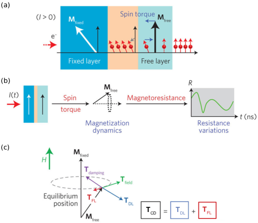
Figure 1: Spin-transfer torque basics: (a) in a ferromagnet/non-magnetic-spacer/ferromagnet setup, with noncollinear magnetizations $\mathbf{M}_{\mathrm{fixed}}$ of the fixed FM layer and $\mathbf{M}_{\mathrm{free}}$ of the free FM layer, the transverse spin component of the conduction electrons (red) polarized in the direction of $\mathbf{M}_{\mathrm{fixed}}$ is absorbed as they pass through the free layer, thereby generating a torque on $\mathbf{M}_{\mathrm{free}}$; (b) device applications of STT in (a) are based on torque-induced magnetization dynamics that is converted into resistance variations via the magnetoresistive effects; (c) torques on $\mathbf{M}_{\mathrm{free}}$ where field-like component of current-driven STT, $\mathbf{T}_{\mathrm{FL}}$, is orthogonal to the plane spanned by $\mathbf{M}_{\mathrm{fixed}}$ and $\mathbf{M}_{\mathrm{free}}$ and competes with the effective-field torque $\mathbf{T}_{\mathrm{field}}$ (present also in equilibrium), while damping-like component of current-driven STT, $\mathbf{T}_{\mathrm{DL}}$, is parallel or antiparallel (depending on the current direction) to Gilbert damping torque $\mathbf{T}_{\mathrm{damping}}$ (present also in equilibrium). The illustration in (c) assumes particular case where $\mathbf{M}_{\mathrm{fixed}}$ and the effective magnetic field are aligned. Adapted from Ref. Locatelli2014 .

Another setup exhibiting current-induced magnetization dynamics is illustrated in Figs. 2(b) and  2(c). It utilizes a single FM layer, so that the role of polarizing FM layer with $\mathbf{M}_{\mathrm{fixed}}$ in Figs. 1(a) and  2(a) is taken over by strong spin-orbit coupling (SOC) introduced by heavy metals (HMs) Miron2011 ; Liu2012c (such as $5d$ metals Pt, W and Ta) as in Fig. 2(b), topological insulators (TIs) Mellnik2014 ; Fan2014a ; Han2017 ; Wang2017 , Weyl semimetals (WSMs) MacNeill2017 ; MacNeill2017a , and even atomically thin transition metal dichalcogenides (TMDs) Sklenar2016 ; Shao2016 ; Guimaraes2018 ; Lv2018 . The TMDs are compounds of the type MX₂ (M = Mo, W, Nb; X = S, Se, Te) where one layer of M atoms is sandwiched between two layers of X atoms, as illustrated by monolayer MoS₂ in Fig. 2(c). The SOC is capable of converting charge into spin currents Vignale2010 ; Sinova2015 ; Soumyanarayanan2016 , so that their absorption by the FM layer in Figs. 2(b) and  2(c) leads to the so-called spin-orbit torque (SOT) Manchon2018 on its free magnetization $\mathbf{M}_{\mathrm{free}}$.

The current-driven (CD) STT and SOT vectors are analyzed by decomposing them into two contributions, $\mathbf{T}_{\mathrm{CD}}=\mathbf{T}_{\mathrm{DL}}+\mathbf{T}_{\mathrm{FL}}$, commonly termed Ralph2008 ; Manchon2018 damping-like (DL) and field-like (FL) torque based on how they enter into the LLG equation describing the classical dynamics of magnetization. As illustrated in Fig. 1(c), these two torque components provide two different handles to manipulate the dynamics of $\mathbf{M}_{\mathrm{free}}$. In the absence of current, displacing $\mathbf{M}_{\mathrm{free}}$ out of its equilibrium position leads to the effective-field torque $\mathbf{T}_{\mathrm{field}}$ which drives $\mathbf{M}_{\mathrm{free}}$ into precession around the effective magnetic field, while Gilbert damping $\mathbf{T}_{\mathrm{damping}}$ acts to bring it back to its equilibrium position. Under nonequilibrium conditions, brought by injecting steady-state or pulse current Baumgartner2017 , $\mathbf{T}_{\mathrm{DL}}$ acts opposite to $\mathbf{T}_{\mathrm{damping}}$ for “fixed-to-free” current direction and it enhances $\mathbf{T}_{\mathrm{damping}}$ for “free-to-fixed” current directions in Fig. 1(a). Thus, the former (latter) acts as antidamping (overdamping) torque trying to bring $\mathbf{M}_{\mathrm{free}}$ antiparallel (parallel) to $\mathbf{M}_{\mathrm{fixed}}$ (note that at cryogenic temperatures one finds apparently only antidamping action of $\mathbf{T}_{\mathrm{DL}}$ for both current directions Zholud2017 ). The $\mathbf{T}_{\mathrm{FL}}$ component induces magnetization precession and modifies the energy landscape seen by $\mathbf{M}_{\mathrm{free}}$. Although $|\mathbf{T}_{\mathrm{FL}}|$ is minuscule in metallic spin-valves Wang2008b , it can reach 30–40% of $|\mathbf{T}_{\mathrm{DL}}|$ in MTJs Sankey2008 ; Kubota2008 , and it can become several times larger than $|\mathbf{T}_{\mathrm{DL}}|$ in FM/HM bilayers Kim2013 ; Yoon2017 . Thus, $\mathbf{T}_{\mathrm{FL}}$ component of SOT can play a crucial role Baumgartner2017 ; Yoon2017 in triggering the reversal process of $\mathbf{M}_{\mathrm{free}}$ and in enhancing the switching efficiency. In concerted action with $\mathbf{T}_{\mathrm{DL}}$ and possible other effects brought by interfacial SOC, such as the Dzyaloshinskii-Moriya interaction Perez2014 , this can also lead to complex inhomogeneous magnetization switching patterns observed in SOT-operated devices Baumgartner2017 ; Yoon2017 ; Perez2014 .

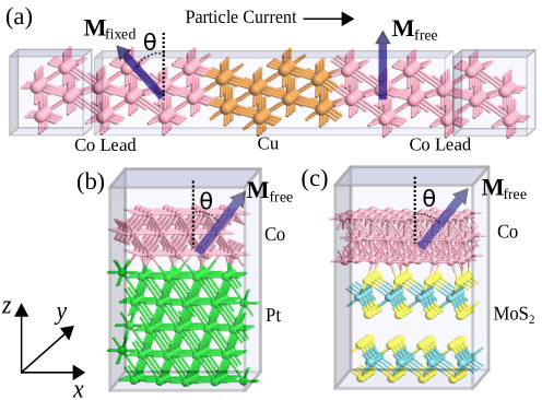
Figure 2: Schematic view of: (a) FM/NM/FM trilayer for calculations of STT in spin-valves; (b) FM/HM bilayer for calculations of SOT in the presence of the spin Hall current along the $z$-axis generated by the HM layer; and (c) FM/monolayer-TMD for calculations of SOT in the absence of any spin Hall current. The semi-infinite FM layers in (a) are chosen as Co(0001), and the spacer in between consists of $l$ ($l=4$ in the illustration) monolayers of Cu(111). The trilayer in (a) is assumed to be infinite in the transverse directions to the current flow, so that the depicted supercell is periodically repeated within the $yz$-plane. The bilayer in (b) consists of Co(0001) and Pt(111), and in (c) it consists of Co(0001) and monolayer MoS₂. The bilayers in (b) and (c) are assumed to be infinite in the $xy$-plane, but of finite thickness along the $z$-axis. Small bias voltage $V_{b}$ is applied to inject electrons along the positive $x$-axis, so that particle current is perpendicular to interfaces in (a) and parallel to the interface in (b) and (c).

By adjusting the ratio $|\mathbf{T}_{\mathrm{DL}}|/|\mathbf{T}_{\mathrm{FL}}|$ Timopheev2015 via tailoring of material properties and device shape, as well as by tuning the amplitude and duration of the injected pulse current Baumgartner2017 , both STT- and SOT-operated devices can implement variety of functionalities, such as: nonvolatile magnetic random access memories (MRAM) of almost unlimited endurance; microwave oscillators; microwave detectors; spin-wave emitters; memristors; and artificial neural networks Locatelli2014 ; Kent2015 ; Borders2017 . The key goal in all such applications is to actively manipulate magnetization dynamics, without the need for external magnetic fields that are incompatible with downscaling of the device size, while using the smallest possible current (e.g., writing currents $\lesssim 20$ $\mu$A would enable multigigabit MRAM Kent2015 ) and energy consumption. For example, recent experiments Wang2017 have demonstrated current-driven magnetization switching at room temperature in FM/TI bilayers using current density $\sim 10^{5}$ A/cm², which is two orders of magnitude smaller than for STT-induced magnetization switching in MTJs or one to two orders of magnitude smaller than for SOT-induced magnetization switching in FM/HM bilayers. The SOT-MRAM is expected to be less affected by damping, which offers flexibility for choosing the FM layer, while it eliminates insulating barrier in the writing process and its possible dielectric breakdown in STT-MRAM based on MTJs Kent2015 . Also, symmetric switching profile of SOT-MRAM evades the asymmetric switching issues in STT-MRAM otherwise requiring additional device/circuit engineering. On the other hand, SOT-MRAM has a disadvantage of being a three-terminal device.

II How to model spin torque using nonequilibrium density matrix combined with density functional theory calculations

The absorption of the component of flowing spin angular momentum that is transverse to $\mathbf{M}_{\mathrm{free}}$, as illustrated in Fig. 1(a), occurs Stiles2002 ; Wang2008b within a few ferromagnetic monolayers (MLs) near NM/FM or I/FM interface. Since the thickness of this interfacial region is typically shorter Wang2008b than any charge or spin dephasing length that would make electronic transport semiclassical, STT requires quantum transport modeling Brataas2006 . The essence of STT can be understood using simple one-dimensional (1D) models solved by matching spin-dependent wave function across the junction, akin to elementary quantum mechanics problems of transmission and reflection through a barrier, as provided in Refs. Ralph2008 ; Manchon2008a ; Xiao2008a . However, to describe details of experiments, such as bias voltage dependence of STT in MTJs Kubota2008 ; Sankey2008 or complex angular dependence of SOT in FM/HM bilayers Garello2013 , more involved calculations are needed employing tight-binding or first-principles Hamiltonian as an input. For example, simplistic tight-binding Hamiltonians (TBHs) with single orbital per site have been coupled Theodonis2006 to nonequilibrium Green’s function (NEGF) formalism Stefanucci2013 to compute SOT in FM/HM bilayers Kalitsov2017 , or bias voltage dependence of DL and FL components of STT in MTJs which can describe some features of the experiments by adjusting the tight-binding parameters Kubota2008 .

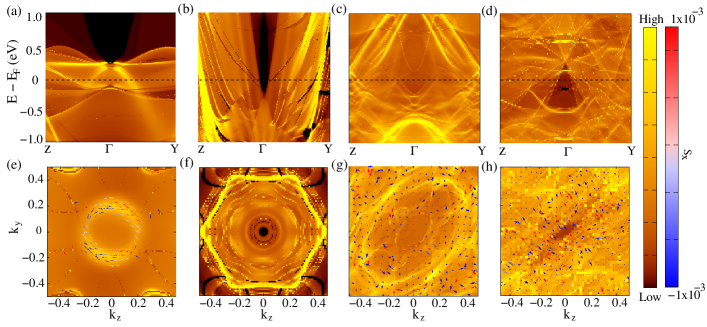
Figure 3: Spectral function $A(E;\mathbf{k}_{\parallel},x\in\mathrm{ML\ of\ Co})$, defined in Eq. (6), plotted along high symmetry $k$-path $Z$-$\Gamma$-$Y$ at: (a) the surface of semi-infinite Co(0001) in contact with vacuum; (b) ML of semi-infinite Co(0001) in contact with 9 MLs of Cu(111) within Co/Cu(9 ML)/Co spin-valve; (c) ML of semi-infinite Co(0001) in contact with 5 MLs of Pt(111); and (d) ML of semi-infinite Co(0001) in contact with 1 ML of MoS₂. Panels (e)–(h) plot constant energy contours of $A(E-E_{F}=0;\mathbf{k}_{\parallel},x\in\mathrm{ML\ of\ Co})$ and the corresponding spin textures where the out-of-plane $S_{x}$ component of spin is indicated in color (red for positive and blue for negative). The magnetization of Co is along the $x$-axis which is perpendicular to the ML of Co over which the spectral functions and spin textures are scanned. The units for $k_{y}$ and $k_{z}$ are $2\pi/a$ and $2\pi/b$ where $a$ and $b$ are the lattice constants along the $y$- and the $z$-axis, respectively. The horizontal dashed black line in panels (a)–(d) denotes the position of the Fermi energy $E_{F}$. Panels (a) and (e) are adapted from Ref. Marmolejo-Tejada2017 , and panels (c) and (g) are adapted from Ref. Dolui2017 .

However, not all features of STT experiments on MTJs Wang2011 can be captured by such NEGF+TBH approach. Furthermore, due to spin-orbit proximity effect, driven by hybridization of wave functions from FM and HM layers Dolui2017 or FM and metallic surfaces of three-dimensional (3D) TIs Marmolejo-Tejada2017 , simplistic Hamiltonians like the Rashba ferromagnetic model Manchon2008 ; Haney2013 ; Lee2015 ; Li2015 ; Pesin2012a ; Ado2017 ; Kalitsov2017 or the gapped Dirac model Ndiaye2017 are highly inadequate to describe realistic bilayers employed in SOT experiments. This is emphasized by Fig. 3 which shows how spectral function and spin texture on the surface of semi-infinite Co layer can change dramatically as we change the adjacent layer. For example, nonzero in-plane spin texture on the surface of semi-infinite Co layer in contact with vacuum is found in Fig. 3(e), despite Co magnetization being perpendicular to that surface. This is the consequence of the Rashba SOC enabled by inversion symmetry breaking Chantis2007 where an electrostatic potential gradient can be created by the charge distribution at the metal/vacuum interface to confine wave functions into a Rashba spin-split quasi two-dimensional (2D) electron gas Bahramy2012 . The surface of semi-infinite Co within layer embedded into Co/Cu(9 ML)/Co junction illustrated in Fig. 2(a) does not have any in-plane spin texture in Fig. 3(f) since the structure is inversion symmetric, but its spectral function in Fig. 3(b) is quite different from the one on the surface of an isolated semi-infinite Co layer in Fig. 3(a). Bringing semi-infinite Co layer in contact with 5 MLs of Pt or 1 ML of MoS₂ transforms its spectral function from Fig. 3(a) to the ones in Figs. 3(c) and  3(d), respectively, while inducing the corresponding spin textures in Figs. 3(g) and  3(h) due to spin-orbit proximity effect signified by the “leakage” of SOC from HM or TMD layer into the FM layer.

Note that the spectral function and spin texture at the Co/Pt interface are quite different from those of the ferromagnetic Rashba Hamiltonian in 2D often employed Manchon2008 ; Haney2013 ; Lee2015 ; Li2015 ; Pesin2012a ; Ado2017 ; Kalitsov2017 in the calculations of SOT as the putative simplistic description of the FM/HM interface. When charge current flows within FM monolayer hosting spin textures—such as the ones displayed in Figs. 3(e),  3(g) and 3(h)—more forward-going electron states will be occupied and less the backward going ones which due to spin-momentum locking leads to nonequilibrium spin density Edelstein1990 ; Aronov1989 as one of the principal mechanisms behind SOT Manchon2018 . The direction of the nonequilibrium spin density is easily identified in the case of simple spin textures, such as the one in Fig. 3(e) or those associated with simplistic models Pesin2012 like the Rashba Hamiltonian or the Dirac Hamiltonian discussed in Sec. IV. Conversely, for complex spin textures within heterostructures of realistic materials, as exemplified by those in Figs. 3(g) and  3(h), one needs first-principles coupled with electronic transport calculations Chang2015 ; Johansson2018 .

Thus, capturing properties of realistic junctions illustrated by Fig. 3 requires first-principles Hamiltonian as offered by the density functional theory (DFT). In the linear-response regime, appropriate for spin-valves or SOT-operated bilayers in Fig. 2, one can also employ first-principles derived TBH as offered by transforming the DFT Hamiltonian to a basis of orthogonal maximally localized Wannier functions (MLWFs) in a selected energy window around the Fermi energy $E_{F}$. This procedure retains faithfully the overlap matrix elements and their phases, orbital character of the bands and the accuracy of the original DFT calculations Marzari2012 . While Wannier TBH has been used to describe infinite-FM-on-infinite-HM bilayers Freimuth2014 ; Mahfouzi2018 , its accuracy can be compromised by complicated band entanglement in hybridized metallic systems Marzari2012 . It is also cumbersome to construct Wannier TBH for junctions in other geometries, like the spin-valve in Fig. 2(a) or when FM/HM bilayer is attached to leads made of different NM material. In such cases, one needs to perform multiple calculations Shelley2011 ; Thygesen2005a (such as on periodic leads, supercell composed of the central region of interest attached to buffer layers of the lead material on both sides, etc.) where one can encounter different MLWFs for two similar but nonidentical systems Thygesen2005a ; nonorthogonal MLWFs belonging to two different regions Thygesen2005a ; and Fermi energies of distinct calculations that have to be aligned Shelley2011 . Also, to compute current or STT in MTJs at finite bias voltage one needs to recalculate Hamiltonian in order to take into account self-consistent charge redistribution and the corresponding electrostatic potential in the presence of current flow. Otherwise, without computing them across the device the current-voltage characteristics violates Christen1996 ; Hernandez2013 gauge invariance, i.e., invariance with respect to the global shift of electric potential by a constant, $V\rightarrow V+V_{0}$.

The noncollinear DFT (ncDFT) Capelle2001 ; Eich2013a ; Eich2013 ; Bulik2013 coupled to nonequilibrium density matrix Stefanucci2013 offers an algorithm to compute spin torque in arbitrary device geometry at vanishing or finite bias voltage. The single-particle spin-dependent Kohn-Sham (KS) Hamiltonian in ncDFT takes the form

$$\hat{H}_{\mathrm{KS}}=-\frac{\hbar^{2}\nabla^{2}}{2m}+V_{\mathrm{H}}({\bf r})+V_{\rm XC}({\bf r})+V_{\rm ext}({\bf r})-{\bm{\sigma}}\cdot\mathbf{B}_{\mathrm{XC}}(\mathbf{r}),$$ (1)

where $V_{H}({\bf r})$, $V_{\rm ext}({\bf r})$ and $V_{\mathrm{XC}}({\bf r})=E_{\mathrm{XC}}[n(\mathbf{r}),\mathbf{m}(\mathbf{r})]/\delta n(\mathbf{r})$ are the Hartree, external and exchange-correlation (XC) potentials, respectively, and ${\bm{\sigma}}=(\hat{\sigma}_{x},\hat{\sigma}_{y},\hat{\sigma}_{z})$ is the vector of the Pauli matrices. The extension of DFT to the case of spin-polarized systems is formally derived in terms of total electron density $n(\mathbf{r})$ and vector magnetization density $\mathbf{m}(\mathbf{r})$. In the collinear DFT, $\mathbf{m}(\mathbf{r})$ points in the same direction at all points in space, which is insufficient to study magnetic systems where the direction of the local magnetization is not constrained to a particular axis or systems with SOC. In ncDFT Capelle2001 , XC functional $E_{\mathrm{XC}}[n(\mathbf{r}),\mathbf{m}(\mathbf{r})]$ depends on $\mathbf{m}(\mathbf{r})$ pointing in arbitrary direction. The XC magnetic field is then given by $\mathbf{B}_{\mathrm{XC}}(\mathbf{r})=\delta E_{\mathrm{XC}}[n(\mathbf{r}),\mathbf{m}(\mathbf{r})]/\delta\mathbf{m}(\mathbf{r})$.

Once the Hamiltonian of the device is selected, it has to be passed into the formalism of nonequilibrium quantum statistical mechanics. Its concept is the density matrix ${\bm{\rho}}$ of quantum many-particle system at finite temperature, or in the presence of external static or time-dependent fields which drive the system out of equilibrium. The knowledge of ${\bm{\rho}}$ makes it possible to compute the expectation value of any observable

$$O=\mathrm{Tr}\,[{\bm{\rho}}\mathbf{O}],$$ (2)

such as the charge density, charge current, spin current and spin density of interest to spin torque modeling. These requires to insert their operators (in some matrix representation) as $\mathbf{O}$ into Eq. (2), where we use notation in which bold letters denote matrix representation of an operator in a chosen basis. For the KS Hamiltonian in ncDFT in Eq. (1), the torque operator is given by the time derivative of the electronic spin operator Haney2007 ; Carva2009

$$\mathbf{T}=\frac{d{\bf S}}{dt}=\frac{1}{2i}[{\bm{\sigma}},\mathbf{H}_{\mathrm{KS}}]={\bm{\sigma}}\times\mathbf{B}_{\mathrm{XC}},$$ (3)

Its trace with ${\bm{\rho}}$ yields the spin torque vector while concurrently offering a microscopic picture Haney2007 for the origin of torque—misalignment of the nonequilibrium spin density of current carrying quasiparticles with respect to the spins of electrons comprising the magnetic condensate responsible for nonzero $\mathbf{B}_{\mathrm{XC}}$. This causes local torque on individual atoms, which is summed by performing trace in Eq. (2) to find the net effect on the total magnetization $\mathbf{M}_{\mathrm{free}}$ of the free FM layer. Examples of how to evaluate such trace, while using $\mathbf{O}\mapsto\mathbf{T}$ in Eq. (3) in different matrix representations, are given as Eqs. (25) and  (26) in Sec. III.

In equilibrium, ${\bm{\rho}}_{\mathrm{eq}}$ is fixed by the Boltzmann-Gibbs prescription, such as ${\bm{\rho}}_{\mathrm{eq}}=\sum_{n}f(E)|\Psi_{n}\rangle\langle\Psi_{n}|$ in grand canonical ensemble describing electrons with the Fermi distribution function $f(E)$ due to contact with a macroscopic reservoir at chemical potential $\mu$ and temperature $T$, where $E_{n}$ and $|\Psi_{n}\rangle$ are eigenenergies and eigenstates of the Hamiltonian, respectively. Out of equilibrium, the construction of ${\bm{\rho}}_{\mathrm{neq}}$ is complicated by the variety of possible driving fields and open nature of a driven quantum system. For example, the Kubo linear-response theory has been used to obtain ${\bm{\rho}}_{\mathrm{neq}}$ for small applied electric field in infinite-FM-on-infinite-HM bilayer geometry Freimuth2014 ; Mahfouzi2018 . However, for arbitrary junction geometry and magnitude of the applied bias voltage $V_{b}$ or injected pulse current, the most advantageous is to employ the NEGF formalism Stefanucci2013 . This requires to evaluate its two fundamental objects—the retarded GF, $G^{\sigma\sigma^{\prime}}_{\mathbf{nn}^{\prime}}(t,t^{\prime})=-i\Theta(t-t^{\prime})\langle\{\hat{c}_{\mathbf{n}\sigma}(t),\hat{c}^{\dagger}_{\mathbf{n}^{\prime}\sigma^{\prime}}(t^{\prime})\}\rangle$, and the lesser GF, $G^{<,\sigma\sigma^{\prime}}_{\mathbf{nn}^{\prime}}(t,t^{\prime})=i\langle\hat{c}^{\dagger}_{\mathbf{n}^{\prime}\sigma^{\prime}}(t^{\prime})\hat{c}_{\mathbf{n}\sigma}(t)\rangle$—describing the density of available quantum states and how electrons occupy those states, respectively. The operator $\hat{c}_{\mathbf{n}\sigma}^{\dagger}$ ($\hat{c}_{\mathbf{n}\sigma}$) creates (annihilates) electron with spin $\sigma$ at site $\mathbf{n}$ (another index would be required to label more than one orbital present at the site), and $\langle\ldots\rangle$ denotes the nonequilibrium statistical average Stefanucci2013 .

In time-dependent situations, the nonequilibrium density matrix is given by Petrovic2018 ; Stefanucci2013

$${\bm{\rho}}_{\mathrm{neq}}(t)=\mathbf{G}^{<}(t,t)/i.$$ (4)

In stationary problems $\mathbf{G}$ and $\mathbf{G}^{<}$ depend only on the time difference $t-t^{\prime}$ and can, therefore, be Fourier transformed to depend on energy $E$ instead of $t-t^{\prime}$. The retarded GF in stationary situations is then given by

$$\mathbf{G}(E)=\left[E-\mathbf{H}-{\bm{\Sigma}}_{L}(E,V_{b})-{\bm{\Sigma}}_{R}(E,V_{b})\right]^{-1},$$ (5)

assuming representation in the basis of orthogonal orbitals. In the case of nonorthogonal basis set $|\phi_{n}\rangle$, one should make a replacement $E\mapsto E\mathbf{S}$ where $\mathbf{S}$ is the overlap matrix composed of elements $\langle\phi_{n}|\phi_{m}\rangle$. The self-energies Velev2004 ; Rungger2008 ${\bm{\Sigma}}_{L,R}(E,V_{b})$ describe the semi-infinite leads which guarantee continuous energy spectrum of devices in Fig. 2 required to reach the steady-state transport regime. The leads terminate at infinity into the left (L) and right (R) macroscopic reservoirs with different electrochemical potentials, $\mu_{L}-\mu_{R}=eV_{L}-eV_{R}=eV_{b}$. The usual assumption about the leads is that the applied bias voltage $V_{b}$ induces a rigid shift in their electronic structureBrandbyge2002 , so that ${\bm{\Sigma}}_{L,R}(E,V_{b})={\bm{\Sigma}}_{L,R}(E-eV_{L,R})$.

In equilibrium or near equilibrium (i.e., in the linear-response transport regime at small $eV_{b}\ll E_{F}$), one needs $\mathbf{G}_{0}(E)$ obtained from Eq. (5) by setting $V_{L}=V_{R}=0$. The spectral functions shown in Fig. 3(a)–(d) can be computed at an arbitrary plane at position $x$ within the junction in Fig. 2(a) using $\mathbf{G}_{0}(E)$

$$A(E;\mathbf{k}_{\parallel},x)=-\frac{1}{\pi}\mathrm{Im}\,[G_{0}(E;{\mathbf{k}_{\parallel}};x,x)],$$ (6)

where the diagonal matrix elements $G_{0}(E;{\mathbf{k}_{\parallel}};x,x)$ are obtained by transforming the retarded GF from a local orbital to a real-space representation. The spin textures in Fig. 3(e)–(h) within the constant energy contours are computed from the spin-resolved spectral function. The equilibrium density matrix can also be expressed in terms of $\mathbf{G}_{0}(E)$

$${\bm{\rho}}_{\mathrm{eq}}=-\frac{1}{\pi}\int\limits_{-\infty}^{+\infty}dE\,{\rm Im}\,\mathbf{G}_{0}(E)f(E),$$ (7)

where $\mathrm{Im}\,\mathbf{O}=(\mathbf{O}-\mathbf{O}^{\dagger})/2i$.

The nonequilibrium density matrix is determined by the lesser GF

$${\bm{\rho}}_{\mathrm{neq}}=\frac{1}{2\pi i}\int\limits_{-\infty}^{+\infty}dE\,\mathbf{G}^{<}(E).$$ (8)

In general, if a quantity has nonzero expectation values in equilibrium, that one must be subtracted from the final result since it is unobservable in transport experiments. This is exemplified by spin current density in time-reversal invariant systems Nikolic2006 ; spin density, diamagnetic circulating currents and circulating heat currents in the presence of external magnetic field or spontaneous magnetization breaking time-reversal invariance; and FL component of STT Theodonis2006 . Thus, we define the current-driven part of the nonequilibrium density matrix as

$${\bm{\rho}}_{\mathrm{CD}}={\bm{\rho}}_{\mathrm{neq}}-{\bm{\rho}}_{\mathrm{eq}}.$$ (9)

Although the NEGF formalism can include many-body interactions, such as electron-magnon scattering Mahfouzi2014 that can affect STT Zholud2017 ; Levy2006 ; Manchon2010 and SOT Yasuda2017 ; Okuma2017 , here we focus on the usually considered and conceptually simpler elastic transport regime where the lesser GF of a two-terminal junction

$$\mathbf{G}^{<}(E)=\mathbf{G}(E)\left[if_{L}(E){\bm{\Gamma}}_{L}(E)+if_{R}(E){\bm{\Gamma}}_{R}(E)\right]\mathbf{G}^{\dagger}(E),$$ (10)

is expressed solely in terms of the retarded GF, the level broadening matrices ${\bm{\Gamma}}_{L,R}(E)=i[{\bm{\Sigma}}_{L,R}(E)-{\bm{\Sigma}}_{L,R}^{\dagger}(E)]$ determining the escape rates of electrons into the semi-infinite leads and shifted Fermi functions $f_{L,R}(E)=f(E-eV_{L,R})$.

For purely computational purposes, the integration in Eq. (8) is typically separated (non-uniquely Xie2016 ) into the apparent “equilibrium” and current-driven “nonequilibrium” terms Brandbyge2002 ; Sanvito2011

$${\bm{\rho}}_{\mathrm{neq}}=-\frac{1}{\pi}\int\limits_{-\infty}^{+\infty}dE\,{\rm Im}\,\mathbf{G}(E)f(E-eV_{R})+\frac{1}{2\pi}\int\limits_{-\infty}^{+\infty}dE\,\mathbf{G}(E)\cdot{\bm{\Gamma}}_{L}(E-eV_{L})\cdot\mathbf{G}^{\dagger}(E)\left[f_{L}(E)-f_{R}(E)\right].$$ (11)

The first “equilibrium” term contains integrand which is analytic in the upper complex plane and can be computed via contour integration Brandbyge2002 ; Areshkin2010 ; Ozaki2007 ; Karrasch2010 , while the integrand in the second “current-driven” term is nonanalytic function in the entire complex energy plane so that its integration has to be performed directly along the real axis Sanvito2011 between the limits set by the window of nonzero values of $f_{L}(E)-f_{R}(E)$. Although the second term in Eq. (11) contains information about the bias voltage [through the difference $f_{L}(E)-f_{R}(E)$] and about the lead assumed to be injecting electrons into the device (through ${\bm{\Gamma}}_{L}$), it cannot Xie2016 ; Mahfouzi2013 be used as the proper ${\bm{\rho}}_{\mathrm{CD}}$ defined in Eq. (9). This is due to the fact that second term in Eq. (9), expressed in terms of the retarded GF via Eq. (7), does not cancel the gauge-noninvariant first term in Eq. (11) which depends explicitly [through $f(E-eV_{R})$] on the arbitrarily chosen reference potential $V_{R}$ and implicitly on the voltages applied to both reservoirs [through $\mathbf{G}(E)$]. Nevertheless, the second term in Eq. (11), written in the linear-response and zero-temperature limit,

$${\bm{\rho}}_{\mathrm{CD}}\stackrel{{\scriptstyle?}}{{=}}\frac{eV_{b}}{2\pi}\mathbf{G}_{0}(E_{F})\cdot{\bm{\Gamma}}_{L}(E_{F})\cdot\mathbf{G}_{0}^{\dagger}(E_{F}),$$ (12)

has often been used in STT literature Haney2007 ; Heiliger2008b as the putative but improper (due to being gauge-noninvariant, which we mark by using “?” on the top of the equality sign) expression for ${\bm{\rho}}_{\rm CD}$. Its usage leads to ambiguous (i.e., dependent on arbitrarily chosen $V_{R}$) nonequilibrium expectation values.

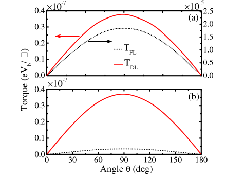
Figure 4: The angular dependence of the damping-like (i.e., parallel), $|\mathbf{T}_{\mathrm{DL}}|$, and field-like (i.e., perpendicular), $|\mathbf{T}_{\mathrm{FL}}|$, components of the STT vector in Fig. 1(c) in an asymmetric Oh2009 FM/I/FM^′ MTJ computed in the linear-response regime at zero-temperature using: (a) the proper gauge-invariant expression Eq. (13) for ${\bm{\rho}}_{\mathrm{CD}}$; and (b) the improper gauge-noninvariant expression Eq. (12) for ${\bm{\rho}}_{\mathrm{CD}}$. The FM/I/FM^′ trilayer in Fig. 1(a) is modeled by TBH Theodonis2006 defined on an infinite cubic lattice with a single orbital per site and lattice spacing $a$. Its insulating barrier has thickness 5 MLs with on-site potential $\varepsilon_{n}=6.0$ eV; the left FM layer is semi-infinite and the right FM^′ layer is 20 MLs thick. Both FM layers have the same exchange field $J=0.5$ eV. The symbol $\Box=a^{2}$ denotes unit interfacial area. Adapted from Ref. Mahfouzi2013 .

The proper gauge invariant expressions was derived in Ref. Mahfouzi2013

$${\bm{\rho}}_{\rm CD}=\frac{eV_{b}}{2\pi}\mathbf{G}_{0}(E_{F})\cdot{\bm{\Gamma}}_{L}(E_{F})\cdot\mathbf{G}_{0}^{\dagger}(E_{F})-\frac{eV_{R}}{\pi}\mathrm{Im}\,\mathbf{G}_{0}(E_{F})-\frac{1}{\pi}\int\limits_{-\infty}^{+\infty}\!\!dE\,\mathrm{Im}\left[\mathbf{G}_{0}\left(eU_{\mathbf{n}}-eV_{L}\frac{\partial{\bm{\Sigma}}_{L}}{\partial E}-eV_{R}\frac{\partial{\bm{\Sigma}}_{R}}{\partial E}\right)\mathbf{G}_{0}\right]f(E),$$ (13)

which we give here at zero-temperature so that it can be contrasted with Eq. (12). The second and third term in Eq. (13), whose purpose is to subtract any nonzero expectation value that exists in thermodynamic equilibrium, make it quite different from Eq. (12) while requiring to include also electrostatic potential profile $U_{\mathbf{n}}$ across the active region of the device interpolating between $V_{L}$ and $V_{R}$. For example, the second term in Eq. (13) traced with an operator gives equilibrium expectation value governed by the states at $E_{F}$ which must be removed. The third term in Eq. (13) ensures the gauge invariance of the nonequilibrium expectation values, while making the whole expression non-Fermi-surface property. The third term also renders the usage of Eq. (13) computationally demanding due to the requirement to perform integration from the bottom of the band up to $E_{F}$ together with sampling of $\mathbf{k}_{\parallel}$ points for the junctions in Fig. 2.

In Fig. 4 we consider an example of a left-right asymmetric MTJ, FM/I/FM^′, whose FM and FM^′ layers are assumed to be made of the same material but have different thicknesses. This setup allows us to demonstrate how application of improper ${\bm{\rho}}_{\rm CD}$ in Eq. (12) yields linear-response ${\bf T}_{\mathrm{FL}}\propto V_{b}$ in Fig. 4(b) that is incorrectly an order of magnitude smaller than the correct result in Fig. 4(a). This is due to the fact that ${\bf T}_{\mathrm{FL}}$ in MTJs posses both the nonequilibrium CD contribution due to spin reorientation at interfaces, where net spin created at one interface is reflected at the second interface where it briefly precesses in the exchange field of the free FM layer, and equilibrium contribution due to interlayer exchange coupling Theodonis2006 ; Yang2010 . The ambiguity in Fig. 4 arises when this equilibrium contribution is improperly subtracted, so that current-driven ${\bf T}_{\mathrm{FL}}$ in Fig. 4(b) is contaminated by a portion of equilibrium contribution added to it when using improper ${\bm{\rho}}_{\mathrm{CD}}$ in Eq. (12). On the other hand, since ${\bf T}_{\mathrm{DL}}$ has a zero expectation value in equilibrium, both the proper and improper expressions for ${\bm{\rho}}_{\mathrm{CD}}$ give the same result in Fig. 4.

Note that in the left-right symmetric MTJs, $\mathbf{T}_{\mathrm{FL}}\propto V_{b}$ vanishes. Since this is a rather general result which holds for both MTJs and spin-valves in the linear-response regime Theodonis2006 ; Xiao2008a ; Heiliger2008 , and it been confirmed in numerous experiments Wang2011 ; Oh2009 , one can use it as a validation test of the computational scheme. For example, the usage of improper ${\bm{\rho}}_{\mathrm{CD}}$ in Eq. (12), or the proper one in Eq. (13) but with possible software bug, would give nonzero ${\bf T}_{\mathrm{FL}}\neq 0$ in symmetric junctions at small applied $V_{b}$ which contradicts experiments Wang2011 ; Oh2009 . In the particular case of symmetric junction one can actually employ a simpler expression Mahfouzi2013 ; Stamenova2017 than Eq. (13) which guarantees ${\bf T}_{\mathrm{FL}}\equiv 0$

$${\bm{\rho}}_{\mathrm{CD}}=\frac{eV_{b}}{4\pi}\mathbf{G}_{0}(E_{F})\cdot[{\bm{\Gamma}}_{L}(E_{F})-{\bm{\Gamma}}_{R}(E_{F})]\cdot\mathbf{G}_{0}^{\dagger}(E_{F}),$$ (14)

obtained by assuming Mahfouzi2013 the particular gauge $V_{L}=-V_{b}/2=-V_{R}$. Such special gauges and the corresponding Fermi surface expressions for ${\bm{\rho}}_{\mathrm{CD}}\propto V_{b}$ in the linear-response regime do exist also for asymmetric junctions, but one does not know them in advance except for the special case of symmetric junctions Mahfouzi2013 .

In the calculations in Fig. 4, we first compute $(T^{x}_{\mathrm{CD}},T^{y}_{\mathrm{CD}},T^{z}_{\mathrm{CD}})=\mathrm{Tr}\,[{\bm{\rho}}_{\rm CD}\mathbf{T}]$ using the torque operator $\mathbf{T}$ akin to Eq. (3) but determined by the TBH of the free FM layer. These three numbers are then used to obtain FL (or perpendicular) torque component, $T_{\mathrm{FL}}=T^{y}_{\mathrm{CD}}$ along the direction $\mathbf{M}_{\mathrm{free}}\times\mathbf{M}_{\mathrm{fixed}}$, and DL (or parallel) torque component, $T_{\mathrm{DL}}=\sqrt{(T^{x}_{\mathrm{CD}})^{2}+(T^{z}_{\mathrm{CD}})^{2}}$ in the direction $\mathbf{M}_{\mathrm{free}}\times(\mathbf{M}_{\mathrm{free}}\times\mathbf{M}_{\mathrm{fixed}})$. In MTJs angular dependence of STT components stems only from the cross product, so that $\propto\sin\theta$ dependence Theodonis2006 ; Xiao2008a for both FL and DL components in obtained in Figs. 4 and  5.

In the case of SOT, $\mathbf{T}_{\mathrm{DL}}\propto\mathbf{M}_{\mathrm{free}}\times\mathbf{f}$ and $\mathbf{T}_{\mathrm{DL}}\propto\mathbf{M}_{\mathrm{free}}\times(\mathbf{M}_{\mathrm{free}}\times\mathbf{f})$, where the direction specified by the unit vector $\mathbf{f}$ is determined dynamically once the current flows in the presence of SOC. Therefore, $\mathbf{f}$ is not known in advance (aside from simplistic models like the Rashba ferromagnetic one where $\mathbf{f}$ is along the $y$-axis for charge current flowing along the $x$-axis, as illustrated in Fig. 9). Thus, it would be advantageous to decompose ${\bm{\rho}}_{\mathrm{CD}}$ into contributions whose trace with the torque operator in Eq. (3) directly yield $\mathbf{T}_{\mathrm{DL}}$ and $\mathbf{T}_{\mathrm{FL}}$. Such decomposition was achieved in Ref. Mahfouzi2016 , using adiabatic expansion of Eq. (4) in the powers of $d\mathbf{M}_{\mathrm{free}}/dt$ and symmetry arguments, where ${\bm{\rho}}_{\mathrm{neq}}={\bm{\rho}}_{\mathrm{neq}}^{\mathrm{oo}}+{\bm{\rho}}_{\mathrm{neq}}^{\mathrm{oe}}+{\bm{\rho}}_{\mathrm{neq}}^{\mathrm{eo}}+{\bm{\rho}}_{\mathrm{neq}}^{\mathrm{ee}}$ is the sum of the following terms

$${\bm{\rho}}^{\mathrm{oo}}_{\mathrm{neq}} = \frac{1}{8\pi}\int\limits_{-\infty}^{+\infty}dE\,\left[f_{L}(E)-f_{R}(E)\right]\left(\mathbf{G}{\bm{\Gamma}}_{L}\mathbf{G}^{\dagger}-\mathbf{G}^{\dagger}{\bm{\Gamma}}_{L}\mathbf{G}-\mathbf{G}{\bm{\Gamma}}_{R}\mathbf{G}^{\dagger}+\mathbf{G}^{\dagger}{\bm{\Gamma}}_{R}\mathbf{G}\right),$$ (15)

$${\bm{\rho}}^{\mathrm{oe}}_{\mathrm{neq}} = \frac{1}{8\pi}\int\limits_{-\infty}^{+\infty}dE\,\left[f_{L}(E)-f_{R}(E)\right]\left(\mathbf{G}{\bm{\Gamma}}_{L}\mathbf{G}^{\dagger}+\mathbf{G}^{\dagger}{\bm{\Gamma}}_{L}\mathbf{G}-\mathbf{G}{\bm{\Gamma}}_{R}\mathbf{G}^{\dagger}-\mathbf{G}^{\dagger}{\bm{\Gamma}}_{R}\mathbf{G}\right),$$ (16)

$${\bm{\rho}}^{\mathrm{eo}}_{\mathrm{neq}} = \frac{1}{8\pi}\int\limits_{-\infty}^{+\infty}dE\,\left[f_{L}(E)+f_{R}(E)\right]\left(\mathbf{G}{\bm{\Gamma}}_{L}\mathbf{G}^{\dagger}-\mathbf{G}^{\dagger}{\bm{\Gamma}}_{L}\mathbf{G}+\mathbf{G}{\bm{\Gamma}}_{R}\mathbf{G}^{\dagger}-\mathbf{G}^{\dagger}{\bm{\Gamma}}_{R}\mathbf{G}\right)\equiv 0,$$ (17)

$${\bm{\rho}}^{\mathrm{ee}}_{\mathrm{neq}} = \frac{1}{8\pi}\int\limits_{-\infty}^{+\infty}dE\,\left[f_{L}(E)+f_{R}(E)\right]\left(\mathbf{G}{\bm{\Gamma}}_{L}\mathbf{G}^{\dagger}+\mathbf{G}^{\dagger}{\bm{\Gamma}}_{L}\mathbf{G}+\mathbf{G}{\bm{\Gamma}}_{R}\mathbf{G}^{\dagger}+\mathbf{G}^{\dagger}{\bm{\Gamma}}_{R}\mathbf{G}\right).$$ (18)

The four terms are labeled by being odd (o) or even (e) under inverting bias polarity (first index) or time (second index) Mahfouzi2016 . The terms ${\bm{\rho}}^{\mathrm{oo}}_{\mathrm{neq}}$ and ${\bm{\rho}}^{\mathrm{oe}}_{\mathrm{neq}}$ depend on $f_{L}(E)-f_{R}(E)$ and, therefore, are nonzero only in nonequilibrium generated by the bias voltage $V_{b}\neq 0$ which drives the steady-state current. Using an identity from the NEGF formalism Stefanucci2013 , $\mathbf{G}({\bm{\Gamma}}_{L}+{\bm{\Gamma}_{R}})\mathbf{G}^{\dagger}=i(\mathbf{G}-\mathbf{G}^{\dagger})$, reveals that ${\bm{\rho}}^{\mathrm{eo}}_{\mathrm{neq}}\equiv 0$ and

$${\bm{\rho}}^{\mathrm{ee}}_{\mathrm{neq}}=-\frac{1}{2\pi}\int\limits_{-\infty}^{+\infty}dE\,[f_{L}(E)+f_{R}(E)]\mathrm{Im}\,\mathbf{G}.$$ (19)

Thus, ${\bm{\rho}}^{\mathrm{ee}}_{\mathrm{neq}}$ term is nonzero even in equilibrium where it becomes identical to the equilibrium density matrix in Eq. (7), $V_{b}=0\Rightarrow{\bm{\rho}}^{\mathrm{ee}}_{\mathrm{neq}}\equiv{\bm{\rho}}_{\mathrm{eq}}$. Since ${\bm{\rho}}^{\mathrm{oo}}_{\mathrm{neq}}$ is odd under time reversal, its trace with the torque operator in Eq. (3) yields DL component of STT (which depends on three magnetization vectors and it is, therefore, also odd) and FL component of SOT (which depends on one magnetization vectors and it is, therefore, also odd). Similarly trace of ${\bm{\rho}}^{\mathrm{oe}}_{\mathrm{neq}}$ with the torque operator in Eq. (3) yields FL component of STT and DL component of SOT Mahfouzi2016 .

In the linear-response regime, pertinent to calculations of STT in spin-valves and SOT in FM/spin-orbit-coupled-material bilayers, $f_{L}(E)-f_{R}(E)\rightarrow(-\partial f/\partial E)eV_{b}$. This confines integration in ${\bm{\rho}}^{\mathrm{oo}}_{\mathrm{neq}}$ and ${\bm{\rho}}^{\mathrm{oe}}_{\mathrm{neq}}$ expressions to a shell of few $k_{B}T$ around the Fermi energy, or at zero temperature these are just matrix products evaluated at the Fermi energy, akin to Eqs. (12),  (13) and  (14). Nevertheless, to obtain ${\bm{\rho}}_{\mathrm{CD}}={\bm{\rho}}_{\mathrm{neq}}^{\mathrm{oo}}+{\bm{\rho}}_{\mathrm{neq}}^{\mathrm{oe}}+{\bm{\rho}}_{\mathrm{neq}}^{\mathrm{eo}}+{\bm{\rho}}_{\mathrm{neq}}^{\mathrm{ee}}-{\bm{\rho}}_{\mathrm{eq}}$ one still needs to perform the integration over the Fermi sea in order to obtain ${\bm{\rho}}_{\mathrm{neq}}^{\mathrm{ee}}-{\bm{\rho}}_{\mathrm{eq}}$, akin to Eq. (13), which can be equivalently computed as $[{\bm{\rho}}_{\mathrm{neq}}^{\mathrm{ee}}(V_{b})-{\bm{\rho}}_{\mathrm{neq}}^{\mathrm{ee}}(-V_{b})]/2$ using some small $V_{b}$.

To evade singularities on the real axis caused by the poles of the retarded GF in the matrix integral of the type $\int\limits_{-\infty}^{+\infty}dE\,\mathbf{G}f_{p}(E)$ appearing in Eqs. (7), (13) and (19), such integration can be performed along the contour in the upper half of the complex plane where the retarded GF is analytic. The widely used contour Brandbyge2002 consists of a semicircle, a semi-infinite line segment and a finite number of poles of the Fermi function $f_{p}(E)$. This contour should be positioned sufficiently far away from the real axis, so that $\mathbf{G}$ is smooth over both of these two segments, while also requiring to select the minimum energy $E_{\mathrm{min}}$ (as the starting point of semicircular path) below the bottom of the band edge which is not known in advance in DFT calculations. That is, in self-consistent calculations, incorrectly selected minimum energy causes charge to erroneously disappear from the system with convergence trivially achieved but to physically incorrect solution. By choosing different types of contours Areshkin2010 ; Ozaki2007 ; Karrasch2010 (such as the “Ozaki contour” Ozaki2007 ; Karrasch2010 we employ in the calculations in Fig. 9) where residue theorem leads to just a sum over a finite set of complex energies, proper positioning of $E_{\mathrm{min}}$ and convergence in the number of Fermi poles, as well as selection of sufficient number of contour points along the semicircle and contour points on the line segment are completely bypassed.

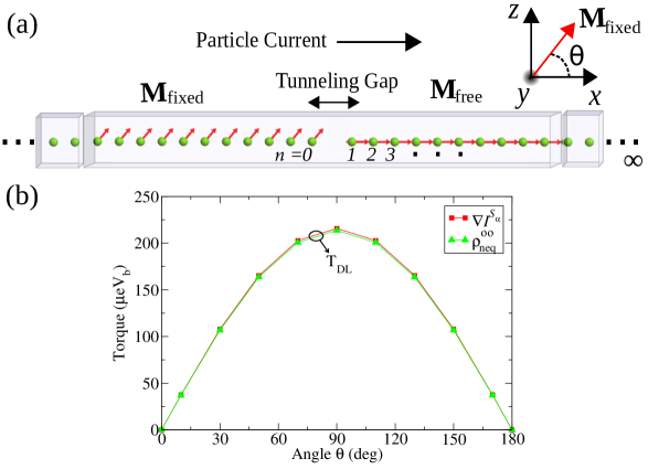
Figure 5: (a) Schematic view of a 1D toy model of MTJ consisting of the left and the right semi-infinite chains of carbon atoms separated by a vacuum gap. (b) Comparison of DL component of STT in this MTJ computed via the spin current divergence algorithm Theodonis2006 ; Wang2008b in Eq. (20) and by using decomposition of the nonequilibrium density matrix into ${\bm{\rho}}_{\mathrm{neq}}^{\mu\nu}$ contributions in Eqs. (15)–(19). The DL component of STT, computed in both algorithms in the linear-response regime, acts on the right carbon chain whose magnetic moments comprise the free magnetization $\mathbf{M}_{\mathrm{free}}$ rotated by an angle $\theta$ with respect to the fixed magnetization $\mathbf{M}_{\mathrm{fixed}}$ of the left carbon chain. Since MTJ is left-right symmetric, the FL component of the STT vector is zero in the linear-response regime Wang2011 ; Theodonis2006 ; Xiao2008a ; Oh2009 ; Heiliger2008 .

Prior to application of the algorithm based on Eqs. (15)–(19) to STT calculations in Sec. III and SOT calculations in Sec. IV, we compare it to often employed spin current divergence algorithm Theodonis2006 ; Wang2008b ; Manchon2008a using a toy model of 1D MTJ. The model, illustrated in Fig. 5(a) where the left and right semi-infinite chains of carbon atoms are separated by a vacuum gap, is described by the collinear DFT Hamiltonian implemented in ATK package atk using single-zeta polarized Junquera2001 orbitals on each atom, Ceperly-Alder Ceperley1980 parametrization of the local spin density approximation for the XC functional Ceperley1980 and norm-conserving pseudopotentials accounting for electron-core interactions. In the absence of spin-flip processes by impurities and magnons or SOC, the STT vector at site $n$ within the right chain can be computed from the divergence (in discrete form) of spin current Theodonis2006 , $T_{n}^{\alpha}=-\nabla I^{S_{\alpha}}=I_{n-1,n}^{S_{\alpha}}-I_{n,n+1}^{S_{\alpha}}$. Its sum over the whole free FM layer gives the total STT as

$$T^{\alpha}_{\mathrm{CD}}=\sum_{n=1}^{N_{\mathrm{free}}}(I_{n-1,n}^{S_{\alpha}}-I_{n,n+1}^{S_{\alpha}})=I_{0,1}^{S_{\alpha}}-I_{N_{\mathrm{free}},N_{\mathrm{free}}+1}^{S_{\alpha}}.$$ (20)

Here $I_{0,1}^{S_{\alpha}}$ is the local spin current, carrying spins pointing in the direction $\alpha\in\{x,y,z\}$, from the last site inside the barrier [which is the last site of the left carbon chain in Fig. 5(a)] toward the first site of the free FM layer [which is the first site of the right carbon chain in Fig. 5(a)]. Similarly, $I_{N_{\mathrm{free}},N_{\mathrm{free}}+1}$ is the local spin current from the last site inside the free FM layer and the first site of the right lead. Thus, Eq. (20) expresses STT on the free FM layer composed of $N_{\mathrm{free}}$ sites as the difference Wang2008b between spin currents entering through its left and exiting through its right interface. In the case of semi-infinite free FM layer, $N_{\mathrm{free}}\rightarrow\infty$ and $I_{N_{\mathrm{free}},N_{\mathrm{free}}+1}\rightarrow 0$. The nonequilibrium local spin current can be computed in different ways Wang2008b , one of which utilizes NEGF expression for ${\bm{\rho}}_{\mathrm{CD}}$

$$I_{n,n+1}^{S_{\alpha}}=\frac{i}{2}\mathrm{Tr}\,\left[{\bm{\sigma}}_{\alpha}\left(\mathbf{H}_{n,n+1}{\bm{\rho}}_{\mathrm{CD}}^{n+1,n}-{\bm{\rho}}_{\mathrm{CD}}^{n,n+1}\mathbf{H}_{n+1,n}\right)\right].$$ (21)

Here $\mathbf{H}_{n,n+1}$ and ${\bm{\rho}}_{\mathrm{CD}}^{n,n+1}$ are the submatrices of the Hamiltonian and the current-driven part of the nonequilibrium density matrix, respectively, of the size $2N_{\mathrm{orbital}}\times 2N_{\mathrm{orbital}}$ (2 is for spin and $N_{\mathrm{orbital}}$ is for the number of orbitals per each atom) which connect sites $n$ and $n+1$.

Combining Eqs. (14),  (20) and  (21) yields $T^{x}_{\mathrm{CD}}$ and $T^{z}_{\mathrm{CD}}$ from which we obtain $T_{\mathrm{DL}}=\sqrt{(T^{x}_{\mathrm{CD}})^{2}+(T^{z}_{\mathrm{CD}})^{2}}$ in the linear-response regime plotted in Fig. 5(b) as a function of angle $\theta$ between $\mathbf{M}_{\mathrm{free}}$ and $\mathbf{M}_{\mathrm{fixed}}$. Alternatively, evaluating the trace of the product of ${\bm{\rho}}_{\mathrm{neq}}^{\mathrm{oo}}$ and the torque operator in Eq. (3) yields a vector with two nonzero components, which turn out to be identical to $T^{x}_{\mathrm{CD}}$ and $T^{z}_{\mathrm{CD}}$ computed from the spin current divergence algorithm, as demonstrated in Fig. 5(b). The trace of ${\bm{\rho}}_{\mathrm{neq}}^{\mathrm{oe}}$ with the torque operator gives a vector with zero $x$- and $z$-components and nonzero $y$-component which, however, is canceled by adding the trace of ${\bm{\rho}}_{\mathrm{neq}}^{\mathrm{ee}}-{\bm{\rho}}_{\mathrm{eq}}$ with the torque operator to finally produce zero FL component of the STT vector. This is expected because MTJ in Fig. 5(a) is left-right symmetric.

We emphasize that the algorithm based on the trace of the torque operator with the current-driven part of the nonequilibrium density matrix $\mathbf{\bm{\rho}}_{\mathrm{CD}}$ is a more general approach than the spin current divergence algorithm since it is valid even in the presence of spin-flip processes by impurities and magnons or SOC Haney2007 . In particular, it can be employed to compute SOT Freimuth2014 ; Mahfouzi2018 in FM/spin-orbit-coupled-material bilayers where spin torque cannot Haney2010 be expressed any more as in Eq. (20).

III Example: Spin-transfer torque in FM/NM/FM trilayer spin-valve structures

First-principles quantum transport modeling of STT in spin-valves Haney2007 ; Wang2008b and MTJs Stamenova2017 ; Heiliger2008 ; Jia2011 ; Ellis2017 is typically conducted using an assumption that greatly simplifies computation—noncollinear spins in such systems are described in a rigid approximation where one starts from the collinear DFT Hamiltonian and then rotates magnetic moments of either fixed or free FM layer in the spin space in order to generate the relative angle between $\mathbf{M}_{\mathrm{fixed}}$ and $\mathbf{M}_{\mathrm{free}}$ (as it was also done in the calculations of STT in 1D toy model of MTJ in Fig. 5). On the other hand, obtaining true ground state of such system requires noncollinear XC functionals Capelle2001 ; Eich2013a ; Eich2013 ; Bulik2013 and the corresponding self-consistent XC magnetic field $\mathbf{B}_{\mathrm{xc}}$ introduced in Eq. (1). For a given self-consistently converged ncDFT Hamiltonian represented in the linear combination of atomic orbitals (LCAO) basis, we can extract the matrix representation of $\mathbf{B}_{\mathrm{xc}}^{\alpha}$ in the same basis using

$$\mathbf{B}_{\mathrm{XC}}^{x} = 2\cdot{\rm Re}\,\mathbf{H}^{\uparrow\downarrow},$$ (22)

$$\mathbf{B}_{\mathrm{XC}}^{y} = -2\cdot{\rm Im}\,\mathbf{H}^{\uparrow\downarrow},$$ (23)

$$\mathbf{B}_{\mathrm{XC}}^{z} = \mathbf{H}^{\uparrow\uparrow}-\mathbf{H}^{\downarrow\downarrow}.$$ (24)

Since LCAO basis sets $|\phi_{n}\rangle$ are typically nonorthogonal (as is the case of the basis sets Junquera2001 ; Ozaki2003 ; Schlipf2015 implemented in ATK atk and OpenMX openmx packages we employ in the calculations of Figs. 5–8), the trace leading to the spin torque vector

$$\mathbf{T}_{\mathrm{CD}}=\mathrm{Tr}\,[{\bm{\rho}}_{\mathrm{CD}}{\bm{\sigma}}\times\mathbf{S}^{-1}\mathbf{B}_{\mathrm{XC}}],$$ (25)

requires to use the identity operator $\mathbf{1}=\sum_{ij}|\phi_{i}\rangle S_{ij}^{-1}\langle\phi_{j}|$ which inserts $\mathbf{S}^{-1}$ matrix into Eq. (25) where all matrices inside the trace are representations in the LCAO basis. In the real-space basis spanned by the eigenstates $|\mathbf{r}\rangle$ of the position operator, the same trace in Eq. (25) becomes

$$\mathbf{T}_{\mathrm{CD}}=\int\limits_{\mathrm{free\ FM}}\!\!\!d^{3}\mathbf{r}\,\mathbf{m}_{\mathrm{CD}}(\mathbf{r})\times\mathbf{B}_{\mathrm{XC}}(\mathbf{r}).$$ (26)

This is a nonequilibrium generalization of the equilibrium torque expression found in ncDFT Capelle2001 —effectively, $\mathbf{m}_{\mathrm{eq}}(\mathbf{r})=\langle\mathbf{r}|{\bm{\rho}}_{\mathrm{eq}}{\bm{\sigma}}|\mathbf{r}\rangle$ in ncDFT is replaced by $\mathbf{m}_{\mathrm{CD}}(\mathbf{r})=\langle\mathbf{r}|{\bm{\rho}}_{\mathrm{CD}}{\bm{\sigma}}|\mathbf{r}\rangle$. Note that in thermodynamic equilibrium integral in Eq. (26) must be zero when integration is performed over all space, which is denoted as “zero-torque theorem” Capelle2001 , but $\mathbf{m}_{\mathrm{eq}}\times\mathbf{B}_{\mathrm{XC}}(\mathbf{r})$ can be nonzero locally which gives rise to equilibrium torque on the free FM layer that has to be removed by subtracting ${\bm{\rho}}_{\mathrm{eq}}$ to obtain ${\bm{\rho}}_{\mathrm{CD}}$ in Eq. (9) and plug it into Eq. (26).

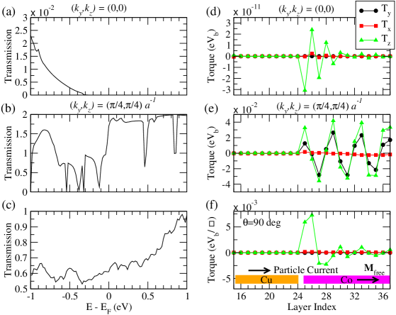
Figure 6: (a),(b) Transmission function, defined in Eq. (27), for Co/Cu(9 ML)/Co spin-valve illustrated in Fig. 2(a) at two selected transverse wave vectors $\mathbf{k}_{\parallel}$; as well as (c) summed, as in Eq. (28), over all $\mathbf{k}_{\parallel}$ vectors within the 2D BZ. (d)–(f) The corresponding layer-resolved Cartesian components of the STT vector at an angle $\theta=90^{\circ}$ between the magnetizations $\mathbf{M}_{\mathrm{fixed}}$ of the left Co layer acting as a polarizer and $\mathbf{M}_{\mathrm{free}}$ of the right Co layer receiving the torque. The mesh of $\mathbf{k}_{\parallel}$ equally spaced points employed in (c) is $51\times 51$, and in (f) it is $201\times 201$. The symbol $\Box=a^{2}$ denotes unit interfacial area, where $a=2.52$ Å is the lattice constant of a common 2D hexagonal unit cell of Co/Cu bilayer (with a lattice mismatch of about 0.65%).

We employ ATK package to compute STT in Co/Cu(9 ML)/Co spin-valve illustrated in Fig. 2(a) using ncDFT Hamiltonian combined with Eq. (25). Prior to DFT calculations, we employ the interface builder in the VNL package vnl to construct a common unit cell for Co/Cu bilayer. In order to determine the interlayer distance and relaxed atomic coordinates, we perform DFT calculations using VASP vasp ; Kresse1993 ; Kresse1996a with Perdew-Burke-Ernzerhof (PBE) parametrization Perdew1996 of the generalized gradient approximation for the XC functional and projected augmented wave Blochl1994 ; Kresse1999 description of electron-core interactions. The cutoff energy for the plane wave basis set is chosen as 600 eV, while $k$-points were sampled on a $11\times 11$ surface mesh. In ATK calculations we use PBE XC functional, norm-conserving pseudopotentials for describing electron-core interactions and SG15 (medium) LCAO basis set Schlipf2015 . The energy mesh cut-off for the real-space grid is chosen as 100 Hartree.

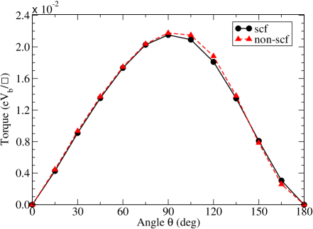
Figure 7: The DL component of STT vector in symmetric Co/Cu(9 ML)/Co spin-valve in Fig. 2(a) driven by current at small bias voltage $V_{b}$ as a function of angle $\theta$ between the magnetizations $\mathbf{M}_{\mathrm{fixed}}$ of the left Co layer and $\mathbf{M}_{\mathrm{free}}$ of the right Co layer. Its value at $\theta=90^{\circ}$ is the sum of layer-resolved STT shown in Fig. 6(f). The non-scf curve is computed from Eq. (25) using the rigid approximation Haney2007 ; Wang2008b ; Heiliger2008 ; Jia2011 , where spin-valve is described by collinear DFT Hamiltonian and magnetic moments of the fixed Co layer are rotated by an angle theta with respect to magnetic moments in the free Co layer. Conversely, in the computation of scf curve, the DFT Hamiltonian from the rigid approximation serves as the first iteration leading toward converged self-consistent ncDFT Hamiltonian of the spin-valve.

The layer-resolved Cartesian components of STT vector within the free Co layer are shown in Fig. 6(d)–(f). The contribution from a propagating state oscillates as a function of position without decaying in Fig. 6(e) with a spatial period $2\pi/(k^{\downarrow}_{\zeta}-k^{\uparrow}_{\eta})$ where $\zeta$ ($\eta$) denotes different sheets Wang2008b of the Fermi surface for minority (majority) spin. This is due to the fact that noncollinear spin in Fig. 2 entering right Co layer is not an eigenstate of the spin part of the Hamiltonian determined by $\mathbf{M}_{\mathrm{free}}$ and it is, therefore, forced into precession. However, since the shapes of the Fermi surface for majority and minority spin in Co are quite different from each other Wang2008b , the spatial periods of precession can vary rapidly for different $\mathbf{k}_{\parallel}$ within the 2D Brillouin zone (BZ). Thus, summation of their contributions leads to cancellation and, therefore, fast decay of STT away from the interface Stiles2002 ; Wang2008b , as demonstrated by plotting such sum to obtain the total STT per ML of Co in Fig. 6(f).

The propagating vs. evanescent states are identified by finite [Fig. 6(b)] vs. vanishing [Fig. 6(a)], respectively, $\mathbf{k}_{\parallel}$-resolved transmission function obtained from the Landauer formula in terms of NEGFs Stefanucci2013

$$T(E,\mathbf{k}_{\parallel})=\mathrm{Tr}\,[{\bm{\Gamma}}_{R}(E,\mathbf{k}_{\parallel})\mathbf{G}_{0}(E,\mathbf{k}_{\parallel}){\bm{\Gamma}}_{L}(E,\mathbf{k}_{\parallel})\mathbf{G}_{0}^{\dagger}(E,\mathbf{k}_{\parallel})],$$ (27)

where the transverse wave vector $\mathbf{k}_{\parallel}$ is conserved in the absence of disorder. The total transmission function per unit interfacial area is then evaluated using ($\Omega_{\mathrm{BZ}}$ is the area of sampled 2D BZ)

$$T(E)=\frac{1}{\Omega_{\mathrm{BZ}}}\int\limits_{\mathrm{2D\ BZ}}T(E,\mathbf{k}_{\parallel}),$$ (28)

as shown in Fig. 6(c). The transmission function in Fig. 6(a) at $\mathbf{k}_{\parallel}=(0,0)$ vanishes at the Fermi energy, signifying evanescent state which cannot carry any current across the junction. Nonetheless, such states can contribute Ralph2008 ; Stiles2002 ; Wang2008b to STT vector, as shown in Fig. 6(d). Thus, the decay of STT away from Cu/Co interface in Fig. 6(f) arises both from the cancellation among contributions from propagating states with different $\mathbf{k}_{\parallel}$ and the decay of contributions from each evanescent state, where the latter are estimated Wang2008b to generate $\simeq 10$% of the total torque on the ML of free Co layer that is closest to the Cu/Co interface in Fig. 2(a).

Since the considered Co/Cu(9 ML)/Co spin-valve is left-right symmetric, the FL component of the STT vector is zero. The DL component, as the sum of all layer-resolved torques in Fig. 6(f), is plotted as a function of the relative angle $\theta$ between $\mathbf{M}_{\mathrm{fixed}}$ and $\mathbf{M}_{\mathrm{free}}$ in Fig. 7. The angular dependence of STT in spin-valves does not follow $\propto\sin\theta$ dependence found in the case of MTJs in Figs. 4 and  5.

Although similar analyses have been performed before using collinear DFT Hamiltonian and rigid rotation of magnetic moments in fixed Co layer Haney2007 ; Wang2008b , in Fig. 7 we additionally quantify an error made in this approximation by computing torque using ncDFT Hamiltonian. The rigid approximation is then just the first iteration of the full self-consistent field (scf) calculations leading to our converged ncDFT Hamiltonian. The difference between scf and non-scf calculations in Fig. 7 is rather small due to large number of spacer MLs of Cu, but it could become sizable for small number of spacer MLs enabling coupling between two FM layers.

IV Example: Spin-orbit torque in FM/monolayer-TMD bilayers

The calculation of SOT driven by injection of unpolarized charge current into bilayers of the type FM/HM shown in Fig. 2(b); FM/monolayer-TMD shown in Fig. 2(c); FM/TI; or FM/WSM can be performed using the same NEGF+ncDFT framework combining the torque operator $\mathbf{T}$, ${\bm{\rho}}_{\mathrm{CD}}$ expressed in terms of NEGFs and ncDFT Hamiltonian that was delineated in Sec. II and applied in Sec. III to compute the STT vector in spin-valves. Such first-principles quantum transport approach can also easily accommodate possible third capping insulating layer (such as MgO or AlO_x) employed experimentally to increase Kim2013 the perpendicular magnetic anisotropy which tilts magnetization out of the plane of the interface. However, the results of such calculations are not as easy to interpret as in the case of a transparent picture Stiles2002 ; Wang2008b in Fig. 6(d)–(f) explaining how spin angular momentum gets absorbed close to the interface in junctions which exhibit conventional STT. This is due to the fact that several microscopic mechanisms can contribute to SOT, such as: the spin Hall effect (SHE) Vignale2010 ; Sinova2015 within the HM layer Freimuth2014 ; Mahfouzi2018 with strong bulk SOC and around FM/HM interface Wang2016a ; current-driven nonequilibrium spin density—the so-called Edelstein effect Edelstein1990 ; Aronov1989 —due to strong interfacial SOC; spin currents generated in transmission and reflection from SO-coupled interfaces within 3D transport geometry Zhang2015 ; Kim2017 ; and spin-dependent scattering off impurities Pesin2012a ; Ado2017 or boundaries Mahfouzi2016 in the presence of SOC within FM monolayers. This makes it difficult to understand how to optimize SOT by tailoring materials combination or device geometry to enhance one or more of these mechanisms.

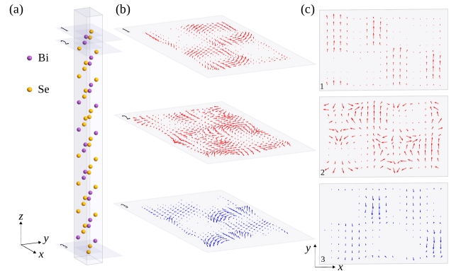
Figure 8: (a) The arrangement of Bi and Se atoms within a supercell of Bi₂Se₃ thin film (infinite in the $x$- and the $y$-directions) consisting of five quintuple layers (one such layer contains three Se layers strongly bonded to two Bi layers in between) and total thickness $\approx 5$ nm. (b) The vector field of current-driven nonequilibrium spin density $\mathbf{S}_{\mathrm{CD}}(\mathbf{r})$ within selected planes shown in (a), generated by injection of unpolarized charge current along the $x$-axis. The planes 1 and 3 correspond to the top and bottom metallic surfaces of Bi₂Se₃ thin film, while plane 2 resides in the bulk at a distance $d\approx 0.164$ nm away from plane 1. (c) The vector fields in (b) projected onto each of the selected planes in (a). The real space grid of points in panels (b) and (c) has spacing $\simeq 0.4$ Å. Adapted from Ref. Chang2015 .

An example of first-principles quantum transport modeling of the Edelstein effect is shown in Fig. 8 for the case of the metallic surface of Bi₂Se₃ as the prototypical 3D TI Bansil2016 . Such materials possess a usual band gap in the bulk, akin to conventional topologically trivial insulators, but they also host metallic surfaces whose low-energy quasiparticles behave as massless Dirac fermions. The spins of such fermions are perfectly locked to their momenta by strong SOC, thereby forming spin textures in the reciprocal-space Bansil2016 . In general, when charge current flows through a surface or interface with SOC, the presence of SOC-generated spin texture in the reciprocal-space, such as those shown in Figs. 3(e),  3(g) and  3(h), will generate nonequilibrium spin density which can be computed using

$$\mathbf{S}_{\mathrm{CD}}=\frac{\hbar}{2}\mathrm{Tr}\,[{\bm{\rho}}_{\mathrm{CD}}{\bm{\sigma}}].$$ (29)

In the case of simplistic Hamiltonians—such as the Rashba one for 2D electron gas Winkler2003 , $\hat{H}_{\mathrm{Rashba}}=(\hat{p}_{x}^{2}+\hat{p}_{y}^{2})/2m^{*}+\frac{\alpha_{\mathrm{SO}}}{\hbar}(\hat{\sigma}_{x}\hat{p_{y}}-\hat{\sigma}_{y}\hat{p_{x}})$, or the Dirac one for the metallic surface of 3D TI, $\hat{H}_{\mathrm{Dirac}}=v_{F}(\hat{\sigma}_{x}\hat{p_{y}}-\hat{\sigma}_{y}\hat{p_{x}})$—the direction and the magnitude of $\mathbf{S}_{\mathrm{CD}}$ are easily determined by back-of-the-envelope calculations Pesin2012 . For example, spin texture (i.e., expectation value of the spin operator in the eigenstates of a Hamiltonian) associated with $\hat{H}_{\mathrm{Rashba}}$ consists of spin vectors locked to momentum vector along the two Fermi circles formed in the reciprocal-space at the intersection of the Rashba energy-momentum dispersion Winkler2003 and the Fermi energy plane. Thus, current flow will disturb balance of momenta to produce $\mathbf{S}_{\mathrm{CD}}$ in the direction transverse to current flow. The same effect is substantially enhanced Pesin2012 , by a factor $\hbar v_{F}/\alpha_{\mathrm{SO}}\gg 1$ where $v_{F}$ is the Fermi velocity in TI and $\alpha_{\mathrm{SO}}$ is the strength of the Rashba SOC, because spin texture associated with $\hat{H}_{\mathrm{Dirac}}$ consists of spin vectors locked to momentum vector along a single Fermi circle formed in the reciprocal-space at the intersection of the Dirac cone energy-momentum dispersion Bansil2016 and the Fermi energy plane. This eliminates the compensating effect of the spins along the second circle in the case of $\hat{H}_{\mathrm{Rashba}}$. Note that nonzero total $\mathbf{S}_{\mathrm{CD}}\propto V_{b}$ generated by the Edelstein effect is allowed only in nonequilibrium since in equilibrium $\mathbf{S}$ changes sign under time reversal, and, therefore, has to vanish (assuming absence of external magnetic field or magnetization).

In the case of a thin film of Bi₂Se₃ described by ncDFT Hamiltonian, unpolarized injected charge current generates $\mathbf{S}_{\mathrm{CD}}=(0,S^{y}_{\mathrm{CD}},S^{z}_{\mathrm{CD}})$ on the top surface of the TI, marked as plane 1 in Fig. 8, where the in-plane component $S^{y}_{\mathrm{CD}}$ is an order of magnitude larger than the ouf-of-plane component $S^{z}_{\mathrm{CD}}$ arising due to hexagonal warping Bansil2016 of the Dirac cone on the TI surface. The spin texture on the bottom surface of the TI, marked as plane 3 in Fig. 8, has opposite sign to that shown on the top surface because of opposite direction of spins wounding along single Fermi circle on the bottom surface. In addition, a more complicated spin texture in real space (on a grid of points with $\simeq 0.4$ Å spacing), akin to noncollinear intra-atomic magnetism Nordstroem1996 but driven here by current flow, emerges within $\simeq 2$ nm thick layer below the TI surfaces. This is due to the penetration of evanescent wave functions from the metallic surfaces into the bulk of the TI, as shown in Fig. 8 by plotting $\mathbf{S}_{\mathrm{CD}}(\mathbf{r})$ within plane 2.

The conventional unpolarized charge current injected into the HM layer in Fig. 2(b) along the $x$-axis generates transverse spin Hall currents Vignale2010 ; Sinova2015 ; Wang2016a due to strong SOC in such layers. In 3D geometry, spin Hall current along the $y$-axis carries spins polarized along the $z$-axis, while the spin Hall current along the $z$-axis carries spins polarized along the $y$-axis Wang2016a . Thus, the effect of the spin Hall current flowing along the $z$-axis and entering FM layer resembles STT that would be generated by a fictitious polarizing FM layer with fixed magnetization along the $y$-axis and with charge current injected along the $z$-axis. While this mechanism is considered to play a major role in the generation of the DL component of SOT Liu2012c , as apparently confirmed by the Kubo-formula+ncDFT modeling Freimuth2014 ; Mahfouzi2018 , the product of signs of the FL and DL torque components is negative in virtually all experiments Yoon2017 (except for specific thicknesses of HM=Ta Kim2013 layer). Although HM layer in Fig. 2(b) certainly generates spin Hall current in its bulk, such spin current can be largely suppressed by the spin memory loss Dolui2017 ; Belashchenko2016 as electron traverses HM/FM interface with strong SOC. Thus, in contrast to positive sign product in widely accepted picture where SHE is most responsible for the DL component of SOT and Edelstein effect is most responsible for the FL component of SOT, negative sign product indicates that a single dominant mechanism could be responsible for both DL and FL torque.

In order to explore how such single mechanism could arise in the absence of spin Hall current, one can calculate torque in a number of specially crafted setups, such as the one chosen in Fig. 9(a) where we consider a single ultrathin FM layer (consisting of 4 or 10 MLs) with the Rashba SOC present either only in the bottom ML [marked as 0 in Fig. 9(a)] or in all MLs but with decreasing strength to mimic the spin-orbit proximity effect exemplified in Figs. 3(g) and  3(h). The setup in Fig. 9(a) is motivated by SOT experiments Sklenar2016 ; Shao2016 ; Guimaraes2018 ; Lv2018 on FM/monolayer-TMD heterostructures where SHE in absent due to atomically thin spin-orbit-coupled material. In such bilayers, clean and atomically precise interfaces have been achieved while back-gate voltage Lv2018 has been employed to demonstrate control of the ratio between the FL and DL components of SOT. Note that when bulk TMD or its even-layer thin films are centrosymmetric, its monolayer will be noncentrosymmetric crystal which results in lifting of the spin degeneracy and possibly strong SOC effects Zhu2011a .

In order to be able to controllably switch SOC on and off in different MLs, or to add other types of single-particle interactions, we describe setup in Fig. 9(a) using TBH defined on an infinite cubic lattice of spacing $a$ with a single orbital per site located at position $\mathbf{n}=(n_{x}a,n_{z}a)$

$$\hat{H}=\sum_{\mathbf{n}}\varepsilon_{\mathbf{n}}\hat{c}^{\dagger}_{\mathbf{n}}\hat{c}_{\mathbf{n}}+\sum_{\langle\mathbf{n}\mathbf{n}^{\prime}\rangle}\left(\hat{c}^{\dagger}_{\mathbf{n}}\mathbf{t}_{\mathbf{n}\mathbf{n}^{\prime}}\hat{c}_{\mathbf{n^{\prime}}}+{\rm h.c.}\right)-J\sum_{\mathbf{n}}\hat{c}^{\dagger}_{\mathbf{n}}\mathbf{M}_{\mathrm{free}}\cdot{\bm{\sigma}}\hat{c}_{\mathbf{n}}.$$ (30)

Here $\hat{c}_{\mathbf{n}}^{\dagger}=(\hat{c}^{\dagger}_{\mathbf{n}\uparrow}\ \ \hat{c}^{\dagger}_{\mathbf{n}\downarrow})$ is the row vector of operators which create electron at site $\mathbf{n}$ in spin-$\uparrow$ or spin-$\downarrow$ state, and $\hat{c}_{\mathbf{n}}=(\hat{c}_{\mathbf{n}\uparrow}\ \ \hat{c}_{\mathbf{n}\downarrow})$ is the column vector of the corresponding annihilation operators. The spin-dependent nearest-neighbor hoppings in the $xz$-plane form a $2\times 2$ matrix in the spin space

$$\mathbf{t}_{\mathbf{n}\mathbf{n}^{\prime}}=\left\{\begin{array}[]{ll}-t\otimes I_{2},&{\rm for}\ \ \mathbf{n}=\mathbf{n}^{\prime}+{\bm{e}}_{z},\\ -t\otimes I_{2}-i\gamma_{\rm SO}\sigma_{y},&{\rm for}\ \ \mathbf{n}=\mathbf{n}^{\prime}+{\bm{e}}_{x},\\ \end{array}\right.$$ (31)

where $\gamma_{\mathrm{SO}}=\alpha_{\mathrm{SO}}/2a$ measures the strength of the Rashba SOC on the lattice Nikolic2006 , $I_{2}$ is unit $2\times 2$ matrix and $\mathbf{e}_{\alpha}$ are the unit vectors along the axes of the Cartesian coordinate system. The on-site energy

$$\varepsilon_{\mathbf{n}}=\left[U_{\mathbf{n}}-2t\cos(k_{y}a\right)]\otimes I_{2}-2\gamma_{\rm SO}\sigma_{x}\sin(k_{y}a),$$ (32)

includes the on-site potential energy $U_{\mathbf{n}}$ (due to impurities, insulating barrier, voltage drop, etc.), as well as kinetic energy effectively generated by the periodic boundary conditions along the $y$-axis which simulate infinite extension of the FM layer in this direction and require $k_{y}$-point sampling in all calculations. The infinite extension along the $x$-axis is taken into account by splitting the device in Fig. 9(a) into semi-infinite left lead, central region of arbitrary length along the $x$-axis, and semi-infinite right lead, all of which are described by the Hamiltonian in Eq. (30) with the same values for $t=1$ eV, $J=0.1$ eV and the $\gamma_{\mathrm{SO}}$ chosen in all three regions. Thus, $\gamma_{\mathrm{SO}}$ is homogeneous within a given ML, and always present $\gamma_{\mathrm{SO}}=0.2$ eV on layer 0, but it can take different values in other MLs. The Fermi energy is set at $E_{F}=1.0$ eV to take into account possible noncircular Fermi surface Lee2015 effects in realistic materials.

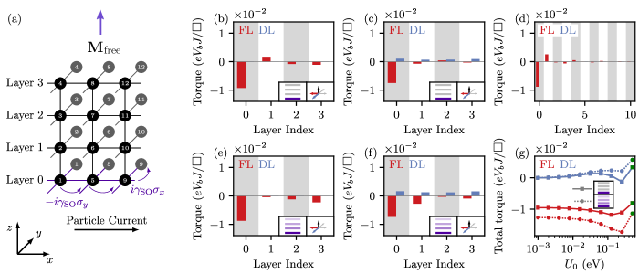
Figure 9: (a) Schematic view of an ultrathin FM layer comprised of few MLs, modeled as infinite square tight-binding lattices (with lattice constant $a$) in the $xy$-plane. The bottom layer 0 is assumed to be in direct contact with a spin-orbit-coupled material like TMD. (b)—(g) The layer-resolved FL and DL components of SOT vector per unit area $\Box=a^{2}$ for the device in (a) where FM film is 4 MLs thick in all panels except (d) where the thickness is 10 MLs. The bottom layer 0 is assumed to host the Rashba SOC of strength $\gamma_{\mathrm{SO}}=0.2$ eV, induced by the spin-orbit proximity effect from monolayer-TMD (which is assumed to be insulating and, therefore, not explicitly considered), as illustrated in Fig. 3(h) for Co/monolayer-MoS₂. This is twice as strong as the exchange field in the FM layer, $\gamma_{\mathrm{SO}}/J=2$ in Eq. (30). In panels (e) and (f) we also add the Rashba SOC in layers $l>0$ with strength 50% smaller than in layer $l-1$ (i.e., $\gamma_{\mathrm{SO}}=0.2$ eV, $0.1$ eV, $0.05$ eV and $0.025$ eV in layers 0–3, respectively). Panel (g) plots FL and DL components of SOT summed over all layers as a function of the strength of a homogeneous on-site potential $U_{\mathbf{n}}=U_{0}$ in Eq. (32) added into the central region of the thickness of 5 sites along the $x$-axis. The green square and dot in panel (g) mark SOT components at $U_{0}=0.5$ eV whose layer resolved values are shown in panels (c) and (f), respectively. The temperature is set at $T=300$ K, Fermi energy is $E_{F}=1$ eV and we use a grid of $N_{k_{y}}=2000$ equally spaced $k_{y}$-points to sample periodically repeated lattice in the $y$-direction. The red and blue arrows in the insets of panels (b),(c),(e) and (f) denote $\mathbf{M}_{\mathrm{free}}\times\mathbf{e}_{y}$ and $\mathbf{M}_{\mathrm{free}}\times(\mathbf{M}_{\mathrm{free}}\times\mathbf{e}_{y})$ unit vectors along the direction of FL and DL components of SOT, respectively. The quad-graphs in the insets of panels (b), (c), (e), (f) and (g) signify presence or absence of the Rashba SOC within layers 0–3 using the shade of the corresponding line.

The SOT is often studied Manchon2008 ; Haney2013 ; Lee2015 ; Li2015 ; Pesin2012a ; Ado2017 ; Kalitsov2017 using the Rashba ferromagnetic model in 2D, which corresponds to just a single layer in Fig. 9(a). In that case, only FL torque component is found Manchon2008 ; Kalitsov2017 due to the Edelstein effect, and in the absence of spin-dependent disorder Pesin2012a ; Ado2017 . This is also confirmed is our 3D transport geometry in Figs. 9(b),  9(d) and  9(e) where SOT vector, $\frac{2J}{\hbar}\mathbf{S}_{\mathrm{CD}}\times\mathbf{M}_{\mathrm{free}}$, on layer 0 has only FL component pointing in the $\mathbf{M}_{\mathrm{free}}\times\mathbf{e}_{y}$ direction, as long as the device is infinite clean and homogeneous. In addition, we also find nonzero FL component of SOT in Figs. 9(b) and  9(d) on layers above layer 0 despite that fact that only layer 0 hosts $\gamma_{\mathrm{SO}}\neq 0$. This is due to vertical transport along the $z$-axis in 3D geometry of Fig. 9(a), but in the absence of the Rashba SOC on other layers such effect decays fast as we move toward the top layer, as shown in Fig. 9(d) for 10 MLs thick FM film. The presence of the Rashba SOC with decreasing $\gamma_{\mathrm{SO}}$ on MLs above layer 0 generates additional nonequilibrium spin density $\mathbf{S}_{\mathrm{CD}}\propto\mathbf{e}_{y}$ on those layers and the corresponding enhancement of the FL component of SOT on those layers in  9(e).

We note that the Kubo-Bastin formula Bastin1971 adapted for SOT calculations Freimuth2014 predicts actually nonzero DL component of SOT vector for the Rashba ferromagnetic model in 2D due to change of electronic wave functions induced by an applied electric field termed the “Berry curvature mechanism” Lee2015 ; Kurebayashi2014 ; Li2015 . Despite being apparently intrinsic, i.e., insensitive to disorder, this mechanism can be completely canceled in specific models when the vertex corrections are taken into account Ado2017 . It also gives positive sign product Lee2015 ; Li2015 of DL and FL components of SOT contrary to majority of experiments where such product is found to be negative Yoon2017 . We emphasize that no electric field can exist in the ballistic transport regime through clean devices we analyze in Figs. 9(b),  9(d) and  9(e), for which the Kubo-Bastin formula also predicts unphysical divergence Freimuth2014 ; Mahfouzi2018 ; Lee2015 ; Kurebayashi2014 ; Li2015 of the FL component of SOT. Adding finite voltage drop within the central region, which is actually unjustified in the case of infinite clean homogeneous device, results in nonzero DL component of SOT also in the NEGF calculations Kalitsov2017 . However, the same outcome can be obtained simply by introducing constant potential $U_{\mathbf{n}}=U_{0}$ on each site of the central region acting as a barrier which reflects incoming electrons, as demonstrated in Figs. 9(c),  9(f) and  9(g). In the presence of both SOC and such barrier, spin-dependent scattering Pesin2012a ; Ado2017 is generated at the lead/central-region boundary which results in nonzero component of $\mathbf{S}_{\mathrm{CD}}$ in the direction $\mathbf{M}_{\mathrm{free}}\times\mathbf{e}_{y}$ and the corresponding DL component of SOT $\propto\mathbf{M}_{\mathrm{free}}\times(\mathbf{M}_{\mathrm{free}}\times\mathbf{e}_{y})$ acting on edge magnetic moments Mahfouzi2016 . This will, therefore, induce inhomogeneous magnetization switching which starts from the edges and propagates into the bulk of FM layer, as observed in experiments Baumgartner2017 and micromagnetic simulations Baumgartner2017 ; Mikuszeit2015 .

Interestingly, Fig. 9(g) also demonstrates that the signs of the DL and FL component are opposite to each other for almost all values of $U_{\mathbf{n}}=U_{0}$ (except when $U_{0}\simeq J$), as observed in majority of SOT experiments Yoon2017 . Importantly, the spin-orbit proximity effect within the MLs of FM layer close to FM/spin-orbit-coupled-material interface, as illustrated in Figs. 3(g) and  3(h) and mimicked by introducing the Rashba SOC of decaying strength within all MLs of FM thin film in Fig. 9(a), enhances both FL and DL components of SOT. This is demonstrated by comparing solid ($\gamma_{\mathrm{SO}}\neq 0$ only on layer 0) and dashed ($\gamma_{\mathrm{SO}}\neq 0$ on all layers 0–3) lines in Fig. 9(g). This points out at a knob that can be exploited to enhance SOT by searching for optimal combination of materials capable to generate penetration of SOC over long distances within the FM layer Marmolejo-Tejada2017 . In fact, in the case of FM/TI and FM/monolayer-TMD heterostructures, proximity SOC coupling within the FM layer is crucial for SOT efficiency Wang2017 where it has been considered Mellnik2014 that applied current will be shunted through the metallic FM layer and, therefore, not contribute to nonequilibrium spin density generation at the interface where SOC and thereby induced in-plane spin textures are naively assumed to reside.

V Conclusions

This Chapter reviews a unified first-principles quantum transport approach, implemented by combining NEGF formalism with ncDFT calculations, to compute both STT in traditional magnetic multilayers with two FM layers (i.e., the polarizing and analyzing FM layers with fixed and free magnetizations, respectively) and SOT in magnetic bilayers where only one of the layers is ferromagnetic. In the latter case, the role of the fixed magnetization of the polarizing FM layer within spin-valves or MTJs is taken over by the current-driven nonequilibrium spin density in the presence of strong SOC introduced by the second layer made of HM, 3D TI, WSM or monolayer-TMD. Our approach resolves recent confusion Freimuth2014 ; Kalitsov2017 in the literature where apparently only the Kubo formula, operating with expressions that integrate over the Fermi sea in order to capture change of wave functions due to the applied electric field and the corresponding interband electronic transitions Freimuth2014 ; Lee2015 ; Li2015 , can properly obtain the DL component of SOT. In addition, although the Kubo formula approach can also be integrated with first-principles calculations Freimuth2014 ; Mahfouzi2018 , it can only be applied to a single device geometry (where infinite FM layer covers infinite spin-orbit-coupled-material layer while current flows parallel to their interface) and in the linear-response transport regime. In contrast, NEGF+ncDFT approach reviewed in this Chapter can handle arbitrary device geometry, such as spin-valves and MTJs exhibiting STT or bilayers of the type FM/spin-orbit-coupled-material which are made inhomogeneous by attachment to NM leads, at vanishing or finite applied bias voltage. In contrast to often employed 2D transport geometry Manchon2008 ; Haney2013 ; Lee2015 ; Li2015 ; Pesin2012a ; Ado2017 ; Kalitsov2017 ; Ndiaye2017 for SOT theoretical analyses, we emphasize the importance of 3D transport geometry Kim2017 ; Ghosh2018 to capture both the effects at the FM/spin-orbit-coupled-material interface and those further into the bulk of the FM layer. Finally, ultrathin FM layers employed in SOT experiments can hybridize strongly with the adjacent spin-orbit-coupled-material to acquire its SOC and the corresponding spin textures on all of the FM monolayers. Such “hybridized ferromagnetic metals” can have electronic and spin structure (Fig. 3) which is quite different from an isolated FM layer, thereby requiring usage of both 3D geometry and first-principles Hamiltonians (of either tight-binding Freimuth2014 ; Mahfouzi2018 or pseudopotential-LCAO-ncDFT Theurich2001 type) to predict the strength of SOT in realistic systems and optimal materials combinations for device applications of the SOT phenomenon.

- (1) D. Ralph and M. Stiles, Spin transfer torques, J. Magn. Magn. Mater. 320, 1190 (2008).
- (2) N. Locatelli, V. Cros, and J. Grollier, Spin-torque building blocks, Nat. Mater. 13, 11 (2014).
- (3) J. C. Slonczewski, Current-driven excitation of magnetic multilayers, J. Magn. Magn. Mater. 159, L1 (1996).
- (4) L. Berger, Emission of spin waves by a magnetic multilayer traversed by a current, Phys. Rev. B 54, 9353 (1996).
- (5) M. Tsoi, A. G. M. Jansen, J. Bass, W.-C. Chiang, M. Seck, V. Tsoi, and P. Wyder, Excitation of a magnetic multilayer by an electric current, Phys. Rev. Lett. 80, 4281 (1998).
- (6) E. B. Myers, D. C. Ralph, J. A. Katine, R. N. Louie, and R. A. Buhrman, Current-induced switching of domains in magnetic multilayer devices, Science 285, 867 (1999).
- (7) J. A. Katine, F. J. Albert, R. A. Buhrman, E. B. Myers, and D. C. Ralph, Current-driven magnetization reversal and spin-wave excitations in CoCuCo pillars, Phys. Rev. Lett. 84, 3149 (2000).
- (8) J. C. Sankey, Y.-T. Cui, J. Z. Sun, J. C. Slonczewski, R. A. Buhrman, and D. C. Ralph, Measurement of the spin-transfer-torque vector in magnetic tunnel junctions, Nat. Phys. 4, 67 (2008).
- (9) H. Kubota, A. Fukushima, K. Yakushiji, T. Nagahama, S. Yuasa, K. Ando, H. Maehara, Y. Nagamine, K. Tsunekawa, D. D. Djayaprawira, N. Watanabe, and Y. Suzuki, Quantitative measurement of voltage dependence of spin-transfer torque in MgO-based magnetic tunnel junctions, Nat. Phys. 4, 37 (2008).
- (10) C. Wang, Y.-T. Cui, J. A. Katine, R. A. Buhrman, and D. C. Ralph, Time-resolved measurement of spin-transfer-driven ferromagnetic resonance and spin torque in magnetic tunnel junctions, Nat. Phys. 7, 496 (2011).
- (11) A. D. Kent and D. C. Worledge, A new spin on magnetic memories, Nat. Nanotech. 10, 187 (2015).
- (12) D. V. Berkov and J. Miltat, Spin-torque driven magnetization dynamics: Micromagnetic modeling, J. Magn. Magn. Mater. 320, 1238 (2008).
- (13) R. F. L. Evans, W. J. Fan, P. Chureemart, T. A. Ostler, M. O. A. Ellis, and R. W. Chantrell, Atomistic spin model simulations of magnetic nanomaterials, J. Phys.: Condens. Matter 26, 103202 (2014).
- (14) M. Petrović, B. S. Popescu, P. Plecháč, and B. K. Nikolić, Spin and charge pumping by steady or pulse current driven magnetic domain wall: A self-consistent multiscale time-dependent-quantum/time-dependent-classical approach, https://arxiv.org/abs/1802.05682.
- (15) A. Zholud, R. Freeman, R. Cao, A. Srivastava, and S. Urazhdin, Spin transfer due to quantum magnetization fluctuations, Phys. Rev. Lett. 119, 257201 (2017).
- (16) F. Mahfouzi and N. Kioussis, Current-induced damping of nanosized quantum moments in the presence of spin-orbit interaction, Phys. Rev. B 95, 184417 (2017).
- (17) F. Mahfouzi, J. Kim, and N. Kioussis, Intrinsic damping phenomena from quantum to classical magnets: An ab initio study of Gilbert damping in a Pt/Co bilayer, Phys. Rev. B 96, 214421 (2017).
- (18) I. M. Miron, K. Garello, G. Gaudin, P.-J. Zermatten, M. V. Costache, S. Auffret, S. Bandiera, B. Rodmacq, A. Schuhl, and P. Gambardella, Perpendicular switching of a single ferromagnetic layer induced by in-plane current injection, Nature 476, 189 (2011).
- (19) L. Liu, C.-F. Pai, Y. Li, H. W. Tseng, D. C. Ralph, and R. A. Buhrman, Spin-torque switching with the giant spin Hall effect of tantalum, Science 336, 555 (2012).
- (20) A. R. Mellnik, J. S. Lee, A. Richardella, J. L. Grab, P. J. Mintun, M. H. Fischer, A. Vaezi, A. Manchon, E.-A. Kim, N. Samarth, and D. C. Ralph, Spin-transfer torque generated by a topological insulator, Nature 511, 449 (2014).
- (21) Y. Fan, P. Upadhyaya, X. Kou, M. Lang, S. Takei, Z. Wang, J. Tang, L. He, L.-T. Chang, M. Montazeri, G. Y. Jiang, T. Nie, R. N. Schwartz, Y. Tserkovnyak, and K. L. Wang, Magnetization switching through giant spin-orbit torque in a magnetically doped topological insulator heterostructure, Nat. Mater. 13, 699 (2014).
- (22) J. Han, A. Richardella, S. A. Siddiqui, J. Finley, N. Samarth, and L. Liu, Room-temperature spin-orbit torque switching induced by a topological insulator, Phys. Rev. Lett. 119, 077702 (2017).
- (23) Y. Wang, D. Zhu, Y. Wu, Y. Yang, J. Yu, R. Ramaswamy, R. Mishra, S. Shi, M. Elyasi, K.-L. Teo, Y. Wu, and H. Yang, Room temperature magnetization switching in topological insulator-ferromagnet heterostructures by spin-orbit torques, Nat. Commun. 8, 1364 (2017).
- (24) D. MacNeill, G. M. Stiehl, M. H. D. Guimaraes, R. A. Buhrman, J. Park, and D. C. Ralph, Control of spin-orbit torques through crystal symmetry in WTe2/ferromagnet bilayers, Nat. Phys. 13, 300, (2017).
- (25) D. MacNeill, G. M. Stiehl, M. H. D. Guimarães, N. D. Reynolds, R. A. Buhrman, and D. C. Ralph, Thickness dependence of spin-orbit torques generated by WTe2, Phys. Rev. B 96, 054450 (2017).
- (26) J. Sklenar, W. Zhang, M. B. Jungfleisch, W. Jiang, H. Saglam, J. E. Pearson, J. B. Ketterson, and A. Hoffmann, J. Appl. Phys. 120, 180901 (2016).
- (27) Q. Shao, G. Yu, Y.-W. Lan, Y. Shi, M.-Y. Li, C. Zheng, X. Zhu, L.-J. Li, P. Khalili Amiri, and K. L. Wang, Strong Rashba-Edelstein effect-induced spin-orbit torques in monolayer transition metal dichalcogenide/ferromagnet bilayers, Nano Lett. 16, 7514 (2016).
- (28) M. H. D. Guimarães, G. M. Stiehl, D. MacNeill, N. D. Reynolds, and D. C. Ralph, Spin-orbit torques in NbSe2/Permalloy Bilayers, Nano Lett. 18, 1311 (2018).
- (29) W. Lv, Z. Jia, B. Wang, Y. Lu, X. Luo, B. Zhang, Z. Zeng, and Z. Liu, Electric-field control of spin-orbit torques in WS2/permalloy bilayers, ACS Appl. Mater. Interfaces 10, 2843 (2018).
- (30) G. Vignale, Ten years of spin Hall effect, J. Supercond. Nov. Magn. 23, 3 (2010).
- (31) J. Sinova, S. O. Valenzuela, J. Wunderlich, C. H. Back, and T. Jungwirth, Spin Hall effects, Rev. Mod. Phys. 87, 1260 (2015).
- (32) A. Soumyanarayanan, N. Reyren, A. Fert, and C. Panagopoulos, Emergent phenomena induced by spin-orbit coupling at surfaces and interfaces, Nature 539, 509 (2016).
- (33) A. Manchon, I. M. Miron, T. Jungwirth, J. Sinova, J. Zelezný, A. Thiaville, K. Garello, and P. Gambardella, Current-induced spin-orbit torques in ferromagnetic and antiferromagnetic systems, https://arxiv.org/abs/1801.09636.
- (34) M. Baumgartner, K. Garello, J. Mendil, C. O. Avci, E. Grimaldi, C. Murer, J. Feng, M. Gabureac, C. Stamm, Y. Acremann, S. Finizio, S. Wintz, J. Raabe, and P. Gambardella, Spatially and time-resolved magnetization dynamics driven by spin-orbit torques, Nat. Nanotech. 12, 980 (2017).
- (35) S. Wang, Y. Xu, and K. Xia, First-principles study of spin-transfer torques in layered systems with noncollinear magnetization, Phys. Rev. B 77, 184430 (2008).
- (36) J. Kim, J. Sinha, M. Hayashi, M. Yamanouchi, S. Fukami, T. Suzuki, S. Mitani, and H. Ohno, Layer thickness dependence of the current-induced effective field vector in TaCoFeBMgO, Nat. Mater. 12, 240 (2013).
- (37) J. Yoon, S.-W. Lee, J. H. Kwon, J. M. Lee, J. Son, X. Qiu, K.-J. Lee, and H. Yang, Anomalous spin-orbit torque switching due to field-like torque-assisted domain wall reflection, Sci. Adv. 3, e1603099 (2017).
- (38) N. Perez, E. Martinez, L. Torres, S.-H. Woo, S. Emori, and G. S. D. Beach, Chiral magnetization textures stabilized by the Dzyaloshinskii-Moriya interaction during spin-orbit torque switching, Appl. Phys. Lett. 104, 213909 (2014).
- (39) A. A. Timopheev, R. Sousa, M. Chshiev, L. D. Buda-Prejbeanu, and B. Dieny, Respective influence of in-plane and out-of-plane spin-transfer torques in magnetization switching of perpendicular magnetic tunnel junctions, Phys. Rev. B 92, 104430 (2015).
- (40) W. A. Borders, H. Akima, S. Fukami, S. Moriya, S. Kurihara, Y. Horio, S. Sato, and H. Ohno, Analogue spin-orbit torque device for artificial-neural-network-based associative memory operation, Appl. Phys. Expr. 10, 013007 (2017).
- (41) M. D. Stiles and A. Zangwill, Anatomy of spin-transfer torque, Phys. Rev. B 66, 014407 (2002).
- (42) A. Brataas, G. E. W. Bauer, and P. J. Kelly, Phys. Rep. 427, 157 (2006).
- (43) A. Manchon, N. Ryzhanova, A. Vedyayev, M. Chschiev, and B. Dieny, Description of current-driven torques in magnetic tunnel junctions, J. Phys.: Condens. Matter 20, 145208 (2008).
- (44) J. Xiao, G. E. W. Bauer, and A. Brataas, Spin-transfer torque in magnetic tunnel junctions: Scattering theory, Phys. Rev. B 77, 224419 (2008).
- (45) K. Garello, I. M. Miron, C. O. Avci, F. Freimuth, Y. Mokrousov, S. Blügel, S. Auffret, O. Boulle, G. Gaudin, and P. Gambardella, Symmetry and magnitude of spin-orbit torques in ferromagnetic heterostructures, Nat. Nanotech. 8, 587 (2013).
- (46) I. Theodonis, N. Kioussis, A. Kalitsov, M. Chshiev, and W. H. Butler, Anomalous bias dependence of spin torque in magnetic tunnel junctions, Phys. Rev. Lett. 97, 237205 (2006).
- (47) G. Stefanucci and R. van Leeuwen, Nonequilibrium Many-Body Theory of Quantum Systems: A Modern Introduction (Cambridge University Press, Cambridge, 2013).
- (48) A. Kalitsov, S. A. Nikolaev, J. Velev, M. Chshiev, and O. Mryasov, Intrinsic spin-orbit torque in a single-domain nanomagnet, Phys. Rev. B 96, 214430 (2017).
- (49) K. Dolui and B. K. Nikolić, Spin-memory loss due to spin-orbit coupling at ferromagnet/heavy-metal interfaces: Ab initio spin-density matrix approach, Phys. Rev. B 96, 220403(R) (2017).
- (50) J. M. Marmolejo-Tejada, P.-H. Chang, P. Lazić, S. Smidstrup, D. Stradi, K. Stokbro, and B. K. Nikolić, Proximity band structure and spin textures on both sides of topological-insulator/ferromagnetic-metal interface and their charge transport probes, Nano Lett. 17, 5626 (2017).
- (51) A. Manchon and S. Zhang, Theory of nonequilibrium intrinsic spin torque in a single nanomagnet, Phys. Rev. B 78, 212405 (2008).
- (52) P. M. Haney, H.-W. Lee, K.-J. Lee, A. Manchon, and M. D. Stiles, Current induced torques and interfacial spin-orbit coupling: Semiclassical modeling, Phys. Rev. B 87, 174411 (2013).
- (53) K.-S. Lee, D. Go, A. Manchon, P. M. Haney, M. D. Stiles, H.-W. Lee, and K.-J. Lee, Angular dependence of spin-orbit spin-transfer torques, Phys. Rev. B 91, 144401 (2015).
- (54) H. Li, H. Gao, L. P. Zârbo, K. Výborný, X. Wang, I. Garate, F. Doǧan, A. Čejchan, J. Sinova, T. Jungwirth, and A. Manchon, Intraband and interband spin-orbit torques in noncentrosymmetric ferromagnets, Phys. Rev. B 91, 134402 (2015).
- (55) I. A. Ado, O. A. Tretiakov, and M. Titov, Microscopic theory of spin-orbit torques in two dimensions, Phys. Rev. B 95, 094401 (2017).
- (56) D. A. Pesin and A. H. MacDonald, Quantum kinetic theory of current-induced torques in Rashba ferromagnets, Phys. Rev. B 86, 014416 (2012).
- (57) P. B. Ndiaye, C. A. Akosa, M. H. Fischer, A. Vaezi, E.-A. Kim, and A. Manchon, Dirac spin-orbit torques and charge pumping at the surface of topological insulators, Phys. Rev. B 96, 014408 (2017).
- (58) A. N. Chantis, K. D. Belashchenko, E. Y. Tsymbal, and M. van Schilfgaarde, Tunneling anisotropic magnetoresistance driven by resonant surface states: First-principles calculations on an Fe(001) surface, Phys. Rev. Lett. 98, 046601 (2007).
- (59) M. Bahramy, P. D. C. King, A. de la Torre, J. Chang, M. Shi, L. Patthey, G. Balakrishnan, P. Hofmann, R. Arita, N. Nagaosa, and F. Baumberger, Emergent quantum confinement at topological insulator surfaces, Nat. Commun. 3, 1159 (2012).
- (60) V. M. Edelstein, Spin polarization of conduction electrons induced by electric current in two-dimensional asymmetric electron systems, Solid State Comm. 73, 233 (1990).
- (61) A. G. Aronov and Y. B. Lyanda-Geller, Nuclear electric resonance and orientation of carrier spins by an electric field, JETP Letters 50, 431 (1989).
- (62) D. Pesin and A. H. MacDonald, Spintronics and pseudospintronics in graphene and topological insulators, Nat. Mater. 11, 409 (2012).
- (63) P.-H. Chang, T. Markussen, S. Smidstrup, K. Stokbro, and B. K. Nikolić, Nonequilibrium spin texture within a thin layer below the surface of current-carrying topological insulator : A first-principles quantum transport study, Phys. Rev. B 92, 201406(R) (2015).
- (64) A. Johansson, J. Henk, and I. Mertig, Edelstein effect in Weyl semimetals, Phys. Rev. B 97, 085417 (2018).
- (65) N. Marzari, A. A. Mostofi, J. R. Yates, I. Souza, and D. Vanderbilt, Maximally localized Wannier functions: Theory and applications, Rev. Mod. Phys. 84, 1419 (2012).
- (66) F. Freimuth, S. Blügel, and Y. Mokrousov, Spin-orbit torques in Co/Pt(111) and Mn/W(001) magnetic bilayers from first principles, Phys. Rev. B 90, 174423 (2014).
- (67) F. Mahfouzi and N. Kioussis, First-principles study of angular dependence of spin-orbit torque in Pt/Co and Pd/Co bilayers, https://arxiv.org/abs/1804.05947.
- (68) M. Shelley, N. Poilvert, A. A. Mostofi, and N. Marzari, Automated quantum conductance calculations using maximally-localised Wannier functions, Comp. Phys. Commun. 182, 2174 (2011).
- (69) K. Thygesen and K. Jacobsen, Molecular transport calculations with Wannier functions, Chem. Phys. 319, 111 (2005).
- (70) T. Christen and M. Büttiker, Gauge-invariant nonlinear electric transport in mesoscopic conductors, Europhys. Lett. 35, 523 (1996).
- (71) A. R. Hernández and C. H. Lewenkopf, Nonlinear electronic transport in nanoscopic devices: Nonequilibrium Green’s functions versus scattering approach, Eur. Phys. J. B 86, 131 (2013).
- (72) K. Capelle, G. Vignale, and B. L. Györffy, Spin currents and spin dynamics in time-dependent density-functional theory, Phys. Rev. Lett. 87, 206403 (2001).
- (73) F. G. Eich and E. K. U. Gross, Transverse spin-gradient functional for noncollinear spin-density-functional theory, Phys. Rev. Lett. 111, 156401 (2013).
- (74) F. G. Eich, S. Pittalis, and G. Vignale, Transverse and longitudinal gradients of the spin magnetization in spin-density-functional theory, Phys. Rev. B 88, 245102 (2013).
- (75) I. W. Bulik, G. Scalmani, M. J. Frisch, and G. E. Scuseria, oncollinear density functional theory having proper invariance and local torque properties, Phys. Rev. B 87, 035117 (2013).
- (76) P. M. Haney, D. Waldron, R. A. Duine, A. S. Núñez, H. Guo, and A. H. MacDonald, Current-induced order parameter dynamics: Microscopic theory applied to Co/Cu/Co spin-valves, Phys. Rev. B 76, 024404 (2007).
- (77) K. Carva and I. Turek, Landauer theory of ballistic torkances in noncollinear spin-valves, Phys. Rev. B 80, 104432 (2009).
- (78) J. Velev and W. Butler, On the equivalence of different techniques for evaluating the green function for a semi-infinite system using a localized basis, J. Phys.: Condens. Matter 16, R637 (2004).
- (79) I. Rungger and S. Sanvito, Algorithm for the construction of self-energies for electronic transport calculations based on singularity elimination and singular value decomposition, Phys. Rev. B 78, 035407 (2008).
- (80) M. Brandbyge, J.-L. Mozos, P. Ordejón, J. Taylor, and K. Stokbro, Density-functional method for nonequilibrium electron transport, Phys. Rev. B 65, 165401 (2002).
- (81) B. K. Nikolić, L. P. Zârbo, and S. Souma, Imaging mesoscopic spin Hall flow: Spatial distribution of local spin currents and spin densities in and out of multiterminal spin-orbit coupled semiconductor nanostructures, Phys. Rev. B 73, 075303 (2006).
- (82) F. Mahfouzi and B. K. Nikolić, Signatures of electron-magnon interaction in charge and spin currents through magnetic tunnel junctions: A nonequilibrium many-body perturbation theory approach, Phys. Rev. B 90, 045115 (2014).
- (83) P. M. Levy and A. Fert, Spin transfer in magnetic tunnel junctions with hot electrons, Phys. Rev. Lett. 97, 097205 (2006).
- (84) A. Manchon, S. Zhang, and K.-J. Lee, Signatures of asymmetric and inelastic tunneling on the spin torque bias dependence, Phys. Rev. B 82, 174420 (2010).
- (85) K. Yasuda, A. Tsukazaki, R. Yoshimi, K. Kondou, K. S. Takahashi, Y. Otani, M. Kawasaki, and Y. Tokura, Current-nonlinear Hall effect and spin-orbit torque magnetization switching in a magnetic topological insulator, Phys. Rev. Lett. 119, 137204 (2017).
- (86) N. Okuma and K. Nomura, Microscopic derivation of magnon spin current in a topological insulator/ferromagnet heterostructure, Phys. Rev. B 95, 115403 (2017).
- (87) Y. Xie, I. Rungger, K. Munira, M. Stamenova, S. Sanvito, and A. W. Ghosh, Spin transfer torque: A multiscale picture, in Nanomagnetic and Spintronic Devices for Energy-Efficient Memory and Computing, J. Atulasimha and S. Bandyopadhyay (Eds.) (Wiley, Hoboken, 2016).
- (88) S. Sanvito, Electron transport theory for large systems, in Computational Nanoscience, E. Bichoutskaia (Ed.) (RSC Publishing, Cambridge, 2011).
- (89) D. A. Areshkin and B. K. Nikolić, Electron density and transport in top-gated graphene nanoribbon devices: First-principles Green function algorithms for systems containing a large number of atoms, Phys. Rev. B 81, 155450 (2010).
- (90) T. Ozaki, Continued fraction representation of the Fermi-Dirac function for large-scale electronic structure calculations, Phys. Rev. B 75, 035123 (2007).
- (91) C. Karrasch, V. Meden, and K. Schönhammer, Finite-temperature linear conductance from the Matsubara Green’s function without analytic continuation to the real axis, Phys. Rev. B 82, 125114 (2010).
- (92) F. Mahfouzi and B. K. Nikolić, How to construct the proper gauge-invariant density matrix in steady-state nonequilibrium: Applications to spin-transfer and spin-orbit torques, SPIN 3, 1330002 (2013).
- (93) C. Heiliger, M. Czerner, B. Y. Yavorsky, I. Mertig, and M. D. Stiles, Implementation of a nonequilibrium Green’s function method to calculate spin-transfer torque, J. Appl. Phys. 103, 07A709 (2008).
- (94) H. X. Yang, M. Chshiev, A. Kalitsov, A. Schuhl, and W. H. Butler, Effect of structural relaxation and oxidation conditions on interlayer exchange coupling in Fe/MgO/Fe tunnel junctions, Appl. Phys. Lett. 96, 262509 (2010).
- (95) S.-C. Oh, S.-Y. P. A. Manchon, M. Chshiev, J.-H. Han, H.-W. Lee, J.-E. Lee, K.-T. Nam, Y. Jo, Y.-C. Kong, B. Dieny, and K.-J. Lee, Bias-voltage dependence of perpendicular spin-transfer torque in asymmetric MgO-based magnetic tunnel junctions, Nat. Phys. 5, 898 (2009).
- (96) M. Stamenova, R. Mohebbi, J. Seyed-Yazdi, I. Rungger, and S. Sanvito, First-principles spin-transfer torque in junctions, Phys. Rev. B 95, 060403 (2017).
- (97) C. Heiliger and M. D. Stiles, Ab Initio studies of the spin-transfer torque in magnetic tunnel junctions, Phys. Rev. Lett. 100, 186805 (2008).
- (98) F. Mahfouzi, B. K. Nikolić, and N. Kioussis, Antidamping spin-orbit torque driven by spin-flip reflection mechanism on the surface of a topological insulator: A time-dependent nonequilibrium Green function approach, Phys. Rev. B 93, 115419 (2016).
- (99) Atomistix Toolkit (ATK) 2017.2, http://www.quantumwise.com.
- (100) J. Junquera, O. Paz, D. Sánchez-Portal, and E. Artacho, Numerical atomic orbitals for linear-scaling calculations, Phys. Rev. B 64, 235111 (2001).
- (101) D. M. Ceperley and B. J. Alder, Ground state of the electron gas by a stochastic method, Phys. Rev. Lett. 45, 566 (1980).
- (102) P. M. Haney and M. D. Stiles, Current-induced torques in the presence of spin-orbit coupling, Phys. Rev. Lett. 105, 126602 (2010).
- (103) X. Jia, K. Xia, Y. Ke, and H. Guo, Nonlinear bias dependence of spin-transfer torque from atomic first principles, Phys. Rev. B 84, 014401 (2011).
- (104) M. O. A. Ellis, M. Stamenova, and S. Sanvito, Multiscale modeling of current-induced switching in magnetic tunnel junctions using ab initio spin-transfer torques, Phys. Rev. B 96, 224410 (2017).
- (105) T. Ozaki, Variationally optimized atomic orbitals for large-scale electronic structures, Phys. Rev. B, 67, 155108 (2003).
- (106) M. Schlipf and F. Gygi, Optimization algorithm for the generation of ONCV pseudopotentials, Comp. Phys. Commun. 196, 36 (2015).
- (107) Openmx 3.8, http://www.openmx-square.org/.
- (108) Virtual Nanolab (VNL) 2017.2, http://www.quantumwise.com.
- (109) Vienna Ab initio Simulation Package (VASP) 5.4, http://www.vasp.at/.
- (110) G. Kresse and J. Hafner, Ab initio molecular dynamics for liquid metals, Phys. Rev. B 47, 558 (1993).
- (111) G. Kresse and J. Furthmüller, Efficiency of ab-initio total energy calculations for metals and semiconductors using a plane-wave basis set, Comput. Mater. Sci. 6, 15 (1996).
- (112) J. P. Perdew, K. Burke, and M. Ernzerhof, Generalized gradient approximation made simple, Phys. Rev. Lett. 77, 3865 (1996).
- (113) P. E. Blöchl, Projector augmented-wave method, Phys. Rev. B 50, 17953 (1994).
- (114) G. Kresse and D. Joubert, From ultrasoft pseudopotentials to the projector augmented-wave method, Phys. Rev. B 59, 1758 (1999).
- (115) L. Wang, R. J. H. Wesselink, Y. Liu, Z. Yuan, K. Xia, and P. J. Kelly, Giant room temperature interface spin Hall and inverse spin Hall effects, Phys. Rev. Lett. 116, 196602 (2016).
- (116) S. S.-L. Zhang, G. Vignale, and S. Zhang, Anisotropic magnetoresistance driven by surface spin-orbit scattering, Phys. Rev. B 92, 024412 (2015).
- (117) K.-W. Kim, K.-J. Lee, J. Sinova, H.-W. Lee, and M. D. Stiles, Spin-orbit torques from interfacial spin-orbit coupling for various interfaces, Phys. Rev. B 96, 104438 (2017).
- (118) A. Bansil, H. Lin, and T. Das, Colloquium: Topological band theory, Rev. Mod. Phys. 88, 021004 (2016).
- (119) R. Winkler, Spin-Orbit Coupling Effects in Two-Dimensional Electron and Hole Systems (Springer, Berlin, 2003).
- (120) L. Nordström and D. J. Singh, Noncollinear intra-atomic magnetism, Phys. Rev. Lett. 76, 4420 (1996).
- (121) K. D. Belashchenko, A. A. Kovalev, and M. van Schilfgaarde, Theory of spin loss at metallic interfaces, Phys. Rev. Lett. 117, 207204 (2016).
- (122) Z. Y. Zhu, Y. C. Cheng, and U. Schwingenschlögl, Giant spin-orbit-induced spin splitting in two-dimensional transition-metal dichalcogenide semiconductors, Phys. Rev. B 84, 153402 (2011).
- (123) A. Bastin, C. Lewiner, O. Betbeder-Matibet, and P. Noziéres, Quantum oscillations of the Hall effect of a fermion gas with random impurity scattering, J. Phys. Chem. Solids 32, 1811 (1971).
- (124) H. Kurebayashi, J. S. D. Fang, A. C. Irvine, T. D. Skinner, J. Wunderlich, V. Novák, R. P. Campion, B. L. Gallagher, E. K. Vehstedt, L. P. Zârbo, K. Výborný, A. J. Ferguson, and T. Jungwirth, An antidamping spin-orbit torque originating from the Berry curvature, Nat. Nanotech. 9, 211 (2014).
- (125) N. Mikuszeit, O. Boulle, I. M. Miron, K. Garello, P. Gambardella, G. Gaudin, and L. D. Buda-Prejbeanu, Spin-orbit torque driven chiral magnetization reversal in ultrathin nanostructures, Phys. Rev. B 92, 144424 (2015).
- (126) S. Ghosh and A. Manchon, Spin-orbit torque in a three-dimensional topological insulator-ferromagnet heterostructure: Crossover between bulk and surface transport, Phys. Rev. B 97, 134402 (2018).
- (127) G. Theurich and N. A. Hill, Self-consistent treatment of spin-orbit coupling in solids using relativistic fully separable ab initio pseudopotentials, Phys. Rev. B 64, 073106 (2001).