SI-HEP-2018-03
TTK-18-02
24 August 2018

1 Introduction

The total top-quark cross section at hadron colliders is a key observable of the standard model that serves both as a probe of the heaviest known elementary particle as well as a benchmark process of perturbative Quantum Chromodynamics (QCD). Comparison of measurements at the Tevatron and LHC with precise theoretical predictions allows to measure the top mass in a well-defined scheme, where recent measurements have reached an accuracy of below $2$ GeV [1, 2]. Further applications include determinations of the strong coupling constant $\alpha_{s}$ [3, 4] and global PDF fits, see e.g. [5, 6, 7]. The experimental results from the LHC experiments have now reached an impressive accuracy, with an uncertainty of better than $\pm 4\%$ (see [8] for a recent review), challenging the best theoretical predictions based on next-to-next-to-leading order (NNLO) QCD [9, 10, 11, 12] supplemented with next-to-next-to-leading logarithmic (NNLL) soft-gluon resummation [13, 14, 15, 16, 17, 18].

Since a full computation of top-quark pair production at N³LO accuracy in QCD is currently out of reach, attempts to reduce the perturbative uncertainties further rely on resummation methods. In this article we explore prospects for a combined resummation of soft-gluon and Coulomb gluon effects at N³LL accuracy in the framework of [13, 19] and provide expressions for the total cross section at N³LO in the partonic threshold limit $\beta=\sqrt{1-4m_{t}^{2}/\hat{s}}\to 0$. Coulomb corrections arise from the exchange of gluons between the slowly moving top quarks and lead to corrections of the form $(\alpha_{s}/\beta)^{k}$, which can be resummed to all orders using Green-function methods in non-relativistic QCD (NRQCD). Counting both the logarithmic soft-gluon corrections $\alpha_{s}\ln\beta$ and the Coulomb corrections $\alpha_{s}/\beta$ arising at each order in perturbation theory as quantities of order one, a combined resummation of these effects rearranges the perturbative series of the partonic cross section into the schematic form [13]

$$\hat{\sigma} \propto\hat{\sigma}^{(0)}\sum_{k=0}\left(\frac{\alpha_{s}}{\beta}\right)^{k}\!\!\!\exp\Big{[}\underbrace{\ln\beta\,g_{0}(\alpha_{s}\ln\beta)}_{\mbox{(LL)}}+\underbrace{g_{1}(\alpha_{s}\ln\beta)}_{\mbox{(NLL)}}+\underbrace{\alpha_{s}g_{2}(\alpha_{s}\ln\beta)}_{\mbox{(NNLL)}}+\underbrace{\alpha_{s}^{2}g_{3}(\alpha_{s}\ln\beta)}_{\mbox{(N${}^{3}$LL)}}+\ldots\Big{]}$$

$$\quad\times\left\{1\,\mbox{(LL,NLL)};\alpha_{s},\beta\,\mbox{(NLL',NNLL)};\alpha_{s}^{2},\alpha_{s}\beta,\beta^{2}\,\mbox{(NNLL',N${}^{3}$LL)};\ldots\right\}.$$ (1.1)

We also indicated a modified counting NⁿLL’, where the fixed-order corrections in the second line are included at one order higher than in the “unprimed” counting. The combined resummation of soft and Coulomb corrections at NNLL accuracy [15] was implemented in the program topixs [18], whose current version includes the matching to the complete NNLO corrections [9, 10, 11, 12]. NNLO+NNLL soft-gluon resummation with the Mellin-transform method [16] with a fixed-order treatment of Coulomb corrections was implemented in the program top++ [17], which further includes the $\mathcal{O}(\alpha_{s}^{2})$ constant terms in the resummation that are part of the NNLL’ corrections in (1). Other NNLL resummations based on pair-invariant mass or single-particle-inclusive observables [20, 21, 22] also do not include the Coulomb corrections. In contrast, a combination of resummed Coulomb corrections with fixed-order soft corrections was performed in [23, 24, 25].

Top quarks are not dominantly produced at threshold at the LHC, so threshold-enhanced corrections do not necessarily require resummation and fixed-order perturbation theory is expected to be adequate for the total cross section. To the extent that these terms nevertheless constitute a significant part of the full higher-order corrections, it is therefore justified to expand a resummed prediction to a fixed order. In this way, NⁿLL resummation predicts all NⁿLO terms that become singular for $\beta\to 0$, while a constant correction relative to the Born cross section $\hat{\sigma}^{(0)}$ is further included at NⁿLL’. Experience at NNLO [26, 27, 28, 29] indicates that the singular terms provide a feasible approximation to the full result if corrections due to possibly sizeable non-singular terms are estimated in a sufficiently conservative way. For instance, the prediction $\sigma^{\mathrm{NNLO}_{\mathrm{app}}}_{t\bar{t}}(7\,\mathrm{TeV})=161.1{}^{+11.4}_{-10.9}{}^{+4.7}_{-4.7}$ pb was obtained in [15] using the partonic cross sections calculated in [27], where the first error refers to the scale uncertainty and the second one estimates terms beyond the threshold approximation. This result is consistent with the full NNLO calculation $\sigma^{\mathrm{NNLO}}_{t\bar{t}}(7\,\mathrm{TeV})=167.0^{+6.7}_{-10.7}$ pb [12] and improves the accuracy compared to the NLO prediction $\sigma^{\mathrm{NLO}}_{t\bar{t}}(7\,\mathrm{TeV})=158.0^{+19.5}_{-21.2}$ pb. This motivates the construction of approximate N³LO corrections, which should be based on N³LL accuracy to obtain all threshold-enhanced terms.

At present, a complete N³LL resummation for top-quark production is not feasible, since some three- and four-loop coefficients in the resummation function $g_{3}$ are not known for the colour-octet case. In addition, starting from NNLL logarithmic corrections arise also from Coulomb corrections, which are governed by renormalization-group equations in NRQCD [30, 31], with anomalous dimensions only fully known for colour-singlet states. Furthermore, the power corrections $\sim\beta^{2}$ in the curly brackets in (1) must be controlled in order to achieve N³LL accuracy according to the counting $\alpha_{s}\sim\beta$. This makes a complete resummation at this accuracy conceptually and technically challenging.

In this paper, we construct a partial N³LL approximation by including all currently known ingredients of N³LL soft-gluon resummation [32, 33, 34] and the Coulomb corrections from a recent calculation of $e^{-}e^{+}\to t\bar{t}$ at N³LO in potential NRQCD [35, 36, 37]. We further include several sources of power-suppressed corrections, i.e. contributions of P-wave production channels and the combination of Coulomb corrections and a so-called next-to-eikonal logarithm. In this way we obtain all threshold enhanced N³LO terms for the colour-singlet state and are in a position to estimate the uncertainty due to missing ingredients for colour-octet states. We also include an $\mathcal{O}(\alpha_{s}^{3})$ contribution to the Coulomb corrections that does not follow from the straightforward expansion of the well-known Sommerfeld factor for stable particles [38].

We compare our results to other recent works on N³LO effects in top-quark pair production. In [15] the expansion of the NNLL cross section was used, which is not sufficient to predict terms of the form $\alpha_{s}^{3}\{\ln^{2,1}\beta,1/\beta\}$ exactly. In the momentum-space resummation approach [39, 40, 32] used in [15], this incomplete knowledge manifests itself in a residual dependence on unphysical hard and soft scales which results in a sizeable uncertainty. A prediction based on NNLL resummation in one-particle inclusive kinematics was made in [41]. No attempt is made to estimate the systematic uncertainties of this approximation. In [42] threshold resummation for the invariant-mass distribution is combined with information about the large-$x$ limit. However, only the gluon-initiated subprocess is considered.

This paper is organized as follows: In Section 2 we outline the framework of our calculation and discuss consequences of collinear factorization and renormalization-group invariance for N³LO corrections. In Section 3 we discuss in detail the inputs of the partial N³LL resummation while the approximate N³LO results for partonic cross sections and predictions for the LHC are presented in Section 4. Explicit results for the renormalization group evolution of the two-loop soft and hard functions are given in Appendix A. The generalization of some contributions to the potential corrections to the required spin and colour states are discussed in Appendix B. Explicit results for the factorization-scale dependent contributions to the partonic cross sections are collected in Appendix C.

2 Factorization and resummation framework

In this section we collect results for the factorization and renormalization scale dependence of N³LO corrections, discuss the colour and spin states of top-quark production near threshold, and outline the resummation formalism used for the combined soft and Coulomb gluon resummation at NNLL [13, 19, 15, 18].

2.1 Setup of the perturbative calculation

The total hadronic cross section for the production of a $t\bar{t}+X$ final state in collisions of hadrons $N_{1,2}$ with centre-of-mass energy $s$ is obtained from the convolution of the partonic cross section with the parton luminosity,

$$\sigma_{N_{1}N_{2}\to t\bar{t}X}(s)=\sum_{p,p^{\prime}=q,\bar{q},g}\,\int_{4m_{t}^{2}/s}^{1}\!d\tau\,L_{pp^{\prime}}(\tau,\mu_{f})\,\hat{\sigma}_{pp^{\prime}}(s\tau,\mu_{f},\mu_{r})\,,$$ (2.1)

where the latter is defined in terms of the parton distributions functions (PDFs)

$$L_{pp^{\prime}}(\tau,\mu)=\int_{0}^{1}dx_{1}dx_{2}\,\delta(x_{1}x_{2}-\tau)\,f_{p/N_{1}}(x_{1},\mu)f_{p^{\prime}/N_{2}}(x_{2},\mu)\,.$$ (2.2)

The perturbative expansion of the partonic cross section in the strong coupling constant is conveniently expressed in terms of corrections relative to the Born cross section,

$$\hat{\sigma}_{pp^{\prime}}(\hat{s},m_{t},\mu_{f},\mu_{r})=\hat{\sigma}^{(0)}_{pp^{\prime}}(\hat{s},m_{t},\mu_{r})\Bigg{\{}1+\sum_{n=1}^{\infty}\left(\frac{\alpha_{s}(\mu_{r})}{4\pi}\right)^{n}\hat{\sigma}^{(n)}_{pp^{\prime}}(\hat{s},m_{t}\,\mu_{f},\mu_{r})\biggr{\}}.$$ (2.3)

Up to $\mathcal{O}(\alpha_{s}^{2})$, the corrections $\hat{\sigma}^{(n)}_{pp^{\prime}}$ are known exactly for all partonic channels [9, 10, 11, 12]. The numerical predictions have been parameterized by fitting functions and implemented in the most recent versions of the programs top++ [17], HATHOR [43], and topixs [18]. The goal of this paper is to predict the partonic cross sections in the leading production channels $pp^{\prime}=gg,q\bar{q}$ up to $\mathcal{O}(\alpha_{s}^{3})$ in the threshold limit $\hat{s}\to 4m_{t}^{2}$.

The dependence of the cross section (2.3) on the renormalization scale $\mu_{r}$ can be reconstructed from a calculation of the corrections $\hat{\sigma}^{(n)}_{pp^{\prime}}(\hat{s},m_{t}\,\mu_{f})$ for $\mu_{f}=\mu_{r}$ by re-expressing the result as an expansion in $\alpha_{s}(\mu_{r})$. In this way, the renormalization-scale dependence of the N³LO cross section is obtained as

$$\hat{\sigma}^{(3)}_{pp^{\prime}}(\hat{s},m_{t}\,\mu_{f},\mu_{r}) =\hat{\sigma}^{(3)}_{pp^{\prime}}(\hat{s},m_{t}\,\mu_{f})-8\beta_{0}\ln\left(\frac{\mu_{f}}{\mu_{r}}\right)\,\hat{\sigma}^{(2)}_{pp^{\prime}}(\hat{s},m_{t}\,\mu_{f})$$

$$\qquad+6\left[4\beta_{0}^{2}\ln^{2}\left(\frac{\mu_{f}}{\mu_{r}}\right)-\beta_{1}\ln\left(\frac{\mu_{f}}{\mu_{r}}\right)\right]\hat{\sigma}^{(1)}_{pp^{\prime}}(\hat{s},m_{t}\,\mu_{f})$$

$$\qquad-4\left[8\beta_{0}^{3}\ln^{3}\left(\frac{\mu_{f}}{\mu_{r}}\right)-7\beta_{0}\beta_{1}\ln^{2}\left(\frac{\mu_{f}}{\mu_{r}}\right)+\beta_{2}\ln\left(\frac{\mu_{f}}{\mu_{r}}\right)\right].$$ (2.4)

In a strict threshold expansion, the limit $\hat{s}\to 4m_{t}^{2}$ of the partonic cross sections on the right-hand side is used and the terms in the last line are dropped, since they contribute to the terms $\mathcal{O}(\beta^{0})$ relative to the Born cross section.

The factorization-scale dependence of the cross section can be obtained from results at lower perturbative order by exploiting the known factorization-scale dependence of the PDFs, which implies the evolution equation of the partonic cross section

$$\frac{d}{d\ln\mu}\hat{\sigma}_{pp^{\prime}}(\hat{s},m_{t},\mu)=-\sum_{\tilde{p},\tilde{p}^{\prime}}\int_{4m_{t}^{2}/\hat{s}}^{1}\frac{dx}{x}\left(P_{p/\tilde{p}}(x)+P_{p^{\prime}/\tilde{p}^{\prime}}(x)\right)\hat{\sigma}_{\tilde{p}\tilde{p}^{\prime}}(x\hat{s},\mu),$$ (2.5)

where $P_{p/\tilde{p}\,}(x)$ are the Altarelli-Parisi splitting functions for the splitting of a parton $p$ into a parton $\tilde{p}$. In the threshold limit it is consistent to use the $x\to 1$ limit of the splitting functions for a parton $p$ in the colour representation $r$, which is given in terms of the light-like cusp-anomalous dimension $\Gamma^{r}_{\text{\text{cusp}}}$ and a subleading anomalous dimension $\gamma^{\phi,r}$

$$P_{p/\tilde{p}\,}(x)=\left(2\Gamma^{r}_{\text{\text{cusp}}}(\alpha_{s})\frac{1}{[1-x]_{+}}+2\gamma^{\phi,r}(\alpha_{s})\delta(1-x)\right)\delta_{p\tilde{p}}+\mathcal{O}(1-x)\,.$$ (2.6)

The anomalous dimensions are all known at least up to three-loop level [44] and summarized in the conventions used here in [32, 45].

In the higher-order corrections to the cross section, the dependence on the factorization scale can be made explicit by the decomposition

$$\hat{\sigma}^{(n)}_{pp^{\prime}}(\hat{s},m_{t}\,\mu_{f})=\sum_{m=0}^{n}f^{(n,m)}_{pp^{\prime}}(\rho)\ln^{m}\left(\frac{\mu_{f}}{m_{t}}\right),$$ (2.7)

with the so-called scaling functions $f^{(n,m)}_{pp^{\prime}}$ and the variable $\rho=\frac{4m_{t}^{2}}{\hat{s}}$. For S-wave production channels with $\hat{\sigma}^{(0)}\propto\alpha_{s}^{2}(\mu_{f})\beta$ it is useful to define modified scaling functions

$$g_{pp^{\prime}}^{(n,m)}(\rho)=\beta f_{pp^{\prime}}^{(n,m)}(\rho).$$ (2.8)

In the threshold limit $\rho\to 1$ we obtain the results for the N³LO scaling functions

$$g_{pp}^{(3,3)} =\frac{1}{3}\left[8\beta_{0}\,g_{pp}^{(2,2)}-2g^{(2,2)}_{pp}\otimes P^{(0)}_{p/p}\right],$$ (2.9)

$$g_{pp}^{(3,2)} =4\beta_{0}\,g_{pp}^{(2,1)}+3\beta_{1}\,g_{pp}^{(1,1)}-g^{(2,1)}_{pp}\otimes P^{(0)}_{p/p}-g^{(1,1)}_{pp}\otimes P^{(1)}_{p/p},$$ (2.10)

$$g_{pp}^{(3,1)} =8\beta_{0}\,g_{pp}^{(2,0)}+6\beta_{1}\,g_{pp}^{(1,0)}+4\beta_{2}\,g_{pp}^{(0,0)}$$

$$\quad-g^{(2,0)}_{pp}\otimes P^{(0)}_{p/p}-g^{(1,0)}_{pp}\otimes P^{(1)}_{p/p}-g^{(0,0)}_{pp}\otimes P^{(2)}_{p/p},$$ (2.11)

where the threshold limit of the lower-order scaling functions is consistently used on the right-hand side. The convolutions are defined as

$$(g\otimes P)(\rho)=\int_{\rho}^{1}dx_{1}dx_{2}g(x_{1})P(x_{2})\delta(x_{1}x_{2}-\rho)$$ (2.12)

and the conventions for the coefficients $\beta_{n}$ and $P_{p/p}^{(n)}$ of the perturbative expansion of the beta function and the splitting functions are spelled out in (A.2) and (A.3).

2.2 Top-quark production channels near partonic threshold

The resummation of soft-gluon and Coulomb corrections requires to decompose the partonic production cross sections into contributions with definite colour and spin states of the top-quark pair, $\sigma^{(0),R,{}^{2S+1}L_{J}}_{pp^{\prime}}$. For the colour representations, the familiar decomposition of the tensor product $3\otimes\bar{3}=1+8$ of the $SU(3)$ representations is used, where for gluon initial states the symmetric and antisymmetric colour channels with respect to gluon exchange, $8_{s}$ and $8_{a}$, are distinguished. For the spin states, the spectroscopic notation for orbital angular momentum $L=\mathrm{S},\mathrm{P},\dots$, spin $S$ and total angular momentum $J$ is used.

In the quark-antiquark induced production channel, the top-antitop pair is dominantly produced in a colour-octet ${}^{3}\mathrm{S}_{1}$ state, while the dominant production channel in gluon fusion is given by a colour-singlet or symmetric octet ${}^{1}\mathrm{S}_{0}$ state. The threshold limit of the leading order S-wave cross sections is given by

$$\sigma^{(0),8,{}^{3}\mathrm{S}_{1}}_{q\bar{q}} =\pi{(N_{c}^{2}-1)\over 2N_{c}^{2}}\frac{\alpha_{s}^{2}(\mu^{2})}{\hat{s}}\beta,$$ (2.13a)

$$\sigma^{(0),8_{s},{}^{1}\mathrm{S}_{0}}_{gg} =\pi{(N_{c}^{2}-4)\over 2N_{c}(N_{c}^{2}-1)}\frac{\alpha_{s}^{2}(\mu^{2})}{\hat{s}}\beta,$$ (2.13b)

$$\sigma^{(0),1,{}^{1}\mathrm{S}_{0}}_{gg} =\pi{1\over N_{c}(N_{c}^{2}-1)}\frac{\alpha_{s}^{2}(\mu^{2})}{\hat{s}}\beta,$$ (2.13c)

where we have left an overall factor $4m_{t}^{2}/\hat{s}$ unexpanded. The spin label in these expressions will be dropped if no confusion can arise. For the counting $\alpha_{s}\sim\beta$ used in (1) also subleading terms of $\mathcal{O}(\beta^{2})$ in the threshold expansion of the Born cross section must be taken into account at N³LL accuracy. For the S-wave production processes (2.13), these terms are given by a correction factor $1-\frac{1}{3}\beta^{2}$. At the same order, there are contributions to the total cross section from P-wave production channels ${}^{3}\mathrm{P}_{0}$, and ${}^{3}\mathrm{P}_{2}$ (see e.g. [46]) with the contributions to the total production cross section

$$\sigma^{(0),R,{}^{3}\mathrm{P}_{0}}_{gg} =\sigma^{(0),R,{}^{1}\mathrm{S}_{0}}_{gg}\;\beta^{2},$$ (2.14a)

$$\sigma^{(0),R,{}^{3}\mathrm{P}_{2}}_{gg} =\sigma^{(0),R,{}^{1}\mathrm{S}_{0}}_{gg}\;\frac{4}{3}\beta^{2}.$$ (2.14b)

Since the second and third Coulomb corrections differ for S-wave and P-wave production channels (see e.g. [47]) it is necessary to distinguish the different angular momentum states contributing to the subleading Born contributions.

In addition to the colour-singlet and symmetric octet channels, there is also a kinematically suppressed contribution from the antisymmetric colour-octet channel

$$\sigma^{(0),8_{a},{}^{1}\mathrm{S}_{0}}_{gg}=\pi\frac{N_{c}}{6(N_{c}^{2}-1)}\frac{\alpha_{s}^{2}(\mu^{2})}{\hat{s}}\beta^{3}.$$ (2.15)

As mentioned in [34] and discussed in the context of the violation of the Landau-Yang theorem in QCD [48, 49], this suppression is not the signal of P-wave production but the result of an accidental cancellation in the Born S-wave matrix element.

2.3 Combined soft and Coulomb resummation at NNLL

Threshold resummation of soft logarithms [50, 51] was first established for top-quark pair production at NLL [52, 53] and more recently at NNLL for the total cross section  [13, 14, 15, 16] and pair-invariant mass or single-particle-inclusive observables [20, 21, 22]. The combination of soft-gluon and Coulomb-gluon resummation up to NNLL in the combined counting (1) was shown in [13, 19] for pairs of heavy coloured particles produced in an S-wave state. This method was applied to top-quark production in [15, 18]. The basis for the joint soft and Coulomb resummation is the factorization of the total partonic production cross section into a potential function $J$, a hard function $H$, and a soft function $W$ [19]:

$$\hat{\sigma}_{pp^{\prime}}(\hat{s},\mu_{f})=\frac{4m_{t}^{2}}{\hat{s}}\sum_{R=1,8}\sum_{S=0}^{1}H^{R,S}_{pp^{\prime},i}(m_{t},\mu_{f})\;\int d\omega\;J_{R}^{S}(E-\frac{\omega}{2})\,W^{R}_{i}(\omega,\mu_{f})\,,$$ (2.16)

which was derived using the leading-power Lagrangians of soft-collinear effective theory (SCET) and potential non-relativistic QCD (PNRQCD). Here $E=\sqrt{\hat{s}}-2m_{t}$ is the energy relative to the production threshold. The sum is over the colour representations $R$ of the final state top-pair system, i.e. the colour-singlet and octet states, and the total spin $S=0,1$. The index $i$ denotes the colour basis for the hard scattering $pp^{\prime}\to t\bar{t}$ [13]. The leading-order hard function for the S-wave scattering process $pp^{\prime}\to(t\bar{t})_{R}^{{}^{2S+1}\mathrm{S}_{J}}$ for the colour state $R$ and spin state $S$ is related to the partonic Born cross sections in the corresponding channel at threshold (2.13) according to

$$\hat{\sigma}_{pp^{\prime}}^{(0),R,{}^{2S+1}\mathrm{S}_{J}}(\hat{s},\mu_{f})\underset{\hat{s}\to 4m_{t}^{2}}{\approx}\frac{\beta m_{t}^{2}}{2\pi}H^{R,S(0)}_{pp^{\prime}}(\mu_{f})\,.$$ (2.17)

In (2.16) we have made the conventional prefactor $4m_{t}^{2}/\hat{s}$ explicit that is implicitly included in the hard function in [19]. The soft function $W_{i}^{R}$ in (2.16) is defined by a time-ordered expectation value of Wilson lines and corresponds to the $2\to 1$ process of the production of a heavy particle in the colour representation $R$ [13]. For resummation of threshold logarithms the momentum-space method [39, 40, 32] is used, where the soft and hard functions are evolved from a soft scale $\mu_{s}\sim m_{t}\beta^{2}$ and a hard scale $\mu_{h}\sim 2m_{t}$ to the factorization scale $\mu_{f}\sim m_{t}$ using renormalization-group equations (RGEs) summarized in Section 3 below. The potential function is given in terms of the imaginary part of the Coulomb Green function in non-relativistic QCD, which resums ladder diagrams with Coulomb-gluon exchange to all orders in $\alpha_{s}$. The resulting resummed cross section is of the form [19]

$$\hat{\sigma}^{\text{res}}_{pp^{\prime}}(\hat{s},\mu_{f})= \frac{4m_{t}^{2}}{\hat{s}}\sum_{R,S}H_{pp^{\prime},i}^{R,S}(m_{t},\mu_{h})\,U_{i}^{R}(\mu_{h},\mu_{s},\mu_{f})\left(\frac{2m_{t}}{\mu_{s}}\right)^{-2\eta}$$ (2.18)

$$\times\tilde{s}_{i}^{R}(\partial_{\eta},\mu_{s})\frac{e^{-2\gamma_{E}\eta}}{\Gamma(2\eta)}\,\int_{0}^{\infty}\!\!\!\!\!d\omega\;\frac{J^{S}_{R_{\alpha}}(E-\tfrac{\omega}{2})}{\omega}\left(\frac{\omega}{\mu_{s}}\right)^{2\eta}.$$

Here the Laplace transformation of the soft function,

$$\tilde{s}_{i}^{R}(\rho,\mu)=\int_{0}^{\infty}d\omega e^{-s\omega}\,W_{i}^{R}(\omega,\mu),$$ (2.19)

was introduced, where $s=1/(e^{\gamma_{E}}\mu e^{\rho/2})$. After carrying out the differentiations with respect to $\eta$ in (2.18), this variable is identified with a resummation function which contains single logarithms, $\alpha_{s}\ln(\mu_{s}/\mu_{f})$, while the resummation function $U_{i}$ sums the Sudakov double logarithms $\alpha_{s}\ln^{2}\frac{\mu_{h}}{\mu_{f}}$ and $\alpha_{s}\ln^{2}\frac{\mu_{s}}{\mu_{f}}$. The precise definitions of these functions for the case of heavy-particle pair production are given in [19] and the expansions required for N³LL accuracy can be found in [32]. For the NNLL resummation carried out in [15], the NLO hard [23, 54] and soft [13] functions have been used, together with the three-loop cusp-anomalous dimension [44] and the remaining anomalous dimensions in the evolution equations at two-loop accuracy. In the Coulomb sector, using the NLO potential function quoted in [15] resums all corrections of the form $(\alpha_{s}/\beta)^{k}$ and $\alpha_{s}\times(\alpha_{s}/\beta)^{k}$. This was supplemented by a leading resummation of logarithms by using a running Coulomb scale, and the inclusion of the leading so-called non-Coulomb correction [27, 15, 55], which give rise to a tower of terms of the form $\alpha_{s}^{2}\ln\beta\times(\alpha_{s}/\beta)^{k}$.

3 Towards N³LL resummation

In this section we collect the input required for N³LL resummation according to the systematics defined in (1) and identify missing ingredients, whose effect will be estimated in the phenomenological results.

For soft-gluon resummation alone, the required ingredients to increase the logarithmic accuracy are well-defined, but not fully available for N³LL resummation. For NⁿLL accuracy according to (1), the cusp-anomalous dimension has to be known at $(n+1)$-loop order, the remaining anomalous dimensions in the evolution equations of the soft and hard functions to $n$-loop order. The fixed-order soft and hard functions have to be known to N^n-1LO (NⁿLO) accuracy for the NⁿLL (NⁿLL’) approximation. For top-quark production, NNLO soft and hard functions can be obtained from results of [56, 32, 33, 34] as discussed in Sections 3.1 and 3.2. The four-loop cusp anomalous dimension was recently computed for the quark case [57] but is still unknown for gluons. However, this affects only the full N³LL resummation but not the expansion to N³LO considered in this paper. Further, the three-loop soft anomalous dimension is known for the massless [58, 59] but not the massive case.

Concerning the corrections in the Coulomb sector, the potential function for the colour-singlet, spin-triplet case is known at the required accuracy from a calculation of $e^{-}e^{+}\to t\bar{t}$ [35, 36, 37]. This requires the insertion of $\mathcal{O}(\alpha_{s}^{2},\alpha_{s}\beta,\beta^{2})$ suppressed potentials, which are not fully known for colour-octet states. In Section 3.3 we obtain the expansion of the potential function to $\mathcal{O}(\alpha_{s}^{3})$. We partially generalize the result to general spin and the colour-octet case and estimate the remaining unknown colour-octet contributions.

However, the presence of Coulomb corrections near the total production threshold $\hat{s}\to 4m_{t}^{2}$ complicates the extension to higher accuracy compared to resummations for other kinematical threshold definitions such as the pair-invariant mass or single-particle-inclusive observables [20, 21, 22]. The enhancement of Coulomb corrections by negative powers of $\beta$ requires to control the corrections involving positive powers of $\beta$ in the curly brackets in (1) to achieve the desired accuracy using the counting $\alpha_{s}\sim\beta$. In the effective-theory framework of [13, 19] used to derive the factorization (2.16), such corrections arise from power-suppressed interactions and production operators in SCET and PNRQCD and require an extension of the factorization formula (2.16) with generalized hard, soft and potential functions. In particular, the simplification of the colour structure to that of a $2\to 1$ scattering process has only been shown at leading power. It is known that three-particle colour correlations appear in infrared singular parts of the $pp^{\prime}\to t\bar{t}$ scattering amplitudes [60, 61], but do not contribute to the NNLO and NNLL cross section [27, 19, 33]. In the framework of [13, 19] these corrections do not enter in the definition of the soft and hard functions and their evolution equations, but rather through the generalized soft and hard functions in the extended factorization formula. The complete treatment of the $\mathcal{O}(\alpha_{s}^{2},\alpha_{s}\beta,\beta^{2})$ corrections required for a full soft and Coulomb resummation at N³LL is beyond the scope of this paper, but we will include several corrections of this form:

• Corrections of the form $\alpha_{s}^{3}\ln^{2,1}\beta$ to the N³LO cross section arise from (ultra)soft corrections due to the power-suppressed chromoelectric $\vec{x}\cdot\vec{E}_{s}$ vertex in the PNRQCD Lagrangian. In the language of [13, 19] these corrections arise from generalized soft and potential functions. We estimate these corrections using the known result for the colour-singlet case [62].

• Corrections due to subleading production operators are related to the P-wave production channels (2.14), which give rise to $\alpha_{s}^{3}\times(\frac{1}{\beta},\ln^{2}\beta,\ln\beta)$ corrections relative to the leading S-wave channels since the $\beta^{2}$ suppression of the Born cross section can be compensated by the second Coulomb singularity. In Section 3.4 we apply the NLL resummation formula to P-wave channels, which is sufficient to obtain the threshold-enhanced terms at $\mathcal{O}(\alpha_{s}^{3})$.

• The interference of the second Coulomb correction with subleading soft-collinear interactions suppressed by $\beta^{2}$ results in contributions $\sim\alpha_{s}^{3}\log\beta$ to the total cross section. While there is current interest in subleading soft-collinear effects using QCD factorization [63, 64, 65] and SCET [66, 67, 68, 69] approaches, these effects have not been systematically studied for top-quark production. In Section 3.5 leading-logarithmic subleading corrections to the initial state are heuristically included using universal results from Drell-Yan and Higgs production.

In this way, subleading soft-collinear and soft-potential corrections are included. From the arguments used to exclude contributions from power suppressed soft-potential or soft-collinear interactions at NNLO [19] it is expected that sub-leading corrections at N³LO separately affect the initial and final state and a cross-talk between soft-collinear and soft-potential corrections only appears at higher orders.

3.1 Hard functions

The hard function satisfies the evolution equation

$$\frac{d}{d\ln\mu}H_{pp^{\prime}}^{R,S}(\mu)=\left((\Gamma_{\text{cusp}}^{r}+\Gamma_{\text{cusp}}^{r^{\prime}})\ln\left(\frac{4m_{t}^{2}}{\mu^{2}}\right)+2\gamma^{V}_{i}+\gamma_{J}^{R,S}(\mu)\right)H_{pp^{\prime}}^{R,S}(\mu).$$ (3.1)

Up to the three-loop level [44], the light-like cusp anomalous dimension satisfies the so-called Casimir scaling, i.e. $\Gamma_{\text{cusp}}^{r}=C_{r}\gamma_{\text{cusp}}$, where $C_{r}$ is the quadratic Casimir for the $SU(3)$ representation $r$ of the parton $p$. At the four-loop level, the recent result for the quark cusp-anomalous dimension [57] shows a violation of this property (see also [70, 71]). The anomalous dimension $\gamma^{V}_{i}$ can be written in terms of single-particle anomalous dimensions:

$$\gamma^{V}_{i}=\gamma^{p}+\gamma^{p^{\prime}}+\gamma_{H,s}^{R}.$$ (3.2)

where the anomalous dimensions for light partons, $\gamma^{p}$, are known up to three-loop level. The results in the notation used here are collected in [72]. The anomalous dimension for massive particles $\gamma_{H,s}^{R}$ is known up to two-loop level [73, 13]. The anomalous dimension $\gamma_{J}^{R,S}(\mu)$ arises first at two-loop order because of additional IR divergences in the hard function, which are related to UV divergences of the potential function arising from insertions of non-Coulomb potentials. The RGE for the corresponding matching coefficient of the electromagnetic quark current was derived at NLL in the PNRQCD framework [30] and the fixed-order three-loop anomalous dimension was computed in [74], see also [75]. For the colour-octet case, the $\mathcal{O}(\alpha_{s}^{2})$ result for $\gamma_{J}^{R,S}$ can be obtained from the non-Coulomb corrections to the potential function obtained in [27, 55], and is given in (3.34). The three-loop result is not known yet.

The hard functions are required up to the two-loop level for NNLL^′ and N³LL resummation. The one- and two-loop solution of the evolution equation (3.1) is given explicitly in Appendix A.1. The initial conditions for the evolution can be obtained from comparing the scaling functions obtained from the expansion of the resummation formula to the threshold limit of the result of a diagrammatic calculation of the total NLO and NNLO cross section in the corresponding colour and spin state. Subtracting constant contributions to the potential and soft functions, this relates the hard function at some initial scale to the constant (i.e. $\rho$-independent) term in the scaling function $f_{pp,(R)}^{(n,0)}$, which will be denoted by $C_{pp}^{R(n)}$ (the spin-dependence of the scaling functions will be left implicit for notational simplicity). The resulting relations of the NLO and NNLO constants $C_{pp}^{R(1)}$ and $C_{pp}^{R(2)}$ to the one- and two-loop hard functions are given in A.7 and A.8. In order to extract the hard functions, we choose the initial scale $\mu_{h}=m_{t}$, which simplifies the relation to the $C_{pp}^{R(n)}$ compared to the more natural scale $2m_{t}$ since the factorization-scale dependence is conventionally expressed in terms of $\ln(\frac{\mu_{f}}{m_{t}})$ in (2.7). The one-loop hard coefficients are obtained from the comparison to the threshold expansion of the NLO cross section [23, 54] as

$$h^{8(1)}_{q\bar{q}}(m_{t}) =C_{F}\left(-8\ln^{2}2+12\ln 2-32+\frac{7\pi^{2}}{3}\right)+\frac{C_{A}}{9}\left(-72\ln 2+200-9\pi^{2}\right)$$

$$\qquad-\frac{4}{9}\left((10-12\ln 2)n_{f}T_{F}+8\right),$$ (3.3)

$$h^{1(1)}_{gg}(m_{t}) =C_{F}(-20+\pi^{2})+\frac{4}{3}C_{A}(3+\pi^{2}-6\ln^{2}2),$$ (3.4)

$$h^{8_{S}(1)}_{gg}(m_{t}) =C_{F}(-20+\pi^{2})+C_{A}\left(8+\frac{5\pi^{2}}{6}-8\ln^{2}2+4\ln 2\right),$$ (3.5)

where the notation for the perturbative expansion of the hard function is given in (A.4).

The results for the two-loop constants in the threshold limit have been obtained in [34],

$$\bar{C}_{q\bar{q}}^{8(2)} =1104.08-42.9666n_{f}-4.28168n_{f}^{2},$$ (3.6)

$$\bar{C}_{gg}^{1(2)} =37.1457+17.2725n_{f},$$ (3.7)

$$\bar{C}_{gg}^{8_{s}(2)} =674.517-45.5875n_{f}.$$ (3.8)

We denote these constants by a bar to denote that the correction factors in the threshold expansion in [34] are defined relative to the leading cross sections (2.13) at $\hat{s}=4m_{t}^{2}$, whereas we keep the factor $4m_{t}^{2}/\hat{s}=1-\beta^{2}$ unexpanded. Because of the enhancement due to the second Coulomb correction, this leads to a difference in the expression for the two-loop constants in the two conventions, see Eq. (A.9). In addition, since no spin decomposition is performed for the NNLO results [34], contributions from sub-leading P-wave production channels as given in (3.48) below have to be subtracted. A further contribution to the NNLO constant arises from the subleading antisymmetric colour-octet gluon channel (2.15) since the accidental suppression of the Born matrix element does not persist at one loop [34, 48, 49]. Therefore, the one-loop squared contribution in the $8_{a}$ channel leads to an $\mathcal{O}(\alpha_{s}^{2}/\beta^{2})$ correction relative to the leading order cross section (2.15) [34]

$$\bar{C}_{gg}^{8_{a}(2)}=11.2531-2.29745n_{f}+0.14257n_{f}^{2},$$ (3.9)

which contributes at the same order as the constants $C_{gg}^{R(2)}$ in the dominant colour-symmetric production channels. Since the top-quark pair is produced in an S-wave state in the $8_{a}$ channel and the soft-gluon and Coulomb corrections do not distinguish between the $8_{s}$ and $8_{a}$ representations, the contribution to the resummed cross section can be correctly taken into account by adding the constant (3.9) to the one of the symmetric octet (3.8). We therefore define

$$\bar{C}_{gg}^{8(2)}=\bar{C}_{gg}^{8_{s}(2)}+\frac{\sigma^{(0),1}_{gg}+\sigma^{(0),8_{s}}_{gg}}{\sigma^{(0),8_{s}}_{gg}}\bar{C}_{gg}^{8_{a}(2)}=690.271-48.8039n_{f}+0.2n_{f}^{2},$$ (3.10)

where the normalization of $C_{gg}^{8_{a}(2)}$ in eq. (4.8) of [34] was taken into account and $N_{c}=3$ was used in the second step. The constants $\bar{C}_{pp^{\prime}}^{R(2)}$ are related to the two-loop coefficients of the hard function by (A.10). For the number of light flavours $n_{f}=5$ and using $N_{c}=3$ and $T_{F}=1/2$ we obtain

$$h_{q\bar{q}}^{8(2)}(m_{t}) =\bar{C}_{q\bar{q}}^{8(2)}-57.818=724.387,$$ (3.11)

$$h_{gg}^{1(2)}(m_{t}) =\bar{C}_{gg}^{1(2)}-1344.66=-1221.16,$$ (3.12)

$$h_{gg}^{8(2)}(m_{t}) =\bar{C}_{gg}^{8(2)}+143.403=594.655.$$ (3.13)

3.2 Soft function

The RGE of the Laplace-transformed soft function (2.19) reads

$$\frac{d}{d\ln\mu}\tilde{s}_{i}^{R}(\rho)=\left[-(\Gamma_{\text{cusp}}^{r}+\Gamma_{\text{cusp}}^{r^{\prime}})\,\rho-2\gamma_{W,i}^{R}\right]\tilde{s}^{R}_{i}(\rho).$$ (3.14)

The anomalous dimension $\gamma_{W}$ is related to that of the hard function according to

$$\gamma^{R}_{W,i}=\gamma^{V}_{i}+\gamma^{\phi,p}+\gamma^{\phi,p^{\prime}}=\gamma_{s}^{r}+\gamma_{s}^{r^{\prime}}+\gamma_{H,s}^{R},$$ (3.15)

with the anomalous dimensions $\gamma^{\phi,p}$ entering the evolution of the parton distribution functions in the $x\to 1$ limit (2.6). In the second equality of (3.15), soft anomalous dimensions of massless partons $p$ in the colour representation $r$, $\gamma_{s}^{r}\equiv\gamma^{p}+\gamma^{\phi,p}$, have been introduced. At least up to three-loop level for the massless partons and the two-loop level for massive particles, the soft anomalous dimensions satisfy Casimir scaling

$$\gamma_{s}^{r} =C_{r}\gamma_{s}, \gamma_{H,s}^{R} =C_{R}\gamma_{H,s}.$$ (3.16)

The known results for the soft anomalous-dimension coefficients are summarized in (A.16) and  (A.17). The unknown three-loop soft anomalous dimension for massive particles, $\gamma_{H,s}^{(2)}$, will be kept explicitly in the results to estimate the resulting uncertainty.

The one- and two-loop solution of the evolution equation (3.14) is given in Appendix A.2. As initial conditions, we require the functions $\tilde{s}_{i}^{R}(0)$, which are available for arbitrary colour representation [13] at one-loop level,

$$\tilde{s}_{i}^{(1)R}(0) =(C_{r}+C_{r^{\prime}})\frac{\pi^{2}}{6}+4C_{R},$$ (3.17)

while the two-loop coefficients have been calculated for the colour singlet [56, 32] and octet [33] for identical initial state representations (i.e. $C_{r}=C_{r^{\prime}}$),

$$\tilde{s}_{i}^{(2)1}(0) =C_{r}^{2}\frac{\pi^{4}}{18}+C_{r}C_{A}\left(\frac{2428}{81}+\frac{67\pi^{2}}{54}-\frac{\pi^{4}}{3}-\frac{22\zeta_{3}}{9}\right)$$

$$\quad+C_{r}n_{f}T_{F}\left(-\frac{656}{81}-\frac{10\pi^{2}}{27}+\frac{8\zeta_{3}}{9}\right),$$

$$\tilde{s}_{i}^{(2)8}(0) =\tilde{s}_{i}^{(2)1}(0)+C_{A}^{2}\left(\frac{1784}{27}+\frac{2\pi^{2}}{3}+\frac{13\pi^{4}}{180}-10\zeta_{3}\right)+C_{A}C_{r}\frac{4\pi^{2}}{3}-C_{A}n_{f}T_{F}\frac{640}{27}.$$ (3.18)

3.3 Potential corrections

The potential function for S-wave production in the colour channel $R_{\alpha}$ and spin state $S$ is given in terms of the imaginary part of the zero-distance Green function of the Schrödinger equation,

$$J^{S}_{R_{\alpha}}(E,\mu)=2\,\mbox{Im}\left[\,\left(1+d_{J}v^{2}\right)G_{R_{\alpha}}(0,0;E,\mu)\right],$$ (3.19)

where we use the abbreviation $v=\sqrt{E/m_{t}}$. The LO Green function is obtained as solution of the Schrödinger function with the Coulomb potential and sums up all correction of the form $(\alpha_{s}/\beta)^{k}$. For higher-order corrections we make use of the method described in [35] where insertions of higher-order potentials are treated perturbatively. The N³LO Green function for the colour-singlet, spin-triplet case computed in [35, 36, 37] includes all corrections up to terms of order $(\alpha_{s}/\beta)^{k}\times(\alpha_{s}^{3},\alpha_{s}^{2}v,\alpha_{s}v^{2},v^{3})$.

The coefficient $d_{J}$ in (3.19) is introduced in order to reproduce the kinematical correction $(1-\frac{1}{3}\beta^{2})$ to the S-wave production processes (2.13). The expansion of the NNLO Green function reads $\mbox{Im}G_{R_{\alpha}}(0,0;E,\mu)\propto v(1+\frac{5}{8}v^{2})+\mathcal{O}(\alpha_{s})$, where the kinematical correction $\sim v^{2}$ arises from the relativistic kinetic energy correction term $\partial^{4}/8m_{t}^{3}$ in the NRQCD Lagrangian. Furthermore, the relation of the variable $v$ used in the PNRQCD Green function to the non-relativistic velocity $\beta$ reads at this accuracy

$$v=\beta\left(1+\frac{3}{8}\beta^{2}+\dots\right).$$ (3.20)

Taking these corrections into account leads to the value

$$d_{J}=-\frac{4}{3}$$ (3.21)

familiar from the treatment of top-quark pair production in $e^{-}e^{+}$ collisions. The coefficient $d_{J}$ receives corrections at $\mathcal{O}(\alpha_{s})$ and becomes scale-dependent. However, these corrections only contribute to the constant term at $\mathcal{O}(\alpha_{s}^{3})$ and are therefore beyond N³LL accuracy.

Starting from NNLO the potential function is explicitly scale dependent,

$$\frac{d}{d\ln\mu}J_{R}^{S}(E,\mu)=-\gamma_{J}^{R,S}(\mu)J_{R}^{S}(E,\mu),$$ (3.22)

where the anomalous dimension is the same one that appears in the evolution equation of the hard function (3.1). In a fixed-order expansion to $\mathcal{O}(\alpha_{s}^{3})$ it has the form

$$\gamma_{J}^{R,S}(\mu)=\alpha_{s}^{2}\gamma_{J}^{R,S(1)}+\frac{\alpha_{s}^{3}}{(4\pi)}\left[\gamma_{J}^{R,S(2,1)}\ln\left(\frac{2m_{t}}{\mu}\right)+\gamma_{J}^{R,S(2,0)}\right]+\mathcal{O}(\alpha_{s}^{4}).$$ (3.23)

The three-loop anomalous-dimension coefficients $\gamma_{J}^{R,S(2,i)}$ are known for the colour-singlet case [74]. The results for the colour-octet case are currently not known. However, in the fixed-order expansion of the cross section to $\mathcal{O}(\alpha_{s}^{3})$ these terms cancel against corresponding contributions from the evolution of the hard function (3.1).

3.3.1 Potentials

For the computation of the Coulomb Green function we use the formalism of PNRQCD in the conventions of [35]. After performing a colour and spin decomposition (see Appendix B), the potential for a quark-antiquark pair can be written in the form

$$V^{R,S}({\bf p},{\bf p}^{\prime})=\frac{4\pi\alpha_{s}D_{R}}{{\bf q}^{2}}\bigg{[}\,{\cal V}^{R}_{C}-{\cal V}^{R}_{1/m}\,\frac{\pi^{2}\,|\bf{q}|}{m_{t}}+{\cal V}^{R,S}_{1/m^{2}}\,\frac{{\bf q}^{2}}{m_{t}^{2}}+{\cal V}_{p}^{R}\,\frac{{\bf p}^{2}+{\bf p}^{\prime\,2}}{2m_{t}^{2}}\,\bigg{]}+\frac{\pi\alpha_{s}}{m_{t}^{2}}\nu_{\mathrm{ann}}^{R,S},$$ (3.24)

with the colour factor

$$D_{R}=\frac{C_{R}}{2}-C_{F},$$ (3.25)

where $C_{R}$ is the quadratic Casimir of the representation $R$. For the computation of the $\mathcal{O}(\alpha_{s}^{3})$ corrections to the potential function, we require the Coulomb potential ${\cal V}^{R}_{C}$ and the $1/m$ potential up to the two-loop level and the $1/m^{2}$ potentials ${\cal V}^{R,S}_{1/m^{2}}$ and ${\cal V}_{p}^{R}$ as well as the so-called annihilation correction $\nu_{\mathrm{ann}}^{R,S}$ at one-loop. The Coulomb potential at the relevant accuracy is known both for the colour-singlet [78] and octet states [79] and is given in (B.6).

The $1/m^{2}$ potential is spin dependent and reads at leading order in $d=4-2\epsilon$ dimensions

$${\cal V}^{R,S,(0)}_{1/m^{2}}=\nu_{\mathrm{spin}}^{S}+\epsilon\,\nu_{\text{spin}}^{\epsilon,S}+\mathcal{O}(\epsilon^{2})$$ (3.26)

with the explicit values

$$\nu_{\text{spin}}^{S=1} =-\frac{2}{3}\,, \nu_{\text{spin}}^{\epsilon,S=1} =-\frac{5}{18}\,,$$ (3.27)

$$\nu_{\text{spin}}^{S=0} =0\,, \nu_{\text{spin}}^{\epsilon,S=0} =-\frac{1}{2}.$$ (3.28)

The one-loop result for the colour-singlet case is given in [35] and generalized to the octet case in Appendix B, see also [80].

The annihilation contribution arises from local four-fermion operators in NRQCD [81] and was omitted in the calculations of [27, 15]. The leading correction arises for the colour-octet, spin-triplet case,

$${\nu_{\mathrm{ann}}^{8,1}}^{(0)}=1,$$ (3.29)

and results in a contribution to the NNLO threshold expansion of the top-quark pair production cross section in the quark-antiquark channel first obtained by an explicit two-loop calculation in [34]. The annihilation corrections to the one-loop matching coefficients of the four-fermion operators [81] also arise in the spin-singlet channel and therefore also enter in the gluon-fusion initial state. The corresponding one-loop coefficients and the resulting corrections to the potential function are given in Appendix B.2.

Therefore, all ingredients of the potential are known at the required accuracy, apart from the $1/m$ potential, which is known at the one-loop level [27, 55] for the singlet and octet cases, but only for the singlet case at the two-loop level [82]. In addition, at $\mathcal{O}(\alpha_{s}^{3})$ also ultrasoft corrections due to the power-suppressed $\vec{x}\cdot\vec{E}_{s}$ vertex in the PNRQCD Lagrangian become relevant, which are also only known for the colour-singlet case [62]. We will estimate the effect of the $1/m$ potential and the ultrasoft corrections in the colour-octet case by a naive replacement of colour factors.

3.3.2 Expansion of the potential function

Given the above results for the potentials, we can obtain the expansion of the potential function to ${\cal O}(\alpha_{s}^{3})$ using the expressions from the N³LO calculation of $e^{-}e^{+}\to t\bar{t}$ [35, 36, 37]. The annihilation corrections are computed as discussed in Appendix B.2. A brief description of the methods used for the expansion of the Green function in $\alpha_{s}$ is given in the following. The required corrections are expressed in terms of nested harmonic sums and sums over (poly-)gamma functions. They depend on $\alpha_{s}$ through the parameter $\lambda=(-D_{R}\alpha_{s}/2)\sqrt{-m_{t}/(E+i\Gamma_{t})}$, where $\Gamma_{t}$ is the top-quark decay width. In the former case, the summation limits depend on $\lambda$, but we can always transform the sums in such a way that this dependence is shifted to the summand. In both cases, we then expand the summand in the limit $\lambda\to 0$ before performing the sum. Afterwards, the coefficients of the expansion are given by so-called multiple zeta values, which we take from the program summer [83]. A simple example for the series expansion of a single harmonic sum is

$$S_{a}(-1-\lambda) = \sum\limits_{i=1}^{-1-\lambda}\frac{1}{i^{a}}=S_{a}(\infty)-\sum\limits_{i=-\lambda}^{\infty}\frac{1}{i^{a}}=S_{a}(\infty)-\sum\limits_{i=0}^{\infty}\frac{1}{(i-\lambda)^{a}}$$ (3.30)

$$= S_{a}(\infty)-\left[\frac{1}{(-\lambda)^{a}}+\sum\limits_{i=1}^{\infty}\frac{1}{i^{a}}\sum\limits_{n=0}^{\infty}\frac{\Gamma(a+n)}{\Gamma(a)\,n!}\left(\frac{\lambda}{i}\right)^{n}\right]$$

$$= -\frac{1}{(-\lambda)^{a}}-\sum\limits_{n=1}^{\infty}\zeta(a+n)\,\frac{\Gamma(a+n)}{\Gamma(a)\,n!}\,\lambda^{n}\,,$$

where $\zeta(n)=S_{n}(\infty)$ is Riemann’s zeta function with integer argument. Since polygamma functions are related to harmonic sums, after expanding in $\alpha_{s}$ we obtain similar expressions in that case as well. The infinite series can then be truncated at the required order in $\alpha_{s}$. Finally, we can take the limit $\Gamma_{t}\to 0_{+}$ (with $E>0$), which yields the imaginary part of the Green function from the discontinuity of the square root in $\lambda$. Bound-state effects arising for $E<0$ as taken into account in the resummed calculation [15] are not included in this naive expansion. In the $\mathcal{O}(\alpha_{s}^{3})$ corrections, these bound-state effects give rise to a contribution localized at $E=0$ [38], which is added separately below.

The resulting expansion of the potential function in the strong coupling constant is written as

$$J_{R}^{S}(E,\mu)=2\frac{m_{t}^{2}}{(4\pi)}v\left(1+d_{J}v^{2}\right)\left[1+\frac{5}{8}v^{2}-\frac{\pi D_{R}\alpha_{s}(\mu)}{2}\frac{1}{v}+\sum_{n=2}^{\infty}\alpha_{s}^{n}(\mu)\Delta J_{R}^{S(n)}(E,\mu)\right]\theta(E).$$ (3.31)

The $\mathcal{O}(\alpha_{s}^{2})$ corrections to the potential function read

$$\Delta J_{R}^{S(2)}(E,\mu) =\frac{\pi^{2}D_{R}^{2}}{12}\frac{1}{v^{2}}+\frac{1}{v}\frac{D_{R}}{8}\left(-2\beta_{0}L_{E}-a_{1}\right)-\gamma_{J}^{R,S(1)}L_{E}+c_{J,2},$$ (3.32)

where the scale dependence enters only through the variable

$$L_{E}=-\ln\left(\frac{2vm_{t}}{\mu}\right).$$ (3.33)

The constant $a_{1}$ arises from the NLO Coulomb potential and is given in (B.7). The $\mathcal{O}(\alpha_{s}^{2})$ coefficient of the anomalous dimension $\gamma_{J}^{R,S}$ entering the RGE (3.22) can be read off the expansion of the potential function and is given by

$$\gamma_{J}^{R,S(1)}=D_{R}\left(C_{A}-2D_{R}\left(\nu_{\mathrm{spin}}^{S}+1\right)-\frac{{\nu_{\mathrm{ann}}^{R,S}}^{(0)}}{2}\right).$$ (3.34)

For ${\nu_{\mathrm{ann}}^{R,S}}^{(0)}=0$ and the colour-singlet case $D_{1}=-C_{F}$ this result agrees with the NLL anomalous dimension of the electromagnetic quark current in eq. (14) of [30] for the fixed-order values of the potential coefficients $D_{s}^{(1)}=\alpha_{s}^{2}(\mu)$ and $D^{(2)}_{S^{2},s}=D^{(2)}_{d,s}=D^{(2)}_{1,s}=\alpha_{s}(\mu)$, as well as with [74]. The constant term in (3.32) is given by

$$c_{J,2}=D_{R}^{2}\left(\frac{\nu_{\mathrm{spin}}^{S,\epsilon}}{2}+\frac{9\pi^{2}}{32}+\frac{9}{4}\right)-\frac{3}{4}C_{A}D_{R}-\frac{1}{2}\gamma_{J}^{R,S(1)}.$$ (3.35)

All terms in (3.32) apart from the constant were obtained in [27], with the exception of the annihilation contribution which was added in [34, 55].

The computation of the $\mathcal{O}(\alpha_{s}^{3})$ corrections to the potential function requires the use of the N³LO Green function, which includes all corrections of the form $\alpha_{s}^{3}\times(\alpha_{s}/\beta)^{k}$. The result can be split into several contributions:

$$\Delta J_{R}^{S(3)}(E)=\Delta J_{R,\text{LO}}^{(3)}(E)+\Delta J_{R,\text{NNLO}}^{S(3)}(E)+\Delta J_{R,\text{N}^{3}\text{LO}}^{S(3)}(E).$$ (3.36)

The expansion of the LO-Green function includes a term $\sim\alpha_{s}^{3}/E$ whose imaginary part is nonvanishing for unstable particles (see e.g. [84]) but does not yield a correction of the form $\alpha_{s}^{3}/v^{3}$ if the decay width is neglected. Treating the imaginary part of the Green function carefully in the distributional sense, it was shown that there is instead a delta-function contribution at $\mathcal{O}(\alpha_{s}^{3})$ [38]:

$$\Delta J_{R,\text{LO}}^{(3)}(E)=-\alpha_{s}^{3}D_{R}^{3}\frac{m_{t}^{3}}{8}\zeta_{3}\delta(E).$$ (3.37)

As discussed in [38] this contribution is taken into account in the resummed calculation [15, 18], which includes the resummed Coulomb corrections above threshold and the bound-state corrections below.

The naive expansion of the NNLO Green function in $\alpha_{s}$ is fully known for all required colour and spin states and gives contributions enhanced by one inverse power of $\beta$. The scale-dependence again enters only through the variable $L_{E}$:

$$\Delta J_{R,\text{NNLO}}^{S(3)}(E) =\frac{1}{4\pi}\Biggl{\{}\frac{1}{v^{2}}\frac{D_{R}^{2}}{6}\left[\pi^{2}\left(2\beta_{0}L_{E}+a_{1}\right)-12\beta_{0}\zeta_{3}\right]$$

$$\quad+\frac{1}{v}D_{R}\Biggl{[}-\frac{1}{2}\beta_{0}^{2}L_{E}^{2}+\frac{1}{8}\left((4\pi)^{2}\gamma_{J}^{R,S(1)}-2\beta_{1}-4a_{1}\beta_{0}\right)L_{E}+c_{J,3}^{(0,1)}\Biggr{]}\Biggr{\}},$$ (3.38)

with the constant

$$c_{J,3}^{(0,1)}=-\frac{a_{2}^{R}}{8}+\pi^{2}\gamma_{J}^{R,S(1)}-\frac{\beta_{0}^{2}\pi^{2}}{12}+\frac{3\pi^{2}}{2}D_{R}C_{A}-\pi^{2}D_{R}^{2}\left(\nu_{\mathrm{spin}}^{S,\epsilon}+\frac{9}{2}\right),$$ (3.39)

where the coefficient $a_{2}^{R}$ of the NNLO Coulomb potential is given in (B.8). All contributions of (3.3.2) apart from the constant $c_{J,3}^{(0,1)}$ are included in the implementation of NNLL resummation in [15] and the corresponding approximate N³LO prediction. For the colour-singlet case and the spin states $S=1$ and $S=0$, this result reproduces the imaginary part of the threshold expansion of the vector and pseudo-scalar current correlators given in the Appendix of [85] if the corresponding matching coefficients [86, 87, 88] are taken into account.

The expansion of the N³LO correction to the Green function to $\mathcal{O}(\alpha_{s}^{3})$ gives rise to purely logarithmic corrections $\alpha_{s}^{3}\ln^{2,1}\beta$ and scale-dependent terms $\alpha_{s}^{3}\ln^{2,1}(\frac{m_{t}}{\mu})$ governed by the RGE (3.22). The result can be written in the form

$$\Delta J_{R,\text{N}^{3}\text{LO}}^{S(3)}(E) =\frac{1}{4\pi}\Biggl{\{}\left(c_{J,3}^{(2,0)}-2\beta_{0}\gamma_{J}^{R,S(1)}\right)\ln^{2}v+c_{J,3}^{(1,0)}\ln v$$

$$\qquad-4\beta_{0}\gamma_{J}^{R,S(1)}\ln v\ln\left(\frac{2m_{t}}{\mu}\right)+\frac{1}{2}\left(\gamma_{J}^{R,S(2,1)}-4\beta_{0}\gamma_{J}^{R,S(1)}\right)\ln^{2}\left(\frac{2m_{t}}{\mu}\right)$$

$$\qquad+\left(-4\beta_{0}c_{J,2}+\gamma_{J}^{R,S(2,0)}\right)\ln\left(\frac{2m_{t}}{\mu}\right)\Biggr{\}}.$$ (3.40)

The result of [35, 36, 37] and the generalization of the $1/m^{2}$ potential to general spin in (B.14) allows to compute the coefficients $c_{J,3}^{(i,0)}$ and the anomalous-dimension coefficients $\gamma_{J}^{R,S(2,i)}$ exactly for the colour-singlet state. For the colour-octet case, we use the result for the $1/m^{2}$ potential (B.14) and estimate the unknown $1/m$ potential and the ultrasoft corrections by a naive replacement of colour factors. The ultrasoft corrections to the Green function in [62] are presented in a form where logarithmic terms $\ln\alpha_{s}$, $\ln\frac{\mu}{m_{t}}$ are given explicitly while a function $\delta^{\text{us}}(\hat{E})$ of the variable $\hat{E}=\frac{E}{m_{t}\alpha_{s}^{2}}$ is only available numerically. Using the fact that $\ln\alpha_{s}$-terms cannot appear in a fixed-order calculation and thus must be canceled by $\log\hat{E}$-terms in the remainder function $\delta^{\text{us}}(\hat{E})$, it can be checked that all logarithmic $\mathcal{O}(\alpha_{s}^{3})$-contributions can be reconstructed with the replacement $\ln\alpha_{s}\to\ln v$.

We have checked that the expansion of the Green function computed in [35, 36, 37] reproduces the three-loop anomalous-dimension coefficients $\gamma_{J}^{R,S(2,i)}$ for the colour-singlet case [74]. The result for the remaining coefficients is given by

$$c_{J,3}^{(2,0)} =-D_{R}\left(\frac{14D_{R}^{2}}{3}+(7\nu_{\mathrm{spin}}^{S}+3)C_{A}D_{R}+\frac{1}{2}\beta_{0}\,{\nu_{\mathrm{ann}}^{R,S}}^{(0)}\right)+\delta c_{J,3}^{(2,0)},$$ (3.41)

$$c_{J,3}^{(1,0)} =-D_{R}^{3}\left(\frac{38}{3}+4\ln 2+12\nu_{\mathrm{spin}}^{S}\right)+D_{R}^{2}\Biggl{[}-C_{A}\left(\frac{197}{9}+\frac{8\pi^{2}}{9}-\frac{34}{3}\ln 2\right)$$

$$\quad-4C_{F}\left(1+\frac{4}{3}\ln 2\right)+\nu_{\mathrm{spin}}^{S}\left(-8C_{F}+\frac{40}{9}n_{l}T_{F}+2\beta_{0}-C_{A}\left(\frac{107}{9}+14\ln 2\right)\right)$$

$$\quad+T_{F}\left(\frac{40}{9}n_{l}-\frac{8}{15}\right)\Biggr{]}+D_{R}\beta_{0}\left(4C_{A}-D_{R}\left(8+\frac{9\pi^{2}}{8}\ \right)\right)$$

$$\quad+a_{1}\left(-D_{R}(C_{A}+D_{R})+\gamma_{J}^{R,S(1)}\right)-\frac{D_{R}}{2}{\nu_{\mathrm{ann}}^{R,S}}^{(1)}(2m_{t})+\delta c_{J,3}^{(1,0)}.$$ (3.42)

The terms given explicitly in these expressions hold both in the colour-singlet and octet cases. The contributions from the $1/m$ potential and ultrasoft corrections in the colour-singlet case are given by

$$\delta c_{J,3}^{(2,0)} =\frac{4C_{F}}{3}\left(4C_{A}^{2}+8C_{A}C_{F}\right)-C_{F}\frac{4760}{27},$$ (3.43a)

$$\delta c_{J,3}^{(1,0)} =-\frac{1}{9}C_{A}^{2}C_{F}(48\ln 2+197)-\frac{2}{9}C_{A}C_{F}^{2}(48\ln 2+31)+n_{l}T_{F}\frac{1}{9}(49C_{A}C_{F}-8C_{F}^{2})$$

$$\qquad-\frac{16}{81}C_{F}\left(969\ln 2-52\pi^{2}-1331\right),$$ (3.43b)

where the terms containing only the single colour factor $C_{F}$ arise from the ultrasoft corrections.

3.4 P-wave contributions

The gluon-fusion initial state to top-quark pair production receives contribution from the ${}^{3}\mathrm{P}_{0}$ and ${}^{3}\mathrm{P}_{2}$ production channels (2.14), which contribute at the same order in the threshold expansion as the kinematic correction to the leading S-wave production channels taken into account in (3.19). The relative P-wave contribution to the total cross section is parameterized by the quantity

$$h^{(0),R}_{pp^{\prime},P}=\frac{\sum_{J}\sigma^{(0),R,{}^{S}\mathrm{P}_{J}}_{pp^{\prime}}}{\beta^{2}\sigma^{(0),R}_{pp^{\prime}}},$$ (3.44)

where $\sigma^{(0),R}_{pp^{\prime}}$ is the threshold limit of the leading S-wave production cross section (2.13). For top-quark pair production, P-wave production contributes only to the gluon initial state in the symmetric colour representations with

$$h^{(0),R}_{gg,P}=\frac{7}{3}\;,\quad R=1,8_{s}.$$ (3.45)

The leading-order P-wave potential function for stable particles above threshold is given by [89, 90]

$$J_{R_{\alpha}}^{P}(E) =m_{t}^{2}v^{2}\left(1+\frac{(\alpha_{s}D_{R_{\alpha}})^{2}}{4v^{2}}\right)J_{R_{\alpha}}(E)\,,\qquad E>0,$$ (3.46)

with the perturbative expansion

$$J_{R}^{P}(E)=\frac{m_{t}^{4}}{2\pi}v^{3}\left[1-\frac{\pi D_{R}\alpha_{s}}{2}\frac{1}{v}+\frac{\alpha_{s}^{2}D_{R}^{2}(3+\pi^{2})}{12}\frac{1}{v^{2}}-\frac{\alpha_{s}^{3}\pi D_{R}^{3}}{8}\frac{1}{v^{3}}\dots\right].$$ (3.47)

The $\alpha_{s}^{3}$ correction agrees with explicit results of the threshold expansion of the current correlation function [91, 85].

The combination of the Born suppression $\sim\beta^{2}$ of the P-wave cross section and the two-loop Coulomb enhancement leads to a constant $\alpha_{s}^{2}$ contribution relative to the leading S-wave production channel and threshold-enhanced N³LO contributions of order $\alpha_{s}^{3}/\beta$ and $\alpha_{s}^{3}\ln\beta$. In order to obtain these corrections, it is sufficient to consider soft-gluon resummation at NLL accuracy. In [47] the factorization (2.16) has been shown at least at NLL for partonic channels with leading P-wave production. Here we heuristically apply this result also for the case of subleading P-wave contributions to an S-wave dominated process. We therefore insert the P-wave potential function in the factorization formula (2.16) and use the resummed soft and hard functions at NLL accuracy, setting the soft- and hard scales appearing in the momentum-space resummation formalism to $\mu_{s}=m_{t}\ln^{2}\beta$ and $\mu_{h}=m_{t}$. Leading logarithms of potential origin are taken into account by using the scale $\mu_{C}=m_{t}\ln\beta$ in the potential function.

The constant contribution at NNLO obtained in this way is given by

$$\Delta\sigma_{pp^{\prime},P}^{R(2)}=\sigma_{pp^{\prime}}^{(0),R}\frac{\alpha_{s}^{2}D_{R}^{2}\left(3+\pi^{2}\right)}{12}h^{(0),R}_{pp^{\prime},P}.$$ (3.48)

This contribution was taken into account in the determination of the two-loop hard function in Section 3.1. The relevant threshold-enhanced corrections to the N³LO cross section are obtained as

$$\Delta\sigma_{pp^{\prime},P}^{R(3)}=\sigma_{pp^{\prime}}^{(0),R}h^{(0),R}_{pp^{\prime},P}\frac{\alpha_{s}^{3}}{(4\pi)^{3}}\sum_{m=0}^{1}f^{(3,m)P}_{pp^{\prime}(R)}\ln^{m}\left(\frac{\mu_{f}}{m_{t}}\right),$$ (3.49)

with the scaling functions

$$f^{(3,0)P}_{pp^{\prime}(R)} =-\frac{8\pi^{4}D_{R}^{3}}{\beta}+\frac{4\pi^{2}D_{R}^{2}}{3}\left(3+\pi^{2}\right)\Bigl{\{}16(C_{r}+C_{r^{\prime}})\ln^{2}\beta$$

$$\quad-4\left[2(C_{R}+(C_{r}+C_{r^{\prime}})(4-6\ln 2)\right)+\beta_{0}]\log\beta\Bigr{\}}+\mathcal{O}(1),$$ (3.50)

$$f^{(3,1)P}_{pp^{\prime}(R)} =-\frac{4\pi^{2}D_{R}^{2}}{3}\left(3+\pi^{2}\right)16(C_{r}+C_{r^{\prime}})\ln\beta+\mathcal{O}(1).$$ (3.51)

Note that the form of these corrections relative to the “constant” NNLO term (3.48) differs from the usual NLO threshold corrections for an S-wave production process (see e.g. [19]) by the coefficient of the Coulomb correction and the presence of the $\beta_{0}$-term that arises from the LL-running of the potential function.

3.5 Next-to-eikonal correction

Contributions of the order $\alpha_{s}^{3}\ln\beta$ can arise from the interplay of power-suppressed NLO corrections $\alpha_{s}\ln\beta\times\beta^{2}$ and the NNLO Coulomb correction $\alpha_{s}^{2}/\beta^{2}$. A full analysis of these corrections in the EFT framework is beyond the scope of this paper. However, for the N³LO threshold approximation only the LL next-to-eikonal corrections are relevant that arise only from initial-state radiation and therefore can be obtained from results for the Drell-Yan process and Higgs production (see e.g. [92, 63, 65]).

These corrections can be incorporated in our framework by including an additional term in the one-loop soft function obtained by the replacement

$$\left[\frac{\ln(1-x)}{1-x}\right]_{+}\to\left[\frac{\ln(1-x)}{1-x}\right]_{+}-\ln(1-x)$$ (3.52)

in the position-space soft function $W_{i}^{R}(2m_{t}(1-z))$ given in eq. (C.5) in [13]. This leads to the LL next-to-eikonal contribution

$$\Delta W_{i,\text{n.e.}}^{(1)}(2m_{t}(1-z))=-\frac{1}{2m_{t}}8(C_{r}+C_{r^{\prime}})\ln(1-z),$$ (3.53)

where the factor $(2m_{t})^{-1}$ arises from the normalization convention of the LO soft function, $W_{i}^{(0)R}(\omega)=\delta(\omega)$.

The next-to-eikonal correction to the cross section is obtained by inserting (3.53) into the factorization formula (2.16)

$$\Delta\hat{\sigma}_{pp^{\prime},\text{n.e.}}(\hat{s},\mu)=\sum_{R={\bf 1},{\bf 8}}H^{R,S}_{pp^{\prime}}(m_{t},\mu)\;\frac{\alpha_{s}(\mu)}{(4\pi)}\;\int_{\rho}^{1}dw\;J_{R}^{S}(m_{t}(w-\rho))\,2m_{t}\Delta W_{i,\text{n.e.}}^{(1)}(2m_{t}(1-w))\,,$$ (3.54)

where we have performed a transformation of variables $\omega=2m_{t}(1-w)$ and approximated $E=\sqrt{\hat{s}}-2m_{t}\approx m_{t}(1-\rho)$. The only threshold-enhanced contribution at N³LO arises from the second Coulomb correction in the NNLO potential function (3.32). We therefore obtain the logarithmic correction to the N³LO scaling function as

$$\Delta_{\text{n.e.}}f_{pp^{\prime}(R)}^{(3,0)}=-(4\pi^{2})^{2}D_{R}^{2}(C_{r}+C_{r^{\prime}})\frac{8}{3}\ln\beta.$$ (3.55)

4 Approximate N³LO results

We are now in a position to obtain approximate N³LO predictions based on the partial N³LL resummation constructed in the previous section. In Section 4.1 we present explicit results for the scaling functions and discuss our estimate of the currently unknown colour-octet coefficients. In Section 4.2 we present results for the total hadronic top-quark pair production cross section and discuss the scale dependence and the estimate of the remaining theoretical uncertainty.

4.1 Partonic cross sections

Our default implementation of the partial N³LL resummed cross section is obtained from the resummation formula (2.18) by inserting the N³LO potential function, the resummation functions $U_{i}$ and $\eta$ at N³LL accuracy, and the two-loop hard and soft functions obtained in Sections 3.1 and 3.2. In addition, the P-wave contribution (3.49) and the contribution from the interference of next-to-eikonal logarithms and the Coulomb corrections (3.55) are added. The resummation formula is expanded to $\mathcal{O}(\alpha_{s}^{3}$), setting the soft and hard scales introduced in the resummation formalism to $\mu_{s}=k_{s}m_{t}v^{2}$ and $\mu_{h}=k_{h}m_{t}$, where the unknown constants $k_{X}$ are of order one. For N³LL resummation, all threshold-enhanced N³LO terms are independent of these unphysical parameters.

We will present the results for the approximate N³LO corrections for the different partonic production channels in the form

$$\Delta\hat{\sigma}_{pp^{\prime}}^{R(3)}(\hat{s},m_{t},\mu_{f})=\hat{\sigma}^{R(0)}_{pp^{\prime}}(\hat{s},m_{t},\mu_{f})\left(\frac{\alpha_{s}(\mu_{f})}{4\pi}\right)^{3}\sum_{m=0}^{3}f^{(3,m)}_{pp^{\prime}(R)}(\rho)\ln^{m}\left(\frac{\mu_{f}}{m_{t}}\right),$$ (4.1)

where the threshold limit of the partonic production cross sections for a given colour channel (2.13) was factored out. The renormalization-scale dependence can be obtained using (2.4). We do not perform a decomposition into states of definite spin, i.e. the scaling functions for the gluon initial states include the P-wave contribution (3.49).

The result of the $\omega$-integral over the potential function in the resummation formula (2.18) is expressed in terms of the energy variable $E=\sqrt{\hat{s}}-2m_{t}\equiv m_{t}v^{2}$. To write the approximate N³LO corrections as functions of the customary variable $\beta=\sqrt{1-\rho}$, the terms $\sim\beta^{2}$ in the relation of the two variables (3.20) must be included. Taking the overall factor $v$ in the potential function (3.31) into account, the relevant corrections to the threshold-enhanced terms at $\mathcal{O}(\alpha_{s}^{3})$ can be obtained by the replacements

$$\frac{1}{v^{2}} \to\frac{1}{\beta^{2}}-\frac{3}{8}, \frac{\ln v}{v^{2}} \to\frac{\ln\beta}{\beta^{2}}-\frac{3}{8}(\ln\beta-1), \frac{\ln^{2}v}{v^{2}} \to\frac{\ln^{2}\beta}{\beta^{2}}-\frac{3}{8}\left(\ln^{2}\beta-2\ln\beta\right),$$ (4.2)

where the $\mathcal{O}(1)$ terms contribute to the constants $C_{pp^{\prime}}^{(3)}$ in the scaling functions. Note that in contrast to the NNLL implementation [15], at this order one should not replace the threshold limit $\sigma^{R(0)}_{pp^{\prime}}$ in (4.1) by the full Born cross section, since this would treat these kinematic corrections in an inconsistent way. In order to estimate kinematic ambiguities of the threshold approximation, we will also consider the results obtained with the un-expanded scaling functions in terms of the variable $v$.

The results for threshold expansion of the scale-independent scaling functions for the different production channels are for the explicit values $N_{c}=3$, $n_{f}=5$,

$$f^{(3,0)}_{q\bar{q}(8)}= 12945.4\ln^{6}\beta-37369.1\ln^{5}\beta+27721.4\ln^{4}\beta+41558.7\ln^{3}\beta$$

$$+(-32785.3+157.914\,\delta c_{J,3}^{(2,0)})\ln^{2}\beta$$

$$+(2611.05+157.914\,\delta c_{J,3}^{(1,0)}+12\gamma_{H,s}^{(2)})\ln\beta$$

$$+\frac{1}{\beta}\Bigl{[}-2994.51\ln^{4}\beta+2804.73\ln^{3}\beta+3862.46\ln^{2}\beta-6506.96\ln\beta-2774.26\Bigr{]}$$

$$+\frac{1}{\beta^{2}}\left[153.93\ln^{2}\beta+122.866\ln\beta-144.996\right]+C^{(3)}_{q\bar{q}(8)}\,,$$ (4.3a)

$$f^{(3,0)}_{gg(1)}= 147456.0\ln^{6}\beta-59065.60\ln^{5}\beta-286099.5\ln^{4}\beta+349462.5\ln^{3}\beta$$

$$-117661.0\ln^{2}\beta-117672.0\ln\beta+\frac{1}{\beta}\Bigl{[}121277.7\ln^{4}\beta$$

$$+103557.4\ln^{3}\beta-164943.8\ln^{2}\beta+56418.52\ln\beta+14838.1\Bigr{]}$$

$$+\frac{1}{\beta^{2}}\left[22165.98\ln^{2}\beta+39012.06\ln\beta-2876.606\right]+C^{(3)}_{gg(1)}\,,$$ (4.3b)

$$f^{(3,0)}_{gg(8)}= 147456.0\ln^{6}\beta-169657.6\ln^{5}\beta-140833.9\ln^{4}\beta+524210.4\ln^{3}\beta$$

$$+(-298530.0+157.9137\,\delta c_{J,3}^{(2,0)})\ln^{2}\beta$$

$$+(48175.5+12\gamma_{H,s}^{(2)}+157.9137\,\delta c_{J,3}^{(1,0)})\ln\beta$$

$$+\frac{1}{\beta}\Bigl{[}-15159.71\ln^{4}\beta-5364.824\ln^{3}\beta+19598.89\ln^{2}\beta-17054.74\ln\beta-2775.05\Bigr{]}$$

$$+\frac{1}{\beta^{2}}\left[346.3434\ln^{2}\beta+522.9776\ln\beta-71.78836\right]+C^{(3)}_{gg(8)}\,.$$ (4.3c)

The coefficients of the terms $\ln^{6,\dots 3}\beta$, $\frac{1}{\beta}\ln^{4,\dots 1}\beta$ and $\frac{1}{\beta^{2}}\ln^{2,\dots 0}\beta$ reproduce the results of the expansion of the NNLL cross section in [15] (up to shifts $41839.4\to 41558.7$ in the coefficient of the $\ln^{3}\beta$ term and $6528.61\to 6506.96$ in the $\ln\beta/\beta$ term in the quark-antiquark channel due to the annihilation contribution, which was omitted in [15]). The threshold approximation of the scaling functions $f^{(3,i)}$ for $i\neq 0$ related to the factorization-scale dependence are given in Appendix C. These results were obtained both from the expansion of the resummation formula and by exploiting the known factorization scale dependence of the PDFs as discussed in Section 2.1, finding agreement with the results obtained using the two methods.

The results for the colour-octet channels in (4.3) depend on the unknown three-loop coefficient of the massive soft anomalous dimension $\gamma_{H,s}^{(2)}$ and the coefficients $\delta c_{J,3}$ parameterizing the unknown corrections to the potential function from the $1/m$ potential and ultrasoft corrections. In our default predictions we set the three-loop massive soft anomalous dimension to zero and estimate the uncertainty based on the known one- and two-loop results:

$$\gamma_{H,s}^{(2)}\to 0\pm\frac{{\gamma_{H,s}^{(1)}}^{2}}{\gamma_{H,s}^{(0)}}\approx\pm 132.$$ (4.4)

As default value for the potential coefficients in the colour-octet case, we take the estimate obtained by the naive replacement $C_{F}\to(C_{F}-C_{A}/2)$ in the known colour-singlet result (3.43). This amounts to the numerical values

$$\delta c_{J,3}^{(2,0)}|^{\text{octet}}_{\text{approx.}} =22.2716,$$ (4.5a)

$$\delta c_{J,3}^{(1,0)}|^{\text{octet}}_{\text{approx.}} =-8.28177$$ (4.5b)

We estimate the uncertainty due to this estimate as $\pm 2\delta c_{J,3}^{(n,0)}|^{\text{octet}}_{\text{approx.}}$. It is seen from (4.3) that the numerical effect of the unknown potential corrections is expected to be larger than that of the three-loop soft-anomalous dimension.

The constants $C^{(3)}_{pp^{\prime}(R)}$ in the threshold expansion of the scaling functions (4.3) can only be obtained from a three-loop computation and will be set to zero in our default approximation. The expansion of the N³LL resummation formula yields expressions for these constants that depend on the unphysical scale parameters $k_{s}$, $k_{h}$, and $k_{C}$ introduced in the resummation formalism and are given in Appendix C. We will use these results to estimate the uncertainty of our result due to effects beyond the threshold approximation. Choosing as a default $k_{X}=1$ and varying the scales independently in the interval $\frac{1}{2}\leq k_{X}\leq 2$ with the constraint $\frac{1}{2}\leq\frac{k_{s}}{k_{h}}\leq 2$ we obtain the estimates

$$C^{(3)}_{q\bar{q}(8)} =7.0^{+25.0}_{-29.1}\times 10^{3},$$ (4.6)

$$C^{(3)}_{gg(1)} =-23.4^{+108.6}_{-78.5}\times 10^{3},$$ (4.7)

$$C^{(3)}_{gg(8)} =-0.4^{+41.9}_{-20.8}\times 10^{3}.$$ (4.8)

We further define the colour-averaged constant in the gluon channel,

$$C^{(3)}_{gg}=\frac{\sigma^{(0),8_{s}}_{gg}C^{(3)}_{gg(8)}+\sigma^{(0),1}_{gg}C^{(3)}_{gg(1)}}{\sigma^{(0),8_{s}}_{gg}+\sigma^{(0),1}_{gg}}=-6.98^{+61.0}_{-37.3}\times 10^{3}.$$ (4.9)

In Fig. 1 we compare the result (4.3) for the approximate N³LO corrections with an earlier approximation (denoted as N³LO_B) based on NNLL resummation [15], where the terms $\sim\ln^{2,1}\beta$ and $\sim\frac{1}{\beta}$ beyond NNLL accuracy were dropped. In the figures we plot the integrand of the convolution of the approximate N³LO corrections (4.1) with the parton luminosity in the formula for the hadronic cross section (2.1) as a function of $\beta$, including the Jacobian $\partial\tau/\partial\beta$:

$$\frac{d\Delta\sigma^{(3)}_{pp^{\prime}}}{d\beta}=\frac{8\beta m_{t}^{2}}{s(1-\beta^{2})^{2}}L_{pp^{\prime}}(\beta,\mu_{f})\Delta\hat{\sigma}^{(3)}_{pp^{\prime}}(\beta,\mu_{f})\,.$$ (4.10)

The gray band indicates the uncertainty of our default approximation (4.3) as estimated from the dependence of the constants (4.6) and (4.9) on the unphysical scales $k_{s},k_{h}$, and by using the kinematic variable $v$ instead of $\beta$. In the figure the MMHT2014NNLO PDFs [6, 93] are used to compute the parton luminosity.

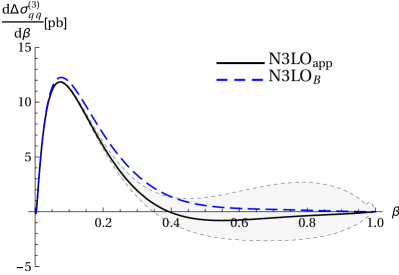
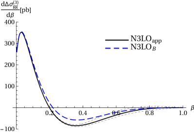
Figure 1: Partonic N³LO corrections to the cross section for $q\bar{q}\to t\bar{t}$ (left) and $gg\to t\bar{t}$ (right) at the LHC ($\sqrt{s}=13\,$TeV), multiplied with the parton luminosities. Black (solid): N³LO${}_{\text{app}}$ using (4.3), where the shaded gray area indicates the uncertainty estimated from varying the constants $C^{(3)}_{pp^{\prime}}$ and by using the kinematic variable $v$ instead of $\beta$. Blue (long-dashed): N³LO${}_{\text{B}}$ based on NNLL resummation.

From the comparison of the curves for our best prediction N³LO${}_{\text{app}}$ to the earliear approximation N³LO${}_{\text{B}}$ it can be seen that the effect of the corrections beyond NNLL is small in the limit $\beta\to 0$ but becomes significant for $\beta\gtrsim 0.3$. As already observed in [15], the corrections to the integrand $d\sigma/d\beta$ in the gluon-fusion channel become very large for $\beta\to 0$ and could lead to corrections of the order of several hundred picobarn to the total cross section at the LHC with $13$ TeV. In [15] it was speculated that this might indicate a poor convergence of the fixed-order expansion, despite an overall small numerical effect of resummation on the total cross section. In the total cross section, these large positive corrections are cancelled to a large extent by negative corrections for $\beta>0.2$, where, however, the threshold approximation is less reliable. The integrand approaches zero rapidly for $\beta\to 1$, which indicates that we are at least not including spuriously large corrections from the region where the threshold approximation breaks down. The gray band in the figures indicates the growing uncertainty of the threshold approximation for $\beta\gtrsim 0.4$. The relative uncertainty is larger in the quark-antiquark channel, however, the impact of both channels on the uncertainty of total cross section is similar as seen in (4.11) below.

4.2 Phenomenological results

In order to obtain predictions for the total hadronic top-quark pair production cross section, we use as default the MMHT2014NNLO PDFs [6, 93] with $\alpha_{s}(M_{Z})=0.118$. The top-quark pole mass value $m_{t}=173.3$ GeV is used. As central factorization and renormalization scales we choose $\mu_{r}=\mu_{f}=m_{t}.$ The contributions of the different partonic channels to the approximate N³LO corrections is obtained as

$$\Delta\sigma^{\mathrm{N}^{3}\mathrm{LO}_{\mathrm{app}}}_{q\bar{q}}(13\mathrm{TeV})= 1.86\mathrm{pb}$$

$$+(0.05\,C_{q\bar{q}}^{(3)}-3.91\,\delta c_{J,3}^{(1,0)}+3.06\,\delta c_{J,3}^{(2,0)}-0.30\,\gamma_{H,s}^{(2)})\times 10^{-3}\mathrm{pb},$$ (4.11a)

$$\Delta\sigma^{\mathrm{N}^{3}\mathrm{LO}_{\mathrm{app}}}_{gg}(13\mathrm{TeV})= 10.09\,\mathrm{pb}$$

$$+(0.12\,C_{gg}^{(3)}-7.38\,\delta c_{J,3}^{(1,0)}+6.15\,\delta c_{J,3}^{(2,0)}-0.56\,\gamma_{H,s}^{(2)})\times 10^{-3}\mathrm{pb},$$ (4.11b)

where we have indicated the contributions of the various unknown coefficients entering the scaling functions (4.3). As default we set the constant terms $C^{(3)}_{pp^{\prime}}$ to zero and estimate their size according to (4.6) and (4.9). Furthermore, we estimate kinematic ambiguities of the threshold approximation by using the expansion in terms of the variable $v$ instead of $\beta$. For the massive soft anomalous dimension and the potential coefficients we choose the default values and uncertainty estimates (4.4) and (4.5). We then obtain the prediction for the N³LO corrections to the cross section for $\mu_{f}=\mu_{r}=m_{t}$, and the uncertainties inherent in our approximations

$$\Delta\sigma^{\mathrm{N}^{3}\mathrm{LO}_{\mathrm{app}}}_{t\bar{t}}(13\mathrm{TeV})=12.25\underbrace{{}_{-6.24}^{+7.87}}_{C_{pp^{\prime}}^{(3)}}\underbrace{{}^{+5.3}_{-0.0}}_{\mathrm{kin.}}\pm\underbrace{0.11}_{\gamma_{H,s}^{(2)}}\pm\underbrace{0.60}_{\delta c_{J,3}^{(i,0)}}\mathrm{pb},$$ (4.12)

where “kin.” denotes the uncertainty due to the expansion in terms of $v$ instead of $\beta$. It is clearly seen that the uncertainties of the threshold expansion as estimated by the variation of the constants and the kinematic ambiguity dominate over the uncertainties due to the unknown soft anomalous dimension and potential coefficients.

In addition to the corrections included in the scaling functions (4.3), there is the distributional contribution arising from the third Coulomb correction (3.37). Inserting this correction to the potential function into the factorization formula (2.16) gives the correction

$$\Delta\sigma_{N_{1}N_{2}\to t\bar{t}X}^{C_{3}}=\sum_{p,p^{\prime}=q,\bar{q},g}\,L_{pp^{\prime}}(\frac{4m_{t}^{2}}{s},\mu_{f})\sum_{R=1,8}\frac{\alpha_{s}^{3}(\mu_{r})(-D_{R})^{3}m_{t}^{4}\zeta_{3}}{2s}H^{R}_{pp^{\prime},i}(m_{t},\mu_{r}).$$ (4.13)

The resulting correction at the LHC with $\sqrt{s}=13$ TeV is given by

$$\Delta\sigma_{t\bar{t}}^{C_{3}}(13\mathrm{TeV})=0.60\,\mathrm{pb},$$ (4.14)

in agreement with [38]. This contribution to the N³LO cross section is therefore of a similar size as the uncertainties due to the unknown coefficients in N³LL resummation.

Our default prediction is obtained by adding the correction $\Delta\sigma^{\mathrm{N}^{3}\mathrm{LO}_{\mathrm{app}}}_{t\bar{t}}$ from the threshold expansion of the scaling functions and the correction (4.13) to the NNLO cross section [9, 10, 11, 12],

$$\sigma^{\mathrm{N}^{3}\mathrm{LO}_{\mathrm{app}}}_{t\bar{t}}=\sigma^{\mathrm{NNLO}}_{t\bar{t}}+\Delta\sigma^{\mathrm{N}^{3}\mathrm{LO}_{\mathrm{app}}}_{t\bar{t}}+\Delta\sigma_{t\bar{t}}^{C_{3}}.$$ (4.15)

In order to estimate the scale uncertainty, we vary both renormalization and factorization scales independently in the interval $\frac{1}{2}\leq\mu_{f},\mu_{r}\leq 2$ with the constraint $\frac{1}{2}\leq\frac{\mu_{f}}{\mu_{r}}\leq 2$. We obtain

$$\sigma^{\mathrm{N}^{3}\mathrm{LO}_{\mathrm{app}}}_{t\bar{t}}(13\mathrm{TeV})=815.70^{+19.88(2.4\%)}_{-27.69(3.4\%)}(\mathrm{scale}){}^{+9.49(1.2\%)}_{-6.27(0.8\%)}(\mathrm{approx})\mathrm{pb},$$ (4.16)

where the “approx” uncertainty is obtained by adding the different contributions in (4.12) in quadrature. Compared to the NNLO result,

$$\sigma^{\mathrm{NNLO}}_{t\bar{t}}(13\mathrm{TeV})=802.85^{+28.12(3.5\%)}_{-44.97(5.6\%)}(\mathrm{scale})\mathrm{pb},$$ (4.17)

the approximate N³LO corrections increase the cross section moderately by $1.6\%$ and reduce the scale uncertainty to the $\pm 3\%$-level. Adding scale and approximation uncertainty in quadrature leads to a total perturbative uncertainty of ${}^{+2.7\%}_{-3.4\%}$, and therefore a reduction compared to the scale uncertainty of the NNLO result.

For other centre-of-mass energies at the LHC we obtain the results

$$\sigma^{\mathrm{N}^{3}\mathrm{LO}_{\mathrm{app}}}_{t\bar{t}}(7\mathrm{TeV}) =175.56^{+4.45(2.5\%)}_{-5.85(3.3\%)}(\mathrm{scale}){}^{+2.15(1.2\%)}_{-1.45(0.8\%)}(\mathrm{approx})\mathrm{pb},$$ (4.18)

$$\sigma^{\mathrm{N}^{3}\mathrm{LO}_{\mathrm{app}}}_{t\bar{t}}(8\mathrm{TeV}) =250.22_{-8.38(3.5\%)}^{+6.30(2.5\%)}(\mathrm{scale}){}^{+3.03(1.2\%)}_{-2.03(0.8\%)}(\mathrm{approx})\mathrm{pb},$$ (4.19)

$$\sigma^{\mathrm{N}^{3}\mathrm{LO}_{\mathrm{app}}}_{t\bar{t}}(14\mathrm{TeV}) =964.32_{-32.8(3.4\%)}^{+23.4(2.4\%)}(\mathrm{scale}){}^{+11.15(1.2\%)}_{-7.36(0.8\%)}(\mathrm{approx})\mathrm{pb}.$$ (4.20)

In addition to the uncertainty of the perturbative calculation estimated by the scale variation, the prediction of the hadronic cross section also relies on the value of the strong coupling constant and the PDFs, with their respective uncertainties. For the MMHT2014NNLO PDF, the combined PDF+$\alpha_{s}$ uncertainty of the NNLO top-quark pair-production cross section at the LHC is about $\pm 2.5\%$ [93], and therefore below the perturbative uncertainty of the approximate N³LO result (4.16). Following [94] we note that the evolution of the NNLO PDFs is performed including the three-loop splitting function, so the use of NNLO PDFs in an N³LO calculation is formally consistent, although the use of N³LO predictions in a PDF fit might lead to a non-negligible effect on the PDFs, in particular in the case of top-pair production [95]. In the following we discuss only the estimate of the perturbative uncertainties of our calculation.

It is interesting to compare the approximate N³LO result to the prediction of NNLL resummation matched to NNLO. Using the programs topixs 2.0.1 [18] and top++ 2.0 [17], which implement the combined soft-gluon and Coulomb resummation in momentum space [15] and soft-gluon resummation in Mellin space [16], respectively, we obtain

$$\sigma^{\mathrm{NNLL+NNLO}}_{t\bar{t}}(13\mathrm{TeV}) =807.13_{-36.83(4.6\%)}^{+15.63(1.9\%)}(\mathrm{scale}){}_{-12.9(1.8\%)}^{+19.15(2.5\%)}(\mathrm{approx.})\mathrm{pb} \mathrm{\texttt{(topixs)}},$$ (4.21)

$$\sigma^{\mathrm{NNLL+NNLO}}_{t\bar{t}}(13\mathrm{TeV}) =821.37^{+20.28(2.5\%)}_{-29.60(3.6\%)}(\mathrm{scale})\mathrm{pb} \mathrm{\texttt{(top++)}}.$$ (4.22)

The resummed Coulomb corrections beyond NNLO and bound-state corrections included in topixs only have a small effect, $+2.8$ pb for the bound-state corrections and less than one picobarn for higher-order Coulomb corrections. Furthermore, top++ includes the two-loop constants $C_{pp^{\prime}}^{(2)}$, which are part of the NNLL’ approximation. Setting these constants to zero, one obtains the top++ result of $812.20$ pb, which is closer to the result of topixs. The remaining difference indicates the size of sub-leading corrections, which are treated differently in the different resummation methods. The top++ result is also closer to the approximate N³LO prediction (4.16), which indicates the numerical relevance of the interplay of the two-loop constants and the soft threshold corrections. The total scale uncertainty of the two NNLL results is similar to each other and to that of the approximate N³LO correction. The topixs result also includes an estimate of the ambiguities of the resummation procedure, which includes the variation of the soft scale used in the momentum-space approach and the comparison of the expansion in $v$ and $\beta$. Since our approximate N³LO cross section is based on a partial N³LL resummation, the dependence on the soft-scale is reduced compared to the NNLL resummation and enters only in the estimate of the constant term. No attempt to estimate the ambiguities of the resummation procedure is made in top++. The fact that the approximate N³LO corrections are close to the resummed results indicates that the perturbative expansion is well-behaved, despite the large corrections to the partonic cross sections for small $\beta$ observed in Figure 1.

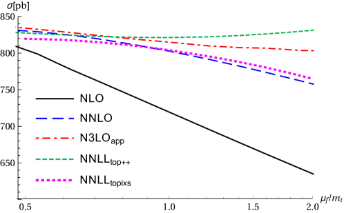
Figure 2: Scale-dependence ($\mu_{f}=\mu_{r}$) of the total cross section for the LHC with $\sqrt{s}=13$ TeV in various approximations.

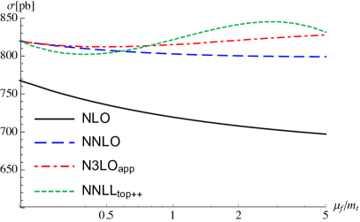
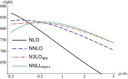
Figure 3: Total cross section for the LHC with $\sqrt{s}=13$ TeV in various approximations. Left: factorization-scale dependence (for $\mu_{r}=m_{t}$), right: renormalization-scale dependence (for $\mu_{f}=m_{t}$).

In Figure 2 we compare the factorization-scale dependence of the approximate N³LO cross section (red dash-dotted) to the NNLO result (blue, long-dashed) and the two resummed predictions from top++ (green, dashed) and topixs (magenta, dotted). The renormalization scale is set equal to the factorization scale. In the topixs calculation, all other scales are fixed to their default value. It is seen that the inclusion of the approximate N³LO corrections further flatten the scale dependence compared to the NNLO prediction and brings the curve closer to the resummed top++ result. In contrast, the topixs curve follows more closely the NNLO result. In Figure 3 we consider instead the factorization scale dependence for fixed renormalization scale and vice-versa. No results from topixs are shown since the renormalization scale is not separated from the factorization scale. Again it is seen that the inclusion of the approximate N³LO corrections stabilize the scale dependence and brings the result closer to the resummed prediction.

Approximate N³LO results were also published in [41, 42]. In these papers, no analytical results for the partonic cross sections are given so we can only compare numerical results for the total cross section. In addition, different PDFs are used for the results. The result of [41] is based on NNLL resummation for one-particle inclusive kinematics. At the LHC with $13$ TeV, a correction of $2.7\%$ relative to the NNLO result is found with a scale uncertainty of ${}^{+2.9\%}_{-2.0\%}$. The inherent uncertainty of the constructed approximation is not estimated. Ref. [42] constructs a partial N³LL soft resummation in Mellin space using similar input as our approximation, but without the contributions of the N³LO potential function. Furthermore, they also include $1/N$-suppressed contributions in Mellin space and information on the large-$\beta$ behaviour. As a result, they find larger corrections of $+4.2\%$ at $13$ TeV. The scale uncertainty of $\pm 2.7\%$ is comparable to that of our result (4.16). The scale-dependence of our result in Figure 3 is qualitatively similar to that shown in Figure 9 of [42]. An approximation corresponding to the standard Mellin-space resummation [16, 17] dubbed “$N$-soft” yields smaller corrections of $+2.3\%$ and is therefore closer to our prediction. The ambiguities of the approximation are estimated as $\pm 1.9\%$, which is larger than our estimate of ${}^{+1.2\%}_{-0.8\%}$ in (4.16). Therefore, while our default implementation results in a smaller correction than the one found in [41, 42], the results are consistent if the estimate of the uncertainties due to the threshold approximation are taken into account. In particular, using the expansion in terms of $v$ instead of $\beta$, we obtain a larger N³LO effect of $2.3\%$ which is in good agreement with the “$N$-soft” prediction of [42] and with [41]. It is interesting to compare our uncertainty estimate in more detail to the one of [42]. The “approx” uncertainty estimate in [42] includes contributions from two sources: the treatment of the subleading contributions in Mellin space and the parametric uncertainties due to the unknown three-loop constant term and the massive soft anomalous dimension for the colour-octet case. The estimate of the three-loop constant in Eqs. (5.3) and (5.5) of [42] amounts to an uncertainty of the cross section of $\pm 2.6$ pb at the LHC, which is smaller than our estimate in (4.12). In contrast, the estimate of the colour-octet soft-anomalous dimension in [42] amounts to an uncertainty of $\pm 4.6$ pb which is much more conservative than our estimate. Nevertheless, combining the two sources of parametric uncertainty in quadrature results in a similar parametric uncertainty as in our result. The dominant contribution to the uncertainty estimate of [42] arises from the ambiguities due to the treatment of the subleading contributions in Mellin space, which contribute an uncertainty of $\pm 1.8\%$, compared to our smaller estimate of the kinematic ambiguities using the expansion in $v$ instead of $\beta$. In addition, Ref. [42] estimates the uncertainty from omitting the N³LO approximation for the quark-antiquark and quark-gluon initial states as $1\%$. Instead, our result (4.11) includes the quark-antiquark channel with a contribution of only $0.2\%$.

5 Conclusions

We have constructed a combined resummation of threshold logarithms and Coulomb corrections to the total top-quark pair-production cross section at hadron colliders at partial N³LL accuracy and used the result to compute the threshold limit $\beta=\sqrt{1-\frac{4m_{t}^{2}}{\hat{s}}}\to 0$ of the partonic N³LO cross sections $q\bar{q}\to t\bar{t}$ and $gg\to t\bar{t}$. Our result makes use of the state-of-the-art N³LO results for the non-relativistic Green function from a calculation of $e^{-}e^{+}\to t\bar{t}$. We have also included contributions from sub-leading P-wave production channels and power-suppressed so-called next-to-eikonal corrections that give rise to threshold-enhanced N³LO corrections due to Coulomb enhancement. We have generalized the so-called $1/m^{2}$ one-loop potential in PNRQCD to the spin-singlet and colour-octet state. However, the three-loop massive soft-anomalous dimension, the two-loop $1/m$ potential in PNRQCD and the ultrasoft corrections to the non-relativistic Green function are currently not known for the production of top-quark pairs in a colour-octet state. We have estimated the uncertainty due to these missing ingredients on our result. The corrections from the N³LO Green function and the missing contributions for the colour-octet state affect the coefficients of the terms $\alpha_{s}^{3}\ln^{2,1}\beta$, and can have a larger numerical effect than the unknown three-loop massive soft-anomalous dimension.

Using the results for the threshold expansion of the partonic N³LO cross sections, we obtain moderate corrections $+1.5\%$ relative to the NNLO predictions for the LHC with $\sqrt{s}=13$ TeV and a reduction of the factorization- and renormalization-scale uncertainty to the $\pm 3\%$-level. We estimate the uncertainty of our prediction due to the threshold approximation to be about $\pm 1\%$. The total perturbative uncertainty therefore approaches a similar level as the PDF+$\alpha_{s}$ uncertainty of $\pm 2.5\%$. Our default prediction is smaller than other approximate N³LO predictions [41, 42] but consistent with these results if the estimate of the uncertainties due to the threshold approximation are taken into account. The difference between these predictions indicates the possible size of subleading terms in the threshold expansion.

We have explicitly provided all necessary ingredients to implement our results in a numerical program. Since the numerical result of the approximate N³LO corrections and their scale uncertainty are close to the resummed NNLL predictions, this provides a simple, computationally less expensive way to obtain the leading corrections beyond NNLO. We plan to include these results in a future version of topixs, as well the implementation of the fully resummed threshold corrections at partial N³LL accuracy.

Acknowledgments

We would like to thank Martin Beneke for useful discussions and for making a copy of Ref. [80] available. The work of CS is supported by the Heisenberg Programme of the DFG. We acknowledge support by the Munich Institute for Astro- and Particle Physics (MIAPP) of the DFG cluster of excellence “Origin and Structure of the Universe” during parts of this work.

Note added

In this version v3 of the arXiv submission of the paper, typos in the coefficients of the $\ln\beta$-terms in the scaling functions $f^{(3,0)}_{gg(1)}$ in (4.3), $f^{(3,1)}_{gg(8)}$ in (C.12), and the $1/\beta$-term in $f^{(3,2)}_{gg(1)}$ in (C.7) have been corrected. These typos do not affect the implementation used to compute the numerical results of the cross sections. However, in addition the scale dependence in the results (4.16) and (4.18)–(4.20) has been corrected.

In the latest version 3.0 of the program topixs, which can be obtained from

http://users.ph.tum.de/t31software/topixs/

the approximate N³LO corrections computed in this paper are available as an option by setting APPROX_NNNLO=1 in the input file topixs.cfg.

Appendix A Renormalization group functions

In this appendix we give explicit results for the NNLO expansion of the hard and soft functions. The various anomalous dimensions appearing in the expressions are expanded in the strong coupling constant according to

$$\gamma=\sum_{n}\gamma^{(n)}\left(\frac{\alpha}{4\pi}\right)^{n+1}.$$ (A.1)

For the expansion of the $\beta$-function and the splitting functions we use the conventions

$$\beta(\alpha_{s}) =-\alpha_{s}\sum_{n=0}^{\infty}\beta_{n}\left(\frac{\alpha_{s}}{4\pi}\right)^{n+1}$$ (A.2)

$$P_{p/p^{\prime}}(x) =\sum_{n=0}^{\infty}P_{p/p^{\prime}}^{(n)}(x)\left(\frac{\alpha_{s}}{4\pi}\right)^{n+1}$$ (A.3)

which corresponds to $\beta_{0}=\frac{11}{3}C_{A}-\frac{4}{3}n_{l}T_{f}$.

A.1 Two-loop hard functions

The perturbative expansion of the hard function in the QCD coupling can be written as

$$H^{R}_{pp^{\prime}}(\mu_{h})=H^{R(0)}_{pp^{\prime}}(\mu_{h})\left[1+\sum_{n}\left(\frac{\alpha_{s}(\mu_{h})}{4\pi}\right)^{n}h^{R(n)}_{pp^{\prime}}(\mu_{h})\right]\,,$$ (A.4)

where we have extracted the leading-order hard function $H^{R(0)}_{pp^{\prime}}(\mu_{h})$ that includes a factor $\alpha_{s}^{2}(\mu_{h})$. We also left the spin dependence implicit. The relation of the one- and two-loop coefficients at a scale $\mu$ to the initial conditions at $\mu_{h}=m_{t}$ follow from the evolution equation (3.1):

$$h^{R(1)}_{pp^{\prime}}(\mu) =-C_{rr^{\prime}}\gamma^{(0)}_{\text{cusp}}\ln^{2}\left(\frac{m_{t}}{\mu}\right)-2(\gamma^{V(0)}_{i}+2\beta_{0}+C_{rr^{\prime}}\gamma^{(0)}_{\text{cusp}}\ln 2)\ln\left(\frac{m_{t}}{\mu}\right)+h^{R(1)}_{pp^{\prime}}(m_{t}),$$ (A.5)

$$h^{R(2)}_{pp^{\prime}}(\mu) =\frac{1}{2}C_{rr^{\prime}}^{2}(\gamma^{(0)}_{\text{cusp}})^{2}\ln^{4}\left(\frac{m_{t}}{\mu}\right)+2C_{rr^{\prime}}\gamma^{(0)}_{\text{cusp}}\left(\gamma^{V(0)}_{i}+C_{rr^{\prime}}\gamma^{(0)}_{\text{cusp}}\ln 2+\frac{7}{3}\beta_{0}\right)\ln^{3}\left(\frac{m_{t}}{\mu}\right)$$

$$\quad+\Bigl{[}\left(\gamma^{V(0)}_{i}+2\beta_{0}\right)\left(2\gamma^{V(0)}_{i}+6\beta_{0}+5C_{rr^{\prime}}\gamma^{(0)}_{\text{cusp}}\ln 2\right)$$

$$\quad-C_{rr^{\prime}}\left(\gamma^{(1)}_{\text{cusp}}+\gamma^{(0)}_{\text{cusp}}h^{R(1)}_{pp^{\prime}}(m_{t})-2C_{rr^{\prime}}(\gamma^{(0)}_{\text{cusp}})^{2}\ln^{2}2+\gamma^{V(0)}_{i}\gamma^{(0)}_{\text{cusp}}\ln 2\right)\Bigr{]}\ln^{2}\left(\frac{m_{t}}{\mu}\right)$$

$$\quad-\Bigl{[}2\gamma^{V(1)}_{i}+\gamma_{J}^{R,S(1)}+2C_{rr^{\prime}}\gamma^{(1)}_{\text{cusp}}\ln 2+4\beta_{1}$$

$$\quad+2\left(\gamma^{V(0)}_{i}+3\beta_{0}+C_{rr^{\prime}}\gamma^{(0)}_{\text{cusp}}\ln 2\right)h^{R(1)}_{pp^{\prime}}(m_{t})\Bigr{]}\ln\left(\frac{m_{t}}{\mu}\right)+h^{R(2)}_{pp^{\prime}}(m_{t}).$$ (A.6)

Here the factor $\alpha_{s}^{2}(\mu_{h})$ in the leading-order hard function was taken into account. We have also defined the colour factor $C_{rr^{\prime}}=C_{r}+C_{r^{\prime}}$.

Expanding the resummation formula for the NNLL and NNLL’ approximations to $\mathcal{O}(\alpha_{s})$ and $\mathcal{O}(\alpha_{s}^{2})$, respectively, one obtains the relation between the constant terms $C_{pp}^{R(n)}$ in the threshold expansion of the NLO and NNLO cross sections to the coefficients of the hard functions at the scale $\mu_{h}=m_{t}$:

$$h^{R(1)}_{pp^{\prime}}(m_{t}) =C_{pp}^{R(1)}-C_{rr^{\prime}}\left(32+36\ln^{2}2-48\ln 2-\frac{11\pi^{2}}{6}\right)-12C_{R}(1-\ln 2),$$ (A.7)

$$h^{R(2)}_{pp^{\prime}}(m_{t}) =C_{pp}^{R(2)}-\tilde{s}_{i}^{R(2)}(0)-(4\pi)^{2}(c_{J,2}+\gamma_{J}^{R,S(1)}\ln 2)-\frac{4\pi^{4}D_{R}^{2}}{3}\left[d_{J}-\frac{3}{8}\right]$$

$$\quad-h^{R(1)}_{pp^{\prime}}(m_{t})\Biggl{[}C_{rr^{\prime}}\left(4(8+9\ln^{2}2)-48\ln 2-\frac{11\pi^{2}}{6}\right)+12C_{R}(1-\ln 2)\Biggr{]}$$

$$\quad-C_{rr^{\prime}}^{2}\Biggl{[}24\left(27\ln^{4}2-72\ln^{3}2+144\ln^{2}2-192\ln 2+128\right)$$

$$\quad-\frac{70\pi^{2}}{3}\left(9\ln^{2}2-12\ln 2+8\right)-\frac{7\pi^{4}}{3}+448(3\ln 2-2)\zeta_{3}\Biggr{]}$$

$$\quad-C_{rr^{\prime}}C_{R}\left[-16\left(27\ln^{3}2-63\ln^{2}2+84\ln 2-56\right)-\frac{\pi^{2}}{3}(164-210\ln 2)-224\zeta_{3}\right]$$

$$\quad-C_{rr^{\prime}}C_{A}\Bigl{[}268\ln^{2}2-\frac{4024\ln 2}{9}+\frac{8048}{27}+\frac{2\pi^{4}}{3}$$

$$\quad-\frac{1}{3}\pi^{2}\left(36\ln^{2}2-59\ln 2+84\right)+28(3\ln 2-2)\zeta_{3}\Bigr{]}$$

$$\quad-C_{rr^{\prime}}n_{f}T_{F}\left[\frac{8}{27}\left(-270\ln^{2}2+444\ln 2-296\right)+\frac{4\pi^{2}}{9}(12-3\ln 2)\right]$$

$$\quad-C_{R}^{2}\left[24\left(3\ln^{2}2-6\ln 2+4\right)-4\pi^{2}\right]$$

$$\quad-C_{R}\Bigl{[}C_{A}\left(\frac{196}{9}-\frac{4}{3}\pi^{2}+8\zeta_{3}\right)(2-3\ln 2)-n_{f}T_{F}\frac{1}{9}\left(160-240\ln 2\right)\Bigr{]}$$

$$\quad-\beta_{0}\Biggl{[}C_{rr^{\prime}}\left(-24(3\ln^{2}2-6\ln 2+8)\ln 2+11\pi^{2}\ln 2-\frac{112\zeta_{3}}{3}-\frac{22\pi^{2}}{3}+128\right)$$

$$\quad+12C_{R}\left(3\ln^{2}2-6\ln 2+4-\frac{\pi^{2}}{6}\right)\Biggr{]}.$$ (A.8)

Although the natural hard scale is of the order $2m_{t}$, these relations simplify for the choice $\mu_{h}=m_{t}$ made here. In particular, they become independent of the anomalous dimensions $\gamma^{V}_{i}$, which do not obey Casimir scaling. In the NNLO coefficient, the constant terms in the two-loop soft function (3.18) and the NNLO potential function (3.35) enter. Additionally, the coefficient $d_{J}$ from kinematic corrections to the matching of the potential function (3.19) and the relation (3.20) of the variables $v$ and $\beta$ have been taken into account. The constants $C_{pp^{\prime}}^{R(2)}$ in (A.8) are related to the results in the conventions of [34], here denoted by a bar, according to

$$C_{pp^{\prime}}^{R(2)}=\bar{C}_{pp^{\prime}}^{R(2)}+\frac{4\pi^{4}D_{R}^{2}}{3}-4\pi^{2}D_{R}^{2}\left(1+\frac{\pi^{2}}{3}\right)h^{(0),R}_{pp^{\prime},P}.$$ (A.9)

Here the first correction term arises from multiplying the prefactor $4m_{t}^{2}/\hat{s}=1-\beta^{2}$ with the second Coulomb correction. Further, since no spin decomposition is performed in the results for the constants $\bar{C}_{pp}^{R(2)}$ in [34], the P-wave contribution (3.48) with the coefficient (3.45) was subtracted to obtain the hard function for the S-wave process.

For the number of light flavours $n_{f}=5$ and using $N_{C}=3$ and $T_{F}=1/2$, but keeping the colour representations arbitrary, the NNLO result becomes

$$h^{R(2)}_{pp^{\prime}}(m_{t}) =\bar{C}_{pp^{\prime}}^{R(2)}-\tilde{s}_{i}^{R(2)}(0)+h^{R(1)}_{pp^{\prime}}(m_{t})(2.06903C_{rr^{\prime}}-3.68223C_{R})$$

$$\quad-5.41462C_{rr^{\prime}}^{2}+25.0828C_{rr^{\prime}}C_{R}+35.5195C_{rr^{\prime}}+8.69899C_{R}^{2}+35.9266C_{R}$$

$$\quad+D_{R}^{2}(-554.062+61.0012\,\nu_{\mathrm{spin}}^{S}-78.9568\,\nu_{\mathrm{spin}}^{S,\epsilon}-129.879\,d_{J}-169.357h^{(0),R}_{pp^{\prime},P})$$

$$\quad+D_{R}(263.804+15.2503{\nu_{\mathrm{ann}}^{R,S}}^{(0)}).$$ (A.10)

A.2 Two-loop soft function

We consider the perturbative expansion of the soft function in Laplace space,

$$\tilde{s}_{i}^{R}(\rho,\mu)=\sum_{n=0}^{\infty}\left(\frac{\alpha_{s}(\mu)}{4\pi}\right)^{n}\tilde{s}_{i}^{(n)R}(\rho,\mu).$$ (A.11)

The coefficients of the variable $\rho$ are fixed by the anomalous dimensions in the evolution equation (3.14), so the only required input are constant coefficients $\tilde{s}_{i}^{(n)R}(0)$:

$$\tilde{s}_{i}^{(0)R}(\rho,\mu) =1,$$ (A.12)

$$\tilde{s}_{i}^{(1)R}(\rho,\mu) =\frac{C_{rr^{\prime}}\gamma_{\text{cusp}}^{(0)}}{4}\,\rho^{2}+C_{R}\gamma_{H,s}^{(0)}\,\rho+\tilde{s}_{i}^{(1)R}(0),$$ (A.13)

$$\tilde{s}_{i}^{(2)R}(\rho,\mu) =\frac{1}{2}\left(\frac{C_{rr^{\prime}}\gamma_{\text{cusp}}^{(0)}}{4}\right)^{2}\,\rho^{4}+\frac{C_{rr^{\prime}}\gamma_{\text{cusp}}^{(0)}}{12}(3C_{R}\gamma_{H,s}^{(0)}-\beta_{0})\,\rho^{3}$$

$$\quad+\frac{1}{4}\left[C_{rr^{\prime}}(\gamma_{\text{cusp}}^{(1)}+\gamma_{\text{cusp}}^{(0)}\tilde{s}_{i}^{(1)R}(0))+2C_{R}\gamma_{H,s}^{(0)}(C_{R}\gamma_{H,s}^{(0)}-\beta_{0})\right]\rho^{2}$$

$$\quad+\left[C_{rr^{\prime}}\gamma_{s}^{(1)}+C_{R}\gamma_{H,s}^{(1)}+\tilde{s}_{i}^{(1)R}(0)(C_{R}\gamma_{H,s}^{(0)}-\beta_{0})\right]\rho+\tilde{s}_{i}^{(2)R}(0).$$ (A.14)

Here it was used that the soft anomalous dimensions of the light partons $\gamma_{s}$ vanish at the one-loop level. The initial conditions $\tilde{s}_{i}^{(2)R}(0)$ given in (3.18) were obtained from two-loop calculations of the soft function in the literature by noting that the soft function in Laplace space is obtained from the position-space result in [32] by the simple replacement $L=2\ln\left(\frac{iz_{0}\mu e^{\gamma_{E}}}{2}\right)\to-\rho$ and from the Mellin-space result in [33] by the replacement $L=\ln\left(\frac{\mu N}{m_{t}}\right)\to-2\rho$.

The explicit results for the cusp anomalous dimension are given by

$$\gamma^{(0)}_{\text{cusp}} =4,$$

$$\gamma^{(1)}_{\text{cusp}} =\left(\frac{268}{9}-\frac{4\pi^{2}}{3}\right)C_{A}-\frac{80}{9}T_{F}n_{f},$$

$$\gamma^{(2)}_{\text{cusp}} =C_{A}^{2}\left(\frac{490}{3}-\frac{536\pi^{2}}{27}+\frac{44\pi^{4}}{45}+\frac{88}{3}\zeta_{3}\right)+C_{A}T_{F}n_{f}\left(-\frac{1672}{27}+\frac{160\pi^{2}}{27}-\frac{224}{3}\zeta_{3}\right)$$

$$\qquad+C_{F}T_{F}n_{f}\left(-\frac{220}{3}+64\zeta_{3}\right)-\frac{64}{27}T_{F}^{2}n_{f}^{2}.$$ (A.15)

The one- and two-loop coefficients of the soft anomalous dimensions of the light partons are given in [32] while the three-loop coefficient can be obtained from the results for $\gamma^{(2)p}$ and $\gamma^{(2)\phi,p}$ in  [72, 32, 45]

$$\gamma_{s}^{(0)} =0,$$

$$\gamma_{s}^{(1)} =C_{A}\left(-\frac{404}{27}+\frac{11\pi^{2}}{18}+14\zeta_{3}\right)+T_{F}n_{f}\left(\frac{112}{27}-\frac{2\pi^{2}}{9}\right),$$

$$\gamma_{s}^{(2)} =C_{A}^{2}\left(-\frac{136781}{1458}+\frac{6325\pi^{2}}{486}-\frac{44\pi^{4}}{45}+\frac{658}{3}\zeta_{3}-\frac{44\pi^{2}}{9}\zeta_{3}-96\zeta_{5}\right)$$

$$+C_{A}T_{F}n_{f}\left(\frac{11842}{729}-\frac{1414\pi^{2}}{243}+\frac{8\pi^{4}}{15}-\frac{728}{27}\zeta_{3}\right)$$

$$+C_{F}T_{F}n_{f}\left(\frac{1711}{27}-\frac{2\pi^{2}}{3}-\frac{8\pi^{4}}{45}-\frac{304}{9}\zeta_{3}\right)$$

$$+T_{F}^{2}n_{f}^{2}\left(\frac{4160}{729}+\frac{40\pi^{2}}{81}-\frac{224}{27}\zeta_{3}\right).$$ (A.16)

The heavy particle anomalous-dimension coefficients are only known up to two loops

$$\gamma_{H,s}^{(0)} =-2,$$ (A.17)

$$\gamma_{H,s}^{(1)} =-C_{A}\left(\frac{98}{9}-\frac{2\pi^{2}}{3}+4\zeta_{3}\right)+\frac{40}{9}T_{F}n_{f}.$$

Appendix B Potential corrections

B.1 Potential for general spin and colour states

In this appendix we provide the projection of the PNRQCD potential onto spin-singlet and triplet states and obtain the one-loop $1/m^{2}$ potential for the colour-octet case. The conventions of the PNRQCD Lagrangian follow [35]. The general colour dependence of the quark-antiquark potential can be decomposed in the two equivalent forms

$$V_{ab;cd}({\bf p},{\bf p}^{\prime}) =V_{S}({\bf p},{\bf p}^{\prime})\delta_{ab}\delta_{cd}+V_{T}({\bf p},{\bf p}^{\prime})T^{A}_{ab}T^{A}_{cd}$$ (B.1)

$$=V^{1}({\bf p},{\bf p}^{\prime})\frac{1}{N_{c}}\delta_{cb}\delta_{ad}+V^{8}({\bf p},{\bf p}^{\prime})2T^{A}_{cb}T^{A}_{ad},$$

where the potential coefficients in the two conventions are related by

$$V^{R}=V_{S}-D_{R}V_{T},$$ (B.2)

with the colour factor (3.25). The potential for arbitrary spin in a given colour channel $R$ is of the form [35]

$$V^{R}({\bf p},{\bf p}^{\prime}) = {\cal V}^{R}_{C}(\alpha_{s})\frac{4\pi D_{R}\alpha_{s}}{{\bf q}^{2}}-{\cal V}^{R}_{1/m}(\alpha_{s})\frac{\pi^{2}(4\pi)D_{R}\alpha_{s}}{m_{t}|{\bf q}|}$$ (B.3)

$$-\,{\cal V}^{R}_{\delta}(\alpha_{s})\frac{2\pi D_{R}\alpha_{s}}{m_{t}^{2}}+{\cal V}_{s}^{R}(\alpha_{s})\frac{\pi D_{R}\alpha_{s}}{4m_{t}^{2}}[\sigma_{i},\sigma_{j}]\otimes[\sigma_{i},\sigma_{j}]$$

$$+\,{\cal V}^{R}_{p}(\alpha_{s})\frac{2\pi D_{R}\alpha_{s}({\bf p}^{2}+{\bf p}^{\prime 2})}{m_{t}^{2}{\bf{q}}^{2}}-{\cal V}^{R}_{hf}(\alpha_{s})\frac{\pi D_{R}\alpha_{s}}{4m_{t}^{2}{\bf q}^{2}}[\sigma_{i},\sigma_{j}]q_{j}\otimes[\sigma_{i},\sigma_{k}]q_{k}$$

$$+{\cal V}^{R}_{so}(\alpha_{s})\frac{3\pi D_{R}\alpha_{s}}{2m_{t}^{2}{\bf q}^{2}}\Bigg{(}[\sigma_{i},\sigma_{j}]q_{i}p_{j}\otimes 1-1\otimes[\sigma_{i},\sigma_{j}]q_{i}p_{j}\Bigg{)}+\ldots\,.$$

Here the spin-dependence is written in a tensor-product notation, $a\otimes b$, where $a$ ($b$) refers to the spin-matrix on the quark (antiquark). In addition to (B.3), also the so-called annihilation contribution from local NRQCD four-fermion operators must be included for hadronic top-quark production. This is discussed in App. B.2. The potential (B.3) can be further decomposed into spin-singlet and triplet contributions according to

$$V^{R}({\bf p},{\bf p}^{\prime})=\frac{1}{2}V^{R,0}({\bf p},{\bf p}^{\prime})\,1\otimes 1+\frac{1}{2}V^{R,1}({\bf p},{\bf p}^{\prime})\,\sigma_{i}\otimes\sigma_{i},$$ (B.4)

where the spin projection in $d-1$ space dimensions can be performed as discussed in Section 4.5 of [35]. In this way, one obtains the colour- and spin-projected potential

$$V^{R,S}({\bf p},{\bf p}^{\prime}) = \frac{4\pi\alpha_{s}D_{R}}{{\bf q}^{2}}\bigg{[}\,{\cal V}^{R}_{C}-{\cal V}^{R}_{1/m}\,\frac{\pi^{2}\,|\bf{q}|}{m_{t}}+{\cal V}^{R,S}_{1/m^{2}}\,\frac{{\bf q}^{2}}{m_{t}^{2}}+{\cal V}_{p}^{R}\,\frac{{\bf p}^{2}+{\bf p}^{\prime\,2}}{2m_{t}^{2}}\,\bigg{]}.$$ (B.5)

Additionally, the term $\partial^{4}/8m_{t}^{3}$ in the PNRQCD Lagrangian is also treated as a potential (cf. Eq.(4.60) of [35]).

We require the Coulomb-potential up to two-loop accuracy, which reads in four dimensions

$${\cal V}_{C}^{R}=1+\frac{\alpha_{s}}{4\pi}\left(a_{1}+\beta_{0}\ln\frac{\mu^{2}}{{\bf q}^{2}}\right)+\left(\frac{\alpha_{s}}{4\pi}\right)^{2}\left(a_{2}^{R}+(2a_{1}\beta_{0}+\beta_{1})\ln\frac{\mu^{2}}{{\bf q}^{2}}+\beta_{0}^{2}\ln^{2}\frac{\mu^{2}}{{\bf q}^{2}}\right)+\dots$$ (B.6)

with the one-loop coefficient

$$a_{1}=\frac{31}{9}C_{A}-\frac{20}{9}n_{l}T_{f}.$$ (B.7)

The two-loop coefficient depends on the colour representation [78, 79],

$$a_{2}^{1} =C_{A}^{2}\left(\frac{4343}{162}+4\pi^{2}-\frac{\pi^{4}}{4}+\frac{22}{3}\zeta_{3}\right)-C_{A}T_{F}n_{f}\left(\frac{1798}{81}+\frac{56}{3}\zeta_{3}\right)$$ (B.8)

$$-C_{F}T_{F}n_{f}\left(\frac{55}{3}-16\zeta_{3}\right)+(T_{F}n_{f})^{2}\frac{400}{81},$$

$$a_{2}^{8} =a_{2}^{1}+C_{A}^{2}(\pi^{4}-12\pi^{2}).$$

The $1/m$ potential for the colour-singlet case is quoted in Section 4.4.2 of [35]. The colour-octet one-loop result can be found in [55], while the corresponding two-loop result is currently not known. The resulting uncertainty on our predictions is estimated as discussed in Section 4.1.

The spin-dependence in (B.5) enters only through the $1/m^{2}$ potential

$${\cal V}^{R,S}_{1/m^{2}}=-\frac{1}{2}{\cal V}^{R}_{\delta}+\left(v^{S}(\epsilon)+\frac{1}{2}\right)\left[{\cal V}^{R}_{hf}-(d-1){\cal V}^{R}_{s}\right],$$ (B.9)

where in $d=4-2\epsilon$ dimensions

$$v^{S}(\epsilon)=\begin{cases}-\frac{1}{2}\epsilon,&S=0\\ \frac{2\epsilon^{2}+\epsilon-4}{6-4\epsilon},&S=1\end{cases}$$ (B.10)

At tree level, the potential coefficients in the $1/m^{2}$ potential are

$${\cal V}_{\delta}^{R(0)} =1, {\cal V}_{hf}^{R(0)} =1, {\cal V}_{s}^{R(0)} =0, {\cal V}_{p}^{R(0)} =1,$$ (B.11)

so that

$${\cal V}^{R,S,(0)}_{1/m^{2}}=v^{S}(\epsilon).$$ (B.12)

The one-loop result for the colour-singlet $1/m^{2}$ potential is given in Section 4.4.3 of [35]. We argue now that the colour-octet result can be obtained from the singlet case after an appropriate adjustment of the colour factors. Following [35], the one-loop $1/m^{2}$ potential can be calculated from an NRQCD computation consisting of a “hard” contribution of tree diagrams with one-loop matching coefficients, and a “soft” contribution of one-loop NRQCD diagrams. The soft contributions receive contributions from the diagrams in Fig. 9 of [35]. It can be seen from the NRQCD Feynman rules that the colour factors are either the same as the box or crossed-box topologies in the full QCD diagrams,

$$C^{\text{box}}_{ab;cd} =(T^{A}T^{B})_{ab}(T^{B}T^{A})_{cd}\,, C^{\text{c-box}}_{ab;cd} =(T^{A}T^{B})_{ab}(T^{A}T^{B})_{cd},$$ (B.13)

or can be written as linear combinations thereof. The projection of these colour factors on the singlet and octet states can be written in the form $C^{\text{box}}\to D_{R}^{2}$ and $C^{\text{c-box}}\to D_{R}\left(D_{R}+\frac{C_{A}}{2}\right)$ so that in both cases the result for the general representation is obtained from the singlet result by the replacement $(-C_{F})\to D_{R}$. There are further contributions from the abelian vertex correction, self-energy insertions and charge-renormalization counterterms. These contributions contain explicit factors of $C_{F}$ but are scaleless, so they do not contribute to the finite part of the potential. The hard corrections receive contributions from one-loop matching coefficients of four-fermion operators, the NRQCD quark-gluon vertex and the gluon two-point functions. Since the former arise from box-diagrams in full QCD, the same replacement of colour factors as in the soft contribution can be applied, while the colour factors arising from the coefficients $d_{i}$ of the vertex and two-point functions are unmodified. As result, we obtain the $1/m^{2}$ potential for the spin-singlet/triplet and colour-singlet/octet states

$${\cal V}_{1/m^{2}}^{R,S,(1)} = \Bigg{[}\bigg{(}\frac{\mu^{2}}{\bf{q}^{2}}\bigg{)}^{\!\epsilon}-1\Bigg{]}\,\frac{1}{\epsilon}\,\bigg{(}\,-\frac{7}{3}D_{R}-\frac{25+21v^{S}(\epsilon)}{6}C_{A}\,+\beta_{0}\,v^{S}(\epsilon)\bigg{)}$$ (B.14)

$$+\,\Bigg{[}\left(\frac{{\mu}^{2}}{m_{t}^{2}}\right)^{\!\epsilon}-1\Bigg{]}\,\frac{1}{\epsilon}\,\bigg{(}\,\frac{4C_{F}+3D_{R}}{3}+\frac{17+21v^{S}(\epsilon)}{6}C_{A}\,\bigg{)}$$

$$+\bigg{(}\frac{\mu^{2}}{\bf{q}^{2}}\bigg{)}^{\!\epsilon}\,v^{S(1)}_{q}(\epsilon)+\bigg{(}\frac{{\mu}^{2}}{m_{t}^{2}}\bigg{)}^{\!\epsilon}\,v^{S(1)}_{m}(\epsilon),\quad$$

with

$$v^{S,(1)}_{q}(\epsilon) =\frac{D_{R}}{3}-\frac{7}{4}C_{A}-\left(\frac{5}{9}C_{A}+\frac{20}{9}\,T_{F}n_{f}\right)v^{S}(\epsilon)+O(\epsilon),$$

$$v^{S,(1)}_{m}(\epsilon) =\frac{11\,D_{R}}{3}+2C_{F}-\frac{C_{A}}{4}+(6D_{R}+4C_{F}+3C_{A})v^{S}(\epsilon)+\frac{4}{15}\,T_{F}+\,O(\epsilon),$$ (B.15)

where the $O(\epsilon)$ contributions do not contribute to the logarithmic corrections considered here. This result agrees with an explicit calculation of the singlet and octet cases [80]. The potential coefficient ${\cal V}_{p}^{R,(1)}$ is the same for both the singlet and the octet case.

B.2 Annihilation contribution

The contribution of local four-fermion operators to the NRQCD Lagrangian is given by

$$\delta\mathcal{L}_{4f}=-\delta V_{ab;cd}^{4f}\;\left(\psi_{c}^{\dagger}\chi_{b}\chi^{\dagger}_{a}\psi_{d}\right),$$ (B.16)

where the labels collectively denote the spin and colour quantum numbers. This convention agrees with [55]. The four-fermion Lagrangian can be decomposed into contributions with definite spin and colour quantum numbers, analogously to (B.1) and (B.4)

$$-\delta\mathcal{L}_{4f} =\frac{\delta V_{4f}^{1,0}}{2N_{C}}\left(\psi^{\dagger}\chi\right)\left(\chi^{\dagger}\psi\right)+\delta V_{4f}^{8,0}\;\left(\psi^{\dagger}T^{A}\chi\right)\left(\chi^{\dagger}T^{A}\psi\right)$$ (B.17)

$$\quad+\frac{\delta V_{4f}^{1,1}}{2N_{C}}\left(\psi^{\dagger}\sigma^{i}\chi\right)\left(\chi^{\dagger}\sigma^{i}\psi\right)+\delta V_{4f}^{8,1}\;\left(\psi^{\dagger}T^{A}\sigma^{i}\chi\right)\left(\chi^{\dagger}T^{A}\sigma^{i}\psi\right).$$

The relation to the coefficients $d^{c}$ introduced in [81] is given by

$$\delta V_{4f}^{1,0} =-2N_{C}\frac{d^{c}_{ss}}{m_{t}^{2}}, \delta V_{4f}^{8,0} =-\frac{d^{c}_{vs}}{m_{t}^{2}}, \delta V_{4f}^{1,1} =-2N_{C}\frac{d^{c}_{sv}}{m_{t}^{2}}, \delta V_{4f}^{8,1} =-\frac{d^{c}_{vv}}{m_{t}^{2}}.$$ (B.18)

The contributions to the four-fermion operators arising from “scattering” diagrams (i.e. diagrams present if $\psi$ and $\chi$ correspond to different quark flavours) are already included in the PNRQCD $1/m^{2}$ potential discussed in appendix B.1. For the “annihilation” contributions (i.e. diagrams only present for identical quark flavours) we use the notation

$$\delta V_{\mathrm{ann}}^{R,S}=\frac{\pi\alpha_{s}}{m_{t}^{2}}\nu_{\mathrm{ann}}^{R,S}.$$ (B.19)

The perturbative corrections to the annihilation coefficients up to NLO will be written in the form

$$\nu_{\mathrm{ann}}^{R,S}(\mu)={\nu_{\mathrm{ann}}^{R,S}}^{(0)}+\frac{\alpha_{s}}{4\pi}{\nu_{\mathrm{ann}}^{R,S}}^{(1)}(\mu)+\mathcal{O}(\alpha_{s}^{2}).$$ (B.20)

The scale-dependence of the NLO coefficient only enters through the running of $\alpha_{s}$:

$${\nu_{\mathrm{ann}}^{R,S}}^{(1)}(\mu)={\nu_{\mathrm{ann}}^{R,S}}^{(1)}(2m_{t})-2\beta_{0}\ln\left(\frac{2m_{t}}{\mu}\right){\nu_{\mathrm{ann}}^{R,S}}^{(0)}.$$ (B.21)

At LO, the only non-vanishing correction is

$${\nu_{\mathrm{ann}}^{8,1}}^{(0)}=1,$$ (B.22)

which is relevant for the quark-antiquark channel. At NLO there are also non-vanishing annihilation contributions in the spin-singlet channel, which are relevant for gluon-induced top production [81]:

$${\nu_{\mathrm{ann}}^{8,1}}^{(1)}(2m_{t}) =-\frac{20}{9}T_{F}n_{l}-\frac{32}{9}T_{F}-16C_{F}+C_{A}\left(\frac{109}{9}+\frac{22}{3}\ln 2\right),$$ (B.23)

$${\nu_{\mathrm{ann}}^{1,0}}^{(1)}(2m_{t}) =-8C_{F}(1-\ln 2),$$

$${\nu_{\mathrm{ann}}^{8,0}}^{(1)}(2m_{t}) =-4C_{F}\left(-\frac{3C_{A}}{2}+4C_{F}\right)(1-\ln 2).$$

Here we have neglected imaginary parts, which contribute to toponium decay into light hadrons and should not be taken into account for the total cross section for $pp\to t\bar{t}\to b\bar{b}W^{+}W^{-}$.

The corrections to the NNLO Green function due to an insertion of an annihilation correction is [55]

$$\delta_{\mathrm{ann}}G_{R}^{(1)S}=-\frac{\pi\alpha_{s}}{m_{t}^{2}}{\nu_{\mathrm{ann}}^{R,S}}^{(0)}\left[G_{R}^{(0)}(0,0;E)\right]^{2},$$ (B.24)

with the resulting correction to the potential function at $\mathcal{O}(\alpha_{s}^{2})$

$$\Delta_{\mathrm{ann}}J_{R}^{S(2)}(E)=J^{(0)}(E)\alpha_{s}^{2}(\mu)\frac{D_{R}}{4}{\nu_{\mathrm{ann}}^{R,S}}^{(0)}(2L_{E}+1).$$ (B.25)

The annihilation corrections to the N³LO Green function are obtained from the master formula in [35] as

$$\delta_{\mathrm{ann}}G_{R}^{(2)S}=-\frac{\alpha_{s}^{2}}{4m_{t}^{2}}{\nu_{\mathrm{ann}}^{R,S}}^{(1)}(\mu)\left[G_{R}^{(0)}(0,0;E)\right]^{2}-\frac{\pi\alpha_{s}}{m_{t}^{2}}{\nu_{\mathrm{ann}}^{R,S}}^{(0)}2G_{R}^{(0)}(0,0;E)G_{R}^{(1)}(0,0;E),$$ (B.26)

where $G_{R}^{(1)}(0,0;E)$ is the Green function with the insertion of one NLO Coulomb potential. The second term has the same form as the double insertion of the NLO Coulomb potential and a delta potential treated in [96] and included in the calculation of [35, 36, 37], so the annihilation correction can be obtained from these results. The logarithmic $\mathcal{O}(\alpha_{s}^{3})$ corrections to the potential function are given by

$$\Delta J_{R,\text{ann}}^{S(3)}(E) =J^{(0)}(E)\frac{\alpha_{s}^{3}(\mu)}{4\pi}\frac{D_{R}}{2}\Biggl{[}\beta_{0}{\nu_{\mathrm{ann}}^{R,S}}^{(0)}\left(L_{E}^{2}-(2L_{E}+1)\ln\left(\frac{2m_{t}}{\mu}\right)\right)$$

$$\qquad+({\nu_{\mathrm{ann}}^{R,S}}^{(1)}(2m_{t})+a_{1}{\nu_{\mathrm{ann}}^{R,S}}^{(0)})L_{E}\Biggr{]}.$$ (B.27)

Appendix C Scaling functions

In this appendix we collect the numerical expressions for the threshold expansion of the scaling functions $f^{(3,i)}_{pp^{\prime}(R)}$ with $i\geq 1$ parameterizing the factorization-scale dependence, and the constants $C^{(3)}_{q\bar{q}(8)}$ in the scaling functions $f^{(3,0)}_{pp^{\prime}(R)}$. The results of the scaling functions with $i=2,3$ are already fully determined at NNLL accuracy. We include the expressions given already in Appendix C of [15] for completeness. The constant terms in the scaling functions depend on the parameters $k_{s}$, $k_{h}$, and $k_{C}$ in the unphysical soft, hard, and Coulomb scales $\mu_{s}=k_{s}m_{t}v^{2}$, $\mu_{h}=k_{h}m_{t}$, $mu_{C}=k_{C}m_{t}v$.

C.1 Quark-antiquark channel

The constant in the threshold expansion in the quark-antiquark channel is given by

$$C^{(3)}_{q\bar{q}(8)}(k_{h},k_{s})= 6951.36+202.2716\ln^{6}k_{h}-1574.459\ln^{5}k_{h}+3123.481\ln^{4}k_{h}$$

$$+3828.93\ln^{3}k_{h}-6813.31\ln^{2}k_{h}-39816.5\ln k_{h}-202.2716\ln^{6}k_{s}$$

$$-1167.785\ln^{5}k_{s}-1220.5\ln^{4}k_{s}+6305.0\ln^{3}k_{s}+15434.0\ln^{2}k_{s}$$

$$+6050.0\ln k_{s}.$$ (C.1)

The scaling functions of the scale-dependent contributions are

$$f^{(3,3)}_{q\bar{q}(8)}= -12945.4\ln^{3}\beta+39223.6\ln^{2}\beta-28867.1\ln\beta+1140.45,$$ (C.2)

$$f^{(3,2)}_{q\bar{q}(8)}= \frac{1}{\beta}\left(-2994.51\ln^{2}\beta+5287.18\ln\beta-1005.67\right)+38836.1\ln^{4}\beta-111164\ln^{3}\beta$$

$$+78770\ln^{2}\beta-3383.32\ln\beta-3697.7,$$ (C.3)

$$f^{(3,1)}_{q\bar{q}(8)}= \frac{1}{\beta^{2}}\left(-153.93\ln\beta+56.8546\right)+\frac{1}{\beta}(5989.02\ln^{3}\beta-7733.19\ln^{2}\beta-2669.2\ln\beta$$

$$+2272.92)-38836.1\ln^{5}\beta+109310.\ln^{4}\beta-78403.7\ln^{3}\beta-37732.\ln^{2}\beta$$

$$+36036.4\ln\beta+38614.$$ (C.4)

The constant terms in these functions are given for completeness but are not included in our default approximation. These results agree with those obtained at NNLL, with the exception of the coefficient of the $\log\beta$-term and the constant in $f^{(3,1)}_{q\bar{q}(8)}$, which are a new result.

C.2 Gluon fusion colour-singlet channel

The constant in the scaling function for the colour-singlet gluon-gluon initial state is given by

$$C^{(3)}_{gg(1)}(k_{h},k_{s})= -23367.7+2304.0\ln^{6}k_{h}-12526.07\ln^{5}k_{h}+12833.21\ln^{4}k_{h}$$

$$-3051.61\ln^{3}k_{h}+24684.5\ln^{2}k_{h}+117774.0\ln k_{h}-2304.0\ln^{6}k_{s}$$

$$-1845.80\ln^{5}k_{s}+25496.0\ln^{4}k_{s}+58820.0\ln^{3}k_{s}+6290.0\ln^{2}k_{s}$$

$$-49700.0\ln k_{s}-21543.91\ln k_{C}.$$ (C.5)

The Coulomb-scale dependence arises here because the P-wave contributions are only included with the LO potential function. The NLL treatment of the P-wave corrections leads also to some spurious contributions due to incomplete cancellations between the P-wave contribution and contributions arising from the term involving $h^{(0),R}_{pp^{\prime},P}$ in the two-loop constant (A.9), which are entering in the S-wave contribution that is treated at N³LL. Since we only use the constant as an uncertainty estimate, we do not attempt to fix this issue.

The scaling functions of the scale-dependent contributions read

$$f^{(3,3)}_{gg(1)}= \,-147456\ln^{3}\beta+206398\ln^{2}\beta+10843.3\ln\beta-50289.8\,,$$ (C.6)

$$f^{(3,2)}_{gg(1)}= \,\frac{1}{\beta}\left(121278\ln^{2}\beta-58112.2\ln\beta-43685.6\right)+442368\ln^{4}\beta-448309\ln^{3}\beta$$

$$-297750\ln^{2}\beta+322713\ln\beta-52925.9,$$ (C.7)

$$f^{(3,1)}_{gg(1)}= \,\frac{1}{\beta^{2}}\left(-22166\ln\beta-8283.49\right)+\frac{1}{\beta}(-242555\ln^{3}\beta-51902.1\ln^{2}\beta+217024\ln\beta$$

$$-29709.3)-442368\ln^{5}\beta+300977\ln^{4}\beta+563908\ln^{3}\beta-618319\ln^{2}\beta$$

$$+132635\ln\beta-16096.3\,.$$ (C.8)

C.3 Gluon fusion colour-octet channel

The constant in the scaling function for the colour-octet gluon-gluon initial state is

$$C^{(3)}_{gg(8)}(k_{h},k_{s})= -420.781+2304.0\ln^{6}k_{h}-9070.07\ln^{5}k_{h}-288.71\ln^{4}k_{h}$$

$$+31337.14\ln^{3}k_{h}-10948.9\ln^{2}k_{h}-33050.8\ln k_{h}-2304.0\ln^{6}k_{s}$$

$$-5301.8\ln^{5}k_{s}+18005.0\ln^{4}k_{s}+74880.0\ln^{3}k_{s}+60510.0\ln^{2}k_{s}$$

$$-22200.0\ln k_{s}-336.6236\ln k_{C}.$$ (C.9)

The scaling functions for the factorization-scale dependent terms are

$$f^{(3,3)}_{gg(8)}= f^{(3,3)}_{gg(1)},$$ (C.10)

$$f^{(3,2)}_{gg(8)}= \,\frac{1}{\beta}\left(-15159.7\ln^{2}\beta+7264.03\ln\beta+5460.7\right)+442368\ln^{4}\beta-558901\ln^{3}\beta$$

$$-100578\ln^{2}\beta+284537\ln\beta-88163.8,$$ (C.11)

$$f^{(3,1)}_{gg(8)}= \,\frac{1}{\beta^{2}}\left(-346.343\ln\beta-129.429\right)+\frac{1}{\beta}(30319.4\ln^{3}\beta-1092.09\ln^{2}\beta-21802.5\ln\beta$$

$$+5903.022)-442368\ln^{5}\beta+522161\ln^{4}\beta+227359\ln^{3}\beta-748536.1\ln^{2}\beta$$

$$+351491\ln\beta+1103.01.$$ (C.12)