Superpositions of the cosmological constant allow for singularity resolution and unitary evolution in quantum cosmology

Abstract

A novel approach to quantization is shown to allow for superpositions of the cosmological constant in isotropic and homogeneous mini-superspace models. Generic solutions featuring such superpositions display unitary evolution and resolution of the classical singularity. Physically well-motivated cosmological solutions are constructed. These particular solutions exhibit characteristic features of a cosmic bounce including universal phenomenology that can be rendered insensitive to Planck-scale physics in a natural manner.

I Introduction

The ‘big bang’ singularity and the cosmological constant are well-established features of classical cosmological models hawking:1973 . In the context of quantum cosmology, the singularity is typically understood as a pathology that can be expected to be ‘resolved’ by Planck-scale effects. Most contemporary approaches to resolving the singularity are based upon cosmic bounce scenarios brandenberger:2017 . In contrast, the cosmological constant receives very much the same treatment in classical and quantum cosmological models: it is a constant of nature classically, and thus quantum solutions are supers-selected to eigenstates labeled by its classical value. Cosmological time evolution is unlike either the singularity or the cosmological constant in that the classical and quantum treatments differ. In particular, whereas, the classical treatment of cosmological time is relatively unproblematic, quantum cosmologies based upon standard canonical quantization techniques are described by a ‘frozen formalism’ that lacks a fundamental evolution equation Isham:1992 ; Kuchar:1991 ; anderson:2012b . In this letter, we use a simple model to demonstrate that by treating the cosmological constant differently in quantum cosmological models, one can simultaneously resolve the classical singularity and restore fundamental quantum time evolution. Moreover, a physically well-motivated class of solutions can be constructed that exhibits a cosmic bounce with late-time semi-classical limit peaked on a single value for the cosmological constant.

Three strands of existing research form the basis for our proposal. First, we will appeal to the ‘relational quantization’ scheme gryb:2011 ; gryb:2014 ; Gryb:2016a that, unlike conventional canonical quantization methods Rovelli:2002 ; Dittrich:2007 ; gambini:2009 , is guaranteed to lead to a unitary quantum evolution equation. Second, inspired by other approaches bojowald:2001 ; ashtekar:2008 , we establish generic singularity avoidance in a class of isotropic and homogeneous mini-superspace quantum cosmology models. Third, our model involves superpositions of the cosmological constant in a manner connected to both approach to gravity Unruh_Wald:unimodular ; Unruh:unimodular_grav and certain quantum bounce scenarios gielen:2016 ; Gielen:2016fdb .

The model presented here offers physically significant improvements on each of these bodies of existing work. First, we demonstrate that the relational quantization scheme can be applied consistently to a cosmological model and thus provide an exemplar of quantum cosmology with a fundamental unitary evolution equation. Second, the mechanism for singularity avoidance obtained here does not involve the introduction of a Planck-scale cutoff. Rather, observable operators evolve unitarily and remain finite because they are ‘protected’ by the uncertainty principle. Finally, and most significantly, we identify an entirely new class of cosmological phenomena that persist into a low energy semi-classical regime. The phenomena in question are rapid ‘cosmic beats’ with an associated ‘bouncing envelope’. The cosmic beats can be identified with Planck-scale effects and, under natural parameter choices, are negligible compared with the effective envelope physics. During the bounce, the envelope behaves in a manner that is closely analogous to Rayleigh scattering. The bounce scale due to the effective quantum geometry can thus be made to be relatively large. Significantly, this ‘Rayleigh’ limit is only available when superpositions of the cosmological constant are allowed and, thus, constitutes a remarkable unique feature of the bouncing unitary cosmologies identified. Finally, it is significant to note that explicit bounce solutions can be shown to exhibit a maximum in the expectation value of the Hubble parameter at some point after the bounce. Furthermore, the additional parameters, which are allowed by permitting superpositions of the cosmological constant, can be seen to slow the rates of change of the effective Hubble parameter in this epoch. This raises the exciting possibility, to be pursued in future work, of describing inflationary scenarios using the model.

II Model and Observables

Consider an homogeneous and isotropic FLRW universe with zero spatial curvature ($k=0$); scale factor, $a$; massless free scalar field, $\phi$; and cosmological constant, $\Lambda$. The field redefinitions

$$v =\sqrt{\frac{2}{3}}a^{3} \varphi =\sqrt{\frac{3\kappa}{2}}\phi\,,$$ (1)

where $\kappa=8\pi G$, give a convenient parameterization of the configuration space in terms of relative spatial volumes, $v$, and the dimensionless scalar field, $\varphi$. The time evolution of the system is given in terms of coordinate time, $t$, related to the proper time, $\tau$, via the lapse function ${\rm d}\tau=N{\rm d}t$. The dimensionless lapse, $\tilde{N}$, and cosmological constant, $\tilde{\Lambda}$, can be defined as

$$\tilde{N} =\sqrt{\frac{3}{2}}\frac{\kappa\hbar^{2}vN}{V_{0}} \tilde{\Lambda} =\frac{V_{0}^{2}}{\kappa^{2}\hbar^{2}}\Lambda\,,$$ (2)

using the reference volume $V_{0}$ of some fiducial cell and the (at this point) arbitrary angular momentum scale $\hbar$. In terms of these variables, the mini-superspace Hamiltonian is

$$H=\tilde{N}\left[\frac{1}{2\hbar^{2}}\left(-\pi_{v}^{2}+\frac{1}{v^{2}}\pi_{\varphi}^{2}\right)+\tilde{\Lambda}\right]\,,$$ (3)

where $\pi_{v}$ and $\pi_{\varphi}$ are the momenta conjugate to $v$ and $\varphi$ respectively. In this chart, the Hamiltonian takes the from of a free particle propagating on the upper Rindler wedge, $\mathbbm{R}_{(1,1)}^{+}$ with all non-linearities of gravity appearing in the $1/v^{2}$ coefficient of the kinetic term for $\varphi$. The valiables $v$ and $\phi$ play the role of the usual Rindler coordinates with $v>0$ playing the role of a time-like (for $\Lambda>0$) ‘radial’ coordinate and $\varphi$ playing the role of a ‘boost’ variable.

The classical solutions are the geodesics of the upper Rindler wedge. These generically cross the Rindler horizon at $v=0$, which constitutes the boundary of configuration space. It can be shown, Gryb:2017a , that generic solutions reach $v=0$ in finite proper time and that the corresponding spacetimes are geodesically incomplete and contain a curvature singularity. This implies a classical singularity in both relevant senses of the Penrose–Hawking singularity theorems.

The Rindler horizon complicates the construction of self-adjoint representations of the operator algebra in the quantum formalism. Consider the Hilbert space, $\mathbbm{H}=L^{2}(\mathbbm{R}_{(1,1)}^{+},{\rm d}\theta)$ of square integrable functions on $\mathbbm{R}_{(1,1)}^{+}$ under the Borel measure ${\rm d}\theta=v{\rm d}v{\rm d}\varphi$. This space is spanned by all functions $(\Phi,\Psi):\mathbbm{R}_{(1,1)}^{+}\to\mathbbm{C}$ satisfying

$$\left\langle\Phi,\Psi\right\rangle\equiv\int\displaylimits_{\mathbbm{R}_{(1,1)}^{+}}v{\rm d}v{\rm d}\varphi\,\Phi^{\dagger}\Psi<\infty.$$ (4)

The momentum operator $\hat{\pi}_{v}$ conjugate to $\hat{v}$ has no self-adjoint extensions because of the restriction $v>0$. This can be remedied, following isham:1984 , by performing the canonical transformation $\mu=\log v$ and $\pi_{\mu}=v\pi_{v}$. It is straightforward to show that the symmetric operators

$$\hat{\mu}\Psi =\mu\Psi \hat{\pi}_{\mu} =-i\hbar e^{-\mu}\frac{\partial}{\partial\mu}\left(e^{\mu}\Psi\right)$$ (5)

$$\hat{\varphi}\Psi =\varphi\Psi \hat{\pi}_{\varphi} =-i\hbar\frac{\partial\Psi}{\partial\varphi}\,$$ (6)

are bounded and essentially self-adjoint and, therefore, form an orthonormal basis for $\mathbbm{H}$ according to the spectral theorem. For a geometric approach to this construction, see Gryb:2017a .

III Unitary Quantum Cosmology

Application of the quantization scheme presented in gryb:2011 ; gryb:2014 ; Gryb:2016a leads to a Schrödinger-type evolution equation for the system of the form

$$\hat{H}\Psi=i\hbar\partial_{t}\Psi\,,$$ (7)

where the eigenvalues of $\hat{H}$ are to be identified with the (dimensionless) cosmological constant $\tilde{\Lambda}$. The classical Hamiltonian (3) suggests the real and symmetric chart-independent Hamiltonian operator

$$\hat{H}\equiv\frac{1}{2}\Box\,,$$ (8)

where $\Box$ is the d’Alambertian operator on Rindler space. The cosmological constant term in (3) is included as a separation constant arising from the general solution to (7) and is interpreted as the negative eigenvalue of $\Box$. An equivalent evolution equation (without the self-adjoint extensions) was presented in Unruh_Wald:unimodular , motivated by uni-modular gravity approach. This suggests that our proposal may be strongly connected to uni-modular gravity.

A theorem of Von-Neumann (reed:1975, , X.3) guarantees that self-adjoint extensions of the real, symmetric operator $\hat{H}$ exist. Given an explicit self-adjoint representation of $\hat{H}$, the time evolution is guaranteed to be unitary by Stone’s theorem (reed:1980, , p.264). The deficiency subspaces of $\hat{H}$ can be determined by computing its square integral eigenstates for the eigenvalues $\tilde{\Lambda}\to\pm i$. These can be found to be expressible in terms of modified Bessel functions of the second kind (see below) and have rank $(1,1)$. We therefore expect a $U(1)$ family of self-adjoint extensions, which we parametrize by the log-periodic, positive reference scale $\Lambda_{\text{ref}}$. To find these extensions explicitly and to construct the general solution to (7), we compute the eigenstates of $\hat{H}$ (with eigenvalues $\tilde{\Lambda}$) in the $v\varphi$-chart. Using the separation Ansatz

$$\Psi_{\Lambda}^{\pm}(v,\varphi)=\psi_{\Lambda,k}(v)\nu_{k}^{\pm}(k)\,,$$ (9)

we find

$$\nu_{k}^{\pm}(\varphi)=\frac{1}{\sqrt{2\pi\hbar}}e^{\pm\tfrac{i}{\hbar}k\varphi}\,,$$ (10)

and

$$v\frac{{\rm d}}{{\rm d}v}\left(v\frac{{\rm d}}{{\rm d}v}\psi_{\Lambda,k}\right)+\left(2\tilde{\Lambda}v^{2}+\frac{k^{2}}{\hbar^{2}}\right)\psi_{\Lambda,k}=0\,.$$ (11)

The latter equation is Bessel’s differential equation for purely imaginary orders, $ik/\hbar$.

For $\Lambda>0$, solutions are the oscillating Bessel functions of the first, $\mathcal{J}_{ik/\hbar}$, and second kind, $Y_{ik/\hbar}$. Self-adjointness can be established by noting that near $v=0$ the Bessel functions behave as superpositions of ordinary sines and cosines of the logarithmic variable $\mu$. The phase difference,

$$\theta=\frac{k}{2\hbar}\log\left(\frac{\tilde{\Lambda}}{\tilde{\Lambda}_{\text{ref}}(k)}\right)$$ (12)

between in- and out-going modes can be used to solve the appropriate boundary condition and parametrizes the $U(1)$ space of self-adjoint extensions.

The general normalized solutions are continuous in $\tilde{\Lambda}$ and are explicitly given by

$$\psi_{\Lambda,k}=\frac{\text{\cal{Re}}\left[e^{-i\theta}\mathcal{J}_{ik/\hbar}(\sqrt{2\tilde{\Lambda}}v)\right]}{\left|\cosh\left(\tfrac{\pi k}{2\hbar}+i\theta\right)\right|}\,.$$ (13)

The $2\pi$ periodicity in $\theta$ implies a $\pi k/\hbar$ log-periodicity in $\Lambda_{\text{ref}}$.

For $\Lambda<0$, bound solutions can be constructed and are found to have discrete spectrum Gryb:2017a . We will motivate excluding these solutions in the section on modelling constraints below.

The general solution to (7) is then,

$$\Psi(v,\varphi,t)=\sum_{\pm}\int\frac{{\rm d}k{\rm d}\Lambda}{\sqrt{2}}\,e^{-i\tilde{\Lambda}t/\hbar}B^{\pm}(\tilde{\Lambda},k)\Psi^{\pm}_{\Lambda,k}\,,$$ (14)

for the suitably normalized coefficients $B^{\pm}(\tilde{\Lambda},k)$. Standard Wheeler–DeWitt type quantization of mini-superspace can be obtained as a special idealization of our solutions if one takes $B^{\pm}(\tilde{\Lambda},k)$ to be a delta-function in $\tilde{\Lambda}$.

IV Singularity Resolution

There are good reasons to demand that any criterion for non-singular behaviour in a quantum theory should be dynamical husain:2004 ; bojowald:2007 ; Kiefer:2007 . The most basic dynamical criterion is that a quantum theory is non-singular if the expectation value of all observable operators remains finite when evaluated on all states. It is straightforward to demonstrate that our model satisfies this criterion. Given a self-adjoint $\hat{H}$, (7) implies the generalised Ehrenfest theorem:

$$\frac{\partial}{\partial t}\Big{<}\hat{O}(t)\Big{>}=\frac{1}{i\hbar}\Big{<}[\hat{O}(t),\hat{H}]\Big{>}+\Big{<}\frac{\partial\hat{O}(t)}{\partial t}\Big{>}\,.$$ (15)

Provided that $\hat{O}$ is a self-adjoint representation of an algebra of bounded linear operators, the commutator on the RHS is also bounded and the evolution of the expectation value of all $\hat{O}$ will be well-behaved. Since our observables and Hamiltonian satisfy this criterion, the classical singularity, which results from $\pi_{v}\to-\infty$ when $v=0$, is avoided by the finiteness of the corresponding quantum expectation value $\left\langle\hat{\pi}_{v}\right\rangle>-\infty$. In Wheeler–DeWitt-type quantizations where the Hamiltonian is treated a pure constraint, time evolution is recovered as a non-unitary operator on a reduced system. The argument for singularity resolution described above is thus only applicatble to a Schroödinger-type evolution equation of the form (7) and not to the Wheeler–DeWitt case.

V Modeling Constraints

The choice of physically relevant particular solutions is under-constrained by observational data. Here we assume that constraints placed upon the model that are not based upon observational data should be minimally specific: we should say as little as possible about that which we do not know. In Gryb:2017b , this idea is articulated in terms of a principle of epistemic humility with regards to constraining the universal wavefunction. The main conclusions of this analysis are summarised below. For a more complete justification of these parameter choices, see the details in Gryb:2017b .

Observational data imply that the current universe is well-approximated by a semi-classical state with a definite positive $\Lambda$ with no evidence of bound negative $\Lambda$ states. This justifies our use of only $\Lambda>0$ eigenstates. We can characterise the semi-classical regime in a minimally specific way by the vanishing of higher order generalized moments of the wavefunction brizuela:2014 . This is equivalent to requiring that the non-Gaussianties of the wavefunction are very small in a particular basis. The minimally specific choice of basis is that which is maximally stable. The large-$v$ asymptotic Killing vectors of the classical configuration space allow us to select such a stable basis given in terms of the eigenstates of $\hat{\pi}_{\varphi}$ and $\hat{\pi}_{v}$. Since in this asymptotic limit, $H=\frac{1}{2\hbar^{2}}\pi_{v}^{2}$, we take the semi-classical state to be expressed in terms of Gaussians of $k$ and $\omega=\sqrt{2\tilde{\Lambda}}\hbar$ (the approximate eigenvalues of $\hat{\pi}_{v}$ in the large-$v$ limit). Crucially, the wavefunction will not remain Gaussian in the basis defined by the operator $\hat{v}$, which will become highly non-Gaussian near the bounce. Gaussianity in the $\omega$-basis can therefore be understood as keeping the $v$-basis as semi-classical as possible throughout the evolution.

Requiring $\Lambda$ and $\pi_{\varphi}$ to be well-resolved implies that the absolute value of the means of the scalar densities $B^{\pm}(k,\tilde{\Lambda})\,{\rm d}\Lambda=\frac{\omega}{\hbar}B^{\pm}(k,\omega)\,{\rm d}\omega$ must be much larger than the variances; otherwise the quantum mechanical uncertainty, given by $\sigma_{\omega}$ and $\sigma_{k}$ respectively, would make them indistinguishable from zero. This leads to:

$$\frac{\omega}{\hbar}B^{\pm}(k,\omega)=\left(\frac{\hbar^{2}}{2\pi\sigma_{\omega}\sigma_{k}}\right)^{1/2}\exp\left\{-\frac{(\omega-\omega_{0})^{2}}{4\sigma_{\omega}^{2}}\right.\\ \left.-\frac{i}{\hbar}(\omega-\omega_{0})v_{0}-\frac{(k-k_{0}^{\pm})^{2}}{4(\sigma_{k}^{\pm})^{2}}-\tfrac{i}{\hbar}(k-k_{0}^{\pm})\varphi_{\infty}^{\pm}\right\}\,,$$ (16)

where $\omega_{0}\gg\sigma_{\omega}>0$ and $|k_{0}^{\pm}|\gg\sigma_{k}^{\pm}>0$.

Further minimally specific choices consistent with observation are: i) to select $t=0$ as the time of minimal dispersion by appeal to time-translational invariance; and ii) to assume a semi-classical regime for $t\rightarrow\pm\infty$. These modeling constraints encode the core features of a quantum bounce into our solutions. While states may have wildly varying behaviour before the bounce, current observational limitations are too significant to give any indications of this pre-bounce physics. One must therefore make assumptions for these early states. The minimally specific choice is to impose the maximum amount of time-reflection symmetry around the bounce. This is achieved by: iii) setting the phase shift between in- and out-going $\hat{\pi}_{\varphi}$-eigenstates to zero by setting $B^{+}=B^{-}$ using a single mean, $k_{0}$, and variance; $\sigma_{k}$, and offset, $\varphi_{\infty}$; iv) requiring the bounce time to occur at $t=0$ by setting $v_{0}=0$; and v) fixing the self-adjoint extensions to minimize the phase-shift between in- and out-going $\hat{H}$-eigenstates (the specific choice that accomplishes this is specified below).

We can use the global ‘boost’ isometry of Rindler space to restrict to $\varphi_{\infty}=0$ without loss of generality. The parameter pairs $(k_{0},\sigma_{k})$ and $(\omega_{0},\sigma_{\omega})$ can only be independently defined via reference to an external scale. We can avoid having to specify such a scale by noticing that the Gaussians of (16) depend only on the ratios $k_{0}/\sigma_{k}$ and $\omega_{0}/\sigma_{\omega}$, which independent parameters of the model.

Fixing the self-adjoint extensions by specifying $\theta$ requires the introduction of an external reference scale via its definition (12). This reference scale can be thought of as giving meaning to the units of $\Lambda$ which are needed to make sense of its influence on the boundary. Inspection of (12) reveals that the freedom in choosing $\Lambda_{\text{ref}}$ can be absorbed into a choice of $k_{0}/\hbar$, which we choose as the third free parameter of the model. We will discuss the physical interpretation of this scale in relation to Planck-scale effects shortly. For our present purpose, we choose:

$$\Lambda_{\text{ref}}=\frac{V_{0}^{2}}{\kappa^{2}\hbar^{2}}\frac{\omega_{0}^{2}}{2\hbar^{2}}\,,$$ (17)

which selects the natural classical units for $\Lambda$ and is minimally specific at the quantum level because it does not involve introducing any new parameters.

VI Rayleigh limit

The Rayleigh limit is that in which the cosmological constant is well-resolved semi-classically. We can restrict our solutions to this limit by choosing the parameters of our model to satisfy the relation $\omega_{0}/\sigma_{\omega}\gg 1$. In the Rayleigh limit, Planck-scale effects will be found to be negligible in a manner analogous to the negligibility of molecular effects in Rayleigh scattering. This occurs because, when $v\omega/\hbar\gg 1$, the Bessel functions in (13) take the form of cosine functions according to

$$\mathcal{J}_{ik}\left(\tfrac{\omega v}{\hbar}\right)\sim\cos\left(\tfrac{\omega v}{\hbar}-\tfrac{\Delta}{2}\right)\,.$$ (18)

The variables $v$ and $\omega$ thus behave as conjugate coordinates in this limit so that, for a Gaussian state, the uncertainty principle is saturated: $\sigma_{v}\sim\hbar/\sigma_{\omega}$. During the bounce, where $v$ is smallest, $v\sim\sigma_{v}$ and the Rayleigh limit immediately implies

$$\frac{v\omega}{\hbar}\sim\frac{\omega_{0}}{\sigma_{\omega}}\gg 1\,.$$ (19)

The bounce therefore occurs in a regime where the asymptotic expansion of the Bessel functions is approximately valid and the system is reasonably described by two nearly Gaussian envelopes associated with the in- and out-going $v$-space waves contained in the cosine function. During the bounce overlap between these envelopes produces interference ‘beats’ in $v$-space with a frequency set by the size of $\omega_{0}/\hbar$. This implies that the number of beats in a single envelope scales like

$$\frac{\text{envelope size}}{\text{beat size}}\sim\omega_{0}/\sigma_{\omega}\gg 1\,.$$ (20)

These features can be understood analytically in the limit $\frac{\omega_{0}/\sigma_{\omega}}{|k_{0}|/\sigma_{k}}\gg 1$, where the classical system resembles a de Sitter geometry Gryb:2017b .

VII Bouncing Cosmology

Given the log-periodicity of $\Lambda_{\text{ref}}$, the limit

$$e^{|k_{0}|/\hbar}\gg e^{\omega_{0}/\sigma_{\omega}}$$ (21)

implies that for any choice of $\Lambda_{\text{ref}}$ there is an equivalent one imperceptibly close to $\Lambda_{0}$. The behaviour of the self-adjoint extensions is thus found to be universal in this limit. Using (21), the normalization of the unbound eigenstates, (13), simplifies to $\text{sech}\left(\frac{\pi k}{2\hbar}\right)$, which is $\omega$-independent. The integration of (14) over $\omega$ for the Gaussian $B(\omega,k)$ can then be well-approximated in terms of confluent hypergeometric functions Gryb:2017b . The remaining integral reduces to a Fourier transform in $k$, which can be evaluated numerically.

To analyze the resulting solutions, we consider the effect of the three independent parameters $k_{0}/\hbar$, $\omega_{0}/\sigma_{k}$, and $k_{0}/\sigma_{k}$ separately. The choice of self-adjoint extension (17) minimizes the phase difference between in- and out-going modes due to non-zero $k_{0}/\hbar$. We therefore expect this choice to lead to a negligible correction to the beat frequency predicted by the considerations of the previous section in the Rayleigh limit. Numerical evidence for this can be seen by explicit comparison of the Born amplitudes of the wavefunction in the $v\varphi$-basis for modest parameter values (e.g., $\omega_{0}/\sigma_{\omega}=10$, $k_{0}/\sigma_{k}=10$, $\hbar=1,2$).

The parameter $\omega_{0}/\sigma_{\omega}$ is expected to control the number of beats in an envelope according to (20). To verify this relation, we can plot (see FIG 1) the Born amplitude of the wavefunction in the $v\varphi$-basis at $t=0$, where the overlap is maximum. Comparison of the beat frequency for different values of $\omega_{0}/\sigma_{\omega}$ is in excellent agreement with (20).

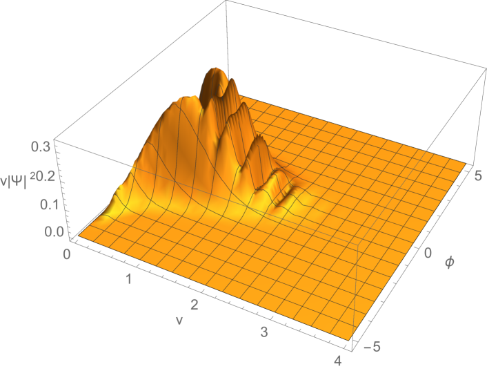
(a) $v|\Psi|^{2}$ for $\omega_{0}/\sigma_{\omega}=10$, $s=1$

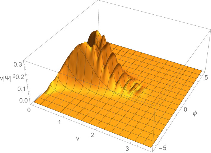
(b) $v|\Psi|^{2}$ for $\omega_{0}/\sigma_{\omega}=15$, $s=1$

Figure 1: Comparison of Born amplitude at bounce time for different choices of $\omega_{0}$ and $s$ (for $\sigma_{\omega}=\sigma_{k}=\hbar=1$).

The parameter $k_{0}/\sigma_{k}$ controls how tightly the individual envelopes stay peaked on the classical solutions. This can be studied by varying the parameter $s=k_{0}/\omega_{0}$ for fixed $\omega_{0}/\sigma_{\omega}$ and $k_{0}/\hbar$ and parametrically plotting $\left\langle\hat{v}\right\rangle/s$ and $\left\langle\hat{\varphi}\right\rangle$. The advantage of this choice of parameterization of the quantum solutions in terms of $s$ is that the classical equations of motion can be written parametrically as

$$\frac{v}{s}=\left|\text{cosech}\left(\varphi-\varphi_{\infty}\right)\right|\,.$$ (22)

The quantum curve for different choices of $s$ can thus be compared with the same universal classical curve. FIG 2 illustrates the relevant features. The expectation values begin to diverge from their classical values in the region $v\sim 1/\sigma_{\omega}$ as expected. The expectation value of $\hat{\varphi}$ reaches a maximum value, which increases as $s$ increases. The expectation value of $\hat{v}$ reaches a minimum at $t=0$ as expected.

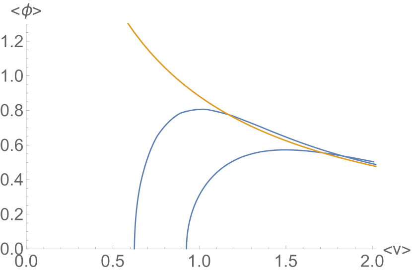
Figure 2: $\left\langle\hat{v}\right\rangle/s$ versus $\left\langle\hat{\varphi}\right\rangle$ for different $s$ and $\omega_{0}=10$. Top blue: $s=1$; bottom blue: $s=2$; yellow: classical. (Symmetric upon $\varphi\to-\varphi$.)

VIII Prospectus

Let us briefly consider potential connection between the model and inflationary cosmology. In particular, following PhysRevD.42.3936 ; Liddle:1994dx , it is possible to define effective slow-roll parameters using the implicit dependence of the expectation value of the Hubble parameter as a function of $\left\langle\hat{\varphi}\right\rangle$. This effective Hubble parameter is proportional to $\left\langle\hat{\pi}_{v}\right\rangle$ and therefore the relevant slow-roll parameters are proportional to the first and second derivatives of $\left\langle\hat{\pi}_{v}\right\rangle$. Because $\left\langle\hat{\pi}_{v}\right\rangle$ is bounded, the fact that it is zero at the bounce and decreasing to a positive constant at late times implies that it must have a maximum at some point in the epoch that takes place after the bounce and before the semi-classical regime. This maximum should be similar to the maximum seen in $\left\langle\hat{\varphi}\right\rangle$ in FIG. 2. Near this maximum, the condition for the first slow-roll parameter is satisfied. Because it is possible in our model to arbitrarily widen the width of the wavefunction in $v$-space near the bounce by taking increasingly narrow distributions of the cosmological constant, there may be enough freedom in the parameter space of our model to extend the second rate of change of $\left\langle\hat{\pi}_{v}\right\rangle$ near this maximum so that the condition for the second slow-roll parameter is also satisfied. This would be similar to how the second rate of change of $\left\langle\hat{\varphi}\right\rangle$ can be slowed near its maximum by increasing $s$ as can be seen in FIG. 2. The Rayleigh limit also suggests that this potential inflationary regime could be found to take place far below the Planck energy. This raises the exciting possibility, to be pursued in future work, of describing inflationary scenarios using the model.

A further extension of our work is a unitary quantization of anisotropic Bianchi models wainwright_ellis_1997 . While the extension to Bianchi I is straightforward, Bianchi IX models will lead to modifications of the Bessel equations. This notwithstanding, one may expect that many of the qualitative features of the present model will carry forward to solutions of the Bianchi IX model that persist to the late-time attractors. The Bianchi IX model may be particularly valuable for studying general singularity resolution in quantized GR in light of the BKL conjecture Belinsky:1970ew . Such a framework may be useful for studying singularity resolution of time-like singularities via, for example, black-to-white hole transitions.

IX Acknowledgments

We are appreciative to audiences in Bristol, Berlin, Geneva, Harvard, Hannover, Nottingham and the Perimeter Institute for comments. We also thank Henrique Gomes, David Sloan, and Martin Bojowald for helpful comments. We are very grateful for the support from the Institute for Advanced Studies and the School of Arts at the University of Bristol and to the Arts and Humanities Research Council (Grant Ref. AH/P004415/1). S.G. would like to acknowledge support from the Netherlands Organisation for Scientific Research (NWO) (Project No. 620.01.784) and Radboud University. K.T. would like to thank the Alexander von Humboldt Foundation and the Munich Center for Mathematical Philosophy (Ludwig-Maximilians-Universität München) for supporting the early stages of work on this project.

References

- (1) S. W. Hawking and G. F. R. Ellis, The large scale structure of space-time, vol. 1. Cambridge university press, 1973.
- (2) R. Brandenberger and P. Peter, “Bouncing cosmologies: progress and problems,” Foundations of Physics 47 no. 6, (2017) 797–850.
- (3) C. Isham, “Canonical quantum gravity and the problem of time,” Arxiv preprint gr-qc (1992) . http://arxiv.org/abs/grqc/9210011.
- (4) K. Kuchar̆, “The problem of time in canonical quantization of relativistic systems,” in Conceptual Problems of Quantum Gravity, A. Ashtekar and J. Stachel, eds., p. 141. Boston University Press, 1991.
- (5) E. Anderson, “Problem of time in quantum gravity,” Annalen der Physik 524 no. 12, (2012) 757–786.
- (6) S. Gryb and K. P. Y. Thébault, “The role of time in relational quantum theories,” Foundations of Physics (2011) 1–29.
- (7) S. Gryb and K. P. Y. Thébault, “Symmetry and evolution in quantum gravity,” Foundations of Physics 44 no. 3, (2014) 305–348.
- (8) S. Gryb and K. P. Y. Thébault, “Schrödinger Evolution for the Universe: Reparametrization,” Classical and Quantum Gravity 33 no. 6, (2016) 065004.
- (9) C. Rovelli, “Partial observables,” Phys. Rev. D 65 (2002) 124013.
- (10) B. Dittrich, “Partial and complete observables for hamiltonian constrained systems,” General Relativity and Gravitation 39 (2007) 1891.
- (11) R. Gambini, R. A. Porto, J. Pullin, and S. Torterolo, “Conditional probabilities with dirac observables and the problem of time in quantum gravity,” Physical Review D 79 no. 4, (2009) 041501.
- (12) J. Barbour and B. Z. Foster, “Constraints and gauge transformations: Dirac’s theorem is not always valid,” ArXiv e-prints (Aug., 2008) , arXiv:0808.1223 [gr-qc].
- (13) J. Pons, “On dirac’s incomplete analysis of gauge transformations,” Studies In History and Philosophy of Science Part B: … 36 (2005) 491.
- (14) J. Pons, D. Salisbury, and K. A. Sundermeyer, “Observables in classical canonical gravity: folklore demystified,” Journal of Physics A: Mathematical and General 222 no. 12018, (2010) .
- (15) M. Bojowald, “Absence of a singularity in loop quantum cosmology,” Physical Review Letters 86 no. 23, (2001) 5227.
- (16) A. Ashtekar, A. Corichi, and P. Singh, “Robustness of key features of loop quantum cosmology,” Physical Review D 77 no. 2, (2008) 024046.
- (17) W. G. Unruh and R. M. Wald, “Time And The Interpretation Of Canonical Quantum Gravity,” Phys. Rev. D40 (1989) 2598.
- (18) W. G. Unruh, “A Unimodular Theory Of Canonical Quantum Gravity,” Phys. Rev. D40 (1989) 1048.
- (19) S. Gielen and N. Turok, “Perfect quantum cosmological bounce,” Physical Review Letters 117 no. 2, (2016) 021301.
- (20) S. Gielen and N. Turok, “Quantum propagation across cosmological singularities,” Phys. Rev. D95 no. 10, (2017) 103510, arXiv:1612.02792 [gr-qc].
- (21) S. Gryb and K. P. Y. Thébault, “Bouncing Unitary Cosmology I: Mini-Superspace General Solution,” arXiv:1801.05789 [gr-qc].
- (22) S. Gryb and K. P. Y. Thébault, “Bouncing Unitary Cosmology II: Mini-Superspace Phenomenology,” arXiv:1801.05826 [gr-qc].
- (23) C. J. Isham, “Topological and global aspects of quantum theory,” in Relativity, groups and topology. 2. 1984.
- (24) M. Reed and B. Simon, Methods of Modern Mathematical Physics II: Fourier Analysis, Self-Adjointness, vol. 2. Elsevier, 1975.
- (25) M. Reed and B. Simon, Methods of modern mathematical physics. vol. 1. Functional analysis. Academic, 1980.
- (26) V. Husain and O. Winkler, “Singularity resolution in quantum gravity,” Physical Review D 69 no. 8, (2004) 084016.
- (27) M. Bojowald, “Singularities and quantum gravity,” arXiv preprint gr-qc/0702144 (2007) .
- (28) C. Kiefer, Quantum Gravity. International Series of Monographs on Physics. Clarendon Press, Oxford,, 2007.
- (29) D. Brizuela, “Statistical moments for classical and quantum dynamics: formalism and generalized uncertainty relations,” Physical Review D 90 no. 8, (2014) 085027.
- (30) C. Kiefer and H. Zeh, “Arrow of time in a recollapsing quantum universe,” Physical Review D 51 no. 8, (1995) 4145.
- (31) D. S. Salopek and J. R. Bond, “Nonlinear evolution of long-wavelength metric fluctuations in inflationary models,” Phys. Rev. D 42 (Dec, 1990) 3936–3962.
- (32) A. R. Liddle, P. Parsons, and J. D. Barrow, “Formalizing the slow roll approximation in inflation,” Phys. Rev. D50 (1994) 7222–7232, arXiv:astro-ph/9408015 [astro-ph].
- (33) J. Wainwright and G. Ellis, eds., Dynamical Systems in Cosmology. Cambridge University Press, 1997.
- (34) V. A. Belinsky, I. M. Khalatnikov, and E. M. Lifshitz, “Oscillatory approach to a singular point in the relativistic cosmology,” Adv. Phys. 19 (1970) 525–573.