Flux cost functions and optimal metabolic states

Abstract

The metabolic fluxes in cells follow physical, biochemical, and economic principles. Some flux balance analysis (FBA) methods trade flux benefit against flux cost. However, if flux cost functions are linear and meant to describe underlying enzyme costs, this entails that enzyme efficiencies are constant and ignores the interplay between fluxes, metabolite concentrations and enzyme levels in cells. Here I introduce realistic flux cost functions that describe an “overhead cost”, namely the minimum enzyme and metabolite cost associated with the fluxes in a kinetic model. These flux cost functions have general mathematical properties. Enzymatic flux cost functions, which represent enzyme costs, scale proportionally with the flux profile and are concave on the flux polytope. Kinetic flux cost functions represent the sum of enzyme and metabolite costs. If two flux profiles are superimposed, their different demands for metabolite concentrations cause an extra compromise cost, which makes flux cost functions strictly concave in almost all cases. When fluxes change their direction, the enzymatic cost jumps abruptly. Based on general flux cost functions, I propose two methods for flux modelling: Flux Cost Minimisation, a nonlinear variant of FBA with flux minimisation, and Flux Benefit Optimisation, a nonlinear variant of FBA with molecular crowding. The optimal flux profiles, at a given flux benefit, are vertices of the flux polytope. In models without other flux constraints, these vertices are elementary flux modes. Linear approximations of enzymatic flux cost can be used in FBA. In contrast to flux costs chosen ad hoc, these functions reflect the enzyme kinetics and extracellular concentrations in realistic kinetic models. Based on enzymatic flux costs, we can describe the cell growth rate as a convex function on the flux polytope and derive growth-optimal metabolic states and statistical distributions for the fluxes in cell populations. Therefore, flux cost functions unify kinetic models and flux analysis, provide parameters for FBA models, and shows that these models are physically justified.

Keywords: Flux balance analysis, enzyme cost, metabolite cost, concave function, elementary flux mode.

Abbreviations: ECM: Enzyme Cost Minimisation; FCM: Flux Cost Minimisation; FBA: Flux Balance Analysis; CM: Common Modular rate law; mfFBA: FBA with minimal fluxes; mwfFBA: FBA with minimal weighted fluxes; mcFBA: FBA with molecular crowding; CAFBA: constrained allocation FBA; RBA: Resource Balance Analysis

1 Introduction

The metabolic state of a cell, consisting of metabolic fluxes, metabolite concentrations, and enzyme levels, is constantly adapted to external conditions and cellular demands. Since the aim of metabolism is substance conversion, the metabolic fluxes are the main variables to be controlled. Which metabolic pathways should a cell use in a given environment, and how should pathway fluxes be adjusted to varying nutrient supply? When should pathways be switched on or off? Which enzyme and metabolite concentrations belong to a flux profile, and more generally, how do enzyme and metabolite costs affect the choice between flux profiles?

To predict metabolic strategies, we may first ask what fluxes are physically possible. In Flux Balance Analysis (FBA), flux profiles are required to respect flux bounds, be stationary (i.e. mass-balanced internal metabolites), and possibly show thermodynamically feasible flux directions. But which of the possible flux profiles will be realised by cells, depending on enzyme parameters and environmental conditions? Kinetic models explain metabolic fluxes by rate laws, enzyme levels, and metabolite concentrations. But even if all rate laws were known, these predictions would be uncertain because enzyme and metabolite concentrations are highly variable. Flux analysis models work differently: they assume that cells choose, among all physically feasible flux profiles, the most profitable one, e.g. the one that provides the best compromise between biomass production rate (benefit) and total enzyme demand (cost). The idea is simple: just like the efficiency of a single enzyme (the flux per enzyme level), the overall catalytic rate of metabolism (the biomass production per total metabolic enzyme) may be optimised. A cost-efficient metabolism can be useful both for fast growth and for allocating protein resources to other tasks, at a given growth rate or even in non-growing cells.

Figure 1: Metabolic flux profiles, flux cost, and optimal fluxes. (a) Fluxes in central metabolism. Three basic flux profiles (for pure fermentation, respiration, and respiration on ethanol) and a convex combination of them (respiro-fermentation) are shown. With ATP production (small circles) as a benefit function, all flux profiles can be scaled to a unit benefit value (i.e. unit ATP production rate). For simplicity, ethanol uptake is described as a reverted ethanol overflow (using the same enzyme). (b) Flux profiles as points in flux space, spanned by the reaction fluxes $v_{1}$, $v_{2}$ and $v_{3}$. The plane of stationary fluxes is defined by the constraint $v_{1}=v_{2}+v_{3}$. The feasible flux profiles with given flux directions form a convex polytope ${\mathcal{P}}_{\rm F}$. On the right, two such polytopes (for varying directions of the ethanol excretion flux) are shown. (c) Flux profiles as points in flux space (projection on the $v_{2}/v_{3}$ plane). Flux profiles with unit ATP production lie on a diagonal line (called B-polytope and shown in light blue). (d) Each flux profile defines a set of feasible metabolite profiles, forming a convex polytope in log-metabolite space (called M-polytope). Given a desired flux profile, each metabolite profile requires a particular enzyme profile with a particular cost, which can be an effective metabolite cost function on the M-polytope. Minimising this function yields an optimal metabolite profile, an optimal enzyme profile, and a minimal cost value called enzymatic flux cost. (e) Enzymatic flux cost as a function on the flux polytope. The enzymatic cost $a^{\rm enz}({\bf v})$ is defined as the minimum enzyme cost at which a flux profile can be realised in a given kinetic model. The flux profile with the smallest cost on the B-polytope is assumed to be optimal. (f) A bound on respiration (flux bound shown by dashed line) gives rise to a new vertex point, describing respiro-fermentation. (g) In the (schematic) example show, respiro-fermentation is the optimal strategy.

Cost-benefit optimisation is a common approach in economics and also in flux prediction. Constraint-based modelling (CBM) methods such as Flux Balance Analysis [1] or Resource Balance Analysis [2] constrain metabolic fluxes by assuming a steady state and imposing linear flux bounds. Then, a flux benefit can be maximised or a flux cost is minimised at a fixed benefit. Under these constraints, flux costs can then be constrained or minimised. In classical FBA, there are separate bounds on single fluxes (an assumption without a good physical justification, unless individual enzyme levels are known). Internal cycle fluxes, which have no effect on the benefit, remain undetermined and can lead to underdetermined, unrealistic flux solutions. To avoid this, other FBA methods constrain or penalise fluxes more generally. In FBA with molecular crowding (mcFBA) [3], each flux profile is associated with an enzyme demand, written as a weighted sum of the absolute fluxes (or the fluxes themselves, if fluxes are known to be positive). This enzyme demand is then bounded (e.g. to account for limited space in the cell; hence the name “FBA with molecular crowding”). FBA with flux minimisation (mfFBA) [4] does exactly the opposite: flux costs (described by a possibly weighted sum of absolute fluxes) are not bounded during optimisation, but are themselves minimised (at a given flux benefit). Both methods can predict sparse flux profiles in which only the most profitable pathways are active. To justify linear flux cost functions or linear flux constraints, it is assumed that fluxes are proportional to enzyme levels with constant proportionality factors (called catalytic rates, apparent catalytic constants, or enzyme efficiencies) [5].

, In reality, the enzyme efficiencies are not constant, but depend on metabolite concentrations and vary between metabolic states of the cell. Enzyme levels and stationary fluxes are not simply proportional! Proportionality holds if metabolite concentrations are constant, but this is usually not the case: when enzyme levels are changing, this changes both steady-state fluxes, metabolite concentrations, and enzyme efficiencies. The enzyme catalytic rates play a key role in determining metabolic strategies. In FBA with molecular crowding, they serve as the conversion factors between enzyme levels and fluxes. A linear conversion from fluxes to enzyme levels assumes that enzymes work at a constant catalytic rate (approximated by the $k_{\rm cat}$ value or by a smaller “catalytic rate” $k_{\rm app}$), thus ignoring enzyme kinetics. In kinetic models, enzyme efficiencies depend on metabolite concentrations, as described by the rate laws – and since metabolite concentrations vary, the efficiencies vary as well! In FBA models based on resource allocation (like FBA with minimal fluxes, FBA with molecular crowding, or CAFBA ), the enzyme efficiencies are important parameters: they determine the choice of fluxes, metabolic strategies, and growth rates. The biomass/enzyme productivity (i.e. the biomass production rate per amount of metabolic enzyme) also plays an important role in protein allocation models (e.g. used to explain bacterial growth laws [6]), which can be used to relate the biomass/enzyme productivity to cell growth rates (as shown in [7] and below in this article). Thus, enzyme efficiencies are important. If they depend on metabolite concentrations, if metabolite concentrations depend on the metabolic state, and if the enzyme levels in optimal states depend again on enzyme effiencies, all these variables need to be found at the same time and the relation between fluxes and enzyme levels will be complicated. The complex interplay between all these variables and its consequences for flux prediction are addressed in this paper.

So, let us open Pandora’s box and predict fluxes, metabolite concentrations, and enzyme levels at the same time. To optimise all of them, we combine flux modelling with underlying kinetic models and perform a layered optimisation: first, given a predefined flux distribution, we optimise enzyme and metabolite concentrations; by solving this problem, we can associate our flux profile with an effective (enzyme and metabolite) cost, summarising all details of the kinetic model (both optimality and kinetics) in a nonlinear flux cost function. By associating each flux profile with a cost, we can find an optimal flux profile by minimising this cost function in flux space. The result is an optimal flux profile together with its optimal enzyme and metabolite concentrations and the corresponding enzyme efficiencies. Altogether, this method resembles a minimal-flux FBA with a flux cost function obtained by solving an optimality problem for enzyme and metabolite concentrations. This latter problem, a search for optimal enzyme levels that minimise the overall enzyme demand [8, 9] is called enzyme cost minimisation (ECM) [10] and can be reformulated as a convex optimisation over metabolite profiles. In ECM , different flux modes favour different metabolite concentrations and therefore different enzyme efficiencies. This leads to nonlinear relationships between fluxes and enzyme cost. In this article, we consider flux cost functions $a({\bf v})$ more generally and study their mathematical properties. We describe nonlinear variants of FBA based on these functions (FCM and FBM), and draw conclusions for cellular growth rates and the probabilities of metabolic states in cell populations.

In FBA models, flux cost can either be minimised (as in minimal-flux FBA) or constrained (as in FBA with molecular crowding). Assuming nonlinear flux cost functions, I propose two methods for flux prediction called Flux Cost Minimisation (FCM) and Flux Benefit Maximisation (FBM). Both methods lead to concave optimality problems [11, 7]. In FCM, we search for flux distributions that minimise flux cost at a given flux benefit (e.g. a given rate of biomass production). Applied to metabolism as a whole, it yields the ratio of biomass production and enzyme cost. This biomass/catalytic rate (or “enzyme productivity”) is an important quantity in protein allocation models [6], where it determines the achievable growth rate of cells. This approach – minimising the enzyme cost per biomass production rate, computing the resulting cost/benefit ratio, and translating it into cellular growth rates – has previously been applied to a model of central metabolism [7].

Importantly, under certain assumptions the optimal flux solutions are elementary flux modes. This had been proven for similar optimality problems (e.g. maximising a linear flux benefit at a given total enzyme amount) [11, 12]: in these problems, the enzyme cost per flux is a concave function in flux space, and it was shown that optimal flux profiles must be elementary flux modes (EFMs), no matter which underlying kinetic model is assumed.

Here I discuss how flux cost functions can be defined, what are their mathematical properties, and how they can be used in modelling. The functions allow us to represent different types of biological costs as costs in flux space, in order to, then, simply optimise over the flux distributions. I first show how enzyme and metabolite costs can be written as flux cost functions, and how such functions reflect the underlying kinetic models and optimality principles. Then I study the mathematical properties. Unlike flux cost functions FBA, they need not be linear: when two flux modes are superimposed, their costs may not add up, but there may be an extra compromise cost, that makes the function strictly concave. Based on these mathematical properties, I discuss how enzymatic and kinetic flux cost functions can be used for flux prediction and to define linearised cost functions for FBA, how predicted enzyme demands can be converted into cell growth rates [6], and how we can compute probability distributions of metabolic states in cell populations. This connects metabolic models to cell or population models The running example in this article is a simple branch point model like in figure 1, but all concepts apply to metabolic networks of any size.

2 Flux costs scoring enzyme and metabolite concentrations

2.1 Enzymatic and kinetic flux cost functions

A cell can realise a flux profile ${\bf v}$ by different combinations of enzyme and metabolite concentrations. High concentrations are costly: in experiments, overexpressing an idle protein reduces cell growth. In the case of enzymes, the same costs may exist and may counterbalance the effects of the higher catalysed fluxes [13, 14]. An explanation for this growth deficit is that material resources and cell space are limited and that, therefore, higher enzyme or metabolite concentrations in one pathway imply lower protein concentrations, and therefore a lower performance, in other pathways, which compromises cell growth. To model this, fluxes may be penalised by effective flux cost functions or may be constrained by $k_{\rm cat}\cdot e$, the product of catalytic constant $k_{\rm cat}$ and enzyme level $e$ to be bounded or minimised. In flux modelling, enzyme costs can be taken into account in several ways. Molecular Crowing FBA [3] assumes that each flux profile requires some overall enzyme amount, which is bounded due to limited space in cells. To translate fluxes into enzyme amounts, a simple linear relationship is used. FBA with molecular crowding (mcFBA) [4] works similarly: after predefining a required flux benefit ($b=\sum_{l}b_{v_{l}}^{\prime}\,v_{l}$), one minimises a sum $a=\sum_{l}|v_{l}|$ or a weighted sum of fluxes $a=\sum_{l}a_{v_{l}}|v_{l}|$ with cost weights $a_{v_{l}}$ (where flux signs are ignored). Again, these flux costs may represent enzyme costs. In classical FBA, metabolic flux profiles are predicted by assuming a linear benefit function $b={\bf b}_{v}^{\prime}\cdot\,{\bf v}$ (e.g. the biomass production rate) and maximising this benefit on the flux polytope. More generally, in FBA methods, maximisation of flux benefit (e.g. biomass production) and minimisation of flux cost (e.g. the sum of absolute fluxes) can be combined in different ways, e.g. by layered optimisation [4] or multi-criteria optimisation [15, 16].

In all these methods, we assume that fluxes and enzyme levels are strictly proportional, which leads to linear flux cost functions. Moreover, enzymes are sometimes assumed to operate at their maximal rate (called $k_{\rm cat}$ value), and deviations from this ideal assumption have been dubbed “unused enzyme capacity” [17]. However, part of this “unused capacity”is due to the fact that the enzymes within a larger network cannot operate at their maximal speed, so we need to beware of idealised models that ignore the trade-offs between enzymes and underpredict the enzyme demands! If flux cost weights for FBA are computed from $k_{\rm cat}$ values, these are lower bounds on the actual cost weights and the actual values remain unclear. All this is of course unrealistic. To address these problems, we now define realistic flux cost functions which reflect the minimal enzyme and metabolite costs that come with the fluxes in a given kinetic model (Figure 1). Both types of cost have been considered before (enzyme costs in [18, 8, 19], enzyme plus metabolite costs in [20, 21]). To write them as flux costs, we first need to score enzyme levels, metabolite concentrations, and fluxes by cost and benefit functions: enzyme cost is a linear function of enzyme levels (i.e. penalising high enzyme levels), metabolite cost is a convex function of the logarithmic metabolite concentrations (e.g. penalising deviations from some ideal metabolite profile), and flux benefit is a linear function of the fluxes. Given these metabolic targets, we may formulate different optimality problems: we may assume that cells maximise either the benefit-cost difference, the benefit/cost ratio, or the benefit at a fixed cost, or that they minimise cost at a fixed benefit. Below, we mostly consider this latter case, where “cost” can refer to enzyme cost or the sum of enzyme and metabolite costs. having all this in place, we can finally assign to each flux profile the metabolite and enzyme profiles that can realise this flux profile in the most beneficial way, quantify these profile by their cost functions and assign this cost as an effective “flux cost” to our metabolic flux profile.

Box 1: Cost functions for enzymes, metabolites, and fluxes in cells
The fluxes $v$, metabolite concentrations $c$, and enzyme levels $e$ in cells depend on each other. An enzyme cost $h({\bf e})$, a function of the enzyme levels, can be translated into an effective metabolite cost or a flux cost. We obtain three different variants of our cost function enzyme cost function, with different cell variables as function arguments
1. Enzyme cost An enzyme cost function $h(e_{1},e_{2},..)$ is assumed to score enzyme levels directly. If each enzyme molecule has a fixed cost (which may differ between enzymes), we obtain a linear enzyme cost function. The meaning and physical units of enzyme cost functions may vary from model to model. A cost may, for example, refer to enzyme amounts (e.g. enzyme mass per cell dry weight), e.g. when predicting the enzyme demand of engineered pathways, or to overall growth defects in units of 1/h (for absolute growth rate changes) or unitless (for relative growth rate changes).
2. Metabolite cost (or “flux-restricted enzymatic M-cost”) A given flux profile defines thermodynamic constraints on the possible metabolite concentrations. The feasible metabolite profiles form a convex polytope in log-concentration space, called metabolite polytope or M-polytope. Its shape depends on network structure and flux directions, equilibrium constants, and external metabolite concentrations (see [10]). Metabolite cost is described by functions on this polytope. The enzymatic M-cost $\displaystyle g^{\rm enz}({\bf m};{\bf v})=h(\mathbf{e}({\bf v},{\bf m}))$ (1) is an effective (or “overhead”) cost, describing the enzyme cost $h(\mathbf{e})$ needed to realise a flux profile ${\bf v}$ at the metabolite profile ${\bf m}=\ln{\bf c}$, with given external metabolite concentrations and within allowed ranges for internal metabolite concentrations. Given a flux profile ${\bf v}$, the enzyme levels $\mathbf{e}({\bf v},{\bf m})$ follow directly from the kinetic rate laws. The cost (1) is a convex function of log-concentrations [10], and the optimal metabolite profile can be computed by convex optimisation (see Figure 1), defining the optimal enzyme profile and enzyme cost. By adding a direct metabolite cost $g({\bf m})$, we obtain the kinetic metabolite cost $\displaystyle g^{\rm kin}({\bf m})=g({\bf m})+g^{\rm enz}({\bf m}).$ (2) The metabolite cost g(m) should be convex (or even strictly convex) of mathematical convenience. It may describe, for example, the total metabolite mass density or a quadratic deviation from an (empiricall or biologically) preferred metabolite profile. If $g({\bf m})$ is strictly convex, the kinetic metabolite cost has be strictly convex and will have a unique optimum point, uniquely defining optimal enzyme and metabolite concentrations.
3. Flux cost (or “metabolite-optimised enzymatic F-cost”) The enzymatic flux cost $\displaystyle a^{\rm enz}({\bf v})=\mbox{min}_{\bf m}\,g^{\rm enz}({\bf m};{\bf v})=\mbox{min}_{\bf m}\,h(\mathbf{e}({\bf v},{\bf m}))$ (3) is the minimal enzyme cost at which we can realise the flux profile ${\bf v}$ in a given kinetic model (see Figure 1). If we add a direct metabolite cost, we obtain the kinetic flux cost $\displaystyle a^{\rm kin}({\bf v})=\mbox{min}_{\bf m}\,g^{\rm kin}({\bf m}|{\bf v}),$ (4) i.e. the minimal sum of enzyme and metabolite costs at which ${\bf v}$ can be realised in our model. Flux cost functions $a({\bf v})$ can also be defined ad hoc (like the linear cost functions in FBA), In any case, they should increase with the absolute flux for plausibility reasons (satisfying $\mbox{sign}(\partial a/\partial v_{l})=\mbox{sign}(v_{l})$ whenever $v_{l}\neq 0$), and they may show a jump where a reaction flux $v_{l}$ switches its sign, i.e. where $v_{l}=0$.

How can we find an optimal metabolic state, comprising metabolite concentrations, enzyme levels, and fluxes? While each flux profile requires certain metabolite and enzyme profiles for its realisation, this choice is not unique. Each flux profile can be realised by different combinations of enzyme and metabolite concentrations. To choose the best concentration profiles, we assume that cells minimise their enzyme cost [19, 10] or their “kinetic” (i.e. enzyme plus metabolite) cost, where costs may represent, for example, occupied cell volume or molecular mass. By conceptualising enzyme and metabolite costs as flux costs, we can translate kinetic optimality problems into a simple search for optimal fluxes. Enzyme and metabolite concentrations are not mentioned explicitly, but their costs are implicitly taken into account. With this optimality principle, each flux mode defines an optimal metabolite and enzyme profile. Importantly, these profiles are not required by the flux profile (because other profiles would yield the same fluxes), but favoured by it, because they are less costly than other (physically and biochemically) possible choices. The cost of these profiles can be seen as the “overhead flux cost”, i.e. a cost that is not caused by the fluxes themselves, but are inevitable if the fluxes are to be physically realised! By minimising this flux cost function, we optimise the entire metabolic state, including fluxes, metabolite concentrations and enzyme levels.

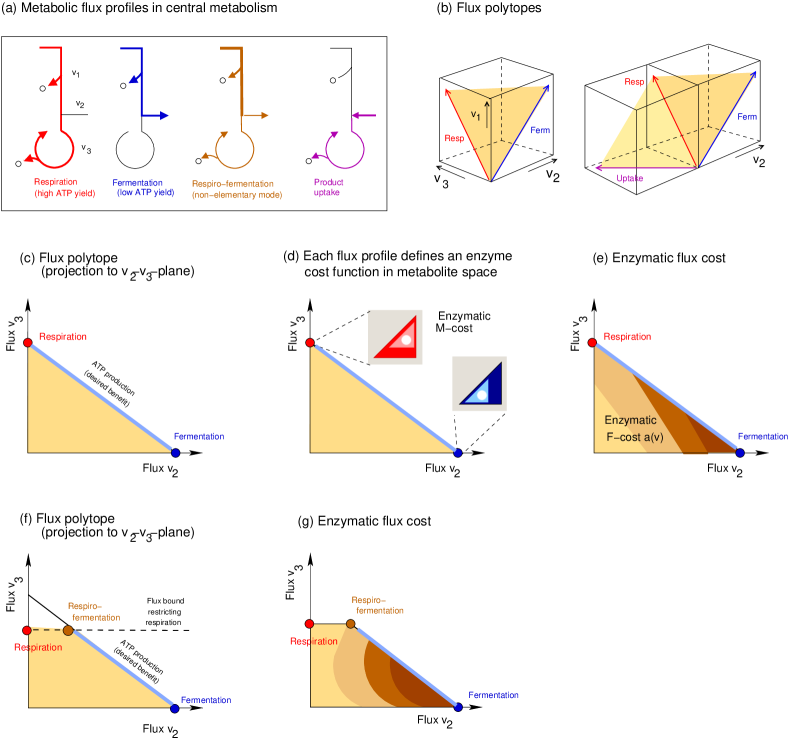
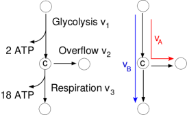
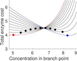
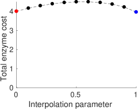
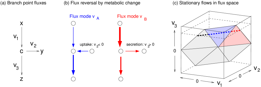
Let us see an example. Figure 2 shows a simple model of central metabolism, describing the choice between overflow metabolism and respiration (compare Figure 1 (a)). We assume reversible mass-action rate laws and fluxes in forward direction. Given the fluxes $v_{l}$, the enzyme cost can be written as a function of the logarithmic metabolite concentration $m=\ln c$. We obtain the formula $g(m)=\frac{a_{0}}{b_{0}-e^{m}}v_{0}+\frac{a_{1}\,e^{m}}{e^{m}-b_{1}}v_{1}+\frac{a_{2}\,e^{m}}{e^{m}-b_{2}}v_{2}$. In our model, any stationary flux distribution is a combination of two basic flux profiles. In the first profile, the entire flux goes through the overflow reaction; in the second one, the entire flux goes through respiration. Since the flux directions are fixed, any other flux profiles, with different flux ratios, must be convex combinations of these basic profiles. Figure 2 (b) and (c) show enzyme cost as a function in metabolite space and in flux space. In metabolite space, the blue and red lines denote the costs for the basic flux profiles, and the minimum cost for a combined flux profile must lie in between these two lines. The overall minimum cost is always achieved by one of the basic flux profiles (blue dot for ${\bf v}_{\rm B}$ in the example shown).

(a) Branch point model	(b) Enzyme cost in metabolite space	(c) Enzyme cost in flux space

Figure 2: Enzymatic flux cost in a branch point model of fermentation and respiration. (a) Model of central metabolism (see Figure 1) with reactions representing glycolysis ($v_{1}$), overflow ($v_{2}$), and respiration ($v_{3}$). The internal metabolite C (e.g. pyruvate) has a variable concentration $c$, while all other concentrations are fixed. We consider a kinetic model with substrate-saturated, reversible rate laws and a linear benefit function $b(v_{1},v_{2},v_{3})$ scoring the ATP production rate. All stationary flux profiles are convex combinations of two basic profiles ${\bf v}_{\rm A}$ (respiration, red) and ${\bf v}_{\rm B}$ (fermentation, blue). (b) Enzymatic cost in metabolite space. Cost functions for the basic flux profiles ${\bf v}_{\rm A}$ and ${\bf v}_{\rm B}$ (scaled to equal ATP production rates) are shown by red and blue lines. Black lines show cost functions for combined flux profiles $\sigma\,{\bf v}_{\rm A}+(1-\sigma)\,{\bf v}_{\rm B}$, interpolating between ${\bf v}_{\rm A}$ and ${\bf v}_{\rm B}$. For each flux profile, the optimum point is shown by a dot. (c) Enzyme cost in flux space. The optimal costs from (b) are plotted as a function of the interpolation parameter $\sigma$, which varies between 0 (for flux profile ${\bf v}_{\rm A}$) to 1 (for flux profile ${\bf v}_{\rm B}$). The resulting cost function $a^{\rm enz}({\bf v})$ is negatively curved and therefore strictly concave.

2.2 Shape of the enzymatic cost flux function

Enzymatic flux costs can be computed by numerical optimisation, but there is no closed formula to describe them. So what are their mathematical properties? The enzymatic flux cost $a^{\rm enz}({\bf v})$ is a nonlinear function defined on the set of thermodynamically feasible flux profiles. Its precise shape depends on rate laws, parameters, external conditions, and constraints of the kinetic model. In the following I consider models with biochemically plausible rate laws such as the common modular (CM) rate law, which has convenient mathematical properties. More specifically, we consider factorised rate laws [24], which comprise all plausible reversible rate laws and ensure thermodynamically correct reaction directions. I further assume that enzyme cost depends linearly on enzyme levels (for more details about models and their mathematical description, see the SI).

The cost of metabolic flux distributions can be described by a cost function in flux space. To describe these functions, as well the set of feasible flux distributions, we need some precise terminology. Stationary flux distributions are called flux profiles, or flux modes (if their scaling does not play a role). A flux pattern $\mbox{sign}({\bf v})$ is a vector describing the actual flux directions in a flux profile ${\bf v}$ (with elements -1, 0, and 1). A flux template ${\boldsymbol{\sigma}}$ is a sign vector that defines allowed flux directions (where fluxes may always vanish). A flux distribution ${\bf v}$ is conformal with ${\boldsymbol{\sigma}}$ if $\mbox{sign}(v_{l})=\sigma_{l}$ for all $v_{l}\neq 0$. Flux templates may follow, for example, from thermodynamic driving forces, which in turn depend on the chemical potentials (and therefore on metabolite concentrations).

Geometrically, a flux profile can be seen as a point in a flux space (Figure 1). The set of feasible flux profiles is defined by model constraints, including stationarity, predefined flux directions and inactive reactions, bounds on fluxes or flux sums, or a predefined flux benefit. How will these constraints shape the set of feasible flux profiles? First, the stationarity condition defines a linear subspace in flux space. Second, a given flux template predefines zero fluxes in some of the reactions and flux directions in others, defining a feasible segment in flux space. The intersection of stationarity constraints and sign constraints yields a flux cone. If all flux directions are definedm the cone is inside of one of the orthants. Instead of imposing flux directions directly, we may require that the flux directions follow thermodynamic constraints. Given the equilibrium constants and external metabolite concentrations, only some flux sign profiles remain thermodynamically feasible (see Box 3). Each of them defines a feasible segment in flux space. Third, individual flux bounds define a feasible box in flux space. Fourth, space limitations may put constraints on the total enzyme levels in cell compartments. In mcFBA, this density constraint leads to upper bounds on weighted sum of fluxes. Fifth, we may score our flux profiles by a linear benefit function, for example, the rate of biomass production. By predefining this flux benefit, we exclude some flux profiles (those that provide no or negative benefits) and normalise all others (e.g. to a benefit of 1). Mathematically, this restrict our flux profiles to a feasible hyperplane which intersects the flux cone, giving rise to the so-called B-polytope, whose vertices correspond to EFMs.

These constraints, in different combinations, lead to different variants of FBA. By applying them to our possible flux modes, we limit the flux space to a feasible region, consisting of a collection of convex cones (see Box 3), or convex polytopes if flux bounds are used. Below, the different polytopes (or cones) in this collection will be considered one at a time. As a formal requirement, we assume non-negative fluxes: this is just for convenience, and we can always ensure this by reorienting the reactions. Without any other bounds, we obtain a positively oriented flux cone (called F-cone), and if we add a flux benefit constraint, we obtain the B-polytope.

Having defined a positive flux cone, we can study flux cost functions on this cone. To learn about their shapes, we consider movements between flux profiles (points on the cone) and how they affect flux cost (see Figure 3). A flux cone consists of a “stack” of parallel B-polytopes, each with a different benefit. Any movements between flux profiles consist of two basic types of movement: a rescaling of flux profiles (a movement between B-polytopes) and an interpolation of flux profiles of equal benefit (a movement within a B-polytope). How do these movements affect the flux cost $a^{\rm enz}$? If we scale all fluxes by the same factor $\sigma$, the enzymatic cost scales proportionally (while its flux-specific cost or benefit-specific cost, stays the same). If we interpolate between flux profiles, the cost may vary non-linearly. In general, enzymatic flux costs are concave on the interpolation line, i.e. the cost $a^{\rm enz}({\bf v}_{\rm A}+{\bf v}_{\rm B})$ of a sum of flux profiles can be higher than the sum of costs $a^{\rm enz}({\bf v}_{\rm A})+a^{\rm enz}({\bf v}_{\rm B})$, but not lower. If this superadditive interpolation holds between any two points on a B-polytope, the flux cost functions is strictly concave within the B-polytope.

Figure 3: Enzymatic flux cost function $a^{\rm enz}({\bf v})$ on a flux cone (schematic drawing). (a) Left: a flux cone is spanned by flux modes ${\bf v}_{\rm A}$ and ${\bf v}_{\rm B}$. The cost function (shades of brown) on this cone is concave. Right: The enzymatic cost scales proportionally with the overall flux profile: when a flux profile ${\bf v}$ is scaled by a factor $\sigma$, its enzymatic cost scales linearly, as $a^{\rm enz}(\sigma\,{\bf v})=\sigma\,a^{\rm enz}({\bf v})$. (b) Same as (a), but for movements within a B-polytope (diagonal lines). If two flux profiles ${\bf v}_{\rm A}$ and ${\bf v}_{\rm B}$ are kinetically distinct, i.e. if they favour different metabolite profiles, the cost function on the line between ${\bf v}_{\rm A}$ and ${\bf v}_{\rm B}$ is strictly concave. To obtain a linear cost function instead (dashed line), the cell might run the flux profiles separately, either in space (cell compartments) or in time (phases of a metabolic cycle) Separated in this way, each flux profile can operate under its optimal biochemical conditions and their flux costs are additive.

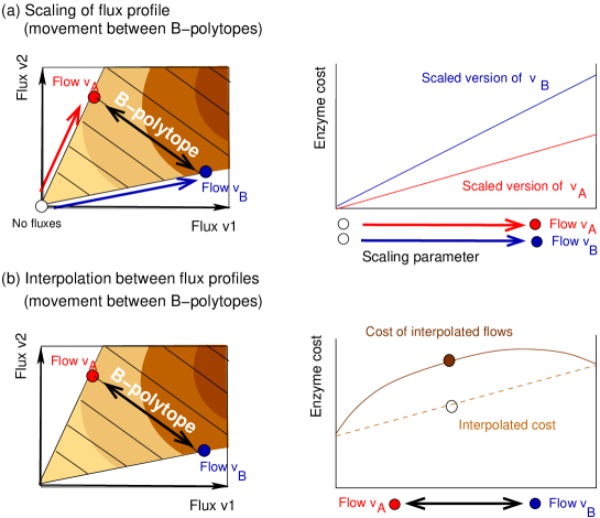
Let us now have a closer look at these properties – proportional scaling and concavity. We start with proportional scaling. With a linear enzyme cost function $h(\mathbf{e})$ and a proportional scaling ${\bf v}\sim{\bf e}$, the flux cost $a^{\rm enz}({\bf v})$ would scale linearly with ${\bf v}$. But why can we assume that metabolite concentrations remain fixed? A given flux profile ${\bf v}$ defines an enzymatic M-cost $g^{\rm enz}({\bf m})$ on the metabolite polytope. If we scale our flux profile ${\bf v}$ by $\sigma$, the function $g^{\rm enz}({\bf m})$ keeps its shape, but is scaled by the same factor $\sigma$. The favoured metabolite profile (i.e. the minimum point of the cost function in metabolite space), stays unchanged, and the favoured enzyme profile keeps its shape, but scales proportionally with the fluxes. Altogether, the enzymatic flux cost $a^{\rm enz}({\bf v})$ scales proportionally with the flux profile and the scaled cost function $\hat{a}^{\rm enz}({\bf v})=a^{\rm enz}({\bf v})/b({\bf v})$ is constant under scaling. Linear scaling leads to useful sum rules (see Box 2) for enzymetic cost functions. What about kinetic flux cost functions $a^{\rm kin}({\bf v})$? If we rescale fluxes and enzyme levels and keep the metabolite levels unchanged, the kinetic M-cost $g^{\rm kin}({\bf m})=g({\bf m})+g^{\rm enz}({\bf m})$, will change linearly with an offset term because $g({\bf m})=\mbox{\rm const.}$ and $g^{\rm enz}({\bf m})=g({\bf e}({\bf v},{\bf c}))$ is proportional to ${\bf v}$. Since this changes the optimal metabolite profile, we cannot expect a simple scaling behaviour for $g^{\rm kin}({\bf m})$.

Box 2: Sum rules for enzymatic flux cost functions
Metabolic steady states have a simple scaling property: if all fluxes are proportionally scaled (e.g. be a time rescaling or a scaling of all enzyme levels) and all metabolite levels stay the same, we obtain again a feasible steady state. In FCM, this scaling has consequences for optimal states. If a flux profile ${\bf v}$ is scaled by a factor $\sigma$ and all external metabolite concentrations stay fixed, the optimal metabolite and enzyme profiles change in a simple way: the metabolite concentrations ${\bf c}^{\rm opt}({\bf v})$ stay constant, while the optimal enzyme levels ${\bf e}^{\rm opt}({\bf v})$ and the enzymatic cost $a^{\rm enz}({\bf v})$ scale proportionally with $\sigma$ (see Figure 3). These scaling properties lead to sum rules for the derivatives of these functions. Since $a^{\rm enz}({\bf v})$ scales proportionally to $\sigma$ with an exponent of 1, it is a homogeneous function of the fluxes with degree 1. Euler’s identity for positive homogeneous functions yields the sum rule $\displaystyle\sum_{l}\frac{\partial a^{\rm enz}}{\partial\ln v_{l}}=a^{\rm enz}.$ (5) By defining the flux investment ${a_{v_{l}}^{\centerdot}}^{\rm enz}=\frac{\partial a^{\rm enz}}{\partial\ln v_{l}}=\frac{\partial a^{\rm enz}}{\partial v_{l}}\,v_{l}$ and the total flux investment ${a_{v}^{\centerdot}}^{\rm enz}=\sum_{l}{a_{v_{l}}^{\centerdot}}^{\rm enz}$, we obtain the equality $\displaystyle{a_{v}^{\centerdot}}^{\rm enz}=a^{\rm enz}.$ (6) In other words: the sum of flux investments is equal to the enzymatic flux cost $a^{\rm enz}$. This holds in each point ${\bf v}$ of the flux cone. We obtain a similar sum rule for the scaled flux cost $\hat{a}^{\rm enz}({\bf v})$ (for example, a flux cost per pathway flux or a flux cost per flux benefit). Since $\hat{a}^{\rm enz}({\bf v})$ is invariant under a scaling of ${\sigma}$ and is therefore a homogeneous function with degree 0, the sum rule reads $\displaystyle\hat{a_{v}^{\centerdot}}^{\rm enz}=\sum_{l}{{\hat{a}_{v_{l}}^{\centerdot}}}\ ^{\rm enz}=\sum_{l}{{\hat{a}_{v_{l}}}}^{\rm enz}\,v_{l}=0.$ (7) There are similar sum rules for optimal metabolite or enzyme levels: $\displaystyle\sum_{l}{e^{\centerdot}}^{j,\rm opt}_{v_{l}}=e^{\rm opt}_{j},\qquad\sum_{l}{c^{\centerdot}}^{i,\rm opt}_{v_{l}}=0,$ (8) where ${e^{\centerdot}}^{j,\rm opt}_{v_{l}}=\frac{\partial e^{\rm opt}_{j}}{\partial v_{l}}v_{l}$ and ${c^{\centerdot}}^{i,\rm opt}_{v_{l}}=\frac{\partial c^{\rm opt}_{i}}{\partial v_{l}}v_{l}$. The sum rules for optimal metabolic states resemble the summation theorems of Metabolic Control Theory, which can be derived in a similar way. While flux cost functions may be hard to compute – we need to solve an optimality problem to evaluate them – our sum rules makes some mathematical proofs very easy. For details see SI section A.3.

Now we come to the second property, the fact that flux cost functions are concave on each B-polytope. We consider a particular B-polytope, defined by a flux pattern $\mbox{sign}({\bf v})$ and a linear benefit $b({\bf v})=b^{\prime}$, and study the flux cost function on this polytope. Our previous result – enzymatic flux costs scale proportionally with the flux profile – may suggest that these cost functions are linear. If they were, flux costs could be added and interpolated between different flux profiles (as in FBA with minimal fluxes). But this is generally not true. Enzymatic flux cost functions are known to be concave: the cost of an interpolated flux profile must be equal or higher than the corresponding interpolated cost [11]: this holds whenever the enzymatic M-cost $g^{\rm enz}({\bf m},{\bf v})$ is positive and additive between flux profiles (proof in section B.2). While linear functions are also concave, flux cost functions are usually nonlinear and strictly concave. This makes them superadditive: the cost of an interpolated flux profile is higher than the interpolated cost. The extra cost depends on the shape of $g^{\rm enz}({\bf m},{\bf v})$ (and thus on the rate laws), and arises from a compromise between the two flux profiles. Each of the flux profiles requires a different optimal metabolite profile, and when they are added, they need to “negotiate” a common metabolite profile, which will be non-optimal for each single one of them. Due to this non-optimality, the total cost will be higher than the sum of individual costs (an equality would require that each flux profile runs at its optimal metabolite profile. A similar extra cost exists when flux profiles are linearly interpolated. An example is shown in Figure 2. The fact that there will be a compromise cost between any two flux profiles on the line makes the entire flux cost function strictly concave.

(d) Jump in metabolite levels           (e) Jump in enzyme levels

Figure 4: The shape of flux cost functions around points of flux reversal. (a) Branched pathway with an internal metabolite C. (b) At given chemical potentials $\mu_{\rm X}$ (high), $\mu_{\rm Y}$ (medium), and $\mu_{\rm Z}$ (low), the fluxes $v_{1}$ and $v_{3}$ are forced to run in forward direction, while $v_{2}$ can change its direction (depending on the chemical potential of C). The possible flux patterns can be decomposed into (non-elementary) basic flux profiles ${\bf v}_{\rm A}$ and ${\bf v}_{\rm B}$. the two basic profiles are scaled to units of flux benefit (flux in reaction 3), and reaction rates are shown by arrow widths. (c) Flux profiles shown in flux space. Polytope colours correspond to the flux patterns shown in (b)). The thick dotted line represents the B-polytopes. (d) Optimal concentration of $c$, for interpolated flux profiles between ${\bf v}_{\rm A}$ and ${\bf v}_{\rm B}$ (following the thick line in (c), and using the flux $v_{2}$ as a sweep parameter). The optimal metabolite concentration shows a jump where fluxes change their direction. (e) The optimal (reaction-specific and total) enzyme costs as functions of flux $v_{2}$ also show a jump.

We saw that the enzymatic flux cost function is concave (within the B-polytope), and that it is strictly concave except in models with the following property: there exist flux profiles of different shape (not only of scaling) that favour (in the underlying ECM problem) the same metabolite profile. How can we know, in general, if an enzymatic flux cost function is strictly concave? To see this, we need to study the enzymatic M-cost function, and in particular its curvature matrix.

Proposition 1

If the M-cost function is curved in all directions, it is strictly convex and the resulting F-cost function in flux space is strictly concave.

A vanishing curvature in a direction in metabolite space tells us that changes in this direction are “cost-neutral”, i.e. the cost is constant in this direction. To relate these two properties, we now define “kinetic equality”: two flux profiles are kinetically equal if they favour the same metabolite profile. Given two kinetically equal flux profiles, there is no compromise cost as we interpolate between the two flux profiles: instead, their costs are additive and the cost function between them is linear. In contrast, kinetically distinct flux profiles incur a positive compromise cost, and the enzymatic flux cost is strictly concave on the interpolation line (Proposition 4 in SI section B.3). This means: if all flux profiles in a B-polytope are kinetically distinct, the enzymatic flux cost is strictly concave.

How can we tell whether two flux profiles are kinetically distinct? They must certainly have different shapes: if they differed only by scaling, they would favour the same metabolite profile and would be kinetically equal. But different shapes are now enough. For example, let two “isoenzymes” have exactly the same rate laws and enzyme cost functions (i.e. isoenzymes that are basically identical). If two flux profiles differ only in the usage of these isoenzymes, they have different shapes but will still favour the same metabolite profile and are therefore kinetically equal. This is of course a “pathological” counterexample, but it shows that enzymatic cost functions are not generally strictly concave.

Here is a general criterion for kinetically equal flux profiles: let two flux profiles ${\bf v}_{A}$ and ${\bf v}_{B}$ be conformal (i.e. without any opposing flux directions), and let ${\bf m}_{A}$ and ${\bf m}_{B}$ be the corresponding optimal metabolite profiles. If a variation of ${\bf m}_{A}$ or ${\bf m}_{B}$ (at constant enzyme levels) changes a reaction rate (in ${\bf v}_{A}$ and ${\bf v}_{B}$, respectively), then the same variation of $m_{A}$ or $m_{B}$ (at constant fluxes) would change the enzyme demands. This happens, for example, if the enzymatic M-cost is strictly convex (Proposition 3 in the SI) as it is the case in models with convenience kinetics [25] or common modular (CM) rate laws [22]. In fact, in models with realistic rate laws, flux profiles with different shapes are usually kinetically distinct.

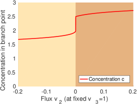
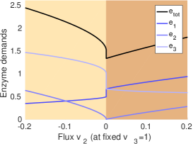
With predefined flux directions and a predefined benefit, our flux profiles are confined to a B-polytope, and we already know that enzymatic flux cost functions are concave on such polytopes. But what happens on the polytope boundaries, where two polytopes touch and fluxes change their directions? An example is shown in Figure 4 (c). Along the polytope boundary, the flux cost is well-defined (to see this, we just have to remove the inactive reactions and study the flux cost function in the remaining subnetwork). But as we cross the boundary, the flux cost function is discontinuous (see Figure 4): there is a jump in the enzyme and metabolite concentrations, and therefore in the flux cost (for an explanation, see SI Figure 8). The boundary always belongs to the polytope with the lower cost. Since flux cost functions are concave within B-polytopes and show jumps on the polytope boundaries, they favour sparse flux profiles, in which many fluxes vanish. For instance, in Figure 4 (e), the flux cost (black line) decreases towards the polytope boundary from both sides, favouring a flux $v_{2}=0$. This effect resembles an L1-regularisation and justifies the sum of absolute fluxes as an approximative cost function (a function with the same property, showing kinks where fluxes are zero).

Box 3: Screening of metabolic states to obtain states with optimal flux profiles
Feasible flux profiles Metabolic states (characterised by enzyme levels, metabolite concentrations, and fluxes) are feasible if they satisfy all constraints defined in a model (e.g. stationarity, rate laws, positive concentrations, and cocentration bounds). The set ${\mathcal{K}}$ of feasible states $({\bf v},{\bf c},{\bf e})$ can be constructed systematically [23]. Each such state can be obtained by choosing a feasible flux pattern (describing the flux directions), then choosing flux and metabolite profiles consistent with this flux pattern, and finally computing the required enzyme levels. Given a flux pattern, feasible flux profiles and metabolite profiles can be found separately by linear programming. For each combination $({\bf v},{\bf c})$, the enzyme levels $e_{l}$ are easily obtained from the rate laws. The difficult task is to find the flux pattern in the first place, allowing for all constraints on fluxes and metabolite concentrations to be respected later on! Importantly, if we consider models with thermodynamically consistent rate laws [22], the feasible choices of ${\bf v}$ and ${\bf c}$ depend only on thermodynamics, and rate laws and the enzyme levels do not play role at this point! We can find flux templates, fluxes and metabolite levels exclusively based on constraints on fluxes and metabolite levels, on the thermodynamic relationships between them. Screening states of a kinetic model Theoretically, metabolic states can be screened as shown on the left. First, we enumerate all feasible flux patterns (i.e. flux signs vectors of). Flux patterns may be infeasible for thermodynamic reasons or because they do not allow for a steady state (i.e. the corresponding orthants in flux space are outisde the hyperplane of stationary flux profiles). For each feasible flux pattern, we construct the corresponding flux and metabolite polytopes, and then screen the two polytopes to obtain all possible flux profiles ${\bf v}$ and metabolite profiles ${\bf c}$. Each combination (${\bf v},{\bf c}$) defines a feasible state, and the corresponding enzyme profile $\mathbf{e}$ is easy to compute. We obtain all possible steady states $({\bf v},{\bf c},\mathbf{e})$. To discard unstable states, each state must be checked by inspecting its Jacobian matrix. The screening allows us to parametrise all metabolic states of a kinetic model by choices of ${\bf v}$ and ${\bf c}$. It shows that the collection of feasible flux polytopes represents all feasible steady states of the model, projected to flux space. Computing the (minimal) enzymatic cost of a flux profile Our screening can be used to find optimal states, e.g. states with a maximal flux benefit per enzyme cost. Metabolic states $({\bf v},{\bf c},{\bf e})$ are scored by flux benefit $b({\bf v})$ (a linear function of fluxes), metabolite cost $g({\bf m})$ (a convex function of logarithmic metabolite levels), and enzyme cost $h(\mathbf{e})$ (a linear function of enzyme levels). We already saw that enzyme and metabolite costs can be written as an effective flux cost $a^{\rm kin}({\bf v})=h(\mathbf{e}({\bf v}))+g({\bf m}({\bf v}))$. To find an optimal flux profile ${\bf v}$ and its associated metabolite profile ${\bf c}$, we define a flux pattern and a flux benefit and minimise enzyme cost across all possible states $({\bf v},{\bf c})$. We can do this in two ways. First, we can screen the flux profiles (scaled to a fixed benefit), find the optimal metabolite profile by ECM, and choose the flux profile with the lowest metabolite-optimised cost. Second, instead, we can screen the metabolite profiles, optimise the flux profile for each of them (with a fixed benefit – which is a linear FCM problem), and choose the metabolite profile with the lowest flux-optimised cost.
Flux cost minimisation with a predefined flux pattern To compute the enzymatic or kinetic cost of a flux profile, we need to find the metabolite profile that realises these fluxes at a minimal enzymatic or kinetic cost. The M-polytope is defined by flux pattern, equilibrium constants, concentration ranges, and external metabolite concentrations. Given our flux profile ${\bf v}$, each metabolite profile ${\bf m}$ on the M-polytope defines an enzyme profile $\mathbf{e}$ (via the enzyme demand function) and therefore a cost. We minimise the cost with respect to ${\bf m}$ and assign the resulting minimal cost to the flux profile as a flux cost function $a^{\rm enz}({\bf v})$ or a kinetic flux cost $a^{\rm kin}({\bf v})$.

3 Flux cost minimisation and flux benefit maximisation

3.1 Flux cost minimisation as a nonlinear FBA with minimal fluxes

If a cell is able to produce biomass (or some other important product) at a low enzyme demand, then protein can be reallocated to other cell functions (e.g. ribosomal proteins). This allows cells to grow faster or to perform extra functions while maintaining its growth rate. Following this logic, cells should strive for enzyme-efficient flux profiles, i.e. flux profiles that provide a given benefit at a minimal enzyme cost. In Enzymatic Flux Cost Minimisation [7], such flux profiles are computed by minimising the enzymatic flux cost $a^{\rm enz}({\bf v})$ at a fixed flux benefit $b({\bf v})=b$ and with given (thermodynamically feasible) flux directions. Flux cost minimisation is a “layered” procedure, with an outer optimisation in flux space and, for each flux profile, an inner optimisation in metabolite space. Aside from cost functions $a^{\rm enz}({\bf v})$ and $a^{\rm kin}({\bf v})$ derived from kinetic models, we may use cost functions defined ad hoc; in any case, flux costs must increase with the fluxes (i.e. $a_{v_{l}}\,v_{l}>0$ for all $v_{l}\neq 0$). This approach works for any plausible flux cost functions, and we obtain a generalised, nonlinear version of minimal-flux FBA: we define a flux benefit $b({\bf v})=b^{\prime}$ and minimise a general flux cost $a({\bf v})$ on the resulting B-polytope. If the flux directions are unknown, we may enumerate all feasible flux patterns (at least theoretically), compute the optimal flux profile for each of them, and choose the best flux profile.

§§§ FCM with enzymatic flux cost functions has some convenient mathematical properties. If the flux directions are given and no flux bounds are imposed, scaling the flux profile as a whole leads to a proportional scaling of flux cost and flux benefit. The cost/benefit ratio yields the scaled flux cost $\hat{a}_{(b)}({\bf v})=a({\bf v})/b({\bf v})$, which is independent of a scaling of ${\bf v}$ and corresponds to the flux cost $a_{(b=1)}({\bf v})$ on the standard B-polytope (defined by $b({\bf v})=1$). In the absence of flux bounds, we can do all our calculations on this B-polytope and compute flux costs on other B-polytopes by simple scaling (see Figure 3). Within our B-polytope, we can directly compare flux profiles (with different active pathways) by their costs. Comparing flux modes at a fixed benefit also works between separate models, e.g. models of different pathways that produce ATP. Also in this case, we can compare flux profiles at a fixed flux benefit (or at a unit benefit, that is, by their cost per benefit). Aside from comparing alternative pathways, there is another reason to run FCM on a B-polytope (and not on the F-cone): on the F-cone, an enzymatic flux cost function will not be stricly concave (because flux cost scales proportionally with the flux profile), whereas on the B-polytope it can be strictly concave.

3.2 Cost-optimal flux profiles are polytope vertices

In FCM, we impose a flux pattern and a flux benefit $b$ and search for flux profiles with this benefit and a minimal cost. Thus, mathematically, we minimise a flux cost function $a({\bf v})$ on a B-polytope. Since the cost function is concave on the polytope, at least one minimum point must be a polytope vertex and at least one polytope vertex must be a minimum point (proof in section B.4). If our cost function is strictly concave, then all minimum points must be polytope vertices. This confirms what we noted before: flux profiles with a minimal enzyme cost favours tend to be sparse.

We can further relate this to Elementary Flux Modes (EFM). Originally, EFMs were introduced to describe meaningful minimal routes in metabolic networks [26, 27]. It was later shown [11, 12] that they also play a role as enzyme-optimal flux profiles in two types of metabolic optimality problems , flux maximisation at a limited total enzyme level; maximisation of enzyme-specific flux. Hence, EFMs are not only a theoretical tool, but have biological relevance: there is always an EFM that provides an equal or higher enzyme efficiency than any non-elementary flux profile. Here we confirmed this result, but for polytope vertices (instead of EFMs). We saw that optimal flux profiles – aside from exceptional cases – are polytope vertices, and in models without flux constraints, these polytope vertices are elementary modes. In models with flux bounds, these extra constraints may cut off polytope vertices (see Figure 7) and create new, non-elementary vertices that are candidates for optimal flux profiles. We come back to this point below.

3.3 Calculation of optimal flux profiles

A flux profile is optimal if it is the one (or one) with the lowest cost on the flux polytope (for a global optimum) or within a small region around the profile (for a local optimum). We can check local optimality by applying the KKT conditions. But there is also a simpler criterion (“Manu’a criterion”): A pair $({\bf v},{\bf c})$of a flux profile ${\bf v}$ and a metabolite profile ${\bf c}$ are locally optimal if (and only if) ${\bf v}$ and ${\bf c}$ favour each other, i.e. ${\bf v}$ is locally optimal given ${\bf c}$ and ${\bf c}$ is locally optimal given ${\bf v}$ (Proposition 4 in SI, proof in SI section E.7). This criterion can be used to test if a flux profile ${\bf v}$ is (locally) optimal: we first compute its favoured metabolite profile ${\bf c}$ (by ECM); then, we compute the favoured flux profile of ${\bf c}$ (by linear FCM) and check whether we reobtain our original flux profile. A variant of this algorithm can be used to generate locally optimal flux profiles: starting from an initial, non-optimal flux profile, we iteratively compute optimal metabolite profiles and optimal flux profiles until convergence (“Manu’a algorithm”, see SI section B.5). The algorithm converges because the cost decreases (or remains constant) in every step (due to biconvexity) and because there is only a finite set of potentially optimal flux profiles (the vertex points). In models without any flux bounds (except for a given flux benefit), optimal flux profiles must be EFMs (or at least one of them must be an EFM). Moreover, if the flux cost function is strictly concave, then any locally optimal flux profile must be an EFM. In theory, finding a global optimum is straightforward: we enumerate all EFMs (with any feasible flux directions) and choose the one with the lowest cost [7]. In practice, the number of EFM may be large and enumerating them may be impossible.

How can optimal flux profiles be predicted in practice? Metabolic states can be optimised by a screening of flux profiles (Box 3). A given flux template and a predefined numerical flux benefit defines a B-polytope; with a concave flux cost function, we can find the optimal flux profile by enumerating all polytope vertices and choosing the one with the lowest cost. Along with the optimal fluxes, we obtain the optimal enzyme and metabolite profiles. Enumerating and testing all polytope vertices may be numerically expensive. Instead of screening them all, we may directly search for a local optimum, either by a greedy search over polytope vertices (e.g. using a simplex algorithm) or by the Manu’a algorithm above. However, to be sure to find the global optimum all polytope vertices need to be screened. By repeating this procedure for different model parameters (e.g. screening kinetic constants or external metabolite concentrations), we can assess their effects on optimal states. The resulting Monod curves and phase diagrams show which metabolic pathways should be used depending on external conditions and enzyme parameters [7].

Until here we assumed that all flux directions were predefined. What if the flux directions themselves are to be optimised? In this case, we need to screen all possible B-polytopes, each representing one possible pattern of flux directions. But this can be simplified. To find the optimal fluxes, we can forget about B-polytopes and simply enumerate all thermodynamically feasible EFMs as well as all feasible non-EFM vertices (in models with flux bounds), and evaluate the flux cost for all these flux profiles. Once the optimal flux profile is known (for the predefined external metabolite concentrations), we also know the best flux pattern and the globally optimal state of our kinetic model.

3.4 Flux optimsiation with extra constraints can lead to non-elementary flux modes

In a basic version of FCM, fluxes must be stationarity and must respect given flux directions, but no other flux bounds. The constraints define a flux cone whose edges are elementary flux modes. If we predefine the flux benefit, the cone is cut by a hpyerplane and reduced to a polytope with corners given by vectors along EFMs. Hence, since FCM (with concave flux cost functions) predicts optimal fluxes to be polytope corners, and since polytope corners are EFMs, optimal flux modes must be EFMs! But what if there are additional bounds on individual fluxes or on linear combinations of fluxes (as proxies for enzyme abundance)? As shown in Figure 7, such constraints can cut off parts of the polytope and create new polytope vertices. The new non-elementary vertices are (somewhat confusingly) called “elementary flux vectors” (EFV) [28]. By adding more flux constraints, we may obtain more vertices, each representing a convex combination of EFMs (with a maximal number of $n$ EFMs if $n$ is the number of constraints). The convex set spanned by these EFVs is still a polytope, but not one that is spanned by EFMs. All its vertices are potential solutions of FCM problems.

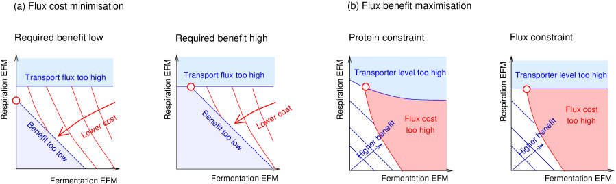
We saw that the optimal flux profiles are B-polytope vertices. In models without other flux bounds, these vertices are elementary modes, but in models with flux bounds, non-elementary vertices can appear. Let us see an example. In cell metabolism, ATP is typically generated by glycolysis, whose product pyruvate is either exported (overflow metabolism) or used to produce more ATP (via respiration). In our model in Figure 1, the (high-yield) respiration and (low-yield) overflow strategies are EFMs, suggesting that one of them should be optimal linear combinations of them should be worse. In reality, some cells may ferment and respire simultaneously (e.g. overflow metabolism in bacteria, the Crabtree effect in yeast, and the Warburg effect in cancer cells). Moreover, in E. coli chemostat cultures the ratio between the two fluxes (or the ratio of glucose uptake and acetate overflow) varies gradually with the growth rate. This cannot be explained by a switch between EFMs, but enatils at least a varying combination of EFMs. So what is wrong with our model?

In FBA or resource allocation models, non-EFMs may occur as polytope vertices due to flux constraints describing limited total protein levels, limited uptake rates, or limited membrane space [29]. For example, non-EFM acetate overflow in E. coli has been predicted by assuming a bound on glucose uptake efficiency which limits respiration, whenever glucose uptake is high, through competition for protein resources [30]. A similar possible constraint is the competition for bacterial membrane space (“real estate”) between glucose transporters and the respiratory chain in bacteria [31]. In FCM, similar constraints can be applied to predict non-elementary flux modes.

The existence of non-elementary polytope vertices may explain observed flux distributions like in the Crabtree effect. Respiro-fermentation (instead of fermentation alone) can be predicted by putting a bound on the respiration flux as shown in Figure 1 (e.g. representing space limitations for respiratory chain complexes in mitochondrial membranes).

Figure 5: Bounds on fluxes and enzyme levels can lead to non-elementary flux solutions. (a) Flux cost minimisation with a lower bound on flux benefit (schematic example). The axes correspond to fluxes in EFM “respiration” or EFM “fermentation” and are scaled to units of flux benefit (e.g. ATP production rate), the benefit constraint line is a decreasing 45 degrees diagonal. Left: The optimum point (red circle) represents pure respiration. Right: The same problem with a tighter bound on the benefit. The new optimal flux profile (red circle) is a combination of the two EFMs, describing respiro-fermentation (compare Figure 1). (b) Flux benefit maximisation (FBM). Left: Protein constraint (in this case, an upper bound on the glucose transporter). The bound is curved and concave (as a contour line of a concave (protein cost) function). Like in (b), the optimum point can be a vertex of the feasible region. Right: A linear flux constraint approximates the protein constraint: a bound on the glucose transport flux (mimicking the bound on the transporter level) is easy to handle computationally.

The idea that optimal flows must be EFMs has led to advances in metabolic modelling. However, how useful is it in practice?

1. We saw that optimal solutions, as polytope vertices, need not be EFMs but can also be combinations of EFM. First, it depends on model assumptions, most notably on the absence of additional flux constraints. In respiro-fermentation, occurring in the Crabtree effect in yeast and in the Warburg effect in cancer cells, overflow metabolism takes place on top of (and not instead of) respiration. If a model describes overflow and respiration as EFMs (like the model in Figure 1), a non-elementary respiro-fermentation mode can still be explained by a bound on the respiration flux.

2. May not hold in models with non-enzymatic reactions

3. Second, the claim that “optimal flux profiles must be EFMs” may raise some epistemological problems. The reason is that EFMs are defined only within a model, with reference to a metabolic network structure and a choice of external metabolites. Howeverm the “complete metabolic network” of cells (which would contain all non-enzymatic reactions or unknown side reactions of enzymes) is hardly known and not even well-defined. Also, what counts as “external metabolites” is a matter of choice: cofactors can be treated as strongly buffered (and therefore external), or as variable (and therefore “internal”). All these choices make the set of EFMs model-dependent, and so our statement that “optimal flux profiles must be EFMs” is in fact not a statement about cells, but about cell models.

4. Finally, the cost difference between an optimal elementary metabolic state and some other non-optimal states may be so small that this latter non-EFM solution may be realised by cells either because of other advantages, or because they are simply not costly enough to be suppressed.

3.5 Flux benefit maximisation

If flux profiles reflect a trade-off betwork (enzyme) cost and (production) benefit, how can we describe these trade-offs mathematically? One possibility is to maximise the benefit/cost ratio (or “biomass/enzyme productivity”). Like in a single reaction, we may expect that flux profiles should be enzyme-efficient, showing a high biomass production per enzyme invested. As we will see, higher metabolic efficiencies allow for a higher growth rates [6]. However, instead of minimising the ratio directly, we may also minimise the cost at a fixed benefit or maximise the benefit at a fixed cost (as in mcFBA).

FCM can be seen as a nonlinear version of FBA with minimal fluxes, a version in which enzyme efficiencies are not fixed, but are optimised along with the fluxes. Similarly, we can imagine a nonlinear form of FBA with molecular crowding, in which we maximise a flux benefit while constraining the flux cost. This method is called Flux Benefit Maximisation (FBM). Again, the flux cost can be a proxy for the amount of catalysing enzymes: using enzyme cost as a constraint (and not as an objective) allows us to implement density constraints for multiple cell compartments.

In FCM and FBM problems, flux constraints can represent enzyme constraints. In a maximisation of flux benefit, bounds on fluxes or on linear combinations of fluxes yield plane constraint surfaces that cut off parts of the polytope (see Figure 5 (b)). Enzyme constraints, instead, would yield curved constraint surfaces (defined by non-concave enzyme cost functions). Just like constraints on flux cost, these constraints can cut off vertices and give rise to non-elementary vertices, leading to “mixed strategies” such as respirofermentation. If we replace an enzymatic cost function $a^{\rm enz}$ (used to define a bound in flux space) by a linear approximation (see section 3.6), we obtain a linear flux constraint on the flux polytope as in FBA with molecular crowding. Thus, FBM with linearised protein constraints effectivly resembles FBA with molecular crowding, but with kinetics-dependent transporter efficiencies like in satFBA.

On a fast timescale, cells cannot adjust their enzyme levels, but may still regulate their fluxes, for example, by enzyme phosphorylation. Let us consider a variant of FBM that describes this. The cell’s strategy is to have enzyme overcapacities that can quickly be mobilised to adapt to changes in the environment. The search for the right enzyme levels for such a preemptive expression can be formulated as an optimality problem: cells need to choose an enzyme profile that will enable them to realise a number of predefined useful flux profiles by inhibiting some of the enzymes. Finding the cheapest enzyme profile that does this is a convex optimality problem (see [10], Supplementary information). But once the enzyme profile s fixed (and the enzyme cost spent), which fluxes (i.e. what enzyme inhibition pattern) should the cell choose in a given environment? The problem resembles classical FBA (with bounds on individual fluxes, but now the bounds are on enzyme activities). Assuming that enzymes can be inhibited, each enzyme activity can vary between 0 and our predefined enzyme amount. If the aim in this is to maximise flux benefit under these constraints, we obtain a variant of the FBM problem (see SI C.2).

3.6 Linear flux cost functions

In flux analysis, enzyme efficiencies play a key role: they provide a linear conversion formula between fluxes and enzyme levels, needed to define density constraints (in FBA with molecular crowding) or linear flux cost functions (in minimal-flux FBA). For a linear conversion, it is assumed that the catalytic rates are fixed and given, as if the metabolite concentrations were constant. In FCM, in contrast, we acknowledge that enzyme efficiencies can vary and are co-optimised with the fluxes. The resulting models are more realistic, but the flux cost functions become nonlinear, resulting from an optimality problem on the M-polytope, and are harder to optimise than the linear cost functions in FBA. This increases the numerical effort: in FCM, we need to solve an optimality problem for each vertex of the B-polytope. Also in flux sampling, e.g. to study cell populations with Boltzmann-distributed flux profiles (see section 4.2) we need to assess many flux profiles and compute their enzymatic costs. In this case, to speed up the calculations we may replace the enzymatic flux cost by linear or quadratic approximations (see SI section A.4). To obtain a linear approximation, we simply linearise our cost function around a “prototype” flux profile. In practice, we just compute the optimal catalytic rates $k_{l}=v_{l}/e_{l}$ in this state and use them for all other flux profiles. The flux cost weights $a_{v_{l}}=h_{e_{l}}/k_{l}$, obtained from our prototype fluxes, can be used in FBA with minimal fluxes or with molecular crowding. By deriving them from kinetic models, we see what the cost weights actually mean and obtain a justification for FBA. By using several reference states instead of one, we obtain ranges or quadratic approximations of the flux cost. Given the flux cost and flux cost gradients for two flux profiles, the cost function on the interpolation line can be bounded by linear functions (see appendix A.2). Finally, we may choose several flux profiles in different regions of the flux polytope. Each of these prototype profiles will come with a vector of enzyme efficiencies, and by interpolating these enzyme efficiencies on the flux polytope, we obtain a (non-convex) quadratic flux cost function.

We saw that flux cost weights for FBA can be derived from enzymatic flux cost functions (e.g., by evaluating the optimal enzyme efficiencies for some reference flux profile by ECM). By doing so, we can link cost weights directly to the parameters of underlying kinetic models, thus linking FBA to enzyme kinetics. Compared to a nonlinear FCM problem, FBA with minimal fluxes is easy to solve. At the same time, it captures two main features of FCM: since linear cost functions are concave, optimal flux profiles will be polytope vertices, just like in FCM! . and that, therefore, the flux solution jumps between discrete, qualitatively different flux profiles as model parameters are changing. However, there is a downside: linear flux cost functions chosen ad hoc miss some important details, e.g. the fact that flux cost functions are curved, the possible metabolite cost terms, and the way flux costs wil vary with external metabolite concentrations.

A main problem with linear flux cost functions is that the cost weights are chosen ad hoc, and that their dependence on enzyme kinetics, metabolite concentrations, and environmental conditions remains unclear. Methods such as FBA with molecular crowding [3] use a flux burden vector ${\bf a}_{\rm v}=h_{\rm e}/k_{\rm cat}$. It reflects $k_{\rm cat}$ values and enzyme cost weights $h_{e_{l}}$ (e.g. enzyme sizes), but ignore the effects of metabolite concentrations. This underestimates the flux cost and hides its dependence on parameters such as external metabolite concentrations. In some FBA methods, such dependencies have been considered for single reactions, e.g. by assuming a transporter kinetics $v(c)=u\,\frac{k_{\rm cat}\,c}{K_{\rm M}+c}$ and writing the burden of the transport reaction as $a_{v}=h_{\rm e}\frac{u}{v(c)}=\frac{h_{\rm e}}{k_{\rm cat}}(1+\frac{K_{\rm M}}{c})$ of the external nutrient concentration. This flux cost function depends on extracellular concentrations: the lower the concentration, the higher the transporter’s effective price. However, all metabolite concentrations inside the cell are assumed to be constant, which is unrealistic. This is the dilemma: a realistic expression for flux cost weights will depend on all metabolite concentrations! An external drop in nutrient concentration, will not only increase the transporter demand (first-order effect); instead, also all other enzyme leves are readjusted, resulting in a slightly higher enzyme demand in many of the reactions. This means that all flux cost weights will change, and this change depends on all model details, including possibly metabolite cost terms! If we linearise an enzymatic (or kinetic) flux cost function, how can we predict the resulting flux cost weights depending on all these factors? FCM provides a solution: by deriving flux cost weights from linearised enzymetic costs, it shows how these weights depend on enzyme efficiencies and therefore on model parameters and external metabolite concentrations. These efficiencies for a “prototype” state. In using a linear flux cost function, we presume that the same efficiencies also hold for other flux profiles. The resulting flux cost weights depend on all model details, including $K_{\rm M}$ values, the growth medium and bounds on metabolite levels. Any changes in these parameters will change the flux cost weights. As an example, consider a respiring cell. If the oxygen level (a model parameter) decreases, this alters the M-polytope and the cost function $g^{\rm enz}(\ln{\bf c})$ on this polytope, so also the enzymatic flux cost function $a^{\rm enz}({\bf v})$ will change. A lower oxygen level leads to a lower driving force in oxidative phosphorylation, which increases the enzyme demand. If we linearise $a^{\rm enz}({\bf v})$ to define cost weights for FBA, the resulting cost weights will depend on the oxygen level, and FCM describes this dependence based on kinetic models. Of course, this holds not only for oxygen levels, but for any other model parameters. In summary, FCM assumes the same logic as satFBA (low substrate levels leads to higher enzyme demands), but applies it to all reactions and assumes (optimality-based) metabolite changes inside the model. The resulting enzyme efficiencies (and flux cost weights) are more realistic (and better justified theoretically) than the usage of $k_{\rm cat}$ values or empirical apparent $k_{\rm cat}$ values.

4 Protein demand and cell growth rate

4.1 Cell growth rate as a function in flux space

In metabolic models with a biomass reaction, the overall metabolic efficiency can be described by biomass/enzyme productivity, that is, the biomass production rate divided by the total concentration of metabolic enzyme . Its reciprocal value, the metabolic enzyme concentration per biomass production, is also called biomass-specific enzyme demand. Metabolic efficiency also has an effect on resource allocation: if the growth conditions are good (e.g., good carbon sources or high substrate levels) and allow for a given metabolic production at a lower amount of enzyme, cells can shift of protein investments from metabolic enzymes towards ribosomes, increase their metabolic fluxes and translation rates simultaneously, and therefore grow faster. The biomass-specific enzyme cost $\hat{a}^{\rm enz}$ can be converted into a cell growth rate $\lambda$ by a cost-growth conversion function $\lambda(\hat{a}^{\rm enz})$. This function allows us to describe cell growth rate as a function on the flux polytope! A formula (with a monotonically decreasing function) can be obtained from simple protein allocation models [6]; if we use it, we conclude that FCM solutions also maximise cell growth. Since $\lambda(\hat{a}^{\rm enz})$ is a decreasing function, maximal cell growth requires a minimal biomass-specific enzyme demand, which means that growth-maximising flux profiles can be found by FCM.

To make the link between enzyme efficiencies and cell growth, let us have a look at resource allocation models for cells. In these models, metabolic efficiency and choices of metabolic strategies play a main role. In whole-cell models, metabolism and protein synthesis (or, generally, macromolecular processes) depend on each other: metabolism provides precursors for protein synthesis, while enzymes catalyse metabolic reactions. The coupled system needs to produce all cell components (to duplicate the cell, or in other words, to keep all compounds at constant concentrations despite their dilution). Finally, a density constraint (e.g. an upper bound on the total volume occupied by protein) makes proteins compete for space and, indirectly, for other resources. In a simple resource allocation model, there are just two types of proteins, metabolic enzymes and the translation machinery, which share a limited protein budget. To maximise growth, this budget needs to be optimally shared between the two functions, finding a best compromise between efficient precursor and protein production. In FBA, cell growth is often associated with the biomass reaction rate, setting $\lambda=v_{\rm BM}/c_{\rm BM}$. While this is correct in principle, it ignores two important facts: first, the predicted biomass rate $v_{\rm BM}$ depends on the uptake fluxes (which are variable and generally unknown), and putting fixed bounds on the uptake rates will not give realistic results. This problems is partially solved by FBA with molecular crowding. Second, FBA ignores variable resource allocation between metabolism and protein synthesis (or any cell processes outside metabolism). This problem is solved by CAFBA. . In FCM, like in FBA, we focus on metabolism and ignore protein synthesis. The resulting biomass/enzyme productivity can be related to cell growth in two steps : given a kinetic model and growth conditions (external compound concentrations), we can translate flux profiles into enzyme efficiencies, and compute an optimal biomass production per total metabolic enzyme. We then convert the biomass/enzyme productivity into a growth rate, either by applying an empirical formula (from growth-rate dependent proteomics data) or by using a simple resource allocation cell model. Since the metabolic enzyme demand depends on biomass/enzyme productivity (e.g. biomass production rate per total enzyme investment), the optimal resource allocation and growth rate (in protein partitioning models or RBA) are directly linked to the question of metabolic efficiency, i.e. the metabolic production per enzyme amount (which can be computed by FCM).

How can a cost-growth formula $\lambda(\hat{a}^{\rm enz})$ be derived? We assume a partitioning of protein resources between enzymes and ribosomes, as used to explain bacterial growth laws [6, 7]. The original minimal proteome partitioning cell model from [6] has been extended in various ways [30, 32, 33]. In the basic model, cell growth is proportional to protein production, which consists of two steps, $\stackrel{{\scriptstyle 1}}{{\rightarrow}}\mbox{Precursors}\stackrel{{\scriptstyle 2}}{{\rightarrow}}\mbox{Protein}$, catalysed by metabolic enzymes (1) and ribosomes (2). We assume that protein precursors are mass-balanced, reaction rates are proportional to the catalysing proteins, and the protein budget for enzymes and ribosomes is fixed. By putting all this together, we obtain a formula that converts the enzyme/biomass demand $\hat{a}^{\rm enz}$ into cell growth,

$$\lambda(\hat{a}^{\rm enz})=\lambda^{\rm max}\,\frac{a_{0}}{a_{0}+\hat{a}^{\rm enz}}.$$ (9)

The formula contains two parameters: a maximal growth rate $\lambda^{\rm max}$ and an effective parameter $a_{0}$, denoting the specific enzyme cost that leads to a half-maximal growth rate. We used the cost-growth function (9) to predict cell growth rates in [7]. By defining the biomass/enzyme productivity $k_{\rm BM}=1/\hat{a}^{\rm enz}$, we obtain the efficiency-growth function

$$\lambda(k_{\rm BM})=\lambda^{\rm max}\,\frac{k_{\rm BM}}{k_{\rm BM}+k_{0}},$$ (10)

where the parameter $k_{0}=1/a_{0}$ denotes the biomass/enzyme productivity that would lead to half-maximal growth. If $k_{\rm BM}\ll k_{0}$, as we found for E. coli [7], Eq. (10) can be approximated by a simple proportionality $\lambda\sim k_{\rm BM}$. We obtain the same linear formula by postulating that metabolic enzymes occupy a fixed fraction of the biomass, indpendent of the growth rate. Then we write $\lambda=\frac{v_{\rm BM}}{c_{\rm BM}}=\frac{v_{\rm BM}}{\hat{a}^{\rm enz}}\frac{\hat{a}^{\rm enz}}{c_{\rm BM}}$: the first fraction is our biomass production efficiency $k_{\rm BM}$, and the second fraction (the protein budget for metabolic enzymes, per biomass) is the (supposed) constant biomass fraction.

Using the enzyme/biomass demand $\hat{a^{\rm enz}}({\bf v})$ and the conversion formula (9), the growth rate can be written as a function $\lambda({\bf v})$ on the flux polytope. By maximising this function, we obtain the flux profile (and the corresponding metabolite and enzyme profiles) that allows for maximal cell growth. Since the conversion function (9) is monotonically decreasing, we can simply obtain the same state by FCM. Again, the flux profiles that maximise growth are polytope vertices.

4.2 Cell populations described by probability distributions on the flux polytope

In a cell population, cells will show different flux profiles. If we describe cells by points in flux space, the population forms a point cloud, which may be described by a probability distribution. If the probability density on the flux polytope is known, we can infer the average flux profile and the distributions and correlations of different reaction fluxes. To obtain such a distribution, we can consider a simple model of cell populations in which fast-growing cells also reproduce faster and are more abundant in the population. We describe each cell by a point on the B-polytope, that is, a flux profile ${\bf v}$ with growth rate $\lambda({\bf v})$. Inspired by statistical physics, we define a simple probability density function: we define a Boltzmann distribution with the inverse growth rate as a “negative energy” function and obtain the probability density

$$p({\bf v})\sim\mbox{\rm e}^{(\lambda({\bf v})-\lambda_{d})/\xi},$$ (11)

where $\lambda$ is the cell growth rate and $\xi$ describes the strictness of selection and $\lambda_{d}$ is chosen to normalise $p$ to a total probability of 1. The Boltzmann formula with flux cost as an energy function can derived from a simple population model (SI D). In the model, cells grow for a fixed time interval $\tau=1/\xi$ with its growth rate $\lambda({\bf v})$, then each cell switches randomly to a new flux distribution (drawn from a uniform distribution on the flux polytope) or dies with a death rate $\lambda_{d}$ (identical for all cells and adjusted to maintain a constant population size). This stochastic process converges to an invariant distribution, the Boltzmann distribution (11). Instead of the Boltzmann distribution (11), we can also use another possible probability distribution with the density

$$p({\bf v})\sim\frac{1}{1-(\lambda({\bf v})-\lambda_{d})/\xi}.$$ (12)

To derive this formula, we assume that cells can switch their flux state in any moment with a characteristic rate $\xi=1/\tau$, where $\tau<1/\lambda$ is required (see appendix D). Mathematically, the distribution (12) resembles the Fermi-Dirac and Bose-Einstein distributions in quantum statistics (see appendix E.12).

The probability densities Eq. (11) or (12) tell us about average fluxes, flux variability, and flux correlations in a cell population. They also define, implicitly, probability distributions for the (ECM-optimised) metabolite and enzyme levels.There is no closed formula for all these quantities, but we can use Monte Carlo sampling: by sampling flux profiles and recording the corresponding metabolite and enzyme profiles, we obtain an ensemble of cell states. To characterise this ensemble, we can use concepts from statistical mechanics, such as the partition function, entropy, mutual information, and a quantity analogous to the free energy, an effective population growth rate that accounts for the dispersion of cell states. Interestingly, our cell population models are linked to thermodynamics in two ways: on the one hand, we use tools from statistical mechanics for describing cell populations; on the other hand, within our metabolic models themselves, thermodynamics determines flux directions, shapes flux and metabolite profiles, appears in rate laws and enzyme demand functions, and thereby shapes flux cost function. When working with probability distributions, defined as in [34] or here, an open problem is the choice of a metric or “density of states”.

5 Discussion

We saw how enzymatic flux costs $a^{\rm enz}({\bf v})$ and kinetic flux costs $a^{\rm kin}({\bf v})$, together with optimal metabolite concentrations ${\bf c}({\bf v})$ and enzyme levels $\mathbf{e}({\bf v})$, can be derived from kinetic models. While $a^{\rm enz}({\bf v})$ captures enzyme cost only, $a^{\rm kin}({\bf v})$ considers both enzyme and metabolite costs. The costs may represent, for example, occupied space or invested carbon or energy. Importantly, these concentration profiles are not the only ones that can realise the fluxes ${\bf v}$, but they are the ones that can do that at a minimal cost. Our flux cost functions depend on rate laws, kinetic constants, and external metabolite levels. Although they may be hard to compute, they have some simple general properties. A proportional scaling of fluxes and enzyme levels leaves metabolite levels (and therefore enzyme efficiencies) unchanged. As a consequence, the enzymatic flux cost scales proportionally with the flux profile and we obtain simple sum rules for its derivatives. Moreover, enzymatic flux cost functions are concave (and often strictly concave). When two flux profiles are added or interpolated, they need to “negotiate” a common optimal metabolite profile; this leads to a compromise cost. If two flux profiles favour the same metabolite profile, there is no compromise cost between them, the flux costs are additive and the flux cost function between them is linear. Otherwise, the flux cost function is strictly concave, so there is a compromise cost, and any optimal flux profiles must be vertices of the flux polytope. This confirms the idea that “optimal flux distributions must be EFMs” [12, 11] and generalises it to models with flux constraints.

The flux cost functions defined by kinetic models also tell us about some general features a flux cost function should have: it should increase with the fluxes, be concave on each F-polytope, but discontinuuous between F-polytopes. The resulting flux distributions will be sparse, located on F-polytope boundaries rather than in its interior. This excludes heuristic flux cost functions like the sum of squared fluxes, which are convex with an optimum inside a B-polytope. Of course, such functions may be used for other reasons (e.g. for obtaining a simple unique solution based on a principle of minimal information) as in geometric FBA, stating that alternative pathways fluxes should be used simultaneously unless data are telling us otherwise. But as proxies for actual enzyme cost, such functions are poorly justified.

Flux cost functions allow us to predict optimal fluxes and growth rates based on metabolite and enzyme costs, kinetic laws, and physiological constraints (e.g. bounds on metabolite levels). By converting metabolite and enzyme costs into flux costs, we can replace the search for optimal states by a simple optimisation of fluxes. In different variants of this optimisation, flux cost and flux benefit are either treated as objectives or as constraints. FCM (a generalised form of FBA with minimal fluxes) minimises flux cost at given flux benefit, FBM (a generalised form of FBA with molecular crowding) maximises flux benefit at a bounded flux cost, while linear-fractional programming optimises the benefit/cost ratio directly. In the absence of flux bounds (in general, weighted sums of absolute fluxes), flux solutions are scalable and we need to impose a scaling (e.g. by fixing the flux benefit) to obtain a specific solution. In contrast, with fluxes being bounded, the absolute scaling of fluxes matters: if a flux hits a bound, the fluxes cannot be further increased by scaling, and the only way to (possibly) increase the flux benefit is by changing the shape of the flux profile. Therefore, if flux constraints are imposed (e.g. a bound on respiration due to limited membrane space), this does not only affect the scaling, but also the shape of optimal flux distributions. Instead of assuming a single objective, we may treat different targets (such as enzyme cost, biomass production, or biomass yield) as separate objectives and describe optimal compromises (e.g. between flux-derived growth rates and yield [7]) as Pareto-optimal points [15, 16]. This approach can be generally used to capture multiple cost and benefit functions.

In flux prediction, fluxes or enzyme levels can be constrained. If enzyme demands are linearly approximated, the two types of bounds play similar roles: assuming constant enzyme efficiencies, enzyme bounds can be written as flux bounds. In molecular crowding FBA and CAFBA, this link between fluxes and enzyme levels is used to formulate resource allocation principles directly for fluxes. However, flux constraints can also be justified in different ways. A constraint on glucose transport flux may reflect a bound on transporter abundance (at a given external glucose level), but also an economical usage of glucose (avoiding unnecessary import fluxes, and unnecessary losses by export fluxes). We saw that flux optimisation under constraints can lead to non-elementary flux distributions. But there are also other reasons for non-elementary fluxes. By adapting their enzyme levels, cells can save enzyme resources; but if enzyme levels are fixed (on a time scale of interest), cells can still optimise their fluxes by changing the enzyme activities (e.g. by protein phosphorylation). Flux optimisation in this case can be formulated as a convex problem, but one that may lead to non-EFMs (see SI C.2).

The flux cost functions in FBA are usually chosen ad hoc: it remains unclear which actual costs they represent, whether they can capture metabolite costs, and how they depend on real biochemical parameters. Enzymatic and kinetic flux costs, in contrast, are related to enzyme efficiencies derived from kinetic models in optimal states. In molecular crowding FBA, CAFBA, and Resource Balance Analysis , these enzyme efficiencies are key model parameters with a a big impact on metabolic strategies. If constant enzyme efficiencies and enzyme prices $\partial h/\partial e$ are assumed, this leads to constant flux burdens to be used as cost weights in linear flux cost functions. Linear flux cost functions are widely used in flux modelling, but often without a good justification: for example, linear relationships between fluxes and enzyme levels are assumed, claiming that enzyme work at their maximal capacity ($k_{\rm cat}$ value) or at a constant capacity (“apparent $k_{\rm cat}$ value”). In reality, the $v/e$ ratios can vary between metabolic states, and knowing these numbers is of utmost importance in FBA. We saw how enzyme efficiencies depend on kinetics, on external conditions, and on the resulting optimal metabolite profile), and that we can predict them by ECM. We also learned that nonlinearities in enzyme cost functions (which we call compromise costs) stem from the fact that different flux profiles favour different metabolite profiles, and thus different catalytic rates. If two flux profiles favour the same metabolite profile, and therefore go with the same enzyme efficiencies, flux costs can be linearly interpolated. The above construction of linear flux costs functions from kinetic models justifies their usage in FBA and shows how the cost weights depend on details of the kinetic model and how they vary between growth conditions.

Flux cost minimisation relies on many simplifying assumptions. What if we abandon some of them? (i) Nonlinear enzyme cost functions. Instead of assuming a linear enzyme cost function, we may assume a nonlinear function $h(\mathbf{e})$. As long as this function is convex, the ECM problem will also be convex. However, some other results may not hold: enzymatic flux cost functions will not scale proportionally with the flux profile and may become non-concave (the proof in SI E.1 does not apply in this case). However, the change from a linear enzyme cost function to a convex one will not change the optimal flux solutions. (ii) Non-enzymatic reactions. Non-enzymatic reactions are hard to handle in FCM (see SI section C.3). Their presence changes the shape of metabolite and flux polytopes and of the enzymatic F-cost function. This can be explored numerically (non-enzymatic reactions may lead to constraints on the M-polytope, which can be handled in ECM), but the optimal solutions may be non-EFMs. (iii) Stabilisation of metabolic states. Unstable metabolic steady states can be stabilised by feedback control, e.g. enzyme inhibition by pathway products. Compared to the same model without inhibition, the enzyme level needs to be higher to yield the same reference flux. Also a simple overexpression of enzymes, which keeps the enzymes far from saturation, can stabilise metabolic states. In models, such extra enzyme investments would add to the enzymatic flux cost and would possibly make it non-concave.

In this paper, we assumed that cells strive for maximal metabolic efficiency, defined as a production flux (or other linear flux objectives) divided by an enzyme (or enzyme plus metabolite) cost. To implement this in models, one may minimise cost at a fixed benefit (in FCM) or maximise benefit at a fixed cost (in FBM). While optimising enzyme efficiency can serve as a useful heuristics, in reality cells do not strictly save enzyme resources or maximise catalytic rates. During a metabolic switch, Lactococcus lactis bacteria [35] inhibit some of their enzymes (thus reducing their efficiency) while they could have saved enzyme costs by repressing enzymes transcriptionally [35]. How can we explain this behaviour? Unnecessary enzymes allow cells to quickly adapt to environmental changes. Enzymes may have also other functions or side benefits (e.g. serving as an amino acid storage). By ignoring these effects, FCM provides a theoretical minimal cost of a flux, and the corresponding maximal growth rate. Even if they are overly simplified, these predictions can be usefule as a null hypothesis for testing other optimality scenarios (e.g. optimality scenarios that include preemptive expression, side objectives for proteins or metabolites, or simply non-optimality) and to compute the difference in enzyme cost.

Appendix A Metabolic flux profiles and flux cost functions

A.1 Metabolic models, metabolic flux profiles, and flux polytopes

Metabolic models We consider metabolic network models with reversible rate laws of the form $v_{l}=e_{l}\,k_{l}({\bf c})$ (where $e_{l}$ denotes enzyme levels). The catalytic rate $k({\bf c})$ of an enzyme $l$ can be factorised into capacity, reversibility, and kinetic terms $k=k_{\rm cat}\cdot\eta^{\rm rev}({\bf c})\cdot\eta^{\rm kin}({\bf c})$ [10]. To model fitness incentives and physiological requirements in a cell, we consider three metabolic targets: $b({\bf v})$ (linear flux benefit function), $g({\bf c})$ (convex metabolite cost function), and $h({\bf e})$ (linear enzyme cost function). Typically, the flux benefit scores the production of valuable compounds or biomass, while the cost terms describe growth disadvantages caused by higher protein or metabolite concentrations. Under simplifying assumptions, the ratio [enzyme cost]/[flux benefit] can be translated into a cell growth rate (see section E.11).

Metabolic flux profiles, scaled flux profiles, and flux modes if a flux distribution ${\bf v}$ is stationary (satisfying the condition ${\bf N}^{\rm int}\,{\bf v}=0$), it is called a metabolic flux profile or, if the absolute scaling is disregarded, a flux mode. An elementary flux mode is a flux mode with a minimal set of active reactions: if one more reaction flux were restricted to zero, the remaining active reactions would not be able to support any stationary flux distribution. Flux modes can be seen as scaled flux profiles. For example, with a “target flux” $v_{r}$ (e.g. biomass production) we can define the scaled flux profile ${\bf v}/v_{r}$ and the scaled flux cost $a^{\rm sc}({\bf v})=a({\bf v})/v_{r}$, i.e. the flux cost per target flux. If a flux profile ${\bf v}$ is multiplied by a factor $\sigma$, the scaled flux profile and the scaled cost remain unchanged.

Flux patterns and conformal flux profiles The sign vector of a flux profile ${\bf v}$ is a vector with elements 1,0, and -1, describing the set of active reaction and flux directions. Such vectors are called flux patterns. A flux profile is conformal with a given flux pattern if all active fluxes match the prescribed signs (zero fluxes are allowed even if signs 1 or -1 are prescribed). A flux profile ${\bf v}$ is said to have (or to be “strictly conformal with”) a given flux pattern if the flux signs exactly match the prescribed signs (in this case, a prescribed sign of 0 means that the flux must vanish). Two flux profiles are called conformal if they are conformal to a common flux pattern, i.e. if all their shared active reactions show the same flux directions. Two flux profiles are strictly conformal if they have exactly the same flux pattern. All these definitions also hold for flux modes instead of metabolic flux profiles.

Feasible flux patterns A metabolic network allows for many flux patterns, but only some of them are physically and physiologically feasible. To be realised with reversible kinetic rate laws, a flux profile must be thermo-physiologically feasible: this means, there must be a choice of metabolite concentrations that respect the physiological concentration ranges defined in the model and that allow the flux profile to be realised under thermodynamic constraints on the flux directions. This requires that the flux profile is loopless. The flux pattern of a thermo-physiologically feasible flux profile is called thermo-physiologically feasible as well. Briefly, a feasible flux pattern is a flux pattern that can be realised by fluxes that are stationary, thermodynamically feasible, and that realise the predefined flux benefit.

Flux polytopes Each flux pattern corresponds to a segment in flux space, i.e. to an orthant or one of its lower-dimensional surfaces. If a segment intersects the subspace of stationary fluxes, the intersection set is called an F-cone (“signed flux polytope”) ${\mathcal{P}}_{\rm F}$. All flux profiles in the interior of an F-cone are strictly conformal. If two flux profiles are conformal, they belong to a common F-cone. If a flux pattern excludes negative fluxes, the F-cone is called a positive flux polytope ${\mathcal{P}}_{\rm P}=\{{\bf v}|{\bf N}\,{\bf v}=0;{\bf v}\geq 0\}$.

Reorienting the reaction directions The flux signs in a model depend on the reaction orientations, i.e. which compounds are treated as substrates or products by definition. This is a matter of convention, and independent of the actual flux directions. Since F-cones can always be converted into P-polytopes (by reorienting the reactions), we can assume (without loss of generality) that fluxes are non-negative.

Benefit-scaled polytope If we restrict an F-cone to flux profiles with a fixed benefit $b({\bf v})=b$, we obtain a B-polytope (“benefit-restricted flux polytope”), which is convex and has one dimension less than the F-cone. A flux pattern is feasible if it corresponds to a segment of flux space that contains a non-empty B-polytope, for the kinetic model, concentration ranges, and flux benefit function in question.

Combined flux profiles The interpolation between two flux profiles ${\bf v}_{\rm A}$ and ${\bf v}_{\rm B}$, with interpolation parameter $0<\sigma<1$, yields a combined flux profile ${\bf v}_{\rm C}=\sigma\,{\bf v}_{\rm A}+[1-\sigma]\,{\bf v}_{\rm B}$; in this combination, the flux profiles ${\bf v}_{\rm A}$ and ${\bf v}_{\rm B}$ are called the basic flux profiles. Combinations of three or more flux profiles are defined accordingly. If several flux profiles belong to one F-cone, their combined flux profiles also belong to this polytope.

Metabolite polytope In a given metabolic model, a flux profile pattern does not only define an F-cone, but also a metabolite polytope (or “M-polytope”) ${\mathcal{P}}_{\rm M}$ for metabolite profiles. It is the set of (natural) log-concentration vectors ${\bf m}=\ln{\bf c}$ that respect the given bounds on individual concentrations and are thermodynamically feasible for the given flux directions.

A.2 Flux cost function and compromise cost

Definition A.1

Flux cost functions We consider a kinetic model with enzyme cost $h({\bf e})$ and metabolite cost $g({\bf m})$ and define the cost functions

$$g^{\rm enz}({\bf m};{\bf v}) = h({\bf e}({\bf m};{\bf v}))\;\,\quad\qquad\qquad\quad\mbox{(Enzymatic metabolite cost)}$$

$$g^{\rm kin}({\bf m};{\bf v}) = h({\bf e}({\bf m};{\bf v}))+g({\bf m})\;\qquad\quad\mbox{(Kinetic metabolite cost)}$$

$$a^{\rm enz}({\bf v}) = \mbox{min}_{\bf m}\,g^{\rm enz}({\bf m};{\bf v})\,\qquad\qquad\mbox{(Enzymatic flux cost)}$$

$$a^{\rm kin}({\bf v}) = \mbox{min}_{\bf m}\,g^{\rm kin}({\bf m};{\bf v})\;\qquad\qquad\mbox{(Kinetic flux cost)},$$ (13)

where the log-metabolite profile ${\bf m}=\ln{\bf c}$ contains the logarithmic metabolite concentrations, and the enzyme demand ${\bf e}({\bf m};{\bf v})$ is the enzyme profile that realises the flux profile ${\bf v}$ at log-metabolite profile ${\bf m}$. The “;” sign indicates that ${\bf v}$ is not a function argument, but a fixed function parameter. Metabolite cost and flux cost are also called M-cost and F-cost.

Definition A.2

Concave flux cost functions By definition, a flux cost function on a B-polytope is concave if it satisfies, for all ${\bf v}_{\rm A}$ and ${\bf v}_{\rm B}$ from the B-polytope and for all $\sigma\in[0,1]$,

$$\forall\sigma\in\,]0,1[:\quad a([1-\sigma]\,{\bf v}_{\rm A}+\sigma\,{\bf v}_{\rm B})\geq[1-\sigma]\,a({\bf v}_{\rm A})+\sigma\,a({\bf v}_{\rm B}).$$ (14)

Eq. (14) states that the enzymatic flux cost $a({\bf v}_{\rm C})$ of the interpolated flux profile ${\bf v}_{\rm C}=[1-\sigma]\,{\bf v}_{\rm A}+\sigma\,{\bf v}_{\rm B}$ is equal or larger than the linearly combined cost $a^{\rm interp}=[1-\sigma]a({\bf v}_{\rm A})+\sigma\,a({\bf v}_{\rm B})$. If a flux cost function satisfies Eq. (14) with $>$ instead of $\geq$ signs, it is called strictly concave.

Remarks

1. Scaled flux polytopes In the definition above, the benefit function defining the B-polytope need not be an actual biological fitness objective; it can be any linear function that defines a scaling of flux profiles.

2. Compromise cost A concave flux cost function on the line between two flux profiles can be split into an additive combined cost plus a positive (or zero) compromise cost. If a flux cost function is strictly concave, this compromise cost will be strictly positive.

3. Cost of coexisting flux profiles A combination of flux profiles ${\bf v}_{\rm A}$ and ${\bf v}_{\rm B}$ can be realised in two ways: as a combined flux profile (a weighted sum of the two flux profiles), or as coexisting flux profiles (e.g. by running the flux profiles in separate cell compartments). Since the enzymatic flux cost is a concave function, the cost of a combined flux profile ${\bf v}=\sum_{\alpha}\sigma_{\alpha}\,{\bf v}^{(\alpha)}$ (with coefficients $0\leq\sigma_{\alpha}\leq 1$) is at least as high as the combined cost $a^{\rm lin}({\bf v})=\sum_{\alpha}\sigma_{\alpha}\,a({\bf v}^{(\alpha)})$. In many cases, it will be strictly concave, which implies a positive compromise cost. Additive costs (i.e. cost functions without compromise cost) can be achieved by coexisting flux profiles, i.e. running the basic flux profiles separately in different cell compartments or at different times (with relative durations $\sigma$ and $1-\sigma$).

4. Bounds on concave functions A concave function can be approximated by piecewise linear lower and upper bounds (Figure 6). In higher dimensions, this construction becomes difficult.

Figure 6: Concave functions can be approximated by linear bounds. Knowing the values of a function $f(x)$ in two or more points, we can find lower and upper bounds described by piecewise linear functions. (a) The values in two boundary points define a lower bound (the interpolation line), but no upper bound. (b) Known slopes in the boundary points (dotted lines) can be used to further restrict the function. (c) Several reference points on the line. By connecting the points, we obtain regions through which the function must pass. To be outside these regions, $f(x)$ would have to be non-concave. (d) Again, known slopes can be used to determine tigher constraints.

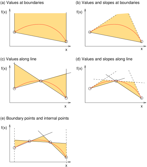
A.3 A sum rule for the enzymatic costs of combined flux profiles

The sum rules for enzymatic flux cost functions, Eqs (5) and (7), follow from Euler’s theorem on homogeneous functions.

Eq. (5) implies that the flux point cost $\frac{\partial a^{\rm enz}}{\partial v_{l}}v_{l}$ is equal to the enzyme point cost $\frac{\partial h}{\partial e_{l}}\,e_{l}$ (proof in SI section E.6). Thus, for any flux profile ${\bf v}$, the enzymatic flux cost is given by the sum of enzyme point costs of all reactions; if the enzyme cost $h({\bf e})$ is linear, this sum is also equal to the absolute enzyme cost $h$. At first glance, Eq. (5) seems to state something obvious: that the enzyme cost $a^{\rm enz}({\bf v})=\sum_{l}h(e_{l})$ of a flux profile is given by the sum of all enzyme costs. However, the sum rule is not so obvious: the derivatives $\frac{\partial a^{\rm enz}}{\partial v_{l}}$ in the sum rule are not derivatives $\partial g^{\rm enz}_{l}({\bf v},{\bf m})/\partial v_{l}$ at fixed metabolite concentrations, but refer to optimised metabolite concentrations: they imply an optimal metabolic adjustment whenever fluxes are changing. This is what distinguishes our enzymatic flux cost function from simple additive flux costs as assumed in FBA with molecular crowding. Implicitly, these older methods assume a proportionality between enzyme levels and stationary fluxes, as if metabolite concentrations were constant and unaffected by changing enzyme levels and fluxes. Instead, our sum rule rightly assumes that fluxes and enyzme levels are coupled through (variable) metabolite levels.

A similar sum rule holds for flux profiles that are represented by convex combinations ${\bf v}=\sum\sigma_{\alpha}\,{\bf v}^{(\alpha)}$ of prototype flows ${\bf v}^{(\alpha)}$: now the cost of ${\bf v}$ is homogenous (with degree 1) with respect to the coefficients $\sigma_{\alpha}$, where the basis may be complete or even overcomplete:

$$a^{\rm enz}=\sum_{\alpha}\frac{\partial a^{\rm enz}}{\partial\sigma_{\alpha}}\,\sigma_{\alpha}$$ (15)

for the coefficients $\sigma_{\alpha}$. The derivatives are given by $\frac{\partial a^{\rm enz}}{\partial\sigma_{\alpha}}=\sum_{l}\frac{\partial a^{\rm enz}}{\partial v_{l}}\frac{\partial v_{l}}{\partial\sigma_{\alpha}}=\frac{\partial a^{\rm enz}}{\partial{\bf v}}\cdot{\bf v}^{(\alpha)}$. Again, there is an analogous sum rule for scaled flux costs.

Similar sum rules hold for optimal metabolite or enzyme levels as functions on the flux polytope:

$$\sum_{l}\frac{\partial c_{i}^{\rm opt}}{\partial\ln v_{l}}=\sum_{l}\frac{\partial c_{i}^{\rm opt}}{\partial v_{l}}\,v_{l}=0.$$

$$\sum_{l}\frac{\partial e_{l}^{\rm opt}}{\partial\ln v_{l}}=\sum_{l}\frac{\partial e_{l}^{\rm opt}}{\partial v_{l}}\,v_{l}=e_{l}^{\rm opt}.$$ (16)

A.4 Linear and nonlinear approximations of enzymatic flux cost functions

To obtain realistic linear flux cost functions, we consider the enzymatic flux cost and linearise it around a prototype flux profile ${\bf v}^{\rm pt}$. This approximation works best near the prototype flux profile (or, more precisely, for flux profiles ${\bf v}$ that favour similar metabolite profiles as the prototype flux profile). Therefore, we should chose a prototype flux profile ${\bf v}^{\rm pt}$ that is “typical”, resembling the flows at which $a^{\rm enz}({\bf v})$ will be evaluated. To compute the linear cost weights, we start from the cost gradient in a point ${\bf v}$,

$$a^{\rm enz}_{v_{l}}=\frac{\partial a^{\rm enz}({\bf v})}{\partial v_{l}}=\frac{h_{e_{l}}\,e^{\rm opt}_{l}({\bf v})}{v_{l}}=\frac{h_{e_{l}}}{k^{\rm pt}_{l}},$$ (17)

where $e^{\rm opt}_{l}({\bf v})$ is the enzyme profile that is favoured by our flux profile ${\bf v}$ (see SI E.9 and E.6). Equation (17) holds also for kinetic flux cost functions (with a direct metabolite cost). By linearising the cost function around a prototype state ${\bf v}^{\rm ref}$, we obtain the linear approximation

$$a^{\rm enz}({\bf v})=\sum_{l}\frac{\partial a^{\rm enz}}{\partial v_{l}}\,\,v_{l}\approx\sum_{l}\left(\frac{\partial a^{\rm enz}}{\partial v_{l}}\right)_{{\bf v}^{\rm pt}}\,\,v_{l}=\sum_{l}a^{\rm enz}_{v_{l}}\,v_{l}$$ (18)

with the cost weights $a^{\rm enz}_{v_{l}}$. There is no offset term, and so our approximated cost function is again linearly scalable. The formula (18) holds only for non-negative fluxes. For other flux profiles, with negative fluxes, we may reorient the reactions and obtain the same formula, but with different prefactors (each obtained from a different prototype flux profile). The signs of these prefactors must match the flux signs. If we assume the same (absolute) prefactors for all F-cones, we obtain the formula $a^{\rm lin}({\bf v})=\sum_{l}a_{v_{l}}\,|v_{l}|$, the typical cost function in FBA with weighted flux minimisation.

Quadratic approximation of the enzymatic flux cost The linear approximation (18) can provide us with linear flux cost weights for linear FCM or FBA with molecular crowding. As expected, the linearised flux cost is exact for the prototype flux profile and scaled versions of it. For other flux profiles, there is an approximation error which depends on how much the catalytic rates ($v_{l}/e_{l}$, for optimised enzyme levels) differ between ${\bf v}$ and the prototype flux profile ${\bf v}^{\rm pt}$. For a more accurate, nonlinear approximation of the flux cost $a^{\rm enz}({\bf v})$, we use several prototype flux profiles ${\bf v}^{(\alpha)}$. We first approximate our flux profile ${\bf v}$ by a convex combination ${\bf v}\approx\sum_{\alpha}\sigma_{\alpha}\,{\bf v}^{(\alpha)}$ of the prototype flux profiles (with positive weights $\sigma_{\alpha}$ satisfying $\sum_{\alpha}\sigma_{\alpha}=1$). Using the same weights $\sigma_{\alpha}$, we define a weighted average of the inverse catalytic rates $1/r_{l}^{\prime}=\sum_{\alpha}\sigma_{\alpha}/r_{l}^{(\alpha)}$. This yields the approximated flux cost (proof in section E.10)

$$a^{\rm non}({\bf v})\approx\sum_{l}\frac{h_{e_{l}}}{r_{l}^{\prime}}\,v_{l}=\sum_{l\alpha}\frac{\sigma_{\alpha}}{r_{l}^{(\alpha)}}\,h_{e_{l}}\,v_{l}.$$ (19)

This cost function is nonlinear in ${\bf v}$ because the prefactors $1/r_{l}^{\prime}$ are weighted averages of the prototype flux profiles’ $1/r_{l}$, where the prefactors $\sigma_{\alpha}$ depend on ${\bf v}$. With a single prototype flux profile, the curvature vanishes and we reobtain the linear approximation. With more than one prototype flux profile, the cost function is quadratic (see section E.10). For a good approximation (19), it may be better to use fewer prototype flux profiles, but to choose prototype flux profiles that that favour similar metabolite profiles as the flux profiles at which the cost function will be evaluated.

Appendix B Mathematical properties of flux cost function

In this section, I study the conditions under which an enzymatic metabolite cost (or “briefly enzymatic M-cost”) functions have a unique optimum. Then, I show that enzymatic flux cost functions are concave on the F-cone and strictly concave on the interpolation line between kinetically distinct flux profiles.

B.1 Shape of the enzymatic metabolite cost function

Conditions for a strictly convex metabolite cost function An enzymatic M-cost function is called “regular” if it is strictly convex on the metabolite polytope. Generally, in a given point of the M-polytope, the enzymatic M-cost will be positively curved in some directions and constant in others. These “cost-neutral” directions depend on network structure and rate laws in the model. To study this further, we consider cost curvature matrix $\mathbf{H}$, the Hessian matrix of the enzymatic M-cost function. If $\mathbf{H}$ is positive definite (i.e. regular) in all points of the M-polytope, the enzymatic M-cost is strictly convex and the ECM problem has a unique solution. By contrast, if $\mathbf{H}$ has vanishing eigenvalues (i.e. it is singular), the enzyme cost is non-strictly convex and the ECM problem has a larger set of optimal solutions. To see whether $\mathbf{H}$ is regular, we need to determine the cost-neutral subspace of our model.

Shape of the enzymatic metabolite cost function Each feasible flux profile ${\bf v}$ defines a polytope of feasible metabolite profiles, and each metabolite profile ${\bf m}$ in this M-polytope defines an enzyme profile, and thus metabolic state. The enzymatic M-cost function on the M-polytope further defines which of these states are optimal. There are two cases: in the regular case, an M-cost function is strictly convex, with a regular cost curvature matrix on the entire M-polytope, leading to a single optimal metabolite profile. In the singular case, some directions in metabolite space are cost-neutral (i.e. the cost curvature matrix has a non-empty nullspace), leading to a continuous set, or subpace, of optimal metabolite profiles. What case we are in depends on network structure and rate laws considered. As a criterion, we search for “cost-neutral” metabolite variations $\delta{\bf m}$ that leave enzymatic M-cost unchanged.

Cost-neutal variations and the nullspace of the cost curvature matrix Let us have a closer look at the enzymatic M-cost $g^{\rm enz}({\bf m})$ and its curvature matrix $\mathbf{H}({\bf m})$. The nullspace of $\mathbf{H}$ is called $\mbox{Ker}(\mathbf{H})$. In models with factorised rate laws, $\mathbf{H}$ has the following properties:

1. $\mathbf{H}$ is positive semidefinite (proof in SI E.4).

2. Given a flux profile ${\bf v}$, the cost curvature matrix $\mathbf{H}$ in a point ${\bf m}$ is a sum of matrices for the individual reactions $\mathbf{H}({\bf m};{\bf v})=\sum_{l}\mathbf{H}^{(l)}({\bf m};{\bf v})$. Each of these matrices is positive semidefinite (because the enzymatic metabolite cost for each reaction is convex), and so the nullspace of $\mathbf{H}$ is the intersection of these nullspaces of the matrices $\mathbf{H}^{(l)}$. If this intersection is empty, $\mathbf{H}$ will be regular. This is the case in all models with CM rate laws (proof in section E.5).

3. The nullspace of $\mathbf{H}$ is structurally determined, i.e. determined by rate laws, network structure, and the flux pattern of ${\bf v}$ (with strictly defined zero values). It is independent of the specific choices of ${\bf m}$ and ${\bf v}$.

4. Let ${\bf v}_{\rm A}$ and ${\bf v}_{\rm B}$ be flux modes with identical flux profile patterns, and ${\bf m}_{\rm A}$ and ${\bf m}_{\rm B}$ be the favoured metabolite profiles of ${\bf v}_{\rm A}$ and ${\bf v}_{\rm B}$. Then the cost curvature matrices in the points $({\bf v}_{\rm A},{\bf m}_{\rm A})$ and $({\bf v}_{\rm B},{\bf m}_{\rm B})$ have identical nullspaces.

5. In models with reversibility-based rate laws [10], $\mbox{Ker}(\mathbf{H})$ is the nullspace of the transposed stoichiometric matrix ${\bf N}^{\top}$; in models with saturation-based rate laws, $\mbox{Ker}(\mathbf{H})$ is the nullspace of the molecularity matrix ${\mathbf{M}^{\rm S}\choose\mathbf{M}^{\rm P}}$; in models with CM rate laws, $\mbox{Ker}(\mathbf{H})$ is empty, i.e., $\mathbf{H}$ is regular (proof in section E.5).

Conditions for singular enzymatic M-cost functions Under what conditions is the optimal metabolite profiles non-unique? Two metabolite profiles ${\bf m}_{\rm A}$ and ${\bf m}_{\rm B}$ are called cost-equal if their difference vector ${\bf m}_{\rm A}-{\bf m}_{\rm B}$ is cost-neutral, i.e. located in the cost-neutral subspace (i.e. the nullspace of $\mathbf{H}$). As a criterion for metabolite profiles being cost-equal, we introduce another helpful concept, the notion of be rate-equal,

Given the enzyme concentrations $e_{l}=1$, a metabolite profile ${\bf m}_{\rm A}$ yields the flux distribution ${\boldsymbol{\nu}}({\bf m},\mathbf{1})$ (which may be non-stationary). We now ask whether moving from ${\bf m}_{\rm A}$ to ${\bf m}_{\rm B}$, at fixed enzyme levels, changes this flux distribution or not. If there is no change, ${\bf m}_{\rm A}$ and ${\bf m}_{\rm B}$ are called rate-equal, otherwise they are called rate-distinct. Rate-equal metabolite profiles are cost-equal.

Using this notion, we obtain the following results:

1. If a metabolite (with index $i$) has no influence on any of the reaction rates. In this case, any variation vector of the form $\delta{\bf m}=(0,0,..,\delta m_{i},0,0)^{\top}$ is a nullvector of $\mathbf{H}$.

2. If the rate laws do not directly depend on metabolite concentrations, but on the thermodynamic forces, which are given by $\theta_{l}=\ln k^{\rm eq}_{l}-\sum n_{il}\,\ln c_{i}$. If the rate laws depend on these forces only (which holds, e.g. for the “reversibility-based” rate laws in [10]), then any variation $\delta{\bf m}$ that leaves the driving forces unchanged is a nullvector of $\mathbf{H}$. Such vectors $\delta{\bf m}$ are given by the nullvectors of ${{\bf N}^{\rm tot}}^{\top}$ (i.e. conserved moiety vectors).

3. If the rate laws do not directly depend on metabolite concentrations, but only on mass-action products. The mass-action products are given by $\prod_{i}\,c_{i}^{m^{S}_{li}}$ (for reaction substrates) or $\prod_{i}\,c_{i}^{m^{P}_{li}}$ (for reaction products), with molecularities in the matrices $\mathbf{M}^{S}$ and $\mathbf{M}^{P}$ (e.g. the saturation-based rate laws in [10]). Variations $\delta{\bf m}$ that do not affect the mass-action products are nullvectors of $\mathbf{H}$. Such vectors $\delta{\bf m}$ are given by the nullvectors of ${\mathbf{M}^{S}\choose\mathbf{M}^{P}}$.

4. If there exist variation vectors $\delta{\bf m}$ that do not affect any reaction rates, the enzyme cost function of a reaction $l$ defines, in each point of the M-polytope, a cost curvature matrix $\mathbf{H}^{(l)}$ with a nullspace $\mbox{Ker}(\mathbf{H}^{(l)})$. The nullspace of $\mathbf{H}$ (for the sum of all enzyme costs) is the intersection of all these nullspaces. A metabolite variation that is cost-neutral for all reactions is therefore a nullvector of $\mathbf{H}$. In contrast, if any possible variation $\delta{\bf m}$ affects at least one reaction, then $\mathbf{H}$ is regular.

To summarise, nullvectors of the cost curvature matrix can arise structurally and depedn only on rate laws and network structure. For models with factorised rate laws (and with non-constant thermodynamic and kinetic efficiency factors), the entire nullspace of the cost curvature matrix is determined in this way. This is stated by the following lemma (proof in SI section E.1).

Lemma 1

The nullspace of the enzymatic metabolite cost curvature matrix is given by the cost-neutral subspace In models with factorised rate laws and non-constant thermodynamic and kinetic efficiency factors, all neutral metabolite variations $\delta{\bf m}$ are nullvectors of the cost curvature matrix $\mathbf{H}$. Conversely, all nullvectors of $\mathbf{H}$ are neutral metabolite variations. This holds in any point ${\bf m}$ of the M-polytope. A nullvector of $\mathbf{H}$ in a point ${\bf m}$ is also a nullvector of $\mathbf{H}$ in any other point.

According to this lemma, the nullspace of the cost curvature matrix for a given kinetic model (i.e. network structure, rate laws, and model parameters) and a predefined flux pattern is structurally determined: it is independent of the metabolite profile ${\bf m}$ and the flux profile ${\bf v}$. If the cost-neutral subspace is empty, then according to Lemma 1 the enzymatic M-cost is regular (i.e. strictly convex on the M-polytope) and the ECM problem has a unique solution. This holds for all models with common modular rate laws because their cost-neutral subspace is empty in fact (proof in section E.5).

B.2 Enzymatic flux cost functions are concave on the F-cone

Lemma 2

Concave flux cost functions (proof in section E.2). We consider a cost function $f({\bf m};{\bf v})$ scoring a metabolite profile ${\bf m}$ (in the M-polytope)and a flux profile ${\bf v}$ (in the F-cone). Let the cost function be linear in the fluxes, $f({\bf m};\alpha\,{\bf v}_{\rm A}+\beta\,{\bf v}_{\rm B})=\alpha\,f({\bf m};{\bf v}_{\rm A})+\beta\,f({\bf m};{\bf v}_{\rm B})$, and bounded from below (e.g. it is positive). Let $g({\bf m})$ be a cost function on the M-polytope that is bounded from below. Under these conditions, the flux cost function $a({\bf v})=\min_{{\bf m}\in{\mathcal{P}}_{\rm F}}f({\bf m};{\bf v})+g({\bf m})$ is concave on the F-cone ${\mathcal{P}}_{\rm F}$. This lemma also holds if $f$ (for each given ${\bf m}$) is not linear, but concave in the fluxes.

From Lemma 2, we obtain

Proposition 2

(Enzymatic and kinetic flux cost functions are concave) Let $h({\bf e})$ be a linear enzyme cost function, and let $g({\bf m})$ be a metabolite cost function, both bounded from below. We defined the enzymatic M-cost $g^{\rm enz}({\bf m};{\bf v})=h({\bf e}({\bf m};{\bf v}))$. Then the enzymatic flux cost $a^{\rm enz}({\bf v})=\min_{\bf m}g^{\rm enz}({\bf m};{\bf v})$ and the kinetic flux cost $a^{\rm kin}({\bf v})=\min_{\bf m}g^{\rm enz}({\bf m};{\bf v})+g({\bf m})$ are concave functions on the F-cone.

Remarks

1. “Bounded from below” means that costs cannot got to $-\infty$. This holds for all positive cost functions (assuming that fitness terms are represented on absolute, not on logarithmic scale).

2. Linear enzyme cost function Lemma 2 holds also for to the enzymatic M-cost $g^{\rm enz}({\bf m};{\bf v})$, because it is linear in the fluxes (since the enzyme level appears linearly in the rate laws) and because the enzyme cost function $h({\bf e})$ is assumed to linear. In contrast, if $h({\bf e})$ were nonlinear and convex, the resulting flux cost function might not be concave. In case $h({\bf e})$ is nonlinear and concave, Lemma 2 and proposition 2 will still hold, but the M-cost may no further be convex.

3. Non-stationary fluxes Proposition 2 holds for any flux distributions, stationary or non-stationary ones. However, the flux distributions ${\bf v}_{\rm A}$ and ${\bf v}_{\rm B}$ and all their interpolations must be thermo-physiologically feasible (i.e. thermodynamically feasible given the metabolite concentration ranges and predefined concentrations assumed in our model). A thermo-physiologically feasible flux pattern defines an orthant in flux space. If non-stationary flux distributions are allowed, then any flux distribution in this orthant can be a solution. Since the flux cost is concave on this orthant, it is also concave on all B-polytopes within the orthant.

B.3 The enzymatic flux cost function is strictly concave between kinetically distinct flux profiles

Depending on the model, the enzymatic flux cost may not only be concave, but even be strictly concave on the B-polytope: that is, adding two flux profiles yields an additional positive compromise cost. For a cost function to be strictly concave, all flux profiles on the B-polytope must be kinetically distinct.

Definition B.1

Kinetically distinct metabolic flux profiles Consider two flux profiles ${\bf v}_{\rm A}$ and ${\bf v}_{\rm B}$ with the same flux pattern (i.e. with the same active reactions and flux directions). The flux profiles are called kinetically distinct (for the kinetic model in question) if ${\bf v}_{\rm A}$ and ${\bf v}_{\rm B}$ have no optimal metabolite profile in common.

Remark If the enzymatic M-cost function is regular (i.e. if each flux profile favours only a single metabolite profile), then flux profiles with different optimal profiles are kinetically distinct. If the enzymatic M-cost function is singular (i.e. if flux profiles favour several metabolite profiles), no metabolite profile may be favoured by both of the flux profiles.

Lemma 3

We consider a kinetic model with a given flux pattern defining an M-polytope and a benefit function defining a B-polytope. If the enzymatic M-cost function is strictly convex on the interior of the M-polytope, all flux profiles in the B-polytope are kinetically distinct.

Next, we can state that an enzymatic flux cost function is strictly concave on the B-polytope if (and only if) all flows in the B-polytope are kinetically distinct.

Lemma 4

(Conditions for strictly concave flux cost functions) Let $a^{\rm enz}({\bf v})$ be an enzymatic F-cost function on an F-cone. If two flux profiles ${\bf v}_{\rm A}$ and ${\bf v}_{\rm B}$ in the interior of this polytope are kinetically distinct, then $a^{\rm enz}({\bf v})$ is strictly concave on the line between ${\bf v}_{\rm A}$ and ${\bf v}_{\rm B}$ (proof in section E.4).

To prove this statement, we analyse the ECM problem in a metabolic model with given rate laws and flux directions. We assume that external metabolite concentrations are fixed and that the internal metabolite concentrations need to be optimised.

Lemma 5

If all flux profiles in the interior of a B-polytope are kinetically distinct, the enzymatic F-cost $a^{\rm enz}({\bf v})$ is strictly concave on the interior of this B-polytope.

Remarks

1. The proposition also holds for combinations of several flux profiles, ${\bf v}_{\rm A},{\bf v}_{\rm B},{\bf v}_{\rm C}$ … In this case, instead of a line we consider their convex hull, i.e. the simplex spanned by the flux profiles.

2. Kinetic flux cost functions (i.e. which contain enzymatic and direct metabolite costs) are strictly concave under the following conditions: the kinetic metabolite cost $g({\bf m})$ (i.e. enzymatic plus direct metabolite cost) must be convex, and its cost curvature matrix must have the same nullspace everywhere in the M-polytope. In this case, adding the direct metabolite cost to the enzymatic M-cost may change the cost curvature matrices, but these matrices, in the entire M-polytope, will still have the same nullspaces. Therefore the concavity proof in SI E.4 still applies.

By combining Lemma 3 and Lemma 5, we obtain the following proposition.

Proposition 3

We consider a kinetic model with a predefined flux pattern and a benefit function defining an M-polytope and a B-polytope. If the enzymatic M-cost is strictly convex on the interior of the M-polytope, the enzymatic F-cost $a^{\rm enz}({\bf v})$ is strictly concave on the interior of the B-polytope.

In a typical model, different flux profiles are kinetically distinct, i.e. they favour different metabolite profiles. If they are not kinetically distinct, the flux cost function varies linearly on the line between them.

1. Flux profiles that differ only by scaling The enzymatic flux cost scales linearly with the flux profile. If two flux profiles ${\bf v}_{\rm A}$ and ${\bf v}_{\rm B}$ differ only scaling, the flux cost is linear, and therefore not strictly concave on the interpolation line between them. However, such pairs of differently scaled flux profiles cannot occur in the same B-polytope

2. Flux profiles that differ only in the usage of isoenzymes Let us consider all enzyme molecules that catalyse a reaction R and split them arbitrarily into two pools (E1, “blue” enzyme molecules) and (E2, “red” enzyme molecules), thus representing our original reaction by two separate “isoreactions” with identical sum formulae and kinetics: R1 (catalysed by blue enzyme) and R2 (catalysed by red enzyme). Since this splitting is arbitrary, it can neither change the system dynamics nor the resulting flux cost. This means that the flux cost remains additive between the isoreactions R1 and R2, and is therefore not strictly concave.

In these two examples, the flux profiles ${\bf v}_{A}$ and ${\bf v}_{\rm B}$ favour the same metabolite profile: therefore, the interpolated flux profiles can be optimally realised by linearly interpolating the enzyme levels. With a linear cost function $h({\bf e})$, this implies an additive cost between ${\bf v}_{\rm A}$ and ${\bf v}_{\rm B}$. But what if the optimal metabolite profile of a flux profile is not unique, and therefore two flux profiles may be (but do not have to be) realised by the same profiles – will strict concavity still hold?

1. Flux profiles that favour kinetically equal metabolite profiles. In some models, there exist different metabolite profiles ${\bf m}_{\rm A}$ and ${\bf m}_{\rm B}$ that yield exactly the same reaction rates (with enzyme levels kept constant), and this may even hold for any metabolite profiles on the line between ${\bf m}_{\rm A}$ and ${\bf m}_{\rm B}$. In this case, the solution of the ECM problem will be non-unique. Here is an example: consider a chain of reactions A $\Leftrightarrow$ B + C $\Leftrightarrow$ D with reversible mass-action kinetics. If [B] is scaled by a factor 10 and [C] is scaled by 0.1, the reaction rates remain constant. And due to the logarithmic scale in the metabolite polytope, any convex conbination of the two metabolite profiles yield the same rates (and in ECM the same enzymatic M-cost). In fact, the enzymatic M-cost cost is constant on an entire subspace in log-metabolite space, as indicated by a nullvector of the cost curvature matrix of $g^{\rm enz}({\bf m};{\bf v})$.

2. Metabolites that do not affect the reaction rates As an approximation, we may consider models in which some reaction rates do not depend on any metabolite concentrations. This holds, for example, if enzymes are assumed to be substrate-saturated and completely forward-driven, an approximation made by the capacity-based rate laws [10]. If such rate laws are used, even small enzyme perturbations can completely impair a steady state. In such models, it is also likely that some metabolites have no impact on any reaction rate. A similar case occurs when metabolites formally belong to a model, but do not participate in any reactions.

In these two examples, two flux profiles can favour the same metabolite profiles, but also other metabolite profiles because the optimal metabolite profiles are not unique. In this case, when interpolating between two flux profiles, one could obtain different metabolite profiles and still realise the flux changes by linear changes in enzyme levels (i.e. at varying metabolite levels, but constant catalytic rates!). Therefore, whenever two flux profiles can favour the same metabolite profiles, we define them as not kinetically distinct.

B.4 The optimum points of concave flux cost functions are polytope vertices

Figure 7: Elementary and non-elementary B-polytope vertices. (a) Simple branch point model (top) with four elementary flux modes (EFMs; bottom); in the model all fluxes are constrained to be positive. (b) Metabolic flux profiles as points in flux space (three of the four dimensions are shown, referring to reactions 1, 2, and 3). The cone of feasible flux profiles is spanned by the four EFMs. A predefined benefit value (in the example, $v_{2}+v_{3}=\mbox{\rm const.}$) defines a plane that intersects the cone and yields the B-polytope (blue rectangle) or feasible flux profiles. The vertices of this B-polytope correspond to EFMs. (c) If we add an upper bound on $v_{2}$, some of the flux profiles are discarded; a part of the B-polytope (red rectangle) is cut off and two non-elementary vertices emerge (blue circles).

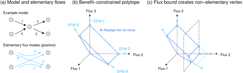
If all flux profiles in a B-polytope are kinetically distinct, the optimal (i.e. enzyme-cost-minimising) flux profile must be a polytope vertex if this optimum unique. Otherwise, at least one of them must be a polytope vertex (and they all lie on a line, plane, or hyperplane). For the proof, we regard the F-cone as a closed set and continue the flux cost function – which is continuous inside the F-cone – to flux cone boundaries, including all vertices. After a proof for this function, we will handle the remaining cases in which the flux cost function is discontinuous between an F-cone and one of its boundaries.

A concave flux cost function has an optimum point in a polytope vertex The enzymatic flux cost function on a B-polytope has a global minimum in one of the polytope vertices. The same minimal value can occur in non-vertex points. We can see this as follows. Any polytope point ${\bf v}$ can be written as a convex combination $\sum_{\alpha}\sigma_{\alpha}{\bf v}_{(\alpha)}$ of the vertices. If the flux cost function is concave on the B-polytope, the cost $a({\bf v})$ in a point ${\bf v}$ must be at least as high as the combined cost $\sum_{\alpha}\sigma_{\alpha}a({\bf v}_{(\alpha)})$ of the vertex points, and this combined cost must be at least as high as the lowest cost $\mbox{min}_{\alpha}a({\bf v}_{(\alpha)})$ among the vertices. Thus, if an inner point ${\bf v}$ achieves the minimum cost, there must also be a vertex point with the same minimum cost.

Strictly concave flux cost functions have minimum points only on polytope vertices If the enzymatic flux cost function is strictly concave on the B-polytope, all its minimum points must be polytope vertices.

A complication: discontinuity at polytope boundaries Above, we assumed that the enzymatic flux cost is continuous on the entire (closed) F-cone, including boundary points such as vertices. However, for proving that flux cost functions must be concave, we consider flux profiles with identical flux patterns (including zero values). Geometrically, these proofs apply only to the interior of an F-cone, which is an open set, and may not hold for points on the polytope boundary. In fact, we saw that flux cost functions show jumps at the polytope boundaries, i.e. if two neighbouring polytopes share a vertex point, then for one of them the cost function will not be continuous in this point. That is, we may have to compare a flux profile from the interior of an F-cone to a flux profile on the polytope boundary, which already shows a jump. Unfortunately, the conclusion about minimum points of a flux cost function concerns polytope vertices, which are boundary points! Thus, to claim that vertex points are optimal, we need to reformulate the problem: we consider the flux cost function on the interior of the F-cone and define the continuous continuation of this function, which includes all points on the polytope boundary. According to our previous argument, this continued function will have its minima in polytope vertices! Now it is true that the actual cost function value in a vertex point may differ from the value of the “continued” function. But for optimality reasons, the actual cost function cannot be higher than the continued function, so the vertex point will achieve an even lower minimum value. Therefore, our conclusions about vertex points being optimal still hold.

B.5 Condition for locally optimal flux profiles

Definition B.2

Locally optimal flux profile. A flux profile is locally optimal if it has a lower (or equal) flux cost than any other flux profile in a small region around ${\bf v}$ within the B-polytope.

Proposition 4

(“Manu’a criterion”) A B-polytope vertex ${\bf v}$ is locally optimal if it has a unique favoured metabolite profile ${\bf m}$ and if it is the only favoured flux profile of this profile ${\bf m}$ (proof in section E.7).

Remark Proposition 4 suggests a construction algorithm for locally optimal states (“Manu’a algorithm”): (i) Start from some initial flux profile (e.g. obtained by linear FCM). (ii) Use ECM to compute the favoured metabolite profile. (iii) Compute the catalytic rates, use them to define a linear FCM problem, and solve it for the optimal flux profile. (iv) Iterate steps number (ii) and (iii), until convergence. In the end, check the resulting favoured metabolite profiles and flux profiles for uniqueness. The flows computed by linear FCM are likely to be sparse (in models without flux constraints, they will be EFMs); therefore, some metabolite concentrations (e.g. within inactive pathways) may be undetermined. This non-uniqueness can be resolved by regularisation during the ECM steps.

(a) Schematic explanation                  (b) Simulation results for branch point model

Figure 8: For a flux to change its direction, metabolite and enzyme levels must change abruptly. (a) Schematic explanation. Curves show an enzymatic M-cost function (y-axis) for one of the metabolites (log-concentration on x-axis) ). The dark blue curve shows the enzymatic cost of the reaction that changes its flux direction. The light blue curve shows the sum of all enzymatic costs in other reactions. Their sum (red curve) determines the optimal metabolite concentration (dot, x-coordinate) and the optimal enzyme cost (dot, y-coordinate). If the flux is positive (top diagram), low metabolite concentrations are thermodynamically impossible (shaded region). In the plots below, the flux decreases and changes to negative values. The cost of this reaction changes accordingly, while the other costs remain almost constant (a realistic assumption, if we consider flux profiles close to a flux reversal). Exactly at the flux reversal, our reaction has a zero flux and no cost, and the optimal metabolite concentration is determined by the other reactions. In the following state, with an (infinitesimally small) negative flux, the metabolite concentration must be below the threshold value. This requires a jump in the metabolite concentration, and therefore in enzyme levels and enzyme cost. (b) Simulation results from the branch point model (see Figure 4), showing the same effect.

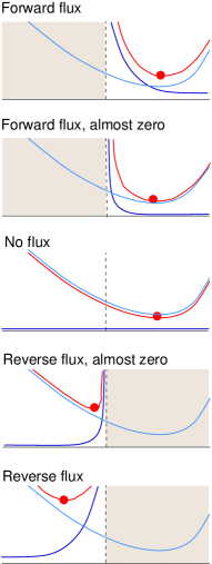
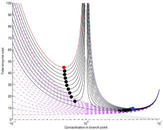
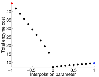
B.6 Flux cost close to a flux reversal

We saw that the enzymatic flux cost function is concave on each F-cone, i.e. for a given flux pattern. What shape will the cost function have on the entire flux space? If any feasible flux patterns are allowed, we merge all feasible F-cones and obtain a non-convex polytope and an F-cost on this set. What happens at the boundaries, where F-cones touch, and where fluxes change their directions? Will the cost function remain concave, smooth, or at least continuous?

For each flux mode, the enzymatic flux cost increases proportionally with the flux profile, so in the point ${\bf v}=0$ the flux cost increases in all directions with non-zero slopes. If we approach this point from different directions, we obtain different gradients, so the flux cost is not differentiable in this point. Moreover, the kinetic flux cost function (which contains direct metabolite costs) is not even continuous in this point; it converges to different values when approaching ${\bf v}=0$ from different directions. This shows that that quadratic flux cost functions such as $\sum_{l}v_{l}^{2}$, are not very realistic, and that piecewise linear cost functions, i.e. linear flux cost functions on each F-cone, are a better choice.

For a reaction flux to change its direction, the mass-balance ratio of substrates and products must change. This can be achieved by a change in external metabolite concentrations (i.e. model parameters) or by changes in internal metabolite concentrations (which follow from enzyme adaptations to other parameter changes). To study the shape of the flux cost function at the polytope boundaries, we consider again our branch point model from Figure 4. If all three reactions are active, there are $2^{3}=8$ possible flux profile patterns, corresponding to the eight orthants in flux space. The plane of stationary fluxes intersects six of these orthants. The other two orthants can be discarded, because the flux patterns in these orthants would lead to accumulation or depletion of the branch point metabolite. The flux directions are directly determined by chemical potential differences: e.g. a positive flux $v_{1}$ in Figure 4 requires that $\mu_{X}>\mu_{c}$. For simplicity, let us assume that $\mu_{x}>\mu_{y}>\mu_{z}$ (this only depends on the external metabolite concentrations). Two possible choices of $\mu_{c}$ lead to stationary flux profiles: if $\mu_{c}$ is lower than $\mu_{x}$ and higher than $\mu_{y}$, all fluxes run in forward direction; and if it is lower than $\mu_{x}$ and higher than $\mu_{y}$, the flux $v_{2}$ is reversed. Thus only two of the orthants remain feasible (blue or red), and the choice between them depends on the chemical potential $\mu_{c}$. The flux cost is a function on one of the two coloured triangles. With a predefined objective (e.g. flux $v_{3}$), we obtain the two B-polytopes (thick black line in Figure 8). Within each part of the line (blue or red), the cost function is concave. Between the two polytopes, the flux cost function shows a jump (see Figures 8 and 9). Between two F-cones, the enzymatic flux cost function is not continuous, except for some unlikely cases (requiring fine-tuned model parameters). Also the metabolite concentrations, enzyme levels, and enyme cost show jumps in their values. The jumps in the optimal metabolite and enzyme levels, as we move smoothly between the polytopes, indicate a zeroth-order phase transition.

Generally, a flux reversal requires a change of the thermodynamic driving force (and, thus, of metabolite concentrations). At the point of reversal, the metabolic flux profile crosses the boundary between two F-cones and moves to another segment of flux space. At the same time, in metabolite space the feasible metabolite polytope flips along the boundary associated with the reversed reaction (see Figure 9) and the metabolite profile jumps to a new polytope.

Figure 9: Metabolite profiles during flux reversal. The drawings show enzymatic cost functions on the metabolite polytope (schematic examples). Physiological and thermodynamic constraints are shown by dashed lines, enzymatic M-cost by colours from bright (low) to dark (high). Compare Figure 8 for a one-dimensional example. (a) A flux change without flux reversal leaves the metabolite polytope unchanged. The shape of the cost function changes, and the optimum point moves. (b) In a flux reversal, a flux changes from forward direction to a zero value and further to backward direction, each time defining a different M-polytope. At the point of flux reversal (centre), the cost barrier disappears, but the optimum point remains in the lower sub-polytope. After the reversal, at a slightly negative flux, this optimum becomes inaccessible and another point, near the boundary of the new M-polytope, becomes optimal. At larger negative fluxes, the optimum moves further away from the boundary (not shown).

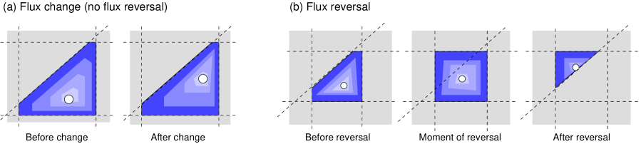B.7 The trajectory of optimal metabolite profiles for a sweep between two metabolic flux profiles

Figure 10: Trajectory of the optimal metabolite profiles as we interpolate between flux profiles Trajectory of optimal metabolite profile during a flux sweep. In each point of the trajectory the gradients of the two original cost functions point in opposite directions. Given the two cost functions (blue and red contours), this condition defines the trajectory shape. The trajectory remains inside the grey region, defined by the contour line of function A passing through the point ${\bf m}_{{\rm B}}$ and by the contour line of function B passing through the point ${\bf m}_{{\rm A}}$.

If we interpolate between flux profile ${\bf v}_{\rm A}$ and flux profile ${\bf v}_{\rm B}$ in flux space, how will the optimal metabolite profile move in metabolite space? We assume that the two flux profiles are in the same B-polytope (i.e. no reaction flux changes its sign) and that the ECM problem is regular, i.e. with a unique solution for each of the flux profiles. In this case, the metabolite profile will move along a continuous trajectory between the two optimal points ${\bf m}_{\rm A}={\bf m}^{\rm opt}({\bf v}_{\rm A})$ and ${\bf m}_{\rm B}={\bf m}^{\rm opt}({\bf v}_{\rm B})$. Each trajectory point is the optimum point for some interpolated flux profile $\sigma\,{\bf v}_{\rm A}+(1-\sigma)\,{\bf v}_{\rm B}$: the optimality condition $\nabla_{{\bf m}}\sigma\,g^{\rm enz,{\bf v}_{\rm A}}+(1-\sigma)\,g^{\rm enz,{\bf v}_{\rm B}}=0$ implies that in each trajectory point the gradients of the original cost functions $g^{\rm enz,{\bf v}_{\rm A}}$ and $g^{\rm enz,{\bf v}_{\rm B}}$ must be exactly in opposite directions.

We can compute the direction of the trajectory in its end points (e.g. in the optimum point for $g^{\rm enz,{\bf v}_{\rm A}}$.), for example, in the point ${\bf m}_{\rm A}$: with an infinitesimal interpolation parameter ${\rm d}\lambda$, we obtain a displacement ${\rm d}{\bf m}$ of the optimal profile. In the new point, the optimality condition reads, to second order

$$(1-{\rm d}\lambda)(\underbrace{\nabla q_{\rm A}}_{0}+\mathbf{H}_{\rm A}\,{\rm d}{\bf m})+{\rm d}\lambda(\nabla q_{\rm B}+\mathbf{H}_{\rm B}\,{\rm d}{\bf m})=0$$

$$\Rightarrow\mathbf{H}_{\rm A}\,{\rm d}{\bf m}+{\rm d}\lambda\,\nabla q_{\rm B}=0$$

$$\Rightarrow{\rm d}{\bf m}/{\rm d}\lambda=-\mathbf{H}_{\rm A}^{-1}\,\nabla q_{\rm B}.$$ (20)

Higher-order terms have been omitted, and the gradients $\nabla q_{\rm A}$ and $\nabla q_{\rm B}$ and the curvature matrices $\mathbf{H}_{\rm A}$ and $\mathbf{H}_{\rm B}$ are evaluated in the point ${\bf m}_{\rm A}$. The same argument can be applied to any point on the curve.

Appendix C Metabolic optimality problems

C.1 Flux benefit maximisation

In flux benefit maximisation (Figure 11) we maximise a linear flux benefit $b({\bf v})$ under the constraint ${\bf N}^{\rm int}\,{\bf v}=0$ and under one or several protein constraints $\forall r:a_{r}({\bf v})\leq a_{r}^{\rm max}$ (where $r$ denotes, e.g. density constraints for different cell compartments). Without loss of generality, we can assume that fluxes are non-negative, ${\bf v}\geq 0$. In practice, to solve this problem we consider scaled flux profiles $\hat{\bf v}$ with a nominal benefit $b=1$. This assumption, together with stationarity and flux sign constraints, restricts our flux profiles to a B-polytope defined by $b(\hat{\bf v})=1$. For each scaled flux profile $\hat{\bf v}$, we then compute the maximal scaling factor $\sigma$ at which $\forall r:a_{r}(\sigma\,\hat{\bf v})\leq a_{r}^{\rm max}$ is still satisfied. This maximal factor is exactly the maximal achievable benefit. We can further simplify this problem: since the enzymatic flux cost $a^{\rm enz}_{r}$ scales linearly with $\hat{\bf v}$, we need to maximize $\sigma$ such that $\forall r:\sigma\,a^{\rm enz}_{r}(\hat{\bf v})\leq a_{r}^{\rm max}$. The solution is $\sigma^{\rm opt}(\hat{\bf v})=\min_{r}\frac{a_{r}^{\rm max}}{a^{\rm enz}_{r}(\hat{\bf v})}$. If we perform the same optimisation on another B-polytope, with nominal benefit $b$, we obtain the same formula

$$b^{\rm opt}=\frac{1}{b}\,\sigma^{\rm opt}=\frac{1}{b}\min_{r}\frac{b\,a_{r}^{\rm max}}{a^{\rm enz}_{r}({\bf v})}=\min_{r}\frac{a_{r}^{\rm max}}{a^{\rm enz}_{r}({\bf v})}.$$ (21)

This means: the maximal achievable benefit, as a function on a B-polytope, is obtained by taking the minimum of all the functions $\frac{a_{r}^{\rm max}}{a^{\rm enz}_{r}({\bf v})}$. To find the optimum point, it is convenient to minimise the reciprocal benefit

$$1/b^{\rm opt}=\max_{r}\frac{a^{\rm enz}_{r}({\bf v})}{a_{r}^{\rm max}}$$ (22)

on the flux polytope. With a single protein constraint, this leads to exactly the same condition as our usual FCM problem (minimising a single enzyme cost function on the flux polytope). With several protein constraints, the problem become more involved. First, the protein functions cannot be determined by separate ECM problems. Instead, they must be be determined as solutions of an ECM problem that directly minimises $\max_{r}\frac{q_{r}({\bf m};{\bf v})}{a_{r}^{\rm max}}$. Since the maximum of two or more convex functions is convex, this is a convex (typically non-smooth) problem, but the cost functions $a^{\rm enz}_{r}({\bf v})$ on the flux polytope may have complicated shapes. Second, even if they were concave functions, the right-hand side of (22) (to be minimised) need not be concave, possibly giving rise to optimal flux profiles inside the flux polytope. Thus, we need to employ approximations. Approximating the cost functions $a^{\rm enz}_{r}({\bf v})$ by linear functions $a^{\rm enz}_{r}({\bf v})\approx{\bf a}^{(r)}_{{\bf v}}\cdot{\bf v}$, we obtain a linear optimality problem

$$\mbox{Minimise}_{z,{\bf v}}\quad z\quad\mbox{subject to} z\,{\bf a}_{r}^{\rm max}\geq\mathbf{A}_{{\bf v}}\cdot{\bf v},\quad{\bf N}^{\rm int}\,{\bf v}=0,\quad{\bf v}\geq 0.$$ (23)

This approximation can be used within an iterative optimisation method: we start from some initial flux state, linarise the protein demand functions around this state, solve the linear problem (23), and iterate these steps until convergence. The result is a local optimum. To find a global optimum, multiple runs with different starting points should be performed.

Figure 11: Flux benefit maximisation. (a) Protein constraints and benefit optimisation in flux space (schematic drawing). Two protein constraints (blue and red line) define a feasible region (shaded). Possible flux modes are defined by points on the B-polytope (diagonal lines) with a unit flux benefit (black line). For each of these points, the maximal flux benefit is given by the scaling factor that would move this point to the boundary defined by protein constraints. To compute this scaling factor, we need to solve a convex optimality problem in metabolite space. (b) Achievable benefit (i.e., scaling factor from (a)) as a function in flux space. The x-axis corresponds to the flux polytope (diagonal line in (a)). Top: red and blue lines show the possible scaling factor under one of the constraints. The scaling factor is defined by the minimum of the two functions (black line). The inverse achievable benefit is given by the maximum (black) of two concave functions (in fact, enzymatic cost functions), which itself is not concave.

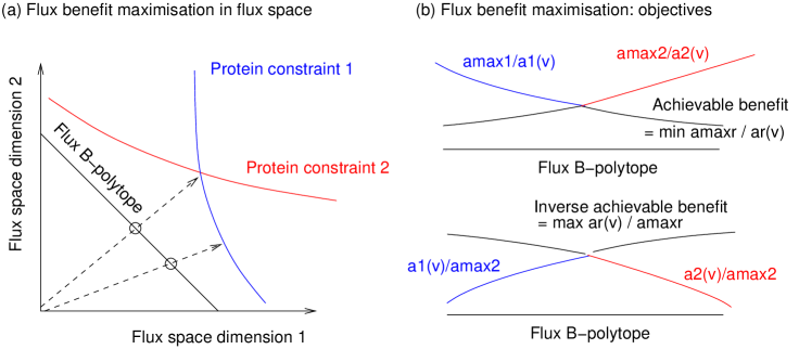
C.2 Optimisation of enzyme activity at given protein levels

When predicting optimal flux profiles, we usually assume that cells can choose, for each flux profile, the best possible enzyme profile. However, a cell may not be able to adjust its enzyme levels, at least not very quickly. To be prepared for fast, unpredictable changes, cells may employ express proteins preemptively: they produce enzyme for various possible situations and inhibit them posttranslationally. In [10], we showed that this problem – finding an enzyme profile that can realise a given number of flux distributions, and optimising this profile for minimal cost – can be formulated as a convex optimality problem. Here we consider a different scenario: we assume that the enzyme profile is given and that the cell needs to find a flux mode, realisable with these enzymes, that maximises the flux benefit (e.g. biomass production or substance conversion), where enzymes may be inhibited. What is the maximal possible flux benefit, the optimal metabolite profile, and what are the resulting enzyme activities in this case?

To answer this question, we replace the rate law

$$v_{l}=e_{l}\,k_{l}$$ (24)

by an inequality $v_{l}\leq e_{l}\,k_{l}$ (assuming that the actual reaction rates can be lower than what a non-inhibited enzyme could achieve). In our optimality problem, the enzyme profile ${\bf e}$ is given and we search for a flux profile ${\bf v}$ (and its log-metabolite profile ${\bf m}$) that maximise the benefit q ${\bf b}_{\rm v}\cdot{\bf v}$. To do so, we employ a trick: we only consider flux profiles ${\bf v}$ with a fixed nominal benefit $b={\bf b}_{\rm v}\cdot{\bf v}$ (which brings us back to an optimality problem on the B-polytope). We assume for each flux profile that the benefit can be scaled by a factor $\sigma$ and determine the maximal value $\sigma^{\rm opt}({\bf v})$ at which the enzyme constraint Eq. (24) can still be satisfied. A higher value of $\sigma^{\rm opt}$ means that the nominal benefit $b$ can be achieved at lower enzyme levels, or that a benefit time-integral $b\,\Delta t$ can be reached in a shorter period of time. To find the maximal scaling factor $\sigma^{\rm opt}$ for a flux profile ${\bf v}$, we

$$\mbox{Maximise}~{}\sigma\quad\mbox{s.t.}\quad\forall l:\sigma\,v_{l}\leq e_{l}\,k_{l}({\bf m}),$$ (25)

where fluxes $v_{l}$ and enzyme levels $e_{l}$ are given, $k_{l}({\bf m})$ denotes the catalytic rates, and the log-metabolite levels $m_{i}=\ln c_{i}$ are choice variables. We can write this as

$$\mbox{Maximise}\;\sigma\quad\mbox{with respect to}\;\sigma\,\mbox{and}\,{\bf m}\in{\mathcal{P}}_{\rm M}\quad\mbox{subject to}\;\forall l:\sigma\,\leq\frac{e_{l}\,k_{l}({\bf m})}{v_{l}}.$$ (26)

To simplify this problem, we define $\sigma_{\rm max}({\bf m})=\min_{l}\,\frac{e_{l}\,k_{l}({\bf m})}{v_{l}}$, the maximal value of $\sigma$ that satisfies all the inequality constraints, and obtain

$$\mbox{Maximise}\;\sigma_{\rm max}({\bf m})=\min_{l}\,\frac{e_{l}\,k_{l}({\bf m})}{v_{l}}\quad\mbox{with respect to}\;{\bf m}\in{\mathcal{P}}_{\rm M}$$ (27)

or, equivalently,

$$\mbox{Minimise}\;\frac{1}{\sigma_{\rm max}({\bf m})}=\max_{l}\,\frac{v_{l}/e_{l}}{k_{l}({\bf m})}\quad\mbox{with respect to}\;{\bf m}\in{\mathcal{P}}_{\rm M}.$$ (28)

Since all ratio terms on the right are convex in ${\bf m}$, their maximum is convex, too. the solution of this problem follows from solving a convex optimality problem for $1/\sigma_{\rm max}({\bf m})$ on the metabolite polytope. In fact, this optimality problem resembles the standard ECM problem

$$\mbox{Minimise}\;g^{\rm enz}({\bf m};{\bf v})=\sum_{l}\,\frac{h_{l}\,v_{l}}{k_{l}({\bf m})}\quad\mbox{with respect to}\;{\bf m}\in{\mathcal{P}}_{\rm M}$$ (29)

with a sum, instead of a maximum, over convex terms (i.e. the enzymatic M-cost).

The solution of Eq. (28), as a function of ${\bf v}$, is the optimal scaling factor $\sigma^{\rm opt}({\bf v})$. It is a monotonously decreasing function in all fluxes $v_{l}$. Its reciprocal value $a^{\rm CBratio}({\bf v})=1/\sigma^{\rm opt}({\bf v})$ is the maximally achievable cost/benefit ratio of flux ${\bf v}$ at fixed enzyme levels. If we choose ${\bf v}$ from a B-polytope with $b=1$, this is just the flux cost itself. However, unlike the enzymatic flux cost $a^{\rm enz}({\bf v})$, this function may be non-concave in flux space. For example, if two flux distributions ${\bf v}_{\rm A}$ and ${\bf v}_{\rm B}$ hit the enzyme constraints Eq. (24) in different reactions, a convex combination of the two flux profiles need not hit these constraints and could be scaled to yield higher benefits at the given enzyme levels. As a rule of thumb, we can conclude: if the enzyme levels are preedfined, cells should rather use the available enzyme than strive for sparse flux distributions.

C.3 Flux cost minimisation with non-enzymatic reactions

If a reaction is catalysed by an enzyme, the reaction flux is costly, but also directly controllable (at constant metabolite concentrations). In cells, non-enzymatic reactions can be important (or harmful), for example, (i) the oxidation of molecules by free radicals; (ii) molecules leaving the cell by passive diffusion; (iii) the dilution of substances in growing cells (which formally resembles a linear degradation reaction). The presence of such reactions in models changes the set of possible flux profiles and the flux cost functions. In ECM, a non-enzymatic reaction with a given flux puts constraints on metabolite concentrations. For example, a reaction with irreversible mass-action rate law $v=k\,[a]\,[b]$ defines a constraint on the substrate levels $a$ and $b$, i.e. a linear constraint on $\ln a+\ln b$. In general, the constraints will be nonlinear! The resulting equality constraints on metabolite concentrations define a plane that intersects the M-polytope and restricts it to a lower-dimensional subpolytope, or even to an empty set (i.e. stating that the flux profile is impossible). In FCM, this means that some flux profiles, even thermodynamically feasible ones, will be discarded for kinetic reasons: parts of the flux polytope are excluded, and the remaining flows form a non-convex set. Moreover, different flux profiles in an F-cone correspond to different M-polytopes. This means that the cost functions $g({\bf m};{\bf v})$, obtained from different flows and defined on different sets in metabolite space and are not comparable. Thus, the flux cost function changes its shape, and our concavity proof does not hold anymore.

In models with dilution fluxes $\lambda\,c_{i}$, a given flux distribution ${\bf v}$ determines all dilution fluxes and therefore all metabolite concentrations, so the M-polytope shrinks to a point!

Appendix D Cell populations described by probability distributions on the flux polytope

A cell population can be described by a probability distribution $p_{{\bf v}}({\bf v})$ over all possible flows. To derive such a distribution, we assume that two flux profiles are equally likely (i.e. in flux space they show the same probability density) if they yield the same growth rate and that flux profiles are more likely if they yield higher growth rates. In fact, we assume that probability densities depend directly on growth rates. If a flux profile with growth rate $\lambda({\bf v})$ has a probability weight $\rho(\lambda({\bf v}))$, the probability distribution is given by

$$p_{{\bf v}}({\bf v})=\frac{\rho(\lambda({\bf v}))}{\int\rho(\lambda({\bf v}^{\prime})){\rm d}{\bf v}^{\prime}}.$$ (30)

To define a probability distribution, we need to specify a formula for the probability ratio $\frac{\rho(\lambda_{A})}{\rho(\lambda_{B})}$ between two states with growth rates $\lambda_{A}$ and $\lambda_{B}$. Such formulae are derived in section E.12. Inspired by statistical thermodynamics and by the usage of Boltzmann distributions in FBA [34], we may assume a formula

$$\rho(\lambda)=\mbox{\rm e}^{(\lambda-\lambda_{d})/\xi}.$$ (31)

The formula resembles a Boltzmann distribution, where the proliferation rate (i.e. growth rate $\lambda$ minus a death rate $\lambda_{d}$ equal for all cells) represents a negative energy, while the factor $\beta=k_{B}\,T$ is replaced by a characteristic time $\tau=1/\xi$. The formula (31) follows from a simple cell population model. We assume that each cell starts in a randomly chosen flux state (chosen from a uniform distribution on the flux polytope). It grows and divides, and its descendents remain in the same flux state until time $t=\tau$ where they switch randomly to a new flux state (again uniformly distributed on the flux polytope) while some of them die. The dying probability is tuned to ensure a constant population size. If we iterate this procedure, the time-averaged distribution of states approaches our Boltzmann distribution (31). Instead of assuming synchronous switching, we may assume that cells can switch their states any time, with exponentially distributed waiting times and time constant $\tau$. This yields the alternative formula

$$\rho(\lambda)=\frac{1}{1-(\lambda-\lambda_{d})/\xi},$$

which resembles the Fermi-Dirac and Bose-Einstein distributions in quantum statistics (see E.12). For consistency (avoiding negative probability values), the characteristic switching rate $\xi=1/\tau$ must be higher than the highest proliferation rate $\lambda-\lambda_{d}$ in the cell population. If the switching rate is much larger than the range of growth rates ($\xi\gg\lambda_{\rm max}-\lambda_{d}$), the distribution resembles the Boltzmann distribution Eq. (30). With a linear flux cost function $a({\bf v})={\bf a}_{{\bf v}}\cdot{\bf v}$, and assuming a linear cost-growth formula $\mu\sim 1/a$ (with constant $\gamma$), we obtain distributions $p\sim\mbox{\rm e}^{1/({\boldsymbol{\alpha}}\cdot{\bf v})}$ or $p\sim\frac{{\boldsymbol{\alpha}}\cdot{\bf v}}{{\boldsymbol{\alpha}}\cdot{\bf v}-1}$, respectively.

Appendix E Proofs

E.1 Proof of Lemma 1

The curvature matrix $\mathbf{H}$ of the enzymatic M-cost $g^{\rm enz}({\bf m};{\bf v})$ will vary depending on the metabolite profile ${\bf m}$ and on the desired flux profile ${\bf v}$. However, according to Lemma 1, its nullspace is structurally determined by rate laws, network structure, and the flux pattern. This means, the nullspace depends on the flux and metabolite polytopes, but not on the choices of ${\bf v}$ and ${\bf m}$ within these polytopes. For the proof, we note that factorised rate laws can be written as

$$k({\bf m})=k_{\rm cat}\frac{1-\mbox{\rm e}^{-RT(\ln k_{\rm eq}+{\bf n}\cdot{\bf m})}}{\sum_{t}a_{t}\,\mbox{\rm e}^{{\bf g}_{t}\cdot{\bf m}}},$$ (32)

where the vector ${\bf m}$ contains metabolite log-concentrations, the vector ${\bf n}$ contains stoichiometric coefficients, and the scalars $a_{t}$ and vectors ${\bf g}_{t}$ describe the rate law denominator (see [10]). We use two lemmas:

Lemma 6

The function

$$f(y)=\frac{\mbox{\rm e}^{a\,y}}{1-\mbox{\rm e}^{y}}$$ (33)

with real-valued coefficient $a$ is positively curved for all $y<0$. To show this, we consider the second derivative

$$\frac{\partial^{2}f}{\partial y^{2}}=\frac{a^{2}\,\mbox{\rm e}^{a\,y}}{1-\mbox{\rm e}^{\,y}}+\mbox{\rm e}^{a\,y}\,\left(\frac{\mbox{\rm e}^{\,y}}{(1-\mbox{\rm e}^{\,y})^{2}}+\frac{2\,\mbox{\rm e}^{2\,\,y}}{(1-\mbox{\rm e}^{\,y})^{3}}\right)+\frac{2\,a\,\,\mbox{\rm e}^{a\,y}}{(1-\mbox{\rm e}^{\,y})^{2}},$$ (34)

which is positive for all $y<0$.

Lemma 7

(Curvature of inverse rate law functions) We consider a factorised rate law and study it inverse $1/k({\bf m})$, the as a function on the metabolite polytope. Such functions are positively curved in the subspace spanned by ${\bf n}$ and the vectors ${\bf g}_{t}$ and have zero curvatures in all directions orthogonal to that subspace. Here is the proof. After omitting the constant prefactor $k_{\rm cat}$, the inverse of a rate law Eq. (32) can be written as

$$\frac{1}{k({\bf m})}=\sum_{t}\frac{\mbox{\rm e}^{\alpha_{t}+{\bf g}_{t}\cdot\,{\bf m}}}{1-\mbox{\rm e}^{\beta+{\bf n}^{\prime}\cdot{\bf m}}},$$ (35)

where the vector ${\bf n}^{\prime}$ is parallel to our vector ${\bf n}$ and $\beta+{\bf n}^{\prime}\cdot{\bf m}$ is negative (because any point ${\bf m}$ in the metabolite polytope must yield positive thermodynamic forces). If a metabolite variation $\delta{\bf m}$ is orthogonal on ${\bf n}$ and on all vectors ${\bf g}_{t}$, then we obtain $1/k({\bf m}+\delta{\bf m})=1/k({\bf m})$, and the function Eq. (35) has a vanishing curvature in that direction. In contrast, if a variation $\delta{\bf m}$ lies in the space spanned by ${\bf n}$ and all vectors ${\bf g}_{t}$, then at least one of the sum terms depends on $\delta{\bf m}$. Then, each sum term, as a function of ${\bf m}$, is identical to the function in Eq. (33) except for an affine transformation, and must therefore be positively curved with respect to a scaling of $\delta{\bf m}$.

Proof of Lemma 1 The enzymatic M-cost function is given by $g({\bf m})=\sum_{l}\frac{h_{l}\,v_{l}}{k_{l}({\bf m})}$ and its curvature matrix is given by $\mathbf{H}({\bf m})=\sum_{l}h_{l}\,v_{l}\frac{\partial^{2}}{\partial{\bf m}^{2}}\frac{1}{k_{l}({\bf m})}$. Since $\frac{\partial^{2}}{\partial{\bf m}^{2}}\frac{1}{k_{l}({\bf m})}$ is convex (see [10]), all sum terms are positive semidefinite, and so the nullspace of $\mathbf{H}$ is given by the intersection of the nullspaces of all matrices $\frac{\partial^{2}}{\partial{\bf m}^{2}}\frac{1}{k_{l}({\bf m})}$. To prove that the nullspace of $\mathbf{H}$ is independent of ${\bf m}$ and ${\bf v}$, we just need to show that the nullspace of $\frac{\partial^{2}}{\partial{\bf m}^{2}}\frac{1}{k_{l}({\bf m})}$, for single reactions $l$, is independent of ${\bf m}$. This is proven by Lemma 7.

E.2 Proof of Lemma 2

We consider a kinetic flux cost $a({\bf v})=\min_{{\bf m}\in{\mathcal{P}}_{\rm F}}f({\bf m};{\bf v})+g({\bf m})$, where the cost functions $f({\bf m};{\bf v})$ and $g({\bf m})$ are bounded from below and where $f({\bf m};{\bf v})$ is linear in ${\bf v}$:

$$\forall{\bf m}\in{\mathcal{P}}_{\rm F}:~{}f({\bf m};\eta\,{\bf v}_{\rm A}+\mu\,{\bf v}_{\rm B})=\eta\,f({\bf m};{\bf v}_{\rm A})+\mu\,f({\bf m};{\bf v}_{\rm B}).$$ (36)

To prove that $a({\bf v})$ is concave, we need to show that

$$a(\eta\,{\bf v}_{\rm A}+\mu\,{\bf v}_{\rm B})\geq\eta\,a({\bf v}_{\rm A})+\mu\,a({\bf v}_{\rm B})$$ (37)

for all interpolation parameters $\eta\in[0,1]$ and $\mu=1-\eta$. We compute

$$a(\eta\,{\bf v}_{\rm A}+\mu\,{\bf v}_{\rm B}) = \min_{{\bf m}\in{\mathcal{P}}_{\rm F}}f({\bf m};\eta\,{\bf v}_{\rm A}+\mu\,{\bf v}_{\rm B})+g({\bf m})$$ (38)

$$\geq \min_{{\bf m}\in{\mathcal{P}}_{\rm F}}\left[\eta\,f({\bf m};{\bf v}_{\rm A})+\eta\,g({\bf m})+\mu\,f({\bf m};{\bf v}_{\rm B})+\mu\,g({\bf m})\right]$$

$$\geq \min_{{\bf m}\in{\mathcal{P}}_{\rm F}}\left[\eta\,f({\bf m};{\bf v}_{\rm A})+\eta\,g({\bf m})\right]+\min_{{\bf m}\in{\mathcal{P}}_{\rm F}}\left[\mu\,f({\bf m};{\bf v}_{\rm B})+\mu\,g({\bf m})\right]$$

$$= \eta\,\min_{{\bf m}\in{\mathcal{P}}_{\rm F}}[f({\bf m};{\bf v}_{\rm A})+g({\bf m})]+\mu\,\min_{{\bf m}\in{\mathcal{P}}_{\rm F}}[f({\bf m};{\bf v}_{\rm B})+g({\bf m})]$$

$$= \eta\,a({\bf v}_{\rm A})+\mu\,a({\bf v}_{\rm B}).$$

The inequality in the third line follows from the fact that the minimum value of a sum of functions cannot be lower than the sum of minimum values of these functions. The lemma also holds if $f$ (for each given ${\bf m}$) is not linear, but concave in the fluxes.

E.3 Metabolite variations and their effect on the enzymatic metabolite cost

When enzyme levels are constant and metabolite concentrations are changing, the reaction rates will usually change. However, there are exceptions. In what cases will a metabolite variation leave all reaction rates (or, in turn, the enzymatic cost at a given flux), unchanged? To see this, we need some more terminology. Below we assume a given flux pattern, defining feasible polytopes for flux and metabolite profiles.

Definition (Thermodynamically neutral metabolite variations) The thermodynamic force of reaction $l$, given by $\theta_{l}=-\Delta_{\rm r}G_{l}/RT=\ln k^{\rm eq}_{l}-\sum_{i}n_{il}\,\ln c_{i}$, is a linear function on the metabolite polytope. A metabolite variation $\delta{\bf m}$ is called thermodynamically neutral if it can be added to any metabolite profile ${\bf m}$ without changing the thermodynamic forces $\theta_{l}$. The set of thermodynamically neutral metabolite variations $\delta{\bf m}$ is called the thermodynamically neutral subspace. It is given by the nullspace of ${{\bf N}^{\rm tot}}^{\top}$ (where ${\bf N}^{\rm tot}$ is the stoichiometric matrix referring to all – internal and external – metabolites). If the difference between two profiles ${\bf m}_{\rm A}$ and ${\bf m}_{\rm B}$ is thermodynamically neutral, then ${\bf m}_{\rm A}$ and ${\bf m}_{\rm B}$ are called thermodynamically equivalent.

Definition (Mass-action neutral metabolite variations) With some rate laws, the reaction rate depends on metabolite concentrations only through the mass-action terms $S_{l}=\prod_{i}c_{i}^{m^{\rm S}_{li}}$ (for substrates) and $P_{l}=\prod_{i}c_{i}^{m^{\rm P}_{li}}$ (for products). A metabolite variation $\delta{\bf m}$ is called mass-action neutral if it can be added to any metabolite profile ${\bf m}$ without changing these terms in the model. The set of mass-action neutral metabolite variations is called mass-action neutral subspace. It is given by the nullspace of ${\mathbf{M}^{\rm S}\choose\mathbf{M}^{\rm P}}$. If the difference between two profiles ${\bf m}_{\rm A}$ and ${\bf m}_{\rm B}$ is mass-action neutral, then ${\bf m}_{\rm A}$ and ${\bf m}_{\rm B}$ are called mass-action equivalent.

Definition (Kinetically neutral metabolite variations) A metabolite variation $\delta{\bf m}$ is called kinetically neutral if it can be added to any metabolite profile ${\bf m}$ without changing any reaction rates. The set of kinetically neutral metabolite variations is called kinetically neutral subspace. If the difference between two profiles ${\bf m}_{\rm A}$ and ${\bf m}_{\rm B}$ is kinetically neutral, then ${\bf m}_{\rm A}$ and ${\bf m}_{\rm B}$ are called kinetically equivalent.

Definition (Cost-neutral metabolite variations) A metabolite variation $\delta{\bf m}$ is called cost-neutral if it can be added to any metabolite profile ${\bf m}$, at a fixed flux profile ${\bf v}$, without changing the enzymatic metabolite cost $g^{\rm enz}({\bf m})$. The set of cost-neutral metabolite variations is called cost-neutral subspace. If the difference between two profiles ${\bf m}_{\rm A}$ and ${\bf m}_{\rm B}$ is cost-neutral, then ${\bf m}_{\rm A}$ and ${\bf m}_{\rm B}$ are called cost-equivalent.

All four criteria also apply to single reactions. For example, a metabolite variation $\delta{\bf m}$ is called thermodynamically neutral for reaction $l$ if it can be added to any metabolite profile ${\bf m}$ without changing the thermodynamic force of reaction $l$. Using the four criteria, we can describe the nullspace of the cost curvature matrix $\mathbf{H}$ for different types of rate laws:

1. “Reversibility-based” rate laws depend on metabolite concentrations solely through thermodynamic forces [10]. With such rate laws, all thermodynamically neutral metabolite variations are kinetically neutral and cost-neutral, and any nullvector of ${\bf N}^{\top}$ is a nullvector of $\mathbf{H}$.

2. “Saturation-based” rate laws depend on metabolite concentrations solely through the principal concentration terms [10]. With such rate laws, all mass-action neutral metabolite variations are kinetically neutral and cost-neutral, and any nullvector of ${\mathbf{M}^{\rm S}\choose\mathbf{M}^{\rm P}}$ is a nullvector of $\mathbf{H}$.

3. Let $S$ be the cost-neutral subspace of a model, i.e. the set of all cost-neutral metabolite variations. For any difference vector ${\bf m}_{\rm A}-{\bf m}_{\rm B}$, we obtain that ${\bf m}_{\rm A}-{\bf m}_{\rm B}\in S\Rightarrow g^{\rm enz}({\bf m}_{\rm A})=g^{\rm enz}({\bf m}_{\rm B})$. This means: any kinetically neutral variation $\delta{\bf m}$ is cost-neutral and is therefore a nullvector of $\mathbf{H}$, i.e. $\mathbf{H}\,\delta{\bf m}=0$.

Thus, in models with reversibility-based rate laws, all thermodynamically neutral variations are also cost-neutral and are therefore nullvectors of the cost curvature matrix. Likewise, with saturation-based rate laws, all mass-action neutral variations are also cost-neutral and nullvectors of the cost curvature matrix.

E.4 Proof of Proposition 4

Proposition 4 states that enzymatic flux cost functions $a^{\rm enz}({\bf v})$ are strictly concave on a straight line between conformal, kinetically distinct flux profiles. For the proof, we consider two flux profiles ${\bf v}_{\rm A}$ and ${\bf v}_{\rm B}$ on an F-polytope (and assume, without loss of generality, that all fluxes are non-negative). By solving the ECM problem for each of these flux profiles, we obtain the optimal metabolite vectors ${\bf m}_{\rm A}$ and ${\bf m}_{\rm B}$, as well as the cost curvature matrices $\mathbf{H}_{A}$ and $\mathbf{H}_{B}$ in the points $({\bf v}_{\rm A},{\bf m}_{\rm A})$ and $({\bf v}_{\rm B},{\bf m}_{\rm B})$. Since our flux profiles ${\bf v}_{\rm A}$ and ${\bf v}_{\rm B}$ are kinetically distinct, the profiles ${\bf m}_{\rm A}$ and ${\bf m}_{\rm B}$ are different (${\bf m}_{\rm A}\neq{\bf m}_{\rm B}$) and cost-distinct ($\mathbf{H}_{\rm A}\,({\bf m}_{\rm A}-{\bf m}_{\rm B})\neq 0$ and $\mathbf{H}_{\rm B}\,({\bf m}_{\rm A}-{\bf m}_{\rm B})\neq 0$). In the proof, we consider a convex combination ${\bf v}_{\rm C}$ of ${\bf v}_{\rm A}$ and ${\bf v}_{\rm B}$ and its optimal metabolite profile ${\bf m}_{\rm C}$.

1. We first show that the cost function $g^{\rm enz}({\bf m};{\bf v})$ for a given flux profile ${\bf v}$, can be Taylor-expanded around each point ${\bf m}$ inside the metabolite polytope. Here is the proof: our cost function is a composition of exponentials and rational functions, and thus without singularity points inside the metabolite polytope. It is therefore holomorphic in every variable $m_{i}$, and by Hartogs’ theorem it must therefore be holomorphic as a function of several variables. Hence, it can be approximated by a convergent power series in each point inside the metabolite polytope.

2. To show that $a({\bf v})$ is strictly concave, it is enough to show this on a line between similar flux profiles ${\bf v}_{\rm A}\approx{\bf v}_{\rm B}$. This is what we do now. Since $g^{\rm enz}({\bf m};{\bf v})$ is continuous in ${\bf m}$ and ${\bf v}$, the optimal metabolite profiles ${\bf m}_{\rm A}$, ${\bf m}_{\rm B}$, and ${\bf m}_{\rm C}$ will be similar. For simplicity, we write $g^{\rm enz}_{A}({\bf m})=g^{\rm enz}({\bf m};{\bf v}_{\rm A})$ and $g^{\rm enz}_{B}({\bf m})=g^{\rm enz}({\bf m};{\bf v}_{\rm B})$. Now we approximate the cost by a quadratic expansion (justified point 1):

   $$g^{\rm enz}_{A}({\bf m}) = g^{\rm enz}_{A}({\bf m}_{\rm A})+\frac{1}{2}({\bf m}-{\bf m}_{\rm A})^{\top}\mathbf{H}_{A}({\bf m}-{\bf m}_{\rm A})$$

   $$g^{\rm enz}_{B}({\bf m}) = g^{\rm enz}_{B}({\bf m}_{\rm B})+\frac{1}{2}({\bf m}-{\bf m}_{\rm B})^{\top}\mathbf{H}_{B}({\bf m}-{\bf m}_{\rm B}).$$ (39)

   For each metabolite profile ${\bf m}$, the two functions are additive between ${\bf v}_{A}$ and ${\bf v}_{B}$, and so the enzymatic metabolite cost for the interpolated flux profile ${\bf v}_{\rm C}$ reads

   $$g^{\rm enz}_{C}({\bf m}) = [1-\eta]\,g^{\rm enz}_{A}({\bf m})+\eta\,g^{\rm enz}_{B}({\bf m})$$ (40)

   $$= [1-\eta]\,[g^{\rm enz}_{A}({\bf m}_{\rm A})+\frac{1}{2}({\bf m}-{\bf m}_{\rm A})^{\top}\mathbf{H}_{A}({\bf m}-{\bf m}_{\rm A})]+\eta\,[g^{\rm enz}_{B}({\bf m}_{\rm B})+\frac{1}{2}({\bf m}-{\bf m}_{\rm B})^{\top}\mathbf{H}_{B}({\bf m}-{\bf m}_{\rm B})]$$

   $$= \underbrace{[1-\eta]g^{\rm enz}_{A}({\bf m}_{\rm A})+\eta\,g^{\rm enz}_{B}({\bf m}_{\rm B})}_{g^{\rm interp}}$$

   $$+\frac{1}{2}[\underbrace{[1-\eta]({\bf m}-{\bf m}_{\rm A})^{\top}\mathbf{H}_{A}({\bf m}-{\bf m}_{\rm A})+\eta\,({\bf m}-{\bf m}_{\rm B})^{\top}\mathbf{H}_{B}({\bf m}-{\bf m}_{\rm B})}_{\Delta g}]$$

   The first term describes the interpolated costs of ${\bf v}_{\rm A}$ and ${\bf v}_{\rm B}$. The second term is our compromise cost $\Delta g$. It is non-negative, which already shows that the flux cost function must be concave. To show that the flux cost function is strictly concave, we need to show that $\Delta g$ is strictly positive.

3. To find the optimal profile ${\bf m}_{C}$ for our interpolated flux profile ${\bf v}_{\rm C}$, we minimise the compromise cost $\Delta g$ with respect to ${\bf m}$. First, we rewrite $\Delta g$ as

   $$\Delta g = [1-\eta]\left[{\bf m}^{\top}\mathbf{H}_{A}{\bf m}-2{\bf m}^{\top}\mathbf{H}_{A}{\bf m}_{\rm A}+{\bf m}_{\rm A})^{\top}\mathbf{H}_{A}{\bf m}_{\rm A}\right]$$ (41)

   $$+\eta\,\left[{\bf m}^{\top}\mathbf{H}_{B}{\bf m}-2{\bf m}^{\top}\mathbf{H}_{B}{\bf m}_{\rm B}+{\bf m}_{\rm B}^{\top}\mathbf{H}_{B}{\bf m}_{\rm B}\right].$$

   Omitting constant terms, we obtain

   $$\Delta g^{\prime} = [1-\eta]\,\left[{\bf m}^{\top}\mathbf{H}_{A}{\bf m}-2{\bf m}^{\top}\mathbf{H}_{A}{\bf m}_{\rm A}\right]+\eta\,\left[{\bf m}^{\top}\mathbf{H}_{B}{\bf m}-2{\bf m}^{\top}\mathbf{H}_{B}{\bf m}_{\rm B}\right]$$ (42)

   $$= {\bf m}^{\top}\,\underbrace{\left[[1-\eta]\,\mathbf{H}_{A}+\eta\mathbf{H}_{B}\right]}_{\mathbf{H}_{C}}\,{\bf m}-2{\bf m}^{\top}\left[[1-\eta]\,\mathbf{H}_{A}{\bf m}_{\rm A}+\eta\,\mathbf{H}_{B}{\bf m}_{\rm B}\right].$$

   By minimising $\Delta g^{\prime}$ with respect to ${\bf m}$, we obtain the optimal metabolite profile ${\bf m}_{\rm C}$:

   $${\bf m}_{\rm C} = \mathbf{H}_{C}^{-1}\,\left[[1-\eta]\,\mathbf{H}_{A}{\bf m}_{\rm A}+\eta\,\mathbf{H}_{B}{\bf m}_{\rm B}\right].$$ (43)

4. Next, we show that ${\bf m}_{\rm C}\neq{\bf m}_{\rm A}$ and ${\bf m}_{\rm C}\neq{\bf m}_{\rm B}$ (assuming that $0<\eta<1$). To prove ${\bf m}_{\rm C}\neq{\bf m}_{\rm A}$ by contradiction, we first assume ${\bf m}_{\rm C}={\bf m}_{\rm A}$ and obtain

   $${\bf m}_{\rm A} = {\bf m}_{\rm C}=\mathbf{H}_{C}^{-1}\,\left[[1-\eta]\,\mathbf{H}_{A}{\bf m}_{\rm A}+\eta\,\mathbf{H}_{B}{\bf m}_{\rm B}\right]$$

   $$\Rightarrow\quad\mathbf{H}_{C}\,{\bf m}_{\rm A} = [1-\eta]\,\mathbf{H}_{A}{\bf m}_{\rm A}+\eta\,\mathbf{H}_{B}{\bf m}_{\rm B}$$

   $$\Rightarrow\quad[[1-\eta]\,\mathbf{H}_{A}+\eta\mathbf{H}_{B}]\,{\bf m}_{\rm A} = [1-\eta]\,\mathbf{H}_{A}{\bf m}_{\rm A}+\eta\,\mathbf{H}_{B}{\bf m}_{\rm B}$$

   $$\Rightarrow\quad\eta\mathbf{H}_{B}\,{\bf m}_{\rm A} = \eta\,\mathbf{H}_{B}{\bf m}_{\rm B}$$

   $$\Rightarrow\quad\mathbf{H}_{B}({\bf m}_{\rm A}-{\bf m}_{\rm B}) = 0.$$ (44)

   The last line implies either that ${\bf m}_{\rm A}={\bf m}_{\rm B}$ or that ${\bf m}_{\rm A}-{\bf m}_{\rm B}$ is a nullvector of $\mathbf{H}_{B}$ and therefore cost-neutral. This contradicts our initial assumptions. The proof for ${\bf m}_{\rm C}\neq{\bf m}_{\rm B}$ is analogous.

5. We now consider the expression for $\Delta g$ in Eq. (40), insert the optimal metabolite profile ${\bf m}_{\rm C}$, and obtain

   $$\Delta g = [1-\eta]\,({\bf m}_{\rm C}-{\bf m}_{\rm A})^{\top}\mathbf{H}_{A}({\bf m}_{\rm C}-{\bf m}_{\rm A})+\eta({\bf m}_{\rm C}-{\bf m}_{\rm B})^{\top}\mathbf{H}_{B}({\bf m}_{\rm C}-{\bf m}_{\rm B}).$$ (45)

   To finish our proof, we need to show that this expression is strictly positive. It cannot be negative, because the matrix products are symmetric and the prefactors $[1-\eta]\,$ and $\eta$ are non-negative. Thus, we need to show that it does not vanish. We already saw that $({\bf m}_{\rm C}-{\bf m}_{\rm A})$ and $({\bf m}_{\rm C}-{\bf m}_{\rm B})$ cannot vanish. Thus, in order for $\Delta g$ to vanish, $({\bf m}_{\rm C}-{\bf m}_{\rm A})$ would have to be in the nullspace of $\mathbf{H}_{A}$, and ${\bf m}_{\rm C}-{\bf m}_{\rm B}$ would have to be in the nullspace of $\mathbf{H}_{B}$. According to Lemma 1, the two nullspaces are structurally determined and therefore identical. Thus, for $\Delta g$ to vanish the difference ${\bf m}_{\rm A}-{\bf m}_{\rm B}$ must be in this shared nullspace, which contradicts our assumptions.

E.5 The enzymatic metabolite cost for the common modular rate law is strictly convex

In models with common modular (CM) rate laws the enzymatic M-cost $g^{\rm enz}({\bf m})$ has a strictly positive curvature matrix and is therefore strictly convex. In the following proof, given by Joost Hulshof (VU Amsterdam), this is first shown for a single reaction and then for an entire network. We consider a CM rate law

$$v=E\,\frac{k_{+}\,\prod_{i\in\rm sub}(\frac{c_{i}}{k_{i}})^{n^{\rm sub}_{i}}(1-\mbox{\rm e}^{-\theta(x)})}{\prod_{i\in\rm sub}(1+\frac{c_{i}}{k_{i}})^{n^{\rm sub}_{i}}+\prod_{i\in\rm prod}(1+\frac{c_{i}}{k_{i}})^{n^{\rm prod}_{i}}-1},$$ (46)

where $n_{i}$ denotes molecularities (i.e. positive stoichiometric coefficients) of substrates and products. We focus on one reaction and consider all internal metabolites (i.e. metabolites without predefined concentrations) appearing in the rate law. The enzyme cost, as a function of these metabolite concentrations only, reads

$$h(e)=h_{e}\,v\,\frac{\prod_{i\in\rm sub}(1+\frac{c_{i}}{k_{i}})^{n^{\rm sub}_{i}}+\prod_{i\in\rm prod}(1+\frac{c_{i}}{k_{i}})^{n^{\rm prod}_{i}}-1}{k_{+}\,\prod_{i\in\rm sub}(\frac{c_{i}}{k_{i}})^{n^{\rm sub}_{i}}(1-\mbox{\rm e}^{-\theta(x)})}.$$ (47)

The numerator is a polynomial of the form

$$1+\prod_{i}(\frac{c_{i}}{k_{i}})^{|n_{i}|}+...,$$ (48)

where all following terms are powers of metabolite concentrations with positive prefactors. We now expand the denominator. The thermodynamic term $(1-\mbox{\rm e}^{-\Theta({\bf m})})$, as a separate factor in (47), yields $\frac{1}{1-\mbox{\rm e}^{-\theta(x)}}=1+\mbox{\rm e}^{-\theta(x)}+\mbox{\rm e}^{-2\theta(x)}+...$ (for positive driving forces $\theta$, this series converges). Multiplying this by $k_{+}\,\prod_{i\in\rm sub}(\frac{c_{i}}{k_{i}})^{-n^{\rm sub}_{i}}$, we obtain

$$k_{+}\,(\prod_{i\in\rm sub}(\frac{c_{i}}{k_{i}})^{-n^{\rm sub}_{i}})(1+\mbox{\rm e}^{-\theta(x)}+\mbox{\rm e}^{-2\theta(x)}+...)$$ (49)

$$= k_{+}\,\prod_{i\in\rm sub}(\frac{c_{i}}{k_{i}})^{-n^{\rm sub}_{i}}+k_{+}\,\prod_{i\in\rm sub}(\frac{c_{i}}{k_{i}})^{-n^{\rm sub}_{i}}\,\mbox{\rm e}^{-\theta(x)}+...$$

$$= k_{+}\,\prod_{i\in\rm sub}(\frac{c_{i}}{k_{i}})^{-n^{\rm sub}_{i}}+k_{-}\,\prod_{i\in prod}(\frac{c_{i}}{k_{i}})^{n^{\rm prod}_{i}}+...,$$

where all remaining terms are powers of metabolite concentrations with positive cofactors. Multiplying this with the numerator and writing it in terms of log-concentrations, we obtain a series of terms, each describing a function that is positively curved in all log-concentrations. Thus, the cost curvature matrix for this reaction is positive definite with respect to all metabolite log-concentrations that appears in the rate law. In a network model, the cost curvature matrix is the sum of cost curvature matrices for all single reactions. In kinetic models with CM rate laws, it will therefore be positive definite in all metabolites that appear in the enzymatic rate laws.

E.6 Gradient of the enzymatic flux cost Eq. (17) and identity between flux and enzyme point cost

Our aim is to compute the gradient $\partial a^{\rm enz}/\partial{\bf v}$ of an enzymatic flux cost function in a flux polytope point ${\bf v}^{\rm ref}$ with the optimal metabolite profile ${\bf m}^{\rm ref}={\bf m}^{\rm opt}({\bf v}^{\rm ref})$. A small variation $\delta{\bf v}$ would change the optimal metabolite profile by $\delta{\bf m}$. In a first-order approximation, the new enzymatic flux cost reads

$$a^{\rm enz}({\bf v}^{\rm ref}+\delta{\bf v}) = g^{\rm enz}({\bf m}^{\rm ref}+\delta{\bf m};{\bf v}^{\rm ref}+\delta{\bf v})$$ (50)

$$\approx g^{\rm enz}({\bf m}^{\rm ref};{\bf v}^{\rm ref})+\frac{\partial g^{\rm enz}({\bf m}^{\rm ref};{\bf v})}{\partial{\bf v}}|_{{\bf v}={\bf v}^{\rm ref}}\,\delta{\bf v}+\underbrace{\frac{\partial g^{\rm enz}({\bf m};{\bf v}^{\rm ref})}{\partial{\bf m}}}_{0}\,\delta{\bf m}.$$

The prefactor of $\delta{\bf v}$ is the desired gradient $\partial a^{\rm enz}/\partial{\bf v}$:

$$\frac{\partial a^{\rm enz}({\bf v})}{\partial v_{l}}=\frac{\partial g^{\rm enz}({\bf m}^{\rm opt}({\bf v});{\bf v})}{\partial v_{l}}=\frac{\partial}{\partial v_{l}}\frac{h_{e_{l}}\,v_{l}}{k_{l}({\bf m}^{\rm opt}({\bf v}))}=\frac{h_{e_{l}}}{k_{l}({\bf m}^{\rm opt}({\bf v}))},$$ (51)

where ${\bf m}^{\rm opt}({\bf v})$ is the optimal metabolite profile for the ${\bf v}$ in question. Thus, the flux cost function can be expanded as

$$a^{\rm enz}({\bf v}+\delta{\bf v})\approx g^{\rm enz}({\bf m}^{\rm opt}({\bf v});{\bf v}+\delta{\bf v})=a^{\rm enz}({\bf v})+g^{\rm enz}({\bf m}^{\rm opt}({\bf v});\delta{\bf v}).$$ (52)

We further obtain the flux point cost

$$\frac{\partial a^{\rm enz}}{\partial\ln{\bf v}} = \frac{\partial a^{\rm enz}({\bf v})}{\partial v_{l}}\,v_{l}=\frac{h_{e_{l}}}{k_{l}}\,v_{l}=h_{e_{l}}\,e_{l}=\frac{\partial h}{\partial e_{l}}\,e_{l},$$ (53)

which is identical to the enzyme point cost $\partial h/\partial\ln{\bf e}$.

E.7 Proposition 4: Criterion for locally optimal flux profiles

Let ${\bf v}^{(1)}$ be a B-polytope vertex to be checked for local optimality, and let ${\bf v}^{(2)},{\bf v}^{(3)},..$ be all other polytope vertices. If ${\bf v}^{(1)}$ is locally optimal, any infinitesimal movement $\delta{\bf v}$ towards towards the interior of the B-polytope must increase the cost (or leave it unchanged), i.e., $a({\bf v}^{(1)}+\delta{\bf v})\geq a({\bf v}^{(1)})$. According to the proof in E.6, we can write the left side as $a({\bf v}^{(1)})+g({\bf m};\delta{\bf v})$, where ${\bf m}$ is an optimal metabolite profile of ${\bf v}^{(1)}$, and obtain the condition $g({\bf m};\delta{\bf v})\geq 0$. Any infinitesimal vector $\delta{\bf v}$ (pointing into the flux polytope) can be written as a convex combination $\delta\varepsilon\,\sum_{k\neq 1}\eta_{k}({\bf v}^{(k)}-{\bf v}^{(1)})$ with an infinitesimal prefactor $\delta\varepsilon$ and non-negative prefactors $\eta_{k}$. Since $g$ is linear in ${\bf v}$, we obtain the condition $\delta\varepsilon\,\sum_{k\neq 1}\eta_{k}\,g({\bf m};{\bf v}^{(k)}-{\bf v}^{(1)})\geq 0$. To verify this, we just need to show that $g({\bf m};{\bf v}^{(k)}-{\bf v}^{(1)})\geq>0$ for any other vertex ${\bf v}^{(k)}$. Due to linearity this is equivalent to $g({\bf m};{\bf v}^{(k)})\geq g({\bf m};{\bf v}^{(1)})$, which is true by assumption (since ${\bf v}^{(1)}$ is an optimal flux profile given ${\bf m}$).

E.8 Alternative criterion for locally optimal flux profiles

Aside from Proposition 4, there is another criterion for locally optimal flux profiles. For a flux profile ${\bf v}$ to be locally optimal, there must be a strictly positive vector ${\bf x}<0$ such that

$$({{\bf N}^{\rm int}}^{\top},-{{\bf N}^{\rm int}}^{\top},{\bf b}_{{\bf v}},\mbox{\rm Dg}({\boldsymbol{\zeta}}))\,{\bf x}=-\nabla_{{\bf v}}a({\bf v}),$$ (54)

where ${\boldsymbol{\zeta}}$ is the index vector for inactive reactions for our given flux profile ${\bf v}$ (i.e. $\gamma_{l}=1$ if $v_{l}=$, and $\gamma_{l}=0$ otherwise). This criterion follows from the optimality conditions of FCM. Here is the proof. Without loss of generality, we assume that all active fluxes are positive. We now consider the FCM problem

$$\mbox{Minimise}\,a({\bf v})\;\mbox{s.t.}\;{\bf N}^{\rm int}\,{\bf v}=0\;\mbox{and}\;b^{\prime}\leq{\bf b}_{{\bf v}}\cdot{\bf v}\;\mbox{and}\;0\leq{\bf v}.$$ (55)

The necessary optimality condition (Karush-Kuhn-Tucker condition) for a local optimum reads

$$\exists\,{\boldsymbol{\alpha}},\beta,{\boldsymbol{\gamma}}:0=\nabla_{{\bf v}}{\mathcal{L}}({\bf v})=\nabla_{{\bf v}}a({\bf v})+{{\bf N}^{\rm int}}^{\top}\,{\boldsymbol{\alpha}}+{\bf b}_{{\bf v}}\,\beta+{\boldsymbol{\gamma}},$$ (56)

with Lagrange multipliers in ${\boldsymbol{\alpha}}$ (vector of length $n_{\rm reactions}$), $\beta$ (scalar), and ${\boldsymbol{\gamma}}$ (vector of length $n_{\rm reactions}$). Since we consider a minimisation with lower bounds on the fluxes, we know that $\gamma_{l}<0$ for all reactions $l$ that are active in ${\bf v}$, and $\gamma_{l}=0$ for all reactions $l$ inactive in ${\bf v}$. Similarly, since the flux benefit is ensured by an active lower bound, we obtain $\beta<0$. Hence, we can write condition (56) as a linear satisfiability problem:

$$\exists{\boldsymbol{\alpha}},\beta<0,{\boldsymbol{\gamma}}<0:\left(\begin{array}[]{lll}{{\bf N}^{\rm int}}^{\top}&{\bf b}_{{\bf v}}&\mbox{\rm Dg}({\boldsymbol{\zeta}})\end{array}\right)\left(\begin{array}[]{l}{\boldsymbol{\alpha}}\\ \beta\\ {\boldsymbol{\gamma}}\end{array}\right) = -\nabla_{{\bf v}}a$$ (61)

where the known index vector ${\boldsymbol{\zeta}}$ denotes inactive reactions in ${\bf v}$. By collecting all Lagrange multipliers in a vector ${\bf x}$ and duplicating the entried for $\alpha$ (one with a minus sign), we can write this as

$$\exists\,{\bf x}<0:({{\bf N}^{\rm int}}^{\top},-{{\bf N}^{\rm int}}^{\top},{\bf b}_{{\bf v}},\mbox{\rm Dg}({\bf v}=0))\,{\bf x}=-\nabla_{{\bf v}}a.$$ (62)

E.9 Linear approximations of the enzymatic flux cost function

The linearised flux cost function (18) is obtained through a linear expansion

$$a({\bf v})\approx a({\bf v}^{\rm ref})+\sum_{l}\frac{\partial a}{\partial v_{l}}|_{{\bf v}^{\rm ref}}\,(v_{l}-v^{\rm ref}_{l})=a({\bf v}^{\rm ref})+\sum_{l}\frac{\partial a}{\partial v_{l}}|_{{\bf v}^{\rm ref}}\,\,v_{l}-\underbrace{\sum_{l}\frac{\partial a}{\partial v_{l}}|_{{\bf v}^{\rm ref}}\,\,v^{\rm ref}_{l}}_{a({\bf v}^{\rm ref})}=\sum_{l}\frac{\partial a}{\partial v_{l}}|_{{\bf v}^{\rm ref}}\,\,v_{l}.$$ (63)

In the last step, we used the sum rule Eq. (5) to simplify the sum expression. The kinetic flux cost function $a^{\rm kin}({\bf v})$ (obtained from the kinetic metabolite cost $g^{\rm kin}({\bf m};v)=g({\bf m})+g^{\rm enz}({\bf m};{\bf v})$) can be linearised similarly. Again, the gradient $\frac{\partial g({\bf m})}{\partial v_{l}}$ of the metabolite cost vanishes, so the formula for $\partial a/\partial v_{l}$ remains unchanged. However, the optimal point ${\bf m}$ (in which the gradient needs to be evaluated, will be different).

E.10 Nonlinear approximation of enzymatic flux cost, computed from prototype flux profiles

To derive simple flux cost function, we consider the enzymatic flux cost function and apply linear or nonlinear expansions. For a linear approximation, we choose a prototype flux profile ${\bf v}_{\rm ref}$, define the optimal metabolite concentrations $c_{i}^{\rm ref}=c_{i}^{\rm opt}({\bf v}^{\rm ref})$, and compute the catalytic rates $k_{l}^{\rm ref}=k_{l}({\bf c}^{\rm ref})$. We obtain the flux-specific enzyme costs

$$\left(\frac{q_{l}}{v_{l}}\right)_{\rm ref}=h_{e_{l}}\,\frac{e_{l}^{\rm ref}}{v_{l}^{\rm ref}}=\frac{h_{e_{l}}}{k_{l}^{\rm ref}}.$$ (64)

To approximate the flux cost function in a region around ${\bf v}_{\rm ref}$, we treat the flux-specific costs as constant numbers. Based on the sum rule Eq. (5) and on Eq. (63), we obtain

$$a({\bf v})=\sum_{l}\frac{q_{l}}{v_{l}}\,v_{l}\approx\sum_{l}\left(\frac{q_{l}}{v_{l}}\right)_{\rm ref}\,v_{l}=\sum_{l}\frac{h_{e_{l}}}{k_{l}^{\rm ref}}\,v_{l},$$ (65)

This is a linear flux cost function, and the cost weights follow directly from the catalytic rates $k_{l}$ of our prototpye flux profile. For a nonlinear approximation, we use several prototype flux profiles ${\bf v}^{(\alpha)}$. Again, we determine the optimal metabolite profile and the resulting catalytic rates $k_{l}^{(\alpha)}$ for each of the prototype flux profiles. To approximated a flux cost $a({\bf v})$, we approximate the flux profile ${\bf v}$ by a convex combination ${\bf v}\approx\sum_{\alpha}\eta_{\alpha}\,{\bf v}^{(\alpha)}$ of the prototype flows. Then we use the weights $\eta_{\alpha}$ for defining a weighted mean of the inverse catalytic rates: $1/k_{l}^{\prime}=\sum_{\alpha}\eta_{\alpha}/k_{l}^{(\alpha)}$ and use this value as an estimate of $1/k_{l}$ for our flux profile ${\bf v}$. Now, we apply the summation theorem

$$a({\bf v})=\sum_{l}\frac{\partial a({\bf v})}{\partial v_{l}}\,v_{l}=\sum_{l}\frac{h_{e_{l}}}{k_{l}({\bf v})}\,v_{l}.$$ (66)

Replacing the true value $k_{l}({\bf v})$ by our approximation $r^{\prime}_{l}({\bf v})$, we obtain the nonlinear approximation

$$a({\bf v})\approx\sum_{l}\frac{h_{e_{l}}}{k_{l}^{\prime}}\,v_{l}.$$ (67)

In summary, to compute the flux cost we approximate the inverse catalytic rate $k_{l}({\bf v})^{-1}$ by interpolating the inverse catalytic rates $1/k_{l}({\bf v}^{(\alpha)})$ of the prototype flux profiles. This calculation still works if some reaction fluxes in our prototype flux profiles vanish. However, if a catalytic rate $k_{l}({\bf v}^{(\alpha)})$ in a prototype flux profile vanishes (e.g. because a reaction is in thermodynamic equilibrium or if its enzyme is completely inhibited), then $\frac{1}{k_{l}^{\prime}}$ diverges. Flux profiles that contain such reactions cannot be used as prototype flux profiles.

E.11 The cell growth rate as a convex function on the B-polytope

Proposition 5

We consider the enzyme cost $a^{\rm enz}({\bf v})$, scaled to unit biomass production, and assume that our the cell growth rate $\lambda$ can be computed from this scaled enzyme cost by a decreasing, convex cost-growth function $\lambda(a^{\rm enz})$. In this case, the growth rate $\lambda(a^{\rm enz}({\bf v}))$ is a convex function on the B-polytope. Moreover, if the scaled enzymatic flux cost $a^{\rm enz}({\bf v})$ is strictly concave, the growth rate $\lambda(a^{\rm enz}({\bf v}))$ is strictly convex.

Proof We consider a model with strictly concave flux cost $a^{\rm enz}({\bf v})$ on the unit B-polytope (defined by unit biomass production) as well as a monotonically decreasing, convex cost-growth function $\lambda(a)$. We further consider two flux profiles ${\bf v}_{\rm A}$ and ${\bf v}_{\rm B}$ in the B-polytope. Since $a^{\rm enz}({\bf v})$ is strictly concave, it must satisfy

$$a(\eta\,{\bf v}_{\rm A}+[1-\eta]\,{\bf v}_{\rm B})>\eta\,a^{\rm enz}({\bf v}_{\rm A})+[1-\eta]\,a^{\rm enz}({\bf v}_{\rm B})$$ (68)

for all $0<\eta<1$. Since $\lambda(a)$ is monotonically decreasing, we obtain

$$\lambda(a(\eta\,{\bf v}_{\rm A}+[1-\eta]\,{\bf v}_{\rm B}))<\lambda(\eta\,a^{\rm enz}({\bf v}_{\rm A})+[1-\eta]\,a^{\rm enz}({\bf v}_{\rm B}))$$ (69)

and since $\lambda(a)$ is convex,

$$\lambda(a(\eta\,{\bf v}_{\rm A}+[1-\eta]\,{\bf v}_{\rm B}))<\eta\,\lambda(a^{\rm enz}({\bf v}_{\rm A}))+[1-\eta]\,\lambda(a^{\rm enz}({\bf v}_{\rm B})).$$ (70)

This means that $\lambda(a^{\rm enz}({\bf v}))$ is strictly convex. Likewise, if $a^{\rm enz}({\bf v})$ is (non-strictly) concave, then $\lambda(a^{\rm enz}({\bf v}))$ will be (non-strictly) convex (same proof, with an inequality $\geq$ instead of $>$).

Typical cost-growth functions $\lambda(a^{\rm enz})$ proposed in the literature are in fact decreasing and convex [6, 7]. To derive such a function, we consider a cell with biomass concentration $c_{\rm BM}$ (e.g. in carbon moles per cell volume) and biomass production rate $v_{\rm BM}$. To obtain a simple growth formula, we assume a fixed total concentration $c_{\rm ME}$ of metabolic enzymes in the cell. The cell will grow at a rate $\lambda=v_{\rm BM}/c_{\rm BM}=\frac{v_{\rm BM}}{c_{\rm ME}}\frac{c_{\rm ME}}{c_{\rm BM}}=k_{\rm BM}\;\rho_{\rm ME}$, with enzyme-specific biomass production rate $k_{\rm BM}=1/a^{\rm enz}$ (where the enzymatic cost $a$ refers to fluxes with unit biomass production) and enzyme fraction (metabolic enzyme concentration / biomass concentration) $\rho_{\rm ME}$. This growth rate is proportional to $k_{\rm BM}$ (and therefore inversely proportional to the enzymatic flux cost $a$). To obtain a more realistic, nonlinear growth formula, we assume that the biomass fraction of metabolic enzyme is growth-rate dependent, possibly due to protein allocation between metabolism and ribosomes. Following Scott et al.  [6], we obtain a saturable (Michaelis-Menten-like) formula $\lambda=\lambda^{\rm max}\,\frac{k_{\rm BM}}{k_{\rm BM}+k_{\rm growth}}$ with a maximal growth rate $\lambda^{\rm max}$ and a scale parameter $k_{\rm growth}$. The resulting cost-growth function has the form $\lambda(a)=\lambda^{\rm max}\,\frac{k^{\prime}}{k_{\rm growth}^{\prime}+a}$ (see Eq. (10) ).

E.12 Cell populations described by probability distributions on the flux polytope

The probability ratio between two flux profiles ${\bf v}_{A}$ and ${\bf v}_{B}$ (with growth rates $\lambda_{A}$ and $\lambda_{B}$, respectively) can be derived from the forward and reverse (conditional) transition rates between the two states. To define the transition rates, we assume that the cell population alternates between a reproduction phase (duration $\tau$) and a random switching of states, where cells can switch to any possible state with equal probability. To keep the population size constant, we assume a death rate $\lambda_{d}$, identical for all cells and chosen to balance the growth of the cell population. The difference $\lambda-\lambda_{d}$, for a cell state ${\bf v}$, is called proliferation rate. We start with one cell in state $A$ and define the transition rate $w_{A\rightarrow B}$ as the average number of descendents of this cell ending up in state $B$, divided by the time $\tau$. The number of cells after the reproduction phase is given by $\mbox{\rm e}^{(\lambda_{A}-\lambda_{d})\tau}$, and with a finite number $\Omega$ of possible cell states, the transition rate reads $w_{A\rightarrow B}=\frac{1}{\Omega}\mbox{\rm e}^{(\lambda_{A}-\lambda_{d})\tau}$. Thus, the ratio for both directions reads

$$\frac{w_{A\rightarrow B}}{w_{B\rightarrow A}}=\frac{\mbox{\rm e}^{(\lambda_{A}-\lambda_{d})\tau}}{\mbox{\rm e}^{(\lambda_{B}-\lambda_{d})\tau}}.$$

Since $\Omega$ cancels out in the formula, the formula also holds for a continuous state space (with an infinite number of states). To show that this leads to a Boltzmann distribution, we employ the principle of detailed balance from statistical mechanics, the postulate that the absolute transition rates in the two directions between any two states A and B, must cancel out: $w_{A\rightarrow B}\,\rho_{A}-w_{B\rightarrow A}\,\rho_{B}=0$, implying that $\frac{\rho_{A}}{\rho_{B}}=\frac{w_{B\rightarrow A}}{w_{A\rightarrow B}}$. For our cell population model, we can make the same argument. If we describe cell death by transitions to a hypothetical dead state, then for all remaining states the occupation probabilities must remain constant in time, and we can postulate detailed balance between any two states.

To derive our second distribution, Eq. (D), we make a similar argument, but we assume that cells can switch their state at any moment with exponentially distributed waiting times and a characteristic waiting time $\tau$. We consider a single cell, starting in state $A$ at time $t=0$, and count the average number of descendents (i.e. the average total number of cells that develop before leaving state $A$). This number is given by

$$\langle n\rangle = \frac{\int_{0}^{\infty}\mbox{\rm e}^{t/\tau}\,\mbox{\rm e}^{(\lambda-\lambda_{d})\,t}{\rm d}t}{\int_{0}^{\infty}\mbox{\rm e}^{t/\tau}{\rm d}t}=\frac{\frac{1}{(\lambda-\lambda_{d})-1/\tau}\mbox{\rm e}^{((\lambda-\lambda_{d})-1/\tau)t}|_{0}^{\infty}}{\frac{1}{-1/\tau}\mbox{\rm e}^{(-1/\tau)t}|_{0}^{\infty}}=\frac{\frac{-1}{(\lambda-\lambda_{d})-1/\tau}}{-(-\tau)}=\frac{1}{1-(\lambda-\lambda_{d})\,\tau}.$$

The formula tells us that we need to assume $\tau<1/(\lambda-\lambda_{d})$, because otherwise the number of descendants would not be finite and positive. Now the ratio of transition rates reads

$$\frac{w_{A\rightarrow B}}{w_{B\rightarrow A}}=\frac{1-(\lambda_{B}-\lambda_{d})\,\tau}{1-(\lambda_{A}-\lambda_{d})\,\tau}.$$

Again, we obtain the desired probability distribution by by postulating detailed balance.

Eq. (D) resembles two known probability distributions from physics.

First, we consider states with $\lambda>\lambda_{d}$ (positive proliferation rate). These are states that proliferate by themselves and whose proliferation is limited by switches to other states. We can write Eq. (D) as

$$\rho(\lambda)=1+\frac{(\lambda-\lambda_{d})/\xi}{1-(\lambda-\lambda_{d})/\xi}=1+\frac{1}{\frac{1}{(\lambda-\lambda_{d})/\xi}-1}=1+\frac{1}{\mbox{\rm e}^{(-\ln(\lambda-\lambda_{d}))-(-\ln\xi)}-1}.$$

This is the formula for state occupancies in Bose-Einstein statistics, that is, plus a constant term 1. In the analogy, the negative logarithmic proliferation rate $-\ln(\lambda-\lambda_{d})$ corresponds to the scaled energy $\beta\,E$ of the bosonic particles, and the negative logarithmic switching rate $-\ln\xi$ corresponds to the scaled chemical potential $\beta\,\mu$. Now, cells with a very low proliferation rate (much lower than the switching rate) have a probability weight of 1 (arising from the extra term 1 in the formula, and corresponding to bosonic particles with high energies). Cells with a proliferation rate close to the switching rate have much higher probability weights (given by the occupancies of bosonic low-energy states, plus the term 1).

Now, second, we consider states with negative proliferation rates, i.e. $\lambda<\lambda_{d}$. These cell states would normally die out and are only populated through switching from other states. We can write the probability weights (D) as

$$\rho(\lambda)=\frac{1}{1+(\lambda_{d}-\lambda)/\xi}=\frac{1}{\mbox{\rm e}^{\ln(\lambda_{d}-\lambda)-\ln\xi}+1}.$$

The same formula describes state occupancies in Fermi-Dirac statistics, that is, the energy distribution of fermionic particles. In the analogy, the logarithm of the negative proliferation rate, $\ln(\lambda_{d}-\lambda)$, corresponds to the scaled energy $\beta\,E$, and the logarithmic switching rate $\ln\xi$ corresponds to the scaled chemical potential $\beta\,\mu$ of the fermionic particles. In a cell population, cells with negative proliferation rates much larger than the switching rate will be rare (just like fermionic particle states with high energies), while cells with negative proliferation rates much smaller than the switching rate have probability weights close to 1 (just like fermionic particle states with low energies).

References

- [1] J.D. Orth, I. Thiele, and B.Ø. Palsson. What is flux balance analysis? Nature Biotechnology, 28:245–248, 2010.
- [2] A. Goelzer, V. Fromion, and G. Scorletti. Cell design in bacteria as a convex optimization problem. Automatica, 47:1210–1218, 2011.
- [3] Q.K. Beg, A. Vazquez, J. Ernst, M.A. de Menezes, Z. Bar-Joseph, A.-L. Barabási, and Z.N. Oltvai. Intracellular crowding defines the mode and sequence of substrate uptake by Escherichia coli and constrains its metabolic activity. PNAS, 104(31):12663–12668, 2007.
- [4] H.-G. Holzhütter. The principle of flux minimization and its application to estimate stationary fluxes in metabolic networks. Eur. J. Biochem., 271(14):2905–2922, 2004.
- [5] A. Khodayari and C.D. Maranas. A genome-scale Escherichia coli kinetic metabolic model k-ecoli457 satisfying flux data for multiple mutant strains. Nature Communications, 7(13806), 2016.
- [6] M. Scott, C.W. Gunderson, E.M. Mateescu, Z. Zhang, and T. Hwa. Interdependence of cell growth and gene expression: origins and consequences. Science, 330:1099, 2010.
- [7] M.T. Wortel, E. Noor, M. Ferris, F.J. Bruggeman, and W. Liebermeister. Metabolic enzyme cost explains variable trade-offs between microbial growth rate and yield. PLoS Computational Biology, 14(2):e1006010, 2018.
- [8] G.C. Brown. Total cell protein concentration as an evolutionary constraint on the metabolic control distribution in cells. J. theor. Biol., 153:195–203, 1991.
- [9] E. Klipp and R. Heinrich. Competition for enzymes in metabolic pathways: implications for optimal distributions of enzyme concentrations and for the distribution of flux control. BioSystems, 54:1–14, 1999.
- [10] E. Noor, A. Flamholz, A. Bar-Even, D. Davidi, R. Milo, and W. Liebermeister. The protein cost of metabolic fluxes: prediction from enzymatic rate laws and cost minimization. PLoS Computational Biology, 12(10):e1005167, 2016.
- [11] M.T. Wortel, H. Peters, J. Hulshof, B. Teusink, and F.J. Bruggeman. Metabolic states with maximal specific rate carry flux through an elementary flux mode. FEBS Journal, 281(6):1547–1555, 2014.
- [12] S. Müller, G. Regensburger, and R. Steuer. Enzyme allocation problems in kinetic metabolic networks: Optimal solutions are elementary flux modes. Journal of Theoretical Biology, 347:182–190, 2014.
- [13] E. Dekel and U. Alon. Optimality and evolutionary tuning of the expression level of a protein. Nature, 436:588–692, 2005.
- [14] I. Shachrai, A. Zaslaver, U. Alon, and E. Dekel. Cost of unneeded proteins in E. coli is reduced after several generations in exponential growth. Molecular Cell, 38:1–10, 2010.
- [15] R. Schuetz, L. Kuepfer, and U. Sauer. Systematic evaluation of objective functions for predicting intracellular fluxes in Escherichia coli. Molecular Systems Biology, 3:119, 2007.
- [16] R. Schuetz, N. Zamboni, M. Zampieri, M. Heinemann, and U. Sauer. Multidimensional optimality of microbial metabolism. Science, 336(6081):601–604, 2012.
- [17] E.J. O’Brien, J. Utrilla, and B.ØPalsson. Quantification and classification of E. coli proteome utilization and unused protein costs across environments. PLoS Computational Biology, 12(6):e1004998, 2016.
- [18] J.G. Reich. Zur Ökonomie im Proteinhaushalt der lebenden Zelle. Biomed. Biochim. Acta, 42(7/8):839–848, 1983.
- [19] A. Flamholz, E. Noor, A. Bar-Even, W. Liebermeister, and R. Milo. Glycolytic strategy as a tradeoff between energy yield and protein cost. PNAS, 110(24):10039–10044, 2013.
- [20] S. Schuster and R. Heinrich. Minimization of intermediate concentrations as a suggested optimality principle for biochemical networks. Journal of Mathematical Biology, 29(5):425–442, 1991.
- [21] N. Tepper, E. Noor, D. Amador-Noguez, H.S. Haraldsdóttir, R. Milo, J. Rabinowitz, W. Liebermeister, and T. Shlomi. Steady-state metabolite concentrations reflect a balance between maximizing enzyme efficiency and minimizing total metabolite load. PLoS ONE, 8(9):e75370, 2013.
- [22] W. Liebermeister, J. Uhlendorf, and E. Klipp. Modular rate laws for enzymatic reactions: thermodynamics, elasticities, and implementation. Bioinformatics, 26(12):1528–1534, 2010.
- [23] W. Liebermeister. Optimal metabolic states in cells. Preprint on bioRxiv: DOI:10.1101/483867, 2018.
- [24] E. Noor, A. Flamholz, W. Liebermeister, A. Bar-Even, and R. Milo. A note on the kinetics of enzyme action: a decomposition that highlights thermodynamic effects. FEBS Letters, 587(17):2772–2777, 2013.
- [25] W. Liebermeister and E. Klipp. Bringing metabolic networks to life: convenience rate law and thermodynamic constraints. Theor. Biol. Med. Mod., 3:41, 2006.
- [26] S. Schuster, T. Dandekar, and D. A. Fell. Detection of elementary flux modes in biochemical networks: a promising tool for pathway analysis and metabolic engineering. Trends Biotechnol, 17(2):53–60, 1999.
- [27] S. Schuster, D. Fell, and T. Dandekar. A general definition of metabolic pathways useful for systematic organization and analysis of complex metabolic networks. Nature Biotech, 18:326–332, 2000.
- [28] S. Klamt, G. Regensburger, M. P. Gerstl, C. Jungreuthmayer, S. Schuster, R. Mahadevan, J. Zanghellini, and S. Müller. From elementary flux modes to elementary flux vectors: Metabolic pathway analysis with arbitrary linear flux constraints. PLoS Computational Biology, 13(4):e1005409, 2017.
- [29] M. Szenk, K.A. Dill, and A.M.R. de Graff. Why do fast-growing bacteria enter overflow metabolism? Testing the membrane real estate hypothesis. Cell Systems, 5(2):95–104, 2017.
- [30] M. Basan, S. Hui, H. Okano, Z. Zhang, Y Shen, J.R. Williamson, and T. Hwa. Overflow metabolism in Escherichia coli results from efficient proteome allocation. Nature, 528:99, 2015.
- [31] K. Zhuang, G.N. Vemuri, and R. Mahadevan. Economics of membrane occupancy and respiro-fermentation. MSB, 7:500, 2011.
- [32] M. Mori, T. Hwa, O.C.S. Martin, A. De Martino, and E. Marinari. Constrained allocation flux balance analysis. PLoS Computational Biology, 12(6):e1004913, 2016.
- [33] S. Müller, G. Regensburger, and R. Steuer. Resource allocation in metabolic networks: kinetic optimization and approximations by FBA. Biochemical Society Transactions, 43:1195–1200, 2015.
- [34] D. De Martino, A.M.C. Andersson, T. Bergmiller, C.C. Guet, and G. Tkaecik. Statistical mechanics for metabolic networks during steady-state growth. Preprint on arXiv.org: arXiv:1703.01818, 2017.
- [35] A. Goel, T.H. Eckhardt, P. Puri, A. de Jong, F. Branco dos Santos, M. Giera, F. Fusetti, W.M. de Vos, J. Kok, B. Poolman, D. Molenaar, O.P. Kuipers, and B. Teusink. Protein costs do not explain evolution of metabolic strategies and regulation of ribosomal content: does protein investment explain an anaerobic bacterial Crabtree effect? Molecular Microbiology, 97(1):77–92, 2015.