Forecasting the detectability of known radial velocity planets with the upcoming CHEOPS mission

Abstract

The Characterizing Exoplanets Satellite (CHEOPS) mission is planned for launch next year with a major objective being to search for transits of known RV planets, particularly those orbiting bright stars. Since the radial velocity method is only sensitive to planetary mass, the radii, transit depths and transit signal-to-noise values of each RV planet are, a-priori, unknown. Using an empirically calibrated probabilistic mass-radius relation, forecaster (Chen & Kipping, 2017a), we address this by predicting a catalog of homogeneous credible intervals for these three keys terms for 468 planets discovered via radial velocities. Of these, we find that the vast majority should be detectable with CHEOPS, including terrestrial bodies, if they have the correct geometric alignment. In particular, we predict that 22 mini-Neptunes and 82 Neptune-sized planets would be suitable for detection and that more than 80% of these will have apparent magnitude of $V<10$, making them highly suitable for follow-up characterization work. Our work aims to assist the CHEOPS team in scheduling efforts and highlights the great value of quantifiable, statistically robust estimates for upcoming exoplanetary missions.

1 Introduction

The Kepler Mission has been an extraordinary success for discovering new exoplanets (Coughlin et al., 2016) and constraining the occurrence rate of planetary companions to other stars (Burke et al., 2015; Dressing & Charbonneau, 2015). Specifically, Kepler identified previously unsuspected features of planetary systems, including the abundance of planets between the size of Earth and Neptune (Howard et al., 2012), and a population of very compact multiple-planet systems (Lissauer et al., 2012), as well as the discovery of transiting circumbinary planets (Doyle et al., 2011).

Despite these successes, a downside to Kepler is that the majority of its worlds orbit relatively faint host stars, with the median host star Kepler apparent magnitude of a planetary candidate being 14.6 at the time of writing (see NASA Exoplanet Archive, Akeson et al. 2013). This poses a severe challenge for a variety of follow-up observations, including collecting sub m s^-1 radial velocities (RVs) and atmospheric characterization. In order to provide transiting planets orbiting brighter stars, which would be more suitable for follow-up work, several on-going and near-future transit surveys aim to survey a larger fraction of the sky, such as HATNet & HATSouth (Bakos et al., 2004, 2013), WASP & WASP-South (Pollacco et al., 2006; Wilson et al., 2008), MEarth & MEarth South (Charbonneau et al., 2009; Irwin et al., 2015), TESS (Ricker et al., 2015), NGTS (Wheatley et al., 2013) and PLATO (Rauer et al., 2014), to name a few.

An orthogonal approach to discovering bright, transiting planet is not to conduct a wide-field, blind transit survey but to target specific stars known to already harbor RV planets. Such an approach has been successful in the past, in particular with the MOST telescope (Rucinski et al., 2003), which discovered transits of 55 Cancri e (Winn et al., 2011) and HD 97658b (Dragomir et al., 2013), as well as the first transit search for Proxima b (Kipping et al., 2017). Although MOST was certainly not dedicated to transit follow-up of RV planets, these successes have highlighted the high impact that a dedicated, small space-based telescope could have on the field. It is therefore of no great surprise that such a mission is now expected to fly in 2018 (Broeg et al., 2013), the Characterizing Exoplanets Satellite (CHEOPS).

For each target pursued, the CHEOPS team will, in general, only know the minimum mass of any planets in orbit, their ephemeris and properties of the host star. Notably the actual radius and corresponding transit depth expected are, a-priori, unknown. Since the transit depth directly controls the signal-to-noise ratio (SNR), there is clearly a need to estimate such a term reliably. Pursuing targets for which the SNR will be too small to confirm a detection is naturally an ineffective use of the limited observing time.

The minimum mass provides the best proxy for estimating planetary radius. Indeed, it is not unreasonable to simply treat the assumed mass to be equal to the minimum mass, since this will, at worst, lead to a conservative, under-estimate of the true SNR for all planets except self-compressed brown dwarfs (this is discussed in more detail in later in Section 2.4). Nevertheless, converting from mass to radius is not a straight-forward enterprise, since the relation is intrinsically probabilistic, a result which was both expected theoretically (Seager et al., 2007; Fortney et al., 2011; Batygin & Stevenson, 2013) and has been established empirically (Wolfgang et al., 2016; Chen & Kipping, 2017a). Nature builds a diverse mixture of planets at any fixed size or mass, reflecting the differing compositions, histories and environments from which they originate. This means that naively invoking deterministic mass-radius relations when forecasting radii will underestimate the a-posteriori credible interval, but can also be systematically biased for planets which reside near critical transitional boundaries, such as the Terran-Neptunian boundary (this is discussed further in Section 3.1), where the mixture model nature of the posterior is decidedly non-Gaussian (Chen & Kipping, 2017b).

To address this, this short paper presents forecasted credible intervals for the radius, transit depth and corresponding CHEOPS signal-to-noise for all known RV planets using the empirical, probabilistic forecaster model of Chen & Kipping (2017a). In Section 2, we describe how we predict radii from masses, including a careful propagation of measurement uncertainties, for each RV planet. In Section 3, we highlight some important results and implications from this effort before discussing future work and limitations of our results in Section 4.

2 Forecasting Radii from Masses

2.1 Probabilistic predictions with forecaster

A basic requirement of this work is to predict the transit depth, and thus radius, of each of the few hundred exoplanets discovered through the radial velocity method. A major challenge facing any attempt to convert masses to radii, or vice versa, is that the mass-radius relation of exoplanets displays intrinsic spread, as outlined in Section 1. This spread, likely due to intrinsic variations in composition, chemistry, environment, age and formation mechanism, means that simple deterministic models are unable to reliably predict the range of plausible radii expected for any given mass.

One solution to this problem is to model the exoplanetary masses and radii with a probabilistic relation. This treats each mass as corresponding to a probability distribution of radii, rather than a single, deterministic estimate. Chen & Kipping (2017a) inferred such a relation for masses spanning nine orders-of-magnitude, providing both a comprehensive scale for inversion, as well as calibrating the relation as precisely as possible by utilizing the full dynamic range of data available. An additional key quality of the forecaster model, as Chen & Kipping (2017a) refer to their model as, is that the relationship is trained on the actual measurement posteriors of each training example via a hierarchical Bayesian model, meaning that the measurement error of these data are propagated into the forecaster predictions.

For these reasons, forecaster is a natural tool for predicting the radii of radial velocity planets in what follows. We highlight that forecaster has already been utilized in the reverse application, predicting an ensemble of exoplanet masses from radii in the follow-up paper of Chen & Kipping (2017b) for Kepler planetary candidates.

We direct the reader to Chen & Kipping (2017a) for details in the mathematical model, hierarchical Bayesian inference and regression tools used to build forecaster. In what follows, we focus instead on our implementation.

2.2 Accounting for measurement uncertainties

Whilst forecaster accounts for the intrinsic dispersion displayed by nature in the mass-radius relation, as well as the measurement uncertainties of its training set, a third source of error exists that requires accounting for on our end in this work. Specifically, for each RV planet, there exists often sizable uncertainty in the mass of each body.

To account for this, we technically require the a-posteriori probability distribution of each planet’s mass, $m$. For $n$ samples randomly drawn from such a mass posterior, $\mathrm{Pr}(m)$, a robust forecast of the planetary radius can be made by proceeding through the samples, row-by-row, and executing forecaster at each line. The compiled list of predicted radii represents the covariant posterior distribution for the forecasted radius. A similar process is utilized in the reverse-direction application described in Chen & Kipping (2017b).

A practical challenge to implementing the scheme above is that posterior distributions are rarely made available in papers announcing or studying RV planets. Fortunately, of all the parameters describing the RV model, the RV semi-amplitude ($K$) posterior rarely exhibits multi-modality or extreme covariance (Ford, 2006) and can often, in practice, be reasonably approximated as Gaussian (e.g. see Tuomi et al. 2012 and Hou et al. 2014). By extension, since $K\propto m$ for $m\ll M_{\star}$, then we will assume that the planetary mass can be described as Gaussian, such that $m\sim\mathcal{N}[\mu_{m},\sigma_{m}]$, in what follows in order to make progress.

2.3 Approximate form for the posterior distributions

Naively using Gaussians for $m$ can be problematic though for two reasons. First, Gaussians have non-zero probability density at negative values and thus negative masses will occasionally be sampled from a Gaussian distribution. Second, Gaussians are perfectly symmetric yet literature quoted credible intervals for $m$ may include asymmetric uncertainties e.g. $m=(\mu_{m})_{-\sigma_{m-}}^{+\sigma_{m+}}$. In practice, we note that none of the reported planetary masses used for this work were asymmetric, although several credible intervals associated with stellar properties were and thus the problem requires solving regardless.

The first issue can be tackled by invoking a truncation of a Gaussian distribution, preventing the distribution from drawing negative samples. This is most readily achieved by truncating from $m=0$ up to $m=\infty$. Accordingly, the probability density function (PDF) is modified from

$$\mathrm{Pr}(m;\mu_{m},\sigma_{m}) =\frac{1}{\sqrt{2\pi}\sigma_{m}}\mathrm{exp}\Bigg{(}\frac{(m-\mu_{m})^{2}}{2\sigma_{m}^{2}}\Bigg{)}$$ (1)

to

$$\mathrm{Pr}(m;\mu_{m},\sigma_{m})=\begin{cases}\frac{1}{1-\tfrac{1}{2}\mathrm{erf}[\tfrac{\mu_{m}}{\sqrt{2}\sigma_{m}}]}\frac{1}{\sqrt{2\pi}\sigma_{m}}\mathrm{exp}\Big{(}\frac{(m-\mu_{m})^{2}}{2\sigma_{m}^{2}}\Big{)}&\text{if }m\geq 0,\\ 0&\text{if }m<0.\end{cases}$$ (2)

The second issue can be solved in a number of ways but here we tackle it by modifying our posterior to be a mixture model of two truncated Gaussians. Specifically, the region from $0\leq m<\mu_{m}$ is handled by one component modeling the negative uncertainty direction, and the region $\mu_{m}\leq m<\infty$ is handled by a second modeling the positive uncertainty direction. The negative component is a Gaussian distribution given by $\mathcal{N}[\mu_{m},\sigma_{m-}]$ and truncated to the region $[0,\mu_{m}]$, whereas the positive component is $\mathcal{N}[\mu_{m},\sigma_{m+}]$ and truncated to the region $[\mu_{m},\infty]$. Since the Gaussians have different variances, they will, in general have distinct densities at the meeting point of $m=\mu_{m}$ and so we force the densities to be equal by setting the mixture weights accordingly. The final approximate form for the mass posterior distribution is thus taken to be

$$\mathrm{Pr}(m;\mu_{m},\sigma_{m-},\sigma_{m+})=\begin{cases}\frac{1}{\zeta_{-}}\mathrm{exp}\Big{(}\frac{(m-\mu_{m})^{2}}{2\sigma_{m-}^{2}}\Big{)}&\text{if }0\leq m<\mu_{m},\\ \frac{1}{\zeta_{+}}\mathrm{exp}\Big{(}\frac{(m-\mu_{m})^{2}}{2\sigma_{m+}^{2}}\Big{)}&\text{if }\mu_{m}\leq m<\infty,\\ 0&\text{if }m<0,\end{cases}$$ (3)

where

$$\zeta_{-} =\pi\sigma_{m-}\sigma_{m+}\Bigg{(}\frac{1}{\sqrt{2\pi}\sigma_{m-}}+\frac{1}{\sqrt{2\pi}\sigma_{m+}}\Bigg{)}\mathrm{erf}\Big{[}\frac{\mu_{m}}{\sqrt{2}\sigma_{m-}}\Big{]}$$ (4)

and

$$\zeta_{+} =\pi\sigma_{m-}\sigma_{m+}\Bigg{(}\frac{1}{\sqrt{2\pi}\sigma_{m-}}+\frac{1}{\sqrt{2\pi}\sigma_{m+}}\Bigg{)}.$$ (5)

In practice, for each planet, we draw $n=10^{5}$ posterior samples for the planetary mass, which are then passed through to forecaster. It is easy to verify the above probability density integrates to unity when marginalized over $m$.

2.4 Treating minimum mass as being equal to true mass

As an aside, we highlight that in what has been described thus far, and indeed what follows throughout, we assume that the minimum mass equals the true mass, in other words $\sin i\simeq 1$. Whilst one might naively assume $\sin i$ should be, a-priori, isotropically distributed, our work primarily concerns itself with deriving the posterior distribution of the transit SNR conditioned upon the assumption that the planet transits i.e. $\mathrm{Pr}(\mathrm{SNR}|\hat{b})$, where $\hat{b}$ denotes that the planet transits to follow the notation of Kipping & Sandford (2016). Within the range of inclination angles which lead to transits, we can safely assume $\sin i\simeq 1$ to be an excellent approximation. The a-priori probability that the condition of a transit is satisfied is treated separately by computing transit probabilities, as described in Section 2.8.

We also highlight that the mass-radius relation is well-described by a power-law which displays close to monotonic behavior. The only negative index occurs in the degenerate regime of Jovian worlds, due to gravitational self-compression (Chen & Kipping, 2017a), although the effect is comparatively small. Accordingly, by assuming that the true mass equals the minimum mass, in general we end up underestimating the forecasted radius, which in turn means that we underestimate the expected CHEOPS transit SNR. If the SNR is underestimated, then CHEOPS will still be expected to achieve a detection, whereas overestimates are far more problematic leading to potentially wasted telescope time. As noted in the previous paragraph though, in practice the minimum SNR derived will be extremely close to the true value since $\sin i\simeq 1$ in order to satisfy the conditional that the planet transits.

In summary, by assuming the true mass equals the minimum mass, we introduce a very small underestimate of the true SNR, but this is certainly acceptable for the purposes of assigning telescope resources, for the reasons described above.

2.5 A homogeneous data source

Having established the procedure by which radius forecasts will be computed, we require a curated list of literature-derived credible intervals for each planetary mass. Rather than curate a list ourselves, we turn to the “Exoplanet Orbit Database” (EOD; Han et al. 2014) resource. EOD represents “a carefully constructed compilation of quality, spectroscopic orbital parameters of exoplanets orbiting normal stars from the peer-reviewed literature” and is an ideal resource for the purposes of this paper.

Literature reported planetary mass credible intervals were obtained for a total of 481 RV planets from the EOD using the filter PLANETDISCMETH = RV on the $29^{\mathrm{th}}$ August 2017. Amongst this sample, however, we encountered a few cases where the standard errors on $m$ were missing, and these objects were ignored in what follows (eta Ceta b & c, 91 Aqr A b, and HD 187085b), leaving us with a total of 477 RV planets.

2.6 Stellar radii posteriors

An additional advantage of using the EOD is that for each planet, there is also, in general, an associated set of stellar parameters. Although not necessary for predicting the radii of the 477 RV planets, stellar radii posteriors of the host stars are important for calculating the predicted transit depths, and in turn the CHEOPS SNRs.

During our work, we noted that 33 planets were missing both a maximum a-posteriori estimate for their parent star’s radius, as well as an associated uncertainty. However, we noted that all of the objects has reported stellar masses in the EOD. In order to assign a stellar radius in these instances, we elected to again use forecaster to predict the corresponding radii.

However, for 9 of these 33 planets missing stellar radii, even forecaster was untenable, since their maximum a-posteriori reported stellar masses exceeded the calibration range upon which forecaster was trained. Specifically, any mass exceeding $0.87$ $M_{\odot}$ cannot be asserted to have a main sequence lifetime less than the present age of the Universe, and thus stars beyond this mass may have ascended the giant branch already. For such stars, the intrinsic spread in the mass-radius relation becomes enormous and Chen & Kipping (2017a) simply ignore this regime and forbid forecaster to make predictions beyond this point. Accordingly, for these 9 stars (HD 33564, 1.25 $M_{\odot}$; HD 48265, 0.90 $M_{\odot}$; HD 132406, 1.09 $M_{\odot}$; HD 143361, 0.90 $M_{\odot}$; HD 175167, 1.10 $M_{\odot}$; HD 204313, 1.02 $M_{\odot}$; HD 212301, 1.05 $M_{\odot}$; HD 240237, 1.69 $M_{\odot}$; HD 132563 B, 1.01 $M_{\odot}$), we were unable to make any kind of prediction for their stellar radius and thus dropped them from our list, reducing the sample from 477 to 468 RV planets.

Of the remaining 24 (33 minus 9) RV planets without stellar radii but reported masses below $0.87$ $M_{\odot}$, all of the stars has symmetric measurement uncertainties on their stellar masses with the exception of GJ 433 b, GJ 674 b, GJ 667 C b & c, HD 164604 b and HIP 79431 b (6 planets), which lacked any reported stellar mass errors at all. To assign an error, we computed the median percentage error on stellar mass for the rest of the sample, found to be 4.64%, and thus elected to simply assign a 5% flat rate percentage on stellar mass for these 6 objects. Using forecaster, we generated the stellar radii posteriors using $10^{5}$ samples.

Finally, we found that 11 RV planets in our sample had a reported maximum a-posteriori stellar radius but no associated uncertainty. For these 11 cases, we adopted a symmetric uncertainty for all equal to the median percentage error on stellar radii from the sample of planets which had EOD-reported stellar radii and uncertainties, which was 3.38% (which we rounded to 3.5%).

With a full list of planetary radii and stellar radii posteriors in hand, the two distributions are multiplied and self-producted to give the geometric transit depth posterior, $(R_{P}/R_{\star})^{2}$.

2.7 Signal-to-noise ratios

The penultimate step in our calculation is to take the transit depths and estimate the signal-to-noise ratios (SNRs), as would be seen by CHEOPS. Courtesy of the CHEOPS team during the preparation of this paper (D. Ehrenreich; priv. comm.), we were provided with two figures plotting the expected CHEOPS noise levels from stray light, photon noise and instrument noise as a function of $V$-band magnitude. The quadrature sum of these three components defines the total expected noise, providing a more up-to-date noise model than that described in Broeg et al. (2013). This is illustrated in Figure 1 where we have reproduced this noise model for a one-hour cumulative integration time (scaled down from the original versions we were sent which were for 3 hours and 6 hours).

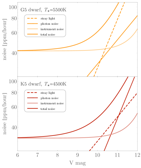
Figure 1: Illustration of the noise model adopted in this work for CHEOPS, showing the different noise components affecting the total. We linearly interpolate the G5 and K5 total noise models as a function of effective temperature, except for temperatures exceeding these two extremes, beyond which we simply adopt the nearest neighbor model.

Because of the specific bandpass of the mission, stars of different temperature will have distinct noise curves and thus we were provided with noise estimates for a 4500 K K5-dwarf and a 5500 K G5-dwarf, as a point of comparison. Although we do not have a bandpass available, we can estimate the noise at intermediate temperatures between these two extremes by simply linearly interpolating between the two, as a first-order approximation. For stars cooler than 4500 K, we simply adopt the K5 values and similarly for stars hotter than 5500 K the G5 model is assumed.

With the noise in hand, one may now easily calculate the SNR over one hour of cumulative integration time, a term we write as $\mathrm{SNR}_{\mathrm{hour}}$. For each target, we make this calculation on a posterior sample-by-sample basis allowing us to predict a posterior for $\mathrm{SNR}_{\mathrm{hour}}$ and thus the credible intervals, which are reported later in Table 1.

It is important to stress that that our one-hour cumulative SNR does not make any assumptions about how the one hour of integration time is achieved (e.g. combining multiple orbits or epochs). In practice, the orbit of CHEOPS will lead to observing gaps and thus one hour of wall time will not equal one hour of cumulative integration time, unless the target happens to lie within a continuous viewing zone. We therefore stress that observers will need to account for the observational duty cycle, $\mathcal{D}$ (based on orbital viewing and scheduling constraints), the number of transit epochs observed, $N$, and transit duration, $\tilde{T}$, and the amount of out-of-transit data acquired, $B$. Accordingly, the actual SNR will follow

$$\mathrm{SNR} =\sqrt{\sum_{i=1}^{N}\mathrm{SNR}_{\mathrm{hour}}^{2}\Big{(}\frac{\mathcal{D}_{i}\tilde{T}B_{i}}{B_{i}+\tilde{T}}\Big{)}},$$ (6)

where $\tilde{T}$ is the 1.5-to-3.5 contact transit duration defined in Kipping (2010), $\mathcal{D}_{i}$ and $B_{i}$ are the duty cycle and out-of-transit baseline of the $i^{\mathrm{th}}$ transit epoch observed, amongst $N$ transits. Equation 6 comes from Equation 9 of Kipping & Sandford (2016), and assuming $W\delta\ll T_{14}$, where $W\equiv(T_{14}+T_{23})/2$ and $T_{14}$ and $T_{23}$ are the first-to-fourth and second-to-third contact duration. Equation 6 also assumes that $T_{14}\simeq W\simeq\tilde{T}$ for the sake of simplicity.

Of course, without a detailed orbital model or list of scheduling requirements imposed by other programs, it is not generally possible at this stage for us to estimate all of the above parameters in advance. However, we do calculate a one-sigma credible interval for $\tilde{T}$ in the optimistic limit of an equatorial transit, accounting for the known eccentricity of the planet using Equation 15 of Kipping (2010), which is provided later in Table 1. Nevertheless, our provision of $\mathrm{SNR}_{\mathrm{hour}}$ offers a straight-forward means for the community to estimate and rank planets by their detectability under various circumstances.

2.8 Transit probabilities

In what has been described so far, we have computed the probability distribution of the $\mathrm{SNR}_{\mathrm{hour}}$ of each RV planet as observed by one integrated hour of CHEOPS telescope time, conditioned upon the assumption that a planet transits. This may be broadly described as computing the detectability, the primary goal of this work, but not the actual yield. The actual yield will be affected by which planets are observed and for how long, the observing strategy and cadence, and the a-priori transit probability of each planet. Since the observing strategy for CHEOPS has not yet been decided upon and will likely evolve during the mission, it is generally not possible to model the yield at this time. Instead, for context, we compute here the a-priori transit probability of each planet.

Finally, for each predicted transit depth, we estimate the geometric transit probability. This calculation is done in the simple case of assuming an isotropic inclination prior, although we note that the true distribution is likely more favorable than this but requires detailed modeling of the mass functions (Stevens & Gaudi, 2013). Also, we do not estimate a credible interval for the transit probabilities, rather simply adopt the maximum a-posteriori system parameters to compute a single point-estimate for each planet. This is largely motivated by the lack of publicly available joint posteriors on eccentricity and argument of periastron, necessary for such a calculation. Since our $\mathrm{SNR}_{\mathrm{hour}}$ posteriors are conditioned upon the assumption of a transit, these unknown covariances do not propagate into our earlier $\mathrm{SNR}_{\mathrm{hour}}$ calculations fortunately.

In calculating the transit probability, we account for the effects of orbital eccentricity, $e$ and argument of periapsis, $\omega$, by using (Barnes, 2007; Burke, 2008):

$$\mathrm{Pr}(\mathrm{transit})=\Bigg{(}\frac{R_{\star}}{a}\Bigg{)}\Bigg{(}\frac{1+e\sin\omega}{1-e^{2}}\Bigg{)}.$$ (7)

In some cases, the eccentricity or argument of periastron was not available on EOD, in which case simply assume a circular orbit for simplicity. In cases where $(a/R_{\star})$ was not available, we quote the transit probability as “N/A”, rather than completely dropping them from our list.

3 Detectable Planets with CHEOPS

3.1 Overview of results

After predicting posterior distributions for $R_{P}$, $\delta$ and $\mathrm{SNR}_{\mathrm{hour}}$ as described earlier, we tabulated the medians, as well as the 68.3% and 95.5% credible intervals in Table 1. To illustrate a specific example, we show a corner plot of the posteriors produced in this work for the planet HD 20794c in Figure 2, which highlights the covariances, even between mass and radius owing to HD 20794c’s location near the Terran-Neptunian divide.

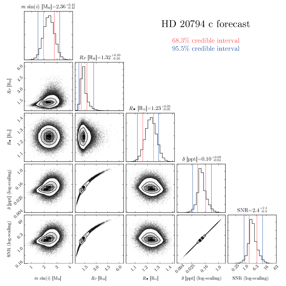
Figure 2: Corner plot of our resulting posteriors for HD 20794c an illustrative example. Covariances are evident between the parameters, including between mass and radius.

Table 1: Final predicted properties for 468 RV planets using forecaster. Only a portion of the table is shown here, the full version is available in the online version and at this URL. SNR values correspond to one cumulative hour of integration time.

Name	$m$ $[M_{\oplus}]$	$R_{P}$ $[R_{\oplus}]$	$\delta=(R_{P}/R_{\star})^{2}$ [ppt]	$\mathrm{SNR}_{\mathrm{hour}}$	$\tilde{T}_{\mathrm{max}}$ [hours]	$\mathrm{P}(\mathrm{transit})$
Alp Cen B b	$1.127\pm 0.096$	$[0.82,0.93,1.04,1.16,1.34]$	$[0.07,0.09,0.11,0.14,0.19]$	$[1.7,2.2,2.8,3.6,4.8]$	$2.42_{-0.08}^{+0.08}$	10.1%
GJ 581 e	$1.95\pm 0.22$	$[0.75,1.04,1.23,1.45,2.24]$	$[0.5,1.0,1.4,2.1,4.7]$	$[8,17,23,35,78]$	$1.19_{-0.05}^{+0.05}$	4.0%
HD 20794 c	$2.36\pm 0.43$	$[0.75,1.06,1.32,1.81,2.69]$	$[0.03,0.06,0.10,0.18,0.41]$	$[0.8,1.5,2.4,4.5,10.0]$	$8.2_{-0.3}^{+0.4}$	2.8%
HD 20794 b	$2.70\pm 0.31$	$[0.76,1.09,1.42,1.99,2.88]$	$[0.03,0.07,0.11,0.22,0.47]$	$[0.8,1.6,2.8,5.4,11.5]$	$6.3_{-0.3}^{+0.3}$	4.7%
HD 85512 b	$3.62\pm 0.44$	$[0.85,1.22,1.70,2.42,3.46]$	$[0.08,0.16,0.32,0.65,1.37]$	$[2.1,4.5,8.9,18.4,38.5]$	$6.4_{-0.7}^{+0.7}$	1.6%
$\vdots$	$\vdots$	$\vdots$	$\vdots$	$\vdots$	$\vdots$	$\vdots$

For each planet, we also recorded the most probable classification outputted from forecaster (Terran, Neptunian, Jovian or Stellar). Amongst the 468 RV planets studied, we find zero instances of a Stellar classification, which is to be expected, 354 Jovians, 112 Neptunians and 2 Terrans (Alpha Centauri A b and GJ 581 e). Amongst the Neptunian worlds, we split them into groups based by dividing about 10 $M_{\oplus}$ in terms of maximum a-posteriori reported mass on EOD, defining a subset of mini-Neptunes (28 planets) and Neptunes (84 planets).

In Figure 3, we show three histograms for each type of planet’s maximum a-posteriori forecasted $\mathrm{SNR}_{\mathrm{hour}}$. Given that even short-period planetary transits typically last for a couple of hours, the high $\mathrm{SNR}_{\mathrm{hour}}$ values seen in Figure 3 imply that the vast majority of these RV planets are expected to be detectable with CHEOPS with a single event. Specifically, we find a maximum a-posteriori $\mathrm{SNR}_{\mathrm{hour}}$ exceeding 10 for 22 of the 28 mini-Neptunes, 82 of the 84 Neptunes and 294 of 354 Jovians. However, we highlight that our $\mathrm{SNR}_{\mathrm{hour}}$ calculations assume no intrinsic photometric noise for the parent stars, which may in some case significantly affect the estimates given (discussed further in Section 4).

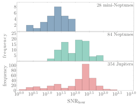
Figure 3: Histograms of the $\mathrm{SNR}_{\mathrm{hour}}$ (in log space) for the three broad class of planets considered in this work. The majority of the RV planets would be detectable in transit using CHEOPS with a single transit observation, assuming the stars are not highly active.

For the two Terrans, GJ 581 e is expected to be easily detectable (assuming it transits) at $\mathrm{SNR}_{\mathrm{hour}}\sim$20 but Alpha Cen B b would be more challenging at $\mathrm{SNR}_{\mathrm{hour}}$ of a few, requiring likely more than a single transit observation. However, we point out that transits of both of these high-profile planets has already been investigated, with transits generally excluded for both (Dragomir et al., 2012; Demory et al., 2015).

3.2 CHEOPS vs Kepler planets

CHEOPS is not a wide-field transit survey and thus should not be expected to find remotely near as many planets as that discovered by Kepler. However, transiting planets discovered by CHEOPS have the potential to be significantly brighter than those of Kepler, an argument which originally motivated the CHEOPS project (Broeg et al., 2013). To investigate this, Figure 4 shows the apparent magnitude (treating $V$-band and the Kepler bandpass as being approximately equal) of the Kepler planets as a function of their size, versus the RV planets, where $\mathrm{SNR}_{\mathrm{hour}}$ is computed as described in Section 2.7.

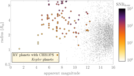
Figure 4: Radii of the Kepler planets (gray) as function of their apparent magnitude. For comparison, we show the RV planets where the $\mathrm{SNR}_{\mathrm{hour}}$ is provided using the colour scale, assuming the CHEOPS-like SNRs derived in this work. As expected, CHEOPS indeed has the capability to provide transiting planets orbiting far brighter stars than that of Kepler.

Figure 4 confirms that if CHEOPS targets the bright RV planets, it should be expected to deliver a subset of significantly brighter transiting planets than those found by Kepler. However, we also stress that the planet yield will almost certainly be far smaller, and the smallest possible detectable planet will be larger than the smaller Kepler worlds, owing to the fact RV detections do not currently probe into the sub-Earth mass regime reliably.

3.3 Validating the predictions

The forecaster model from Chen & Kipping (2017a) has been subject to extensive testing, particularly in the original paper but also that of Chen & Kipping (2017b). Nevertheless, to validate our predictions we subject to it another test by extracting the RV planets in our sample for which the planetary radius has been directly measured via a transit detection.

There are only nine such cases in our sample (HD 189733b, HD 209458b, HD 80606b, GJ 436b, GJ 3470b, HD 17156b, HD 149026b, HD 97658b, 55 Cnc e). We compare the predictions versus the observations in Figure 5, which reveals that our predictions are fully compatible with the observed values. Only one of our predicted radii falls outside of the 1 $\sigma$ credible interval (HD 149026b), yet this object falls within the 2 $\sigma$ prediction. This is not statistically surprising, since amongst a sample of nine objects it should not be generally expected that all nine fall within a 68.3% probability interval.

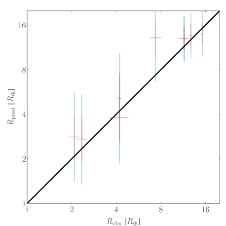
Figure 5: A comparison of predicted planetary radii from this work using the forecaster package of Chen & Kipping (2017a) and reported measured planetary radii. Only nine planets in our sample have a measured radius from transits. Blue denotes the 2 $\sigma$ confidence region and red the 1 $\sigma$.

4 Discussion

In this work, we have predicted the planetary radii, transit depths and associated signal-to-noises (SNRs) using CHEOPS (Broeg et al., 2013) for 468 planets listed on the “Exoplanet Orbit Database” (EOD; Han et al. 2014) as having been discovered using the radial velocity (RV) method. Our SNR values assume one-hour of cumulative integration time, no intrinsic stellar noise, employ a CHEOPS noise model dependent on spectral type and apparent magnitude, and accounts for instrument saturation. This fiducial choice of a one-hour integration time is a general value which may be easily transformed to account for the number of transits observed, the observational duty cycle of each transit (e.g. due to CHEOPS’ orbit) and the (unknown) transit duration (see Equation 6). Predictions for planetary radii are based using the empirical, probabilistic framework known as forecaster presented by Chen & Kipping (2017a).

We have verified that our predictions are consistent with the observed planetary radii in nine cases where the RV planets have been established to transit. Amongst the other planets, we predict that CHEOPS will be able to detect transits at $\mathrm{SNR}_{\mathrm{hour}}>10$ for the vast majority, assuming that they have the correct geometry and our assumptions hold true. The greatest unknown quantity in our model is the potential for intrinsic photometric variability of the parent stars, which in optical bandpasses has been demonstrably shown to a major impediment to transit discovery if present (Kipping et al., 2017). For this reason, it may be worthwhile for CHEOPS to conduct preliminary photometric observations of planned targets during quiet times, in order to ascertain the possibility of activity.

Using the classifications made by forecaster, we predict that only two of the RV planets considered are most likely Terran (Alpha Cen A b and GJ 581 e), yet both have already been established to be unlikely to transit (Dragomir et al., 2012; Demory et al., 2015). Amongst the 92 mini-Neptunes and 20 Neptune-sized planets, we find typical transit probabilities of order 5% and thus predict numerous discoveries from CHEOPS with a suitable observing strategy.

The main objective of this work is to aid the CHEOPS team in predicting which RV planets are most suitable for follow-up efforts in a quantifiable manner. Aside from pursuing RV planets, we highlight that it may also be fruitful to target known planetary systems where additional planets are confidently predicted using machine learning methods, such as that presented in Kipping & Lam (2017). Undoubtedly targets-of-opportunity will arise before the expected launch in 2018, yet a library of pre-computed forecasted SNRs should aid the team in scheduling observations amongst these other opportunities. Whilst this work has certainly had CHEOPS directly in mind due to the unique strategy planned, the predictions for the transit depths are not specific to CHEOPS and thus may also benefit other transit surveys.

Our predictions establish that CHEOPS should find transiting planets orbiting far brighter target stars than that of Kepler. For example, amongst the 104 Neptunian RV planets with satisfying $\mathrm{SNR}_{\mathrm{hour}}>10$, 86 of them will be orbiting stars brighter than $V=10$, providing exciting opportunities for atmospheric characterization both from the ground and space. To aid the community in planning both the CHEOPS observing strategy and potential follow-up, we make our predictions publicly available at this URL.

References

- Akeson et al. (2013) Akeson, R. L., Chen, X., Ciardi, D., et al. 2013, PASP, 125, 989
- Bakos et al. (2004) Bakos, G. Á., Noyes, R. W., Kovács, G., Stanek, K. Z., Sasselov, D. D. & Domsa, I. 2004, PASP, 116, 266
- Bakos et al. (2013) Bakos, G. Á., Csubry, Z., Penev, K., et al. 2013, PASP, 125, 154
- Barnes (2007) Barnes, J. W. 2007, PASP, 119, 986
- Batygin & Stevenson (2013) Batygin, K. & Stevenson, D. J. 2013, ApJ, 769, L9
- Broeg et al. (2013) Broeg, C., Fortier, A., Ehrenreich, D., et al. 2013, EPJ Web Conf., 47, 3005
- Burke (2008) Burke, C. J. 2008, ApJ, 679, 1566
- Burke et al. (2015) Burke, C. J., Christiansen, J. L., Mullally, F., et al. 2015, ApJ, 809, 8
- Charbonneau et al. (2009) Charbonneau, D., Berta, Z. K., Irwin, J., et al. 2009, Nature, 462, 891
- Chen & Kipping (2017a) Chen, J. & Kipping, D. M. 2017, ApJ 834, 17
- Chen & Kipping (2017b) Chen, J. & Kipping, D. M. 2017, MNRAS, submitted (arXiv e-prints:1706.01522)
- Coughlin et al. (2016) Coughlin, J. L., Mullally, F., Thompson, S. E., et al. 2016, ApJS, 224, 12
- Demory et al. (2015) Demory, B.-O., Ehrenreich, D., Queloz, D., et al. 2015, MNRAS, 450, 2043
- Dragomir et al. (2012) Dragomir, D., Matthews, J. M., Kuschnig, R., et al. 2012, ApJ, 759, 2
- Dragomir et al. (2013) Dragomir, D., Matthews, J. M., Eastman, J. D., et al. 2013, ApJ, 772, 2
- Doyle et al. (2011) Doyle, L. R., Carter, J. A., Fabrycky, D. C., et al. 2011, Science, 333, 1602
- Dressing & Charbonneau (2015) Dressing, C. D. & Charbonneau, D. 2015, ApJ, 807, 45
- Han et al. (2014) Han, E., Wang, S. X., Wright, J. T., Feng, Y. K., Zhao, M., Fakhouri, O., Brown, J. I. & Hancock, C. 2014, PASP, 126, 827
- Hou et al. (2014) Hou, F., Goodman, J. & Hogg, D. W. 2014, arXiv e-prints:1401.6128
- Howard et al. (2012) Howard, A. W., Marcy, G. W., Bryson, S. T., et al. 2012, ApJS, 201, 15
- Ford (2006) Ford, E. B. 2006, ApJ, 642, 505
- Fortney et al. (2011) Fortney, J. J. & Nettelmann, N. 2010, Space Sci. Rev., 152, 423
- Irwin et al. (2015) Irwin, J. M., Berta-Thompson, Z. K., Charbonneau, D., Dittmann, J., Falco, E. E., Newton, E. R. & Nutzman P. 2015, in van Belle, G. T., Harris, H. C., eds, 18th Cambridge Workshop on Cool Stars, Stellar Systems, and the Sun. Astron. Soc. Pac., San Francisco, p. 767
- Kipping (2010) Kipping, D. M. 2010, MNRAS, 407, 301
- Kipping & Sandford (2016) Kipping, D. M. & Sandford, E. 2016, MNRAS, 463, 1323
- Kipping & Lam (2017) Kipping, D. M. & Lam, C. 2017, MNRAS, 465, 3495
- Kipping et al. (2017) Kipping, D. M., Cameron, C., Hartman, J. D., et al. 2017, AJ, 153, 93
- Lissauer et al. (2012) Lissauer, J. J., Fabrycky, D. C., Ford, E. B., et al. 2011, Nature, 470, 53
- Pollacco et al. (2006) Pollacco, D. L., Skillen, I., Collier Cameron, A., et al. 2006, PASP, 118, 1407
- Rauer et al. (2014) Rauer, H., Catala, C., Aerts, C., et al. 2014, Exp. Astron., 38, 249
- Ricker et al. (2015) Ricker G. R., Winn, J. N., Vanderspeck, R., et al. 2015, J. Astron. Telescopes, Instrum. Syst., 1, 014003
- Rucinski et al. (2003) Rucinski, S., Carroll, K., Kuschnig, R., Matthews, J. M., & Stibrany, P. 2003, Adv. Space Res., 31, 371
- Seager et al. (2007) Seager, S., Kuchner, M., Hier-Majumder, C. A. & Militzer, B. 2007, ApJ, 669, 1279
- Stevens & Gaudi (2013) Stevens, D. J. & Gaudi, S. B. 2013, PASP, 125, 933
- Tuomi et al. (2012) Tuomi, M. 2012, A&A, 543, 52
- Wheatley et al. (2013) Wheatley, P. J., Pollacco, D. L., Queloz, D., et al. 2013, EPJ Web Conf., 47, 13002
- Wilson et al. (2008) Wilson, D. M., Gillon, M., Hellier, C., et al. 2008, ApJ, 675, 113
- Winn et al. (2011) Winn, J. N., Matthews, J. M., Dawson, R. I., et al. 2011, ApJ, 737, 18
- Wolfgang et al. (2016) Wolfgang, A., Rogers, L. A. & Ford, E. B. 2016, ApJ, 825, 19