Light-weight pixel context encoders for image inpainting

Abstract.

In this work we propose Pixel Content Encoders (PCE), a light-weight image inpainting model, capable of generating novel content for large missing regions in images. Unlike previously presented convolutional neural network based models, our PCE model has an order of magnitude fewer trainable parameters. Moreover, by incorporating dilated convolutions we are able to preserve fine grained spatial information, achieving state-of-the-art performance on benchmark datasets of natural images and paintings. Besides image inpainting, we show that without changing the architecture, PCE can be used for image extrapolation, generating novel content beyond existing image boundaries.

1. Introduction

Reconstructing missing or damaged regions of paintings has long required a skilled conservator or artist. Retouching or inpainting is typically only done for small regions, for instance to hide small defects (Bertalmio et al., 2000). Inpainting a larger region requires connoisseurship and imagination: the context provides clues as to how the missing region might have looked, but generally there is no definitive evidence. Therefore, sometimes the choice is made to inpaint in a conservative manner. Take for example the painting in Figure 1, the left bottom corner was filled with a ‘neutral’ colour as to not change the interpretation of the artwork. However, with the emergence of powerful computer vision methods specialising in inpainting (Chan et al., 2011; Cornelis et al., 2013; Pathak et al., 2016; Iizuka et al., 2017), it has become possible to explore what a potential inpainting result might look like, without physically changing the painting.

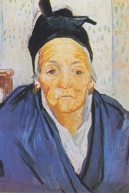
Figure 1. “An old woman of Arles” by Vincent van Gogh (courtesy of the Van Gogh Museum). The left bottom corner was manually inpainted with a ‘neutral’ colour.

Although image inpainting algorithms are not a novel development (Bertalmio et al., 2000; Barnes et al., 2009), recent work has shown that approaches based on Convolutional Neural Networks (CNN) are capable of inpainting large missing image regions in a manner which is consistent with the context (Pathak et al., 2016; Yeh et al., 2016; Yang et al., 2017; Iizuka et al., 2017). Unlike, scene-completion approaches (Hays and Efros, 2007), which search for similar patches in a large database of images, CNN-based approaches are capable of generating meaningful content (Pathak et al., 2016).

A key aspect of CNN-based inpainting approaches and of many CNN architectures in general (Sermanet and Lecun, 2011), is that an image is described at multiple scales by an encoder that reduces the spatial resolution through pooling and downsampling. Each layer (or block of layers) of the network processes the image at a certain scale, and passes this scale-specific information on to the next layer. This encoding process continues until a single low dimensional representation of the image is found, which describes the entire image. Because this architecture resembles a funnel, the final representation is sometimes referred to as the bottleneck. Figure 2 shows a visualisation of two CNN architectures; one for classification, and one for image generation (similar to an autoencoder). Both architectures encode the image into a bottleneck representation, after which the classification network processes it with a classifier, typically a softmax regression layer (Krizhevsky et al., 2012), and the image generation network feeds it to a decoder (Isola et al., 2016). The decoder subsequently performs a number of upsampling steps to generate the output image.

Figure 2. Visualisation of a classification CNN architecture (left), and an image generation architecture (right). In both architectures the encoder downsamples the input into a low(er) dimensional representation: the bottleneck.

A downside of downsampling in the encoder is the loss of spatial detail - detail which might be crucial to the task (Yu et al., 2017). For inpainting this is most prevalent when considering the local consistency (Iizuka et al., 2017); the consistency between the edge of the inpainted region and the edge of the context. A lack of local consistency will result in an obvious transition from the context to the inpainted region. Although increasing the size of the bottleneck, i.e., making it wider, appears to alleviate this to some extent (Pathak et al., 2016), it comes at the cost of a tremendous increase in model parameters. Luckily, recent work has shown that it is possible to encode an image while preserving the spatial resolution (Yu and Koltun, 2016; Yu et al., 2017). Dilated convolutions make it possible to expand the receptive field of a CNN, without downsampling or increasing the number of model parameters. We define the receptive field of a CNN as the size of the region in the input space that affect the output neurons of the encoder. For instance, a single layer CNN with $3\times 3$ filters would have a receptive field of $3\times 3$, adding identical layers on top would increase the receptive field to $5\times 5$, $7\times 7$, etc. We refer to Section 2.2 for an explanation of how the receptive field of a CNN grows when using dilated convolutions.

Many of the shown results obtained with CNN-based inpainting models, have been achieved using complex architectures with many parameters, resulting in a necessity of large amounts of data, and often long training times (Pathak et al., 2016; Iizuka et al., 2017). Although simpler architectures have been proposed (Yeh et al., 2016), these are typically only demonstrated on small datasets with relatively little variation (i.e., only faces or only facades of buildings). Therefore, we aim to produce a light-weight inpainting model, which can be applied to large and complex datasets. In this paper, we demonstrate that using dilated convolutions we can construct a simple model that is able to obtain state-of-the-art performance on various inpainting tasks.

The remainder of this paper is organised as follows. In Section 2 we discuss related work on inpainting and dilated convolutions. In 3 we describe the architecture of our model and how it is trained. Section 4 describes the experiments and the results we obtain on a variety of inpainting tasks. Lastly, in Section 5 we conclude that our model is much less complex than existing models, while outperforming them on benchmark datasets of natural images and paintings.

2. Related work

In this section we will discuss work related to image inpainting, dilated convolutions and their application to inpainting, and finally our contributions.

2.1. Image inpainting

When a single pixel is missing from an image we can look at the adjacent pixels and average their colour values to produce a reasonable reconstruction of the missing pixel. When a larger region formed by directly adjacent pixels is missing, it is necessary to take into account a larger neighbourhood surrounding the missing region. Moreover, it may become insufficient to only smooth out the colour, to reconstruct the region in a plausible manner. Additionally, for smaller regions it can be sufficient to only incorporate textural or structural information (Bertalmio et al., 2003), however inpainting larger regions requires understanding of the entire scene (Pathak et al., 2016). For example, given a picture of a face, if part of the nose is missing it can be reconstructed by looking at the local context and textures. But once the entire nose is missing it requires understanding of the entire face to be able to reconstruct the nose, rather than smooth skin (Yeh et al., 2016).

The challenge of inferring (large) missing parts of images is at the core of image inpainting, the process of reconstructing missing or damaged parts of images (Bertalmio et al., 2000).

Classical inpainting approaches typically focus on using the local context to reconstruct smaller regions, in this paper we will focus on recent work using Convolutional Neural Networks (CNN) to encode the information in the entire and inpaint large regions (Pathak et al., 2016; Yeh et al., 2016; Yang et al., 2017; Gao and Grauman, 2017; Iizuka et al., 2017). From these recent works we will focus on two works, first the work by Pathak et al. (Pathak et al., 2016) who designed the (until now) ‘canonical’ way of performing inpainting with CNN. Second, we will focus on the work by Iizuka et al. (Iizuka et al., 2017), who very recently proposed several extensions of the work by Pathak et al., including incorporating dilated convolutions.

Pathak et al. (Pathak et al., 2016) present Context Encoders (CEs), a CNN trained to inpaint while conditioned on the context of the missing region. CE describe the context of the missing region by encoding the entire image into a bottleneck representation. Specifically, the spatial resolution of the input image is reduced with a factor $128$; from $128\times 128$, to the bottleneck representation - a single vector. To compensate for the loss of spatial resolution they increase the width of the bottleneck to be $4000$ dimensional. Notably, this increases the total number of model parameters tremendously, as compared to a narrower bottleneck.

CEs are trained by means of a reconstruction loss (L2), and an adversarial loss. The adversarial loss is based on Generative Adversarial Networks (GAN) (Goodfellow et al., 2014), which involves training a discriminator $D$ to distinguish between real and fake examples. The real examples are samples from the data $x$, whereas the fake examples are produced by the generator $G$. Formally the GAN loss is defined as:

(1) $$\min_{G}\max_{D}\mathbb{E}_{x\sim p_{data}(x)}[log(D(x)+log(1-D(G(x))]$$

by minimising this loss the generator can be optimised to produce examples which are indistinguishable from real examples. In (Pathak et al., 2016) the generator is defined as the CE, and the discriminator is a CNN trained to distinguish original images from inpainted images.

In a more recent paper, Iizuka et al. (Iizuka et al., 2017) propose two extensions to the work by Pathak et al. (Pathak et al., 2016): (1) They reduce the amount of downsampling by incorporating dilated convolutions, and only downsample by a factor $4$, in contrast to Pathak et al. who downsample by a factor $128$. (2) They argue that in order to obtain globally and locally coherent inpainting results, it is necessary to extend the GAN framework used in (Pathak et al., 2016) by using two discriminators. A ‘local’ discriminator which focuses on a small region centred around the inpainted region, and a ‘global’ discriminator which is trained on the entire image. Although the qualitative results presented in (Iizuka et al., 2017) appear intuitive and convincing, the introduction of a second discriminator results in a large increase in the number of trainable parameters.

Ablation studies presented in a number of works on inpainting have shown that the structural (e.g., L1 or L2) loss results in blurry images (Pathak et al., 2016; Yang et al., 2017; Iizuka et al., 2017). Nonetheless, these blurry images do accurately capture the coarse structure, i.e., the low spatial frequencies. This matches an observation by Isola et al. (Isola et al., 2016), who stated that if the structural loss captures the low spatial frequencies, the GAN loss can be tailored to focus on the high spatial frequencies (the details). Specifically, Isola et al. introduced PatchGAN, a GAN which focuses on the structure in local patches, relying on the structural loss to ensure correctness of the global structure. PatchGAN, produces a judgement for $N\times N$ patches, where $N$ can be much smaller than the whole image. When $N$ is smaller than the image, PatchGAN is applied convolutionally and the judgements are averaged to produce a single outcome.

Because the PatchGAN operates on patches it has to downsample less, reducing the number of parameters as compared to typical GAN architectures, this fits well with our aim to produce a light-weight inpainting model. Therefore, in our work we choose to use the PatchGAN for all experiments.

Before turning to explanation of the complete model in section 3, we first describe dilated convolutions in more detail.

2.2. Dilated convolutions

The convolutional layers of most CNN architectures use discrete convolutions. In discrete convolutions a pixel in the output is the sum of the elementwise multiplication between the weights in the filter and a region of adjacent pixels in the input. Dilated or $l$-dilated convolutions offer a generalisation of discrete convolutions (Yu and Koltun, 2016) by introducing a dilation factor $l$ which determines the ‘sampling’ distance between pixels in the input. For $l=1$, dilated convolutions correspond to discrete convolutions. By increasing the dilation factor, the distance between pixels sampled from the input becomes larger. This results in an increase in the size of the receptive field, without increasing the number of weights in the filter. Figure 3 provides a visual illustration of dilated convolution filters.

(a)

(b)

(c)

Figure 3. Comparison of $1$-dilated versus $2$-dilated filter. (a) shows the receptive field of a $3\times 3$ $1$-dilated filter directly on the input. (b) shows the $5\times 5$ receptive field of a $1$-dilated $3\times 3$ filter applied to (a). (c) shows the $7\times 7$ receptive field of a $2$-dilated $3\times 3$ filter applied to (a). (c) has a larger receptive field than (b), with the same number of parameters.

Recent work has demonstrated that architectures using dilated convolutions are especially promising for image analysis tasks requiring detailed understanding of the scene (Yu and Koltun, 2016; Yu et al., 2017; Iizuka et al., 2017). For inpainting the aim is to fill the missing region in a manner which is both globally and locally coherent, therefore it relies strongly on a detailed scene understanding. In this work we incorporate lessons learnt from the work by Yu et al. (Yu and Koltun, 2016; Yu et al., 2017) and Iizuka et al. (Iizuka et al., 2017) and present a lightweight and flexible inpainting model with minimal downsampling.

2.3. Our contributions

In this work we make the following four contributions. (1) We present a light-weight and flexible inpainting model, with an order of magnitude fewer parameters than used in previous work. (2) We show state-of-the-art inpainting performance on datasets of natural images and paintings. (3) While acknowledging that a number of works have explored inpainting of cracks in paintings (Giakoumis et al., 2006; Solanki and Mahajan, 2009; Cornelis et al., 2013), we pose that we are the first to explore inpaintings of large regions of paintings. (4) We demonstrate that our model is capable of extending images (i.e., image extrapolation), by generating novel content which extends beyond the edges of the current image.

3. Pixel Context Encoders

In this section we will describe our inpainting model: Pixel Context Encoders (PCE). Firstly, we will describe the PCE architecture, followed by details on the loss function used for training.

3.1. Architecture

Typically, Convolutional Neural Networks which are used for image generation follow an encoder-decoder type architecture (Isola et al., 2016). The encoder compresses the input, and the decoder uses the compressed representation (i.e., the bottleneck) to generate the output. Our PCE does not have a bottleneck, nevertheless we do distinguish between a block of layers which encodes the context (the encoder), and a block of layers which take the encoding of the image and produces the output image, with the missing region filled in (the decoder).

Figure 4. Visualisation of the PCE architecture. Unlike traditional encoder-decoder architectures, the PCE architecture does not have a bottleneck. The encoder describes the context (i.e., the input), and the decoder generates the output image.

The encoder consists of two downsampling layers, followed by a block of $n$ dilated convolutional layers. The downsampling layers of the encoder are discrete convolutions with a stride of $2$. For the subsequent dilated convolution layers, the dilation rate $d$ increases exponentially. The depth of the encoder is chosen such that the receptive field of the encoder is (at least) larger than the missing region, for all of our experiments $n=4$, resulting in a receptive field of $247\times 247$. Table 1 shows how the size of the receptive field grows as more layers are added to the encoder.

By incorporating strided convolutions in the first two layers we follow Iizuka et al. (Iizuka et al., 2017) and downsample the images by a factor $4$, our empirical results showed that this improves inpainting performance and drastically reduces ($5$ to $6$ times) memory requirements as compared to no downsampling. We pose that the increased performance stems from the larger receptive field, and the local redundancy of images, i.e., neighbouring pixels tend to be very similar. Nonetheless, we expect that stronger downsampling will results in too great of a loss of spatial resolution, lowering the inpainting performance.

Table 1. Growth of the PCE receptive field (RF) and dilation rate $d$ as a function of the number of layers (depth), with a filter size of $3\times 3$. The first two layers are discrete convolutions with a stride of $2$.

Depth	$d$	RF size
$1$	$1$	$3\times 3$
$2$	$1$	$7\times 7$
$3$	$2$	$23\times 23$
$4$	$4$	$55\times 55$
$5$	$8$	$119\times 119$
$6$	$16$	$247\times 247$

The decoder consists of a block of $3$ discrete convolutional layers which take as input the image encoding produced by the encoder. The last two layers of the decoder are preceded by a nearest-neighbour interpolation layer, which upsamples by a factor $2$, restoring the image to the original resolution. Additionally, the last layer maps the image encoding back to RGB space (i.e., $3$ colour channels), after which all pixels which were not missing are restored to the ground-truth values.

All convolutional layers in the encoder and decoder, except for the last decoder layer, are followed by a Batch Normalisation layer (Ioffe and Szegedy, 2015). The activation functions for all convolutional layers in the encoder and decoder are Exponential Linear Units (ELU) (Clevert et al., 2016).

3.2. Loss

PCEs are trained through self-supervision; an image is artificially corrupted, and the model is trained to regress back the uncorrupted ground-truth content. The PCE $F$ takes an image $x$ and a binary mask $M$ (the binary mask $M$ is one for masked pixels, and zero for the pixels which are provided) and aims to generate plausible content for the masked content $F(x,M)$. During training we rely on two loss functions to optimise the network: a L1 loss and a GAN loss. For the GAN loss we specifically use the PatchGAN discriminator introduced by Isola et al. (Isola et al., 2016).

The L1 loss is masked such that the loss is only non-zero inside the corrupted region:

(2) $$\mathcal{L}_{L1}=\lVert M\odot(F(x,M)-x)\rVert_{1}$$

where $\odot$ is the element-wise multiplication operation.

Generally, the PatchGAN loss is defined as follows:

(3) $$\min_{G}\max_{D}\mathbb{E}_{x\sim p_{data}(x)}[log(D(x)+log(1-D(G(x))]$$

where the discriminator $D$ aims to distinguish real from fake samples, and the generator $G$ aims to fool the discriminator. For our task we adapt the loss to use our PCE as the generator:

(4) $$\begin{split}\mathcal{L}_{GAN}=\min_{F}\max_{D}\mathbb{E}_{x\sim p_{data}(x)}[log(D(x)+\\ log(1-D(F(x,M))],\end{split}$$

our discriminator is similar to the global discriminator used in (Iizuka et al., 2017), except that we restore the ground-truth pixels before processing the generated image with the discriminator. This allows the discriminator to focus on ensuring that the generated region is consistent with the context.

The overal loss used for training thus becomes:

(5) $$\mathcal{L}=\lambda\mathcal{L}_{L1}+(1-\lambda)\mathcal{L}_{GAN}$$

where $\lambda$ is fixed at $0.999$ for all experiments, following (Pathak et al., 2016).

4. Experiments

To evaluate the performance of our PCE we test it on a number of datasets and variations of the inpainting task. In this section we will describe the datasets and the experimental setting used for training, the results of image inpainting on $128\times 128$ and $256\times 256$ images, and lastly the image extrapolation results.

All results are reported using the Root Mean Square Error (RMSE) and Peak Signal Noise Ratio (PSNR) between the uncorrupted ground truth and the output produced by the models.

4.1. Datasets

ImageNet. As a set of natural images we use the subset of $100,000$ images that Pathak et al. (Pathak et al., 2016) selected from the ImageNet dataset (Russakovsky et al., 2014). The performance is reported on the complete ImageNet validation set consisting of $50,000$ images.

PaintersN. The “Painters by Numbers” dataset (PaintersN) as published on Kaggle consists of $103,250$ photographic reproductions of artworks by well over a thousand different artists. The dataset is divided into a training set ($93,250$ images), validation set ($5000$ images), and test set ($5000$ images) used for training the model, optimising hyper-parameters, and reporting performances, respectively.

For both datasets all images were scaled such that the shortest side was $256$ pixels, and then a randomly located $256\times 256$ crop was extracted.

4.2. Experimental settings

In this section the details on the settings of the hyperparameters and training procedure are provided. The layers of the encoder and the decoder consist of $128$ filters with spatial dimensions of $3\times 3$ for all experiments in this work. All dilated layers were initialised using identity initialisation cf. (Yu and Koltun, 2016), which sets the weights in the filter such that initially each layer simply passes its input to the next. All discrete convolutional layers were initialised using Xavier initialisation (Glorot and Bengio, 2010).

The PatchGAN discriminator we used consists of $5$ layers of filters with spatial dimensions of $3\times 3$, using LeakyReLU as the activation function ($\alpha=0.2$). For the first $4$ layers the number of filters increases exponentially (i.e., $64$, $128$, $256$, $512$), the 5th layer outputs a single channel, the real/fake judgement for each patch in the input.

The network was optimised using ADAM (Kingma and Ba, 2015) until the L1 loss on the training set stopped decreasing. We were able to consider the training loss as we found that there was no real risk of overfitting. Probably, this is due to the low number of model parameters. The size of the minibatches varied depending on memory capabilities of the graphics card.

All images were scaled to the target resolution using bilinear interpolation when necessary. During training the data was augmented by randomly horizontally flipping the images.

Using the hyperparameter settings specified above, our PCE model has significantly fewer model parameters than previously presented inpainting models. Table 2 gives an overview of the model parameters for the most relevant models. Clearly, the number of parameters of the PCE model is much smaller than those of comparable methods.

Table 2. Number of parameters for the generators and discriminators of the inpainting models by Pathak et al. (Pathak et al., 2016), Iizuka et al. (Iizuka et al., 2017), and ours.

Model	# Generator	# Discriminator
CE (Pathak et al., 2016)	$71,130,531$	$2,766,529$
Iizuka et al. (Iizuka et al., 2017)	$6,061,600$	$29,322,624$
PCE	$1,041,152$	$1,556,416$

4.3. Region inpainting

A commonly performed task to evaluate inpainting, is region inpainting (Pathak et al., 2016; Yeh et al., 2016; Yang et al., 2017). Typically, in region inpainting a quarter of all the pixels are removed by masking the centre of the image (i.e., centre region inpainting). This means that for a $256\times 256$ image the central $128\times 128$ region is removed. A variant of centre region inpainting is random region inpainting where the missing region is not fixed to the centre of the image, but is placed randomly. This requires the model to learn to inpaint the region independently of where the region is, forcing it to be more flexible.

In this section we will first present results of centre region image inpainting on $128\times 128$ images, followed by the results of centre and random region inpainting on $256\times 256$ images.

To evaluate the centre-region inpainting performance of our PCE model we compare it against the performance of the CE model by Pathak et al. (Pathak et al., 2016). For this reason, we initially adopt the maximum resolution of the model of Pathak et al., i.e., $128\times 128$, subsequent results will be presented on $256\times 256$ images. For the $128\times 128$ ImageNet experiments we use the pretrained model release by Pathak et al. For the $128\times 128$ results on the PaintersN dataset we have trained their model from scratch.

The model by Pathak et al. (Pathak et al., 2016) uses an overlap (of $4$ pixels) between the context and the missing region. Their intention with this overlap is to improve consistency with the context, but as a consequence it also makes the task slightly easier, given that the masked region shrinks by $4$ pixels on all sides. For all centre region inpainting experiments we also add a $4$ pixel overlap between the context and the missing region, however unlike Pathak et al. we do not use a higher weight for the loss in the overlapping region, as our model is able to achieve local consistency without this additional encouragement.

In Table 3 the results on $128\times 128$ images are shown, all models are trained and evaluated on both the ImageNet and dataset the PaintersN dataset, to explore the generalisability of the models. The performance of our PCE model exceeds that of the model by Pathak for both datasets. Nonetheless, both models perform better on the PaintersN dataset, implying that this might be an easier dataset to inpaint on. Overall, our PCE model trained on the $100,000$ image subset of ImageNet performs best, achieving the lowest RMSE and highest PSNR on both datasets.

Table 3. Center region inpainting results on $128\times 128$ images with a $64\times 64$ masked region. RMSE and PSNR for models trained on the ImageNet and PaintersN datasets (horizontally), and evaluated on both datasets (vertically).

		ImageNet		PaintersN
Trained on	Model	RMSE	PSNR	RMSE	PSNR
Imagenet	CE (Pathak et al., 2016)	$43.12$	$15.44$	$40.69$	$15.94$
	PCE	$\mathbf{22.88}$	$\mathbf{20.94}$	$\mathbf{22.53}$	$\mathbf{21.08}$
PaintersN	CE (Pathak et al., 2016)	$43.69$	$15.32$	$40.58$	$15.96$
	PCE	$24.35$	$20.40$	$23.33$	$20.77$

Additionally, in Figures 5 and 6 we show examples of centre region inpainting on the ImageNet and PaintersN datasets, respectively. Qualitatively, our PCE model appears to generate content which is less blurry and more consistent with the context. Obviously, both models struggle to recover content which was not available in the input, but when not considering the ground truth, and only the generated output, we observe that our PCE model produces more plausible images.

Ground Truth	Input	CE	PCE

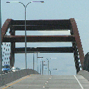
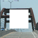
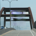
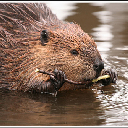
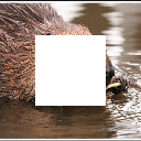
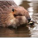
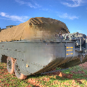
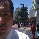
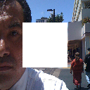
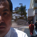
Figure 5. Comparison between CE (Pathak et al., 2016) and our PCE model, on inpainting a $64\times 64$ region in $128\times 128$ images taken from the ImageNet validation set.

Ground Truth	Input	CE	PCE

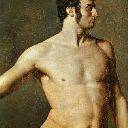
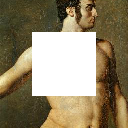
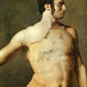
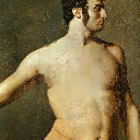
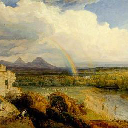
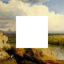
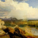
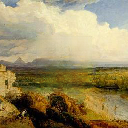
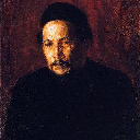
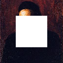
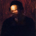
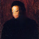
Figure 6. Comparison between CE (Pathak et al., 2016) and our PCE model, on inpainting a $64\times 64$ region in $128\times 128$ images taken from the PaintersN test set.

As our PCE model is capable of inpainting images larger than $128\times 128$, we show results on $256\times 256$ images, with a $128\times 128$ missing region in Table 4. Additionally, in this table we also show random region inpainting results. The random region inpainting models were trained without overlap between the context and the missing region.

Table 4. Center and random region inpainting results for PCE on $256\times 256$ images with a $128\times 128$ masked region. RMSE and PSNR for models trained on the ImageNet and PaintersN datasets (horizontally), and evaluated on both datasets (vertically). The first two rows are for centre region inpainting, the last two for random region inpainting.

		ImageNet		PaintersN
Region	Trained on	RMSE	PSNR	RMSE	PSNR
Center	Imagenet	$24.36$	$20.40$	$23.87$	$20.57$
	PaintersN	$24.99$	$20.17$	$23.41$	$20.74$
Random	Imagenet	$24.62$	$20.30$	$24.20$	$20.45$
	PaintersN	$25.13$	$20.13$	$24.06$	$20.51$

The results in Table 4 not only show that our model is capable of inpainting images at a higher resolution, they also show that randomising the location of the missing region only has a minimal effect on the performance of our model. Although all results were obtained by training a model specifically for the task, we note that no changes in model configuration were necessary to vary between tasks.

In Figure 7 we show several centre region inpainting examples generated by our PCE model on $256\times 256$ images.

Ground Truth	Input	PCE

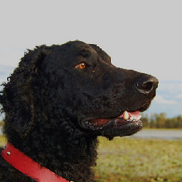
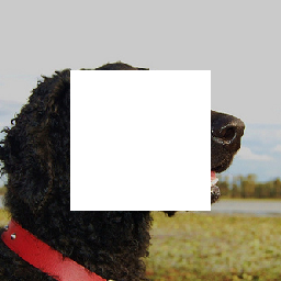
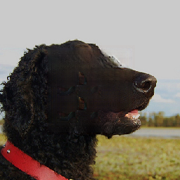
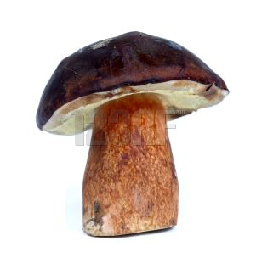
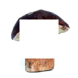
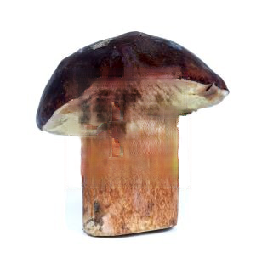
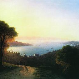
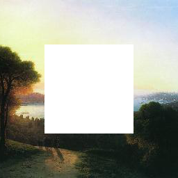
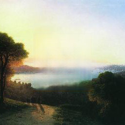
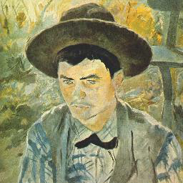
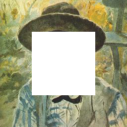
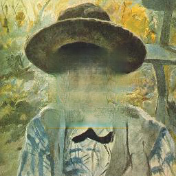
Figure 7. Examples produced by our PCE model, on inpainting a $128\times 128$ region in $256\times 256$ images taken from the ImageNet validation set in the first two rows, and PaintersN test set in the last two rows.

4.4. Image extrapolation

In this section, we explore image extrapolation; generating novel content beyond the image boundaries. By training a PCE to reconstruct the content on the boundary of an image (effectively inverting the centre region mask), we are able to teach the model to extrapolate images. In Table 5 we show the results of image extrapolation obtained by only providing the centre $192\times 192$ region of $256\times 256$ images, aiming to restore the $64$ pixel band surrounding it. For our region inpainting experiments we corrupted $\frac{1}{4}$th of the pixels, whereas for this task $\frac{9}{16}$th of the pixels are corrupted. Despite the increase in size of the reconstructed region, the difference in performance is not very large, highlighting the viability of image extrapolation with this approach.

Table 5. Image extrapolation results for PCE on $256\times 256$ images based on a provided $192\times 192$ centre region. RMSE and PSNR for models trained on the ImageNet and PaintersN datasets (horizontally), and evaluated on both datasets (vertically).

	ImageNet		PaintersN
Trained on	RMSE	PSNR	RMSE	PSNR
Imagenet	$31.81$	$18.08$	$32.82$	$17.81$
PaintersN	$32.67$	$17.85$	$32.39$	$17.92$

In Figure 8 we show four examples obtained through image extrapolation. Based on only the provided input our PCE is able to generate novel content for the $64$ pixel band surrounding the input. Although the output does not exactly match the input, the generated output does appear plausible.

Ground Truth	Input	PCE

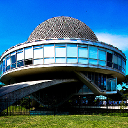
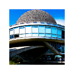
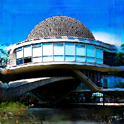
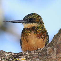
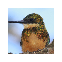
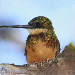
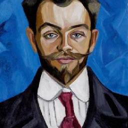
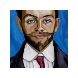
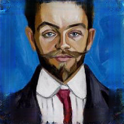
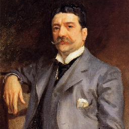
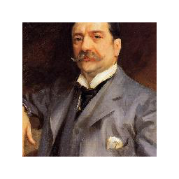
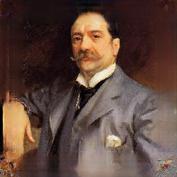
Figure 8. Examples produced by our PCE model, on extrapolating $192\times 192$ regions taken from $256\times 256$ images from the ImageNet validation set in the first two rows, and PaintersN test set in the last two rows.

Additionally, in Figure 9 we show images obtained by applying the PCE trained for image extrapolation to uncorrupted images, resized to $192\times 192$ pixels. By resizing the images to the resolution of the region the model was train on, the model will generate a band of $64$ pixels of novel content, for which there is no ground truth.

Original	PCE	Original	PCE

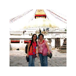
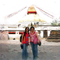
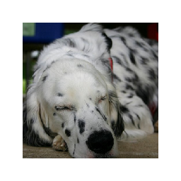
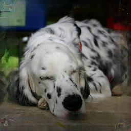
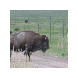
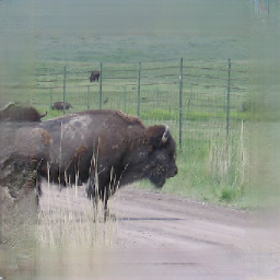
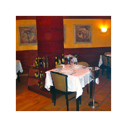
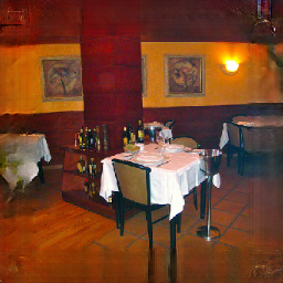
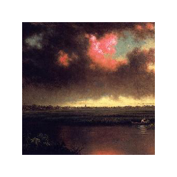
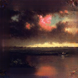
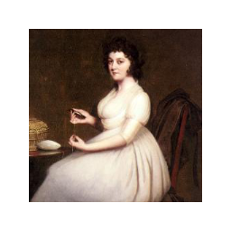
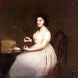
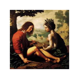
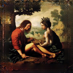
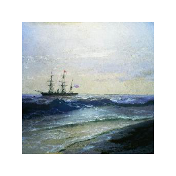
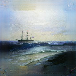
Figure 9. Examples produced by our PCE model, on extrapolating $192\times 192$ images beyond their current boundaries. The images in the first two rows are from the ImageNet validation, and in the last two rows from the PaintersN test set.

5. Conclusion

In this paper we presented a novel inpainting model: Pixel Content Encoders (PCE), by incorporating dilated convolutions and PatchGAN we were able to reduce the complexity of the model as compared to previous work. Moreover, by incorporating dilated convolutions PCE are able to preserve the spatial resolution of images, as compared to encoder-decoder style architectures which lose spatial information by compressing the input into ‘bottleneck’ representations.

We trained and evaluated the inpainting performance of PCE on two datasets of natural images and paintings, respectively. The results show that regardless of the dataset PCE were trained on they outperform previous work on either dataset, even when considering cross-dataset performance (i.e., training on natural images and evaluating on paintings, and vice versa). Based on the cross-dataset performance we pose that PCE solve the inpainting problem in a largely data-agnostic manner. By encoding the context surrounding the missing region PCE are able to generate plausible content for the missing region in a manner that is coherent with the context.

The approach presented in this paper does not explicitly take into account the artist’s style. However, we would argue that the context reflects the artist’s style, and that generated content coherent with the context is therefore also reflects the artist’s style. Future research on explicitly incorporating the artist’s style is necessary to determine whether it is beneficial for inpainting on artworks to encode the artist’s style in addition to the context.

We conclude that PCE offer a promising avenue for image inpainting and image extrapolation. With an order of magnitude fewer model parameters than previous inpainting models, PCE obtain state-of-the-art performance on benchmark datasets of natural images and paintings. Moreover, due to the flexibility of the PCE architecture it can be used for other image generation tasks, such as image extrapolation. We demonstrate the image extrapolation capabilities of our model by restoring boundary content of images, and by generating novel content beyond the existing boundaries.

References

- (1)
- Barnes et al. (2009) Connelly Barnes, Eli Shechtman, Adam Finkelstein, Dan B Goldman, and Adobe Systems. 2009. PatchMatch: A Randomized Correspondence Algorithm for Structural Image Editing. ACM Transactions on Graphics 28, 3 (2009), 24–1.
- Bertalmio et al. (2000) Marcelo Bertalmio, Guillermo Sapiro, Vicent Caselles, Coloma Ballester, Escola Superior Politecnica, and Universitat Pompeu Fabra. 2000. Image Inpainting. ACM SIGGRAPH (2000).
- Bertalmio et al. (2003) Marcelo Bertalmio, Luminita Vese, Guillermo Sapiro, and Stanley Osher. 2003. Simultaneous structure and texture image inpainting. IEEE Transactions on Image Processing 12, 8 (2003), 882–889.
- Chan et al. (2011) R H Chan, J F Yang, and X M Yuan. 2011. Alternating direction method for image inpainting in wavelet domain. SIAM J. Imaging Sci 4, 3 (2011), 807–826.
- Clevert et al. (2016) Djork-Arné Clevert, Thomas Unterthiner, and Sepp Hochreiter. 2016. Fast and Accurate Deep Network Learning by Exponential Linear Units (ELUs). arXiv preprint (2016), 1–14. arXiv:arXiv:1511.07289v5
- Cornelis et al. (2013) B. Cornelis, T. Ružić, E. Gezels, a. Dooms, a. Pižurica, L. Platiša, J. Cornelis, M. Martens, M. De Mey, and I. Daubechies. 2013. Crack detection and inpainting for virtual restoration of paintings: The case of the Ghent Altarpiece. Signal Processing 93, 3 (mar 2013), 605–619. https://doi.org/10.1016/j.sigpro.2012.07.022
- Gao and Grauman (2017) Ruohan Gao and Kristen Grauman. 2017. From One-Trick Ponies to All-Rounders: On-Demand Learning for Image Restoration. arXiv preprint (2017). arXiv:arXiv:1612.01380v2
- Giakoumis et al. (2006) Ioannis Giakoumis, Nikos Nikolaidis, and Ioannis Pitas. 2006. Digital image processing techniques for the detection and removal of cracks in digitized paintings. IEEE Transactions on Image Processing 15 (2006), 178–188.
- Glorot and Bengio (2010) Xavier Glorot and Yoshua Bengio. 2010. Understanding the difficulty of training deep feedforward neural networks. Proceedings of the 13th International Conference on Artificial Intelligence and Statistics (AISTATS) 9 (2010), 249–256. https://doi.org/10.1.1.207.2059
- Goodfellow et al. (2014) Ian J Goodfellow, Jean Pouget-abadie, Mehdi Mirza, Bing Xu, David Warde-farley, Sherjil Ozair, Aaron Courville, and Yoshua Bengio. 2014. Generative Adversarial Nets. In NIPS. 2672–2680. arXiv:arXiv:1406.2661v1
- Hays and Efros (2007) James Hays and Alexei A Efros. 2007. Scene Completion Using Millions of Photographs. ACM Transactions on Graphics 26, 3 (2007), 1–8. https://doi.org/10.1145/1239451.1239455
- Iizuka et al. (2017) Satoshi Iizuka, Edgar Simo-serra, and Hiroshi Ishikawa. 2017. Globally and Locally Consistent Image Completion. ACM Transactions on Graphics (Proc. of SIGGRAPH 2017) 36, 4 (2017), 107:1—-107:14.
- Ioffe and Szegedy (2015) Sergey Ioffe and Christian Szegedy. 2015. Batch Normalization: Accelerating Deep Network Training by Reducing Internal Covariate Shift. In ICML. JMLR, 448–456. arXiv:1502.03167 http://arxiv.org/abs/1502.03167
- Isola et al. (2016) Phillip Isola, Jun-yan Zhu, Tinghui Zhou, and Alexei A Efros. 2016. Image-to-Image Translation with Conditional Adversarial Networks. arXiv preprint (2016). arXiv:1611.07004
- Kingma and Ba (2015) Diederik P. Kingma and Jimmy Lei Ba. 2015. Adam: a Method for Stochastic Optimization. In International Conference on Learning Representations. 1–13. arXiv:arXiv:1412.6980v5
- Krizhevsky et al. (2012) Alex Krizhevsky, I Sutskever, and GE Hinton. 2012. ImageNet Classification with Deep Convolutional Neural Networks.. In Advances in Neural Information Processing Systems 25. 1097–1105. https://papers.nips.cc/paper/4824-imagenet-classification-with-deep-convolutional-neural-networks.pdf
- Pathak et al. (2016) Deepak Pathak, Jeff Donahue, Trevor Darrell, and Alexei A Efros. 2016. Context Encoders: Feature Learning by Inpainting. In CVPR. arXiv:arXiv:1604.07379v1
- Russakovsky et al. (2014) Olga Russakovsky, Jia Deng, Hao Su, Jonathan Krause, Sanjeev Satheesh, Sean Ma, Zhiheng Huang, Andrej Karpathy, Aditya Khosla, Michael Bernstein, Alexander C. Berg, and Li Fei-Fei. 2014. ImageNet Large Scale Visual Recognition Challenge. Arxiv (2014), 37. https://doi.org/10.1007/s11263-015-0816-y arXiv:1409.0575
- Sermanet and Lecun (2011) Pierre Sermanet and Yann Lecun. 2011. Traffic sign recognition with multi-scale convolutional networks. Proceedings of the International Joint Conference on Neural Networks SEPTEMBER 2011 (2011), 2809–2813. https://doi.org/10.1109/IJCNN.2011.6033589
- Solanki and Mahajan (2009) V Solanki and A R Mahajan. 2009. Digital Image Processing Approach for Inspecting and Interpolating Cracks in Digitized Pictures. International Journal of Recent Trends in Engineering (IJRTE) 1 (2009), 97–99.
- Yang et al. (2017) Chao Yang, Xin Lu, Zhe Lin, Eli Shechtman, Oliver Wang, and Hao Li. 2017. High-Resolution Image Inpainting using Multi-Scale Neural Patch Synthesis. arXiv preprint (2017). arXiv:1611.09969
- Yeh et al. (2016) Raymond Yeh, Chen Chen, Teck Yian Lim, Mark Hasegawa-johnson, and Minh N Do. 2016. Semantic Image Inpainting with Perceptual and Contextual Losses. arXiv preprint (2016). arXiv:arXiv:1607.07539v2
- Yu and Koltun (2016) Fisher Yu and Vladlen Koltun. 2016. Multi-Scale Context Aggregation by Dilated Convolutions. In Iclr. 1–9. https://doi.org/10.16373/j.cnki.ahr.150049 arXiv:1511.07122
- Yu et al. (2017) Fisher Yu, Vladlen Koltun, Intel Labs, and Thomas Funkhouser. 2017. Dilated Residual Networks. arXiv preprint (2017). arXiv:arXiv:1705.09914v1