Attractors for two dimensional waves with homogeneous Hamiltonians of degree 0

Abstract

In domains with topography, inertial and internal waves exhibit interesting features. In particular, numerical and lab experiments show that, in two dimensions, for generic forcing frequencies, these waves concentrate on attractors. The goal of this paper is to analyze mathematically this behavior, using tools from spectral theory and microlocal analysis.

1 Physical background

The mathematical problem which will be discussed in this paper is motivated by the physical observation that, in presence of topography, forcing inertial or internal waves leads to the formation of singular geometric patterns, which accumulate most of the energy.

1.1 Inertial and internal waves

Inertial and internal waves are of upmost importance in oceanic flows. They describe small departures from equilibrium in an incompressible fluid submitted respectively to the Coriolis force (due to the Earth rotation), or to the combination of density stratification and gravity. These waves are very well described when the effect of boundaries is neglected, assuming for instance that the fluid is contained in a parallelelipedic box with zero flux condition at the boundary (or equivalently in a periodic box). For the sake of completeness, we recall here the equations governing these waves, and their usual decomposition as a superposition of plane waves using the Fourier transform.

$\bullet$ Let us first consider the case of inertial waves, assuming that the density of the fluid is homogeneous $\rho(t,x)=\rho_{0}$. The incompressibility constraint states $\operatorname{div}u=0$, where $u$ is the bulk velocity of the fluid.

The (linearized) conservation of momentum provides

$$\rho_{0}({\partial}_{t}u+u\wedge\Omega)+\nabla p=0$$

denoting by $p$ the pressure, and by $\Omega$ the rotation vector. Note that there is no convection term $u\cdot\nabla u$ here as it is expected to be negligible for small fluctuations. Assuming for the sake of simplicity that $\rho_{0}=1$ and taking the divergence of this equation, we get

$$\operatorname{div}(u\wedge\Omega)+\Delta p=0$$

from which we deduce that the pressure is given by

$$p=(-\Delta)^{-1}\operatorname{div}(u\wedge\Omega)\,.$$

We therefore end up with the dynamical equation

$${\partial}_{t}u+(I+\nabla(-\Delta)^{-1}\operatorname{div})(u\wedge\Omega)=0\,.$$ (1.1)

If the rotation is constant (say in the vertical direction $\Omega=e_{3}$), we rewrite the incompressibility constraint in Fourier variables

$$p_{h}\cdot\hat{u}_{p,h}+p_{3}\hat{u}_{p,3}=0,$$

using the subscript $h$ to denote the horizontal component, and take the Fourier transform of (1.1) to get

$${\partial}_{t}\hat{u}_{p,h}+\begin{pmatrix}{p_{1}p_{2}\over|p|^{2}}&1-{p_{1}^{2}\over|p|^{2}}\\ -1+{p_{2}^{2}\over|p|^{2}}&-{p_{1}p_{2}\over|p|^{2}}\end{pmatrix}\hat{u}_{p,h}=0\,.$$

The matrix has eigenvalues $\pm i|p_{3}|/|p|$. In other words, the solution to the wave equation can be obtained as a superposition of plane waves $\exp(i(p\cdot x-\omega t))$ with dispersion relation

$$\omega=\pm{|p_{3}|\over|p|}\,.$$

$\bullet$ The model leading to internal waves is a little bit more complicated. It describes an incompressible fluid which at equilibrium is stratified in density with stable profile $\bar{\rho}(x)=\bar{\rho}(x_{3})$ with $\bar{\rho}^{\prime}(x_{3})<0$. Small perturbations will create both a velocity field $u$ and a fluctuation of the density $\rho=\bar{\rho}+\eta$.

The incompressibility constraint states as previously $\operatorname{div}u=0$. If the fluctuation around equilibrium is small, the conservation of mass

$${\partial}_{t}\rho+\operatorname{div}(\rho u)=0$$

gives at leading order

$${\partial}_{t}\eta+u\cdot\nabla\bar{\rho}=0\,.$$

The (linearized) conservation of momentum states

$$\bar{\rho}{\partial}_{t}u+\eta ge_{3}+\nabla p=0$$

denoting by $g$ the gravity constant, and by $p$ the pressure. As previously, the pressure is computed thanks to the incompressibility condition

$$-\operatorname{div}\left({1\over\bar{\rho}}\nabla p\right)=g{\partial}_{3}{\eta\over\bar{\rho}}\,.$$

In most physical systems, the variations of $\bar{\rho}$ are very small compared to its average $\rho_{0}$, and count only for the buoyancy term. The pressure is then given by

$$p=(-\Delta)^{-1}(g{\partial}_{3}\eta)\,.$$

The system of equations can be therefore reduced to get the Boussinesq approximation

$$\left\{\begin{aligned} {\partial}_{t}\eta+u_{3}\bar{\rho}^{\prime}(x_{3})=0,\\ {\partial}_{t}u_{h}+{g\over\rho_{0}}\nabla_{h}(-\Delta)^{-1}{\partial}_{3}\eta=0,\\ {\partial}_{t}u_{3}+{g\over\rho_{0}}(I+{\partial}_{33}(-\Delta)^{-1})\eta=0\,.\end{aligned}\right.$$

Assuming in addition that the stratification is affine so that $\bar{\rho}^{\prime}$ is a constant, and taking the Fourier transform of this system, we obtain that

$${\partial}_{t}\begin{pmatrix}\hat{\eta}_{p}\\ \hat{u}_{p,3}\end{pmatrix}+\begin{pmatrix}0&\bar{\rho}^{\prime}\\ {g\over\rho_{0}}\left(1-{p_{3}^{2}\over|p|^{2}}\right)&0\end{pmatrix}\begin{pmatrix}\hat{\eta}_{p}\\ \hat{u}_{3,h}\end{pmatrix}=0\,.$$

The solution can be expressed as a sum of plane waves with dispersion relation

$$\omega=\pm N{|p_{h}|\over|p|}\,,$$

where $N=(-g\bar{\rho}^{\prime}/\rho_{0})^{1/2}$ denotes the Brunt-Väisälä frequency.

Remark 1.1.

In both cases, the pressure is obtained by solving the Laplace equation. In a non periodic domain, we expect the solution to depend on the boundary conditions. The Leray projection onto divergence free vector fields defined by

$$P=(I+\nabla(-\Delta)^{-1}\operatorname{div})$$

is a non local (pseudo-differential) operator.

1.2 The effect of topography

When the domain is not periodic (or when the rotation or the Brunt-Väisälä frequency are not constant), the previous analysis fails because we cannot use the Fourier transform, and it becomes complicated to handle the Leray projection. In general, the zero-flux condition on the boundary is incompatible with any decomposition on special functions. Actually we will see that the waves exhibit a very different behaviour.

The lab experiments conducted by physicists, especially in the groups of Maas and Dauxois [16, 12, 5], consist in analyzing the response of a stratified fluid to some monochromatic forcing in different geometries. In [5] for instance, the domain is a 2D trapezium and the symmetry breaking is obtained by introducing a sloping boundary.

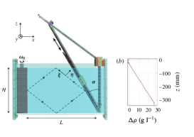
Figure 1: Experimental setup in [5].

$\bullet$ In the absence of topography (i.e. in a rectangular box which can be seen as a torus $\mathbb{T}^{2}$), the system is completely integrable and the response to the forcing can be predicted using Fourier analysis as previously.

$\bullet$ If the forcing is non resonant, i.e. if the forcing frequency $\omega_{0}$ is different from $\pm|\mathbb{p}_{h}||/|p|$ for all $p$ which are excited, then the system will oscillate according to the following equation

$${\partial}_{t}\hat{v}_{p,\pm}=\hat{f}_{p,\pm}\exp(i(\pm\omega_{p}-\omega_{0})t)$$

where $\hat{v}_{p,\pm}$ is the amplitude of the wave $\exp(i(p\cdot x\mp\omega_{p}t))$. We then obtain

$$\hat{v}_{p,\pm}=\hat{f}_{p,\pm}\left({\exp(i(\pm\omega_{p}-\omega_{0})t)-1\over i(\pm\omega_{p}-\omega_{0})}\right)\,.$$

Generically, if the forcing is regularly distributed over the domain (i.e. $f\in C^{\infty}(\mathbb{T}^{2})$), the solution will be regular: it is typically the case under the diophantine condition

$$\forall\omega_{p}\neq\omega_{0},\quad|\omega_{p}-\omega_{0}|\geq C|p|^{-\alpha}$$

which is satisfied for almost all tori.

$\bullet$ If the forcing is resonant, i.e. if the forcing frequency $\omega_{0}=\pm|p_{h}||/|p|$ for some $p$ which is excited, the fluid pumps some energy and the amplitude of the resonant mode has a linear growth in time

$$\hat{v}_{p,\pm}=\hat{f}_{p,\pm}t\,.$$

But, under the same generic condition, the solution is still regular in $x$ since the resonant mode has a nice oscillating structure $\exp(i(p\cdot x))$.

For the sake of completeness, we give in appendix the detailed computations leading to these regularity results.

$\bullet$ What is observed in the presence of topography is completely different. By PIV methods (following the displacements of small markers in the fluid), one can get a measurement of the velocity field. It happens that this velocity field is very singular with respect to the spatial variable $x$, which is unexpected from the simple model in the periodic box. The energy concentrates on some geometric patterns, which are broken lines in the 2D trapezoidal geometry with affine stratification.

Furthermore, some branches of these attractors are more energetic than others, which seems to indicate that there is a focusing mechanism due to the reflection on the slope. The geometry of these attractors, especially the number of branches, depends on the forcing frequency and on the slope.

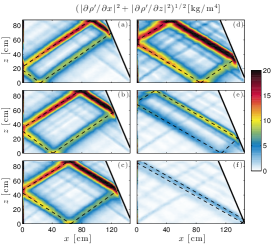
Figure 2: Experimental observation of attractors.
From the PhD thesis of C. Brouzet [5], under the supervision of T. Dauxois (ENS Lyon, 2016)

Remark 1.2.

In lab experiments, the effect of viscous dissipation is not negligible, which is important to explain that the energy varies also along each single branch. But we will not consider this effect here.

1.3 Classification of attractors

$\bullet$ The geometric pattern observed in the lab experiments coincide with the limit cycles obtained from the following geometric ray tracing

• start from any point $x_{0}$ in the domain,

• draw the ray of direction $\phi$ such that $\sin\phi=\omega_{0}/N$,

• when the ray hits the boundary, make a reflection preserving $|\sin\phi|$,

• continue this construction to obtain the limit cycle (or limit point).

This procedure is the counterpart of the geometric optics for electromagnetic or acoustic waves, the crucial difference here being that the frequency $\omega_{0}$ prescribes the direction of the propagation instead of the modulus of the wavelength.

Without entering into the details of this geometric approximation, let us just explain the intuition behind it. The idea is to look at the propagation of a wave packet, i.e. to seek for a solution in the form

$$\exp\left(i{p(t)\cdot x\over{\varepsilon}}-\frac{1}{2}(x-x(t))^{2}\right)$$

which is localized both in space (around $x(t)$) and in frequency (around $p(t)$). Unlike the plane waves obtained in the first paragraph, the time frequency in this Ansatz is not quantified, and the amplitude now depends both on $t$ and $x$.

Remark 1.3.

Of course, it is impossible to prescribe both the localization in $x$ and the localization in $p$ (which is the well-known uncertainty principle in quantum physics). The main assumption behind the geometric approximation is that there is a scale separation (measured here by the factor ${\varepsilon}$), and $p$ is the Fourier variable corresponding to $x/{\varepsilon}$.

Plugging this Ansatz in the dynamical equations, we find that the propagation of the wave packet is given at leading order by the Hamiltonian equations

$${dx_{i}\over dt}={{\partial}h\over{\partial}p_{i}},\quad{dp_{i}\over dt}=-{{\partial}h\over{\partial}x_{i}},$$

where the Hamiltonian is defined by the dispersion relation $h(x,p)=\omega(x,p)$.

For internal waves in 2D with an affine stratification (say $N=1$), we find that

$$\left\{\begin{aligned} &\frac{dx_{1}}{dt}=\frac{p_{3}^{2}}{|p|^{3}},\quad&\frac{dp_{1}}{dt}=0,\\ &\frac{dx_{3}}{dt}=-\frac{p_{3}p_{1}}{|p|^{3}},\quad&\frac{dp_{3}}{dt}=0\,.\end{aligned}\right.$$

Note that the group velocity is orthogonal to the wavenumber $p$, and that its modulus is conversely proportional to $|p|$, which are typical features from dynamics with Hamiltonian homogeneous of degree 0 (i.e. invariant by the homotheties $p\mapsto\lambda p$). This means that, on the energy level $\omega=\omega_{0}$, we have that the wavenumber $p$ satisfies

$${|p_{1}|\over|p|}=\omega_{0}$$

and the direction of propagation, which is orthogonal to $p$, makes an angle $\phi=\pm\arcsin\omega_{0}$ with respect to the horizontal.

$\bullet$ Using this ray tracing method, it is possible to construct numerically the trajectories, and investigate systematically their long time behavior.

Three scenarios appear depending on the slope $\alpha$ and on the forcing frequency $\omega_{0}=\sin\phi$, which are

• convergence to a limit cycle

• concentration in a corner,

• no emergence of a pattern

Note that, both at the experimental and numerical levels, one cannot observe very long patterns because they will be generically rather dense in the domain and the accuracy of the measurements is finite.

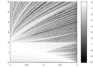
Figure 3: Greyscale: Lyapunov exponent of the trajectories.
White regions: attractors.
Black regions: no pattern emerges from the ray tracing.
From L. Maas, D. Benielli, J. Sommeria, F. Lam [16]

At the theoretical level, the long time behavior of the Hamiltonian dynamics can be characterized by exhibiting a Poincaré section, and looking at the Poincaré return map. If $\phi>\alpha$, a Poincaré section is $x_{3}=0$ and it is easy to see that all trajectories will focus on a corner. If $\phi<\alpha$, a Poincaré section is the lateral boundary $x_{1}=x_{1}^{+}(x_{3})$. The Poincaré return map $\pi_{\alpha,\phi}$ is a continuous map on the circle $\mathbb{S}^{1}$ (an homeomorphism) preserving the orientation. Such a map $\pi$ admits a crucial dynamical invariant $\rho(\pi)\in\mathbb{T}$, referred to as the rotation number, which has been introduced by Poincaré. It can be defined for instance as follows: for any $c,c^{\prime}\in\mathbb{S}^{1}\,$

$$\rho(\pi)=\lim_{n\to\infty}\frac{1}{n}|\{j\in[0,n-1]\,/\,\pi^{j}(c^{\prime})\in[c,\pi(c)[\}.$$

(we refer to the first chapter of [7] for a brief presentation of the combinatorial theory of Poincaré). Let us state the main properties of the rotation number $\rho(\pi)$.

• When the rotation number $\rho(\pi)$ is rational, $\pi$ has periodic points (having all the same period) and any orbit is asymptotic to a periodic orbit.

• When the rotation number $\rho=\rho(\pi)$ is irrational, $\pi$ is semi-conjugated to the rotation $R_{\rho}:\theta\mapsto\theta+\rho$, i.e. there exists a monotone map $h$ such that $h\circ\pi=R_{\rho}\circ h$. Note that, in general $h$ is not a bijection: the inverse image of some point may be an interval.

  In [8], Denjoy proved that, as soon as $\pi$ is smooth enough, the map $h$ is a nice continuous change of variables and $\pi=h^{-1}\circ R_{\rho}\circ h$.

For generic families of $C^{2}$ circle diffeomorphisms depending on one parameter, it has been proved by Arnold and Hermann (see Chapter 4 of [7]) that the rotation number is locally constant (as a function of this parameter), precisely when it is rational: this phenomenon is known as frequency locking. The set of parameters for which the rotation number is irrational is a Cantor set possibly with non zero Lebesgue measure (devil’s staircase). This provides bifurcation diagrams with Arnold’s tongues very similar to Fig 3. Unfortunately this theory does not apply here as the Poincaré return map is only piecewise affine. However it is clear that fixed points of the (iterated) return map are stable under small perturbations of $\alpha$ or $\phi$. We therefore preserve the band structure of the bifurcation diagram for rational rotation numbers.

2 The mathematical scenario for the formation of geometric patterns

The goal of the present paper is to provide a mathematical description of the mechanisms leading to the formation of these geometric patterns, beyond the ray approximation which is not valid here since there is no scale separation.

2.1 Quasi-resonant forcing

The first important remark is that the response to the forcing does not correspond to the usual picture when the wave operator has discrete eigenmodes. A natural question is therefore to understand the response to the forcing when the wave operator has some continuous spectrum.

A very simple example which can illustrate this mechanism is the 1D Schrödinger equation in the whole space with a monochromatic forcing (although it is not really relevant from the physical point of view):

$${\partial}_{t}\psi-i\Delta\psi=f\exp(-i\omega_{0}t)\,.$$

The interest in looking at this model is that we know explicitly the spectrum $\mathbb{R}$ and the generalized eigenfunctions $e_{\xi}:x\mapsto\exp(ix\cdot\xi)$ of the Laplacian, as well as the spectral decomposition: for any $\phi\in L^{2}(\mathbb{R})$,

$$\phi(x)={1\over 2\pi}\int_{\mathbb{R}}\hat{\phi}(\xi)\exp(ix\cdot\xi)d\xi\,$$

where the Fourier coefficients are defined by

$$\hat{\phi}(\xi)=\int_{\mathbb{R}}\phi(x)\exp(-ix\cdot\xi)dx\,.$$

In Fourier variables, the Schrödinger equation can be rewritten

$${\partial}_{t}\hat{\psi}+i|\xi|^{2}\hat{\psi}=\hat{f}\exp(-i\omega_{0}t)\,,$$

from which we deduce that

$$\hat{\psi}(t,\xi)\exp(it|\xi|^{2})=-i\hat{f}(\xi){\exp(it(|\xi|^{2}-\omega_{0}))-1\over|\xi|^{2}-\omega_{0}}\,.$$

$\bullet$ A first way of looking at this system is to consider averages: for any $\phi\in L^{2}(\mathbb{R})$, we define

$$<\psi,\phi>(t)=\int\psi(t,x)\phi^{*}(x)dx={1\over 2\pi}\int\hat{\psi}(t,\xi)\bar{\phi}^{*}(\xi)d\xi\,.$$

Using Parseval’s identity, we get

$$\exp(i\omega_{0}t)<\psi,\phi>(t)={-i\over 2\pi}\int\hat{\phi}^{*}(\xi)\hat{f}(\xi){1-\exp(-it(|\xi|^{2}-\omega_{0}))\over|\xi|^{2}-\omega_{0}}d\xi\,.$$

Recall that, if $a<\omega<b$

$$\int{1-\exp(-i(\lambda-\omega)t)\over-\omega+\lambda}{\bf 1}_{[a,b]}d\lambda =\int{1-\exp(-i\mu)\over\mu}{\bf 1}_{[(a-\omega)t,(b-\omega)t]}d\mu$$

$$=i\pi+\log{b-\omega\over\omega-a}+O(\frac{1}{t})\,,$$

We then expect that the average $<\psi,\phi>(t)$ will converge to a finite value as $t\to\infty$, at least if the forcing frequency is not 0, which corresponds to a singularity of the resonant manifold.

More precisely, we have by the simple changes of variables $|\xi|^{2}=\lambda=\omega_{0}+{1\over t}\mu$

$$2\pi<\psi,\phi> =-i\exp(-i\omega_{0}t)\int_{0}^{+\infty}{1-\exp(-i(\lambda-\omega_{0})t)\over-\omega_{0}+\lambda}\hat{f}(\sqrt{\lambda})\bar{\phi}^{*}(\sqrt{\lambda}){d\lambda\over 2\sqrt{\lambda}}$$

$$-i\exp(-i\omega_{0}t)\int_{0}^{+\infty}{1-\exp(-i(\lambda-\omega_{0})t)\over-\omega_{0}+\lambda}\hat{f}(-\sqrt{\lambda})\bar{\phi}^{*}(-\sqrt{\lambda}){d\lambda\over 2\sqrt{\lambda}}$$

$$=-i\exp(-i\omega_{0}t)\int_{-\omega_{0}t}^{+\infty}{1-\exp(-i\mu)\over\mu}F(\omega_{0}+{1\over t}\mu)d\mu\,.$$

with

$$F(z)=\frac{1}{2\sqrt{z}}(\hat{f}(\sqrt{z})\bar{\phi}^{*}(\sqrt{z})+\hat{f}(-\sqrt{z})\bar{\phi}^{*}(-\sqrt{z}))\,.$$

If we assume that both the forcing $f$ and the weight $\phi$ are smooth functions decaying at infinity,

$$\frac{2\pi}{\exp}(i\omega t)<\psi,\phi>\to-i\langle\hbox{vp}\left({1\over\lambda-\omega_{0}}\right),F\rangle+\pi F(\omega_{0})\,,$$ (2.1)

which is finite. Note that, at this stage, we do not observe any growth in time.

Remark 2.1.

Note that, in the integrable case, the amplitudes of the oscillating modes are special averages

$$\psi=\sum_{n}\hat{\psi}_{n}e_{n}\hbox{ with }\hat{\psi}_{n}=<\psi,e_{n}>$$

In the resonant case, i.e. when $\omega_{0}=\lambda_{n}$ for some $n$, the corresponding average $<\psi,e_{n}>$ grows linearly in time.

$\bullet$ Physically it can be more relevant to look at the energy, or at any observable expressed as a quadratic quantity in $\psi$. The kinetic energy for instance can be expressed in Fourier as

$$\int|\xi|^{2}|\hat{\psi}(t,\xi)|^{2}d\xi=\int\left|{1-\exp(-i(|\xi|^{2}-\omega_{0})t)\over-\omega_{0}+|\xi|^{2}}\right|^{2}\ |\hat{f}(\xi)|^{2}|\xi|^{2}d\xi\,.$$

With the same changes of variables as previously, we get

$$\int|\xi|^{2}|\hat{\psi}(t,\xi)|^{2}d\xi =\frac{1}{2}\int_{0}^{+\infty}\left|{1-\exp(-i(\lambda-\omega_{0})t)\over-\omega+\lambda}\right|^{2}(|\hat{f}(\sqrt{\lambda})|^{2}-|\hat{f}(-\sqrt{\lambda})|^{2})\sqrt{\lambda}d\lambda$$

$$=\frac{t}{2}\int_{-\omega t}^{+\infty}\left|{1-\exp(-i\mu)\over\mu}\right|^{2}G(\omega_{0}+{1\over t}\mu)d\mu$$

$$=t\int_{-\omega_{0}t}^{+\infty}{1-\cos\mu\over\mu^{2}}G(\omega_{0}+{1\over t}\mu)d\mu$$

with

$$G(z)=(|\hat{f}(\sqrt{z})|^{2}+|\hat{f}(-\sqrt{z})|^{2})\sqrt{z}\,.$$

We then conclude that generically the energy grows linearly

$$\int|\xi|^{2}|\hat{\psi}(t,\xi)|^{2}d\xi\sim{\pi\over 2}G(\omega_{0})t\,,$$ (2.2)

provided that the support of $\hat{f}$ contains $\pm\sqrt{\omega_{0}}$.

Remark 2.2.

Note that, in the integrable case, the energy is of the form

$$\sum_{n}c_{n}|\hat{\psi}_{n}|^{2}\hbox{ with }\hat{\psi}_{n}=<\psi,e_{n}>$$

In the resonant case, i.e. when $\omega_{0}=\lambda_{n}$ for some $n$, it grows quadratically in time.

The previous computations show that

• the amplitudes of linear quantities converge to some finite values (by (2.1))

• quadratic quantities grow linearly (see (2.2))

• there is essentially no energy outside bands of width $O(1/t)$ around the forcing frequency $\omega_{0}$ (which corresponds to the scaling occuring in the change of variables)

This means that the transfer of energy via quasi-resonances is quite different from the classical resonance process. The point is that the generalized eigenfunctions corresponding to the continuous part of the spectrum have infinite energy, it is therefore impossible that they emerge in finite time even though the forcing is concentrated on one frequency.

We will rephrase these properties in a more abstract setting (adapted to our study) in Section 4.

2.2 Characterization of the continuous spectrum

We therefore expect this quasi-resonant forcing to be the right mechanism to explain the formation of the geometric patterns provided that

• one can prove that the wave operator has a continuous spectrum,

• the generalized eigenfunctions exhibit some singularities on the geometric patterns.

Note that similar spectral problems had been investigated a long time ago by F. John in [15] for the 2D wave equation with Dirichlet conditions, and by J. Ralston in [23] for inertial waves in some specific 2D geometries. We will develop here a more systematic method: the key idea will be to use microlocal analysis, i.e. the connection between spectral theory and classical dynamics.

Let us first recall that a differential operator of order $m$ can be written locally

$$D=\sum_{|j|\leq m}a_{j}(x){\partial}_{x}^{j}$$

where $j$ is a multi-index of length at most $m$. Its symbol is the polynomial obtained by freezing the coefficients $a_{j}$ and taking the Fourier transform

$$d(x,p)=\sum_{|j|\leq m}a_{j}(x)(ip)^{j}\,.$$

This definition can be extended to pseudo-differential operators (involving typically inverse derivatives) by considering symbols which are more general functions than polynomials. The principal symbol $h$ of a pseudo-differential operator $H$ of order $m$ is defined in terms of the action of $H$ on fast oscillating functions $ae^{i\tau S}$, where $a$ is smooth and $S^{\prime}\neq 0$ on the support of $a$, by

$$H(ae^{i\tau S})(x)=\tau^{m}h(x,S^{\prime}(x))a(x)e^{i\tau S(x)}+O\left(\tau^{m-1}\right)$$

The function $h$ is a smooth homogeneous function of degree $m$ on $T^{\star}X\setminus 0$, which is well defined independently of the choice of local coordinates.

The key property is that the principal symbol $h\equiv h(x,p)$ of a pseudo-differential operator $H$, even though it does not determine $H$ completely, contains almost all the information, up to smoother error terms. More precisely, one defines classes of pseudo-differential operators according to the order $m$ of their symbol

$$S_{m}=\{\sigma=\sigma(x,p)\in C^{\infty}(T^{*}X\setminus X\times\{0\})\,/\,|{\partial}^{\alpha}_{x}{\partial}^{\beta}_{p}\sigma|\leq C_{\alpha,\beta}(1+|p|)^{m-|\beta|}\}\,.$$

Then, if $H$ is a pseudodifferential operator of principal symbol $h$ and order $m$, we can define another operator $Op(h)$ using the Weyl quantization

$${\rm Op}(h)u(x):=\frac{1}{(2\pi)^{{\rm dim}(X)}}\int e^{i(x-x^{\prime})\cdot p}h\left(\frac{x+x^{\prime}}{2},p\right)u(x^{\prime})\>dx^{\prime}dp$$

and compare both operators: we find that $H-{\rm Op}(h)$ is of order at most $m-1$.

Furthermore, one can prove that the symbol of the commutator $i[H_{1},H_{2}]$ is the Lie bracket $\{h_{1},h_{2}\}$, so that

$${\rm order}([H_{1},H_{2}])\leq{\rm order}(H_{1})+{\rm order}(H_{2})-1.$$

By iterating this kind of estimates, we then see that the symbolic calculus allows to obtain expansions up to any regularizing order. For a nice introduction to this subject, we refer to [1, 9, 25].

$\bullet$ Typical operators with continuous spectrum are multiplications by smooth functions $\nu=\nu(x)$ (the spectrum is then the range of $\nu$). In this case, the classical dynamics is defined by the Hamiltonian $h(x,p)=\nu(x)$

$${dx\over dt}={{\partial}h\over{\partial}p}=0,\quad{dp\over dt}=-{{\partial}h\over{\partial}x}=-\nu^{\prime}(x)=-\nu^{\prime}(x_{0})\,,$$

so that $\pm p$ is a Lyapunov function, going to infinity as $t\to\infty$.

In contrast, operators with discrete spectrum (called “elliptic operators”) have eigenfunctions of finite energy, meaning that the classical dynamics has compact invariant sets. Therefore, in this case, we cannot have any escape function as no quantity will go to infinity.

This is of course not a proof but at least a strong indication that the fact that a pseudo-differential operator $H$ has continuous spectrum is related to the existence of an escape function $d$ for the Hamiltonian dynamics associated to its principal symbol $h$

$${d\over dt}d(x(t),p(t))\geq\gamma>0$$

denoting by $(x(t),p(t))$ the trajectories of the classical dynamics:

$${dx\over dt}={{\partial}h\over{\partial}p},\quad{dp\over dt}=-{{\partial}h\over{\partial}x}\,.$$

$\bullet$ A nice mathematical tool to study the continuous spectrum of a skew-symmetric operator $iH$ (such as our wave operator) is the conjugate operator method that we will present in Section 5. The crucial point in this theory is the existence of a self-adjoint operator $D$ satisfying the commutator estimate

$$[H,D]\geq\gamma I+K\hbox{ with }\gamma>0,\hbox{ and $K$ a compact operator}\,,$$ (2.3)

Note that the existence of a conjugate operator $D$ for the wave operator $H$ can be translated in terms of the classical dynamics associated to $H$: it is roughly equivalent to the existence of an escape function $\psi$ since the condition (2.3) can be expressed in terms of the Lie bracket

$$\{h,d\}\geq\gamma>0\,.$$ (2.4)

Under this condition, the conjugate operator method shows how to extend the resolvent $(H-\lambda\pm i{\varepsilon})^{-1}$ which is defined for ${\varepsilon}>0$ and ${\varepsilon}<0$, up to ${\varepsilon}=0$

$$(H-\lambda\pm i0)^{-1}=\lim_{{\varepsilon}\to 0^{+}}(H-\lambda\pm i{\varepsilon})^{-1}\,.$$

As a consequence, on can prove that the spectral decomposition of a smooth function $f$, i.e. the measure $\nu$ defined by

$$f=\int d\nu(\lambda),\qquad\chi(H)f=\int\chi(\lambda)d\nu(\lambda)$$

is a regular function of $\lambda$ given by

$$\nu(\lambda)={1\over 2i\pi}\left((H-\lambda-i0)^{-1}f-(H-\lambda+i0)^{-1}f\right)\,.$$

The proofs of this result are not very complicated, but it is not completely obvious to get a good intuition of this property.

2.3 Classical dynamics for Hamiltonians of degree 0

The last important ingredient we will use is the fact that the existence of an escape function is a generic property of Hamiltonians of degree $0$ in dimension $2$.

Definition 2.3.

A smooth homogeneous function of degree $1$, $d:\Sigma_{\omega_{0}}\rightarrow\mathbb{R}$, is called an escape function if the Poisson bracket $\{h,d\}$, which is homogeneous of degree $0$, is strictly positive on the energy surface $\Sigma_{\omega_{0}}=h^{-1}(\omega_{0})$.

$\bullet$ Let us first have a look at the classical dynamics of internal waves in the trapezoidal geometry. The dynamical equations

$$\left\{\begin{aligned} &\frac{dx_{1}}{dt}=\frac{p_{3}^{2}}{|p|^{3}},\quad&\frac{dp_{1}}{dt}=0,\\ &\frac{dx_{3}}{dt}=-\frac{p_{3}p_{1}}{|p|^{3}},\quad&\frac{dp_{3}}{dt}=0\,.\end{aligned}\right.$$

have to be supplemented with boundary conditions. To determine the reflection laws, we look at the solutions of the Boussinesq system in some half space delimited by a slope tilted of an angle $\alpha$ with respect to the horizontal

$$x_{1}\sin\alpha+x_{3}\cos\alpha=C\,.$$

We seek these solutions in the form of an incident wave propagating with an angle $\phi$ with respect to the horizontal (recall that the direction of propagation is orthogonal to the wavenumber) plus a reflected wave

$$W=\lambda U(p)+\mu V(p)$$

$$W^{\prime}=\lambda^{\prime}U(p^{\prime})+\mu^{\prime}V(p^{\prime})$$

with

$$U(p)=\left(\begin{array}[]{c}1\\ 0\\ 0\end{array}\right)\cos(\omega t+p\cdot x)-\left(\begin{array}[]{c}0\\ -Np_{3}/(\rho^{\prime}|p|)\\ Np_{1}/(\rho^{\prime}|p|)\end{array}\right)\sin(\omega t+p\cdot x)$$

$$V(p)=\left(\begin{array}[]{c}1\\ 0\\ 0\end{array}\right)\sin(\omega t+p\cdot x)+\left(\begin{array}[]{c}0\\ -Np_{3}/(\rho^{\prime}|p|)\\ Np_{1}/(\rho^{\prime}|p|)\end{array}\right)\cos(\omega t+p\cdot x)$$

We then obtain necessary conditions on the wavenumber of the reflected wave

$$\left\{\begin{aligned} &\frac{(p^{\prime}_{1})^{2}}{|(p^{\prime})^{2}|}=\frac{p_{1}^{2}}{|p|^{2}}=\sin^{2}\phi\hbox{ coming from the conservation of energy}\\ &(p^{\prime}_{1}-p_{1})\cos\alpha-(p^{\prime}_{3}-p_{3})\sin\alpha=0\hbox{ for the phase to be constant on the slope}\end{aligned}\right.$$

as well as some polarization conditions to determine $(\lambda^{\prime},\mu^{\prime})$ from $(\lambda,\mu)$.

We will use the following reduction to represent the trajectories. Specular reflection on the horizontal and vertical boundaries is equivalent to free propagation in a domain which is extended by symmetry. Combining two successive reflections with respect to horizontal boundaries, we get a simple vertical translation, which means that we obtain a periodic structure with respect to the vertical variable. We then identify the points of the horizontal boundary in the extended domain.

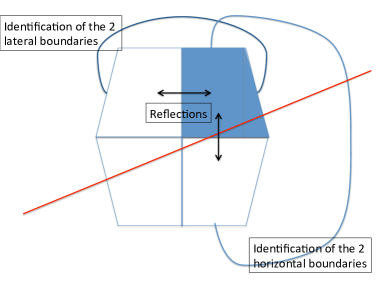
Figure 4: The image method leads to a singular dynamics in a periodic domain.

When a trajectory exits the domain on the left (resp. on the right), it re-enters on the right (resp. on the left) at the symmetric point. One can then identify the points of the lateral boundary, and get a (non smooth) dynamics on a torus, along a fixed vector field. We have actually four copies of this dynamics, corresponding to the four possible directions given by $p_{1}^{2}/|p|^{2}=\sin^{2}\phi$.

Assume that the angle $\phi$ lies in the interior of a band of the bifurcation diagram, i.e. that there exists an open set $I$ containing $\phi$ on which $\rho_{\alpha,\phi}\in\mathbb{Q}$ is constant and the periodic points are hyperbolic.

All trajectories of the semiclassical dynamics with energy $\omega_{0}=|\sin\phi|$ then converge to some attractor, corresponding to some fixed point of the (iterated) Poincaré return map $\pi_{\alpha,\phi_{0}}$. The wavenumber is exponentially increasing since it is multiplied by the same constant (depending only on $\alpha$ and $\phi$) at each iteration

$$p_{3}^{(n)}\sim C\left(\frac{\sin(\phi+\alpha)}{\sin(\alpha-\phi)}\right)^{n}\,,$$

while the distance to the limit cycle is exponentially decreasing with $n$

$$|x_{3}^{(n)}-\bar{x}_{3}|\leq C\left(\frac{\sin(\alpha-\phi)}{\sin(\phi+\alpha)}\right)^{n}\,,$$

Since the group velocity is proportional to $|p_{3}^{(n)}|^{-1}$, the return time, i.e. the time $t_{n}$ needed to run through the approximate cycle (from $x_{3}^{(n)}$ to $x_{3}^{(n+1)}$) is exponentially increasing with $n$

$$c\left(\frac{\sin(\phi+\alpha)}{\sin(\alpha-\phi)}\right)^{n}\leq|t_{n}|\leq C\left(\frac{\sin(\phi+\alpha)}{\sin(\alpha-\phi)}\right)^{n}\,.$$

In particular, the wavenumber is of the order of $O(t)$ and is therefore an escape function.

Remark 2.4.

In this example, we have exhibited an escape function, in the sense that it converges to infinity as $t\to\infty$ (with an average growth which is linear), but this function is piecewise constant with jumps. This weak notion of escape function and the lack of regularity will be major obstacles to apply the general theory.

$\bullet$ In the general case, under a suitable regularity assumption on the Hamiltonian $h$, we will actually prove that there exists a change of variables (also called normal form) such that $h-\omega_{0}$ can be locally represented by the following simple toy model on $\mathbb{T}_{x}\times\mathbb{R}_{y}$ :

$$h_{0}(x,y,\xi,\eta)={\xi\over\eta}-\lambda y\,.$$

The classical dynamics admits two first integrals $h_{0}$ and $\xi=\xi_{0}$. It is given by

$${dx\over dt}={1\over\eta},\quad{dy\over dt}=-{\xi\over\eta^{2}}\qquad{d\eta\over dt}=\lambda\,.$$

We then have, for $t\geq 0$,

$$x=x_{0}+\frac{1}{\lambda}\log\left(1+{\lambda t\over\eta_{0}}\right)\hbox{ mod}(\mathbb{Z}),\qquad y={\xi_{0}\over\lambda(\eta_{0}+\lambda t)},\qquad\eta=\eta_{0}+\lambda t\,.$$

Let us denote by $\gamma$ the curve $y=0$ in $\mathbb{T}_{x}\times\mathbb{R}_{y}$. We see that the trajectory spirals around $\gamma$ infinitely many times with a speed going to 0. Let us then look at the Poincaré map $\pi$ associated to the section $S=\{(x,y,\xi,\eta)\,/\,x=0,\xi=\lambda y\eta,\eta>0\}$ with the symplectic form given by $dy\wedge d\eta$:

$$\pi(y,\eta)=(e^{-\lambda}y,e^{\lambda}y)$$

and we have a geometric progression of momenta $\eta$, which is an escape function.

This model is therefore a smooth version of the dynamics associated to internal (or inertial) waves. We will show in Section 6 that, under rather general assumptions (stated in the next paragraph), one can always reduce the study of (smooth) Hamiltonians of degree 0 to this simple model.

3 Main results

As explained in the previous paragraph, the mathematical setting we consider in this paper reproduces the important features of the inertial and internal wave operators in domains with topography, but with more regularity in order that techniques of pseudo-differential calculus can be used.

More precisely, we consider a general scalar equation of the form

$$\frac{1}{i}{\partial}_{t}u+Hu=fe^{-i\omega_{0}t}$$ (3.1)

on a 2D torus $X$ equipped with a smooth density $dx$, where $fe^{-i\omega_{0}t}$ is a periodic smooth forcing, and $H$ is a bounded self-adjoint operator on $L^{2}(X,dx)$ satisfying the following assumptions.

(M0) $$H h:T^{*}X\setminus\{0\}\to\mathbb{R} 0$$ is a pseudo-differential operator with a smooth principal symbol positively homogeneous of degree and a vanishing subprincipal symbol.

Let us recall for the sake of completeness that the sub-principal symbol $h_{-1}$ of $H$ is the smooth homogeneous function of degree $-1$ on $T^{\star}X\setminus 0$ defined by:

$$\langle H(ae^{i\tau S})|ae^{i\tau S}\rangle_{L^{2}(X,dx)}=\int_{X}|a(x)|^{2}\left(h(x,S^{\prime}(x))+\tau^{-1}h_{-1}(x,S^{\prime}(x))\right)dx+O\left(\tau^{-2}\right)$$

Note that the function $h_{-1}$ depends on the measure $dx$.

The assumption that $h$ is homogeneous of degree 0 implies that any energy shell $\Sigma_{\omega}=h^{-1}(\omega)$ is conic:

$$\forall(x,p)\in\Sigma_{\omega},\forall\lambda\in\mathbb{R}^{+},\quad(x,\lambda p)\in\Sigma_{\omega}\,.$$

We will then denote by $Z$ the oriented manifold of dimension $2$ which is the quotient of the conic energy shell $\Sigma_{\omega_{0}}$ by the positive homotheties

$$Z=\{(x,e)\in X\times S^{1}\,/\,h(x,e)=\omega_{0}\}\,.$$

We can think of $Z$ as the boundary at infinity of the energy shell.

For the sake of simplicity, we now introduce some geometrical assumptions on $\Sigma_{\omega_{0}}$ (and $Z$) in order to avoid singularities. These assumptions can actually be relaxed as shown by the first author in the recent paper [6].

(M1) The energy shell $$\Sigma_{\omega_{0}} \pi:Z\rightarrow X n$$ is nondegenerate and the canonical projection is a finite covering of degree .

The non degeneracy assumption means that $dh\neq 0$ on $\Sigma_{\omega_{0}}$, it is a generic assumption on the frequency $\omega_{0}$ thanks to Sard’s theorem. The second assumption means that, for each $x\in X$, the pre-image of $x$ by the canonical projection $\pi$ has exactly $n$ elements, and the directions in $\pi^{-1}(x)$ are smoothly dependent on $x$. Note that, in the case of internal waves in a trapezium, the number of admissible directions $n$ at each regular point $x$ is 4, but there are singularities.

By definition, the Hamiltonian vector field $X_{h}$ is tangent to $\Sigma_{\omega_{0}}$ and homogeneous of degree $-1$. This implies that the oriented direction of $X_{h}$ induces a field of oriented directions on $Z$. We therefore say that $Z$ is equipped with a 1D-foliation, denoted by ${\cal F}$. The leaves of this foliation correspond to the orbits of the Hamiltonian dynamics in $Z$ (which are defined modulo a positive change of time). The compact leaves correspond to periodic orbits.

Note that the foliation is on $Z$. The projection on $X$ is a multiple foliation, meaning that at each point of $X$ there are $n$ distinct oriented directions.

Lemma 3.1.

Under the assumption (M1), the foliation ${\cal F}$ is non singular.

Proof.

Assume that the foliation ${\cal F}$ is singular.

Since $\Sigma_{\omega_{0}}$ is nondegenerate, the foliation can be singular only at the points where $X_{h}$ is parallel to the cone direction. The projection of the foliation ${\cal F}$ on $X$ is generated by the vectors $(\partial_{p_{1}}h,\partial_{p_{2}}h)$. Therefore the foliation ${\cal F}$ is singular if and only if this vector vanishes.

But then the tangent space to $\Sigma_{\omega_{0}}$, which is defined by the non trivial equation $(\partial_{x_{1}}h)\,dx_{1}+(\partial_{x_{2}}h)\,dx_{2}=0$, does not project in a surjective way on the tangent space of $X$. This contradicts our assumption that the canonical projection is a finite covering of degree $n$.

Note that we also retrieve the property that the wave number $p$ is orthogonal (for the duality) to the direction of the projection of $X_{h}$ on $X$. This is due to the Euler relation $p_{1}\partial_{p_{1}}h+p_{2}\partial_{p_{2}}h=0$. Another way to interpret this last condition is to say that the cones generated by the leaves of ${\cal F}$ are Lagrangian. ∎

The last assumption is on the dynamics of ${\cal F}$:

$$\hbox{\bf(M2) The foliation ${\cal F}$ is Morse-Smale},$$

which is a generic condition. Let us recall what it means:

• there is a finite number of compact leaves (diffeomorphic to circles), also called cycles in the sequel.

• Each compact leaf is hyperbolic (the corresponding linear Poincaré map - which is defined intrinsically - is strictly expanding or contracting).

• And all other leaves are accumulating only along two of the previous closed leaves at $\pm\infty$.

Note that conditions $(M1)$ and $(M2)$ are stable under small perturbations, therefore are still verified for energy levels close to $\omega_{0}$.

Remark 3.2.

The regularity assumption is encoded in $(M0)$. In particular, at this stage, even though we can capture the effect of the zero flux condition for internal waves in a model without boundary (see Fig. 4), this model is not smooth enough to enter in this class of operators.

- If the boundary is a polygon, we have seen that the Poincaré map is only piecewise affine. This difficulty could be removed by considering a smooth domain, which leads to a foliation with singular points (corresponding to critical angles). But our results can actually be extended to singular foliations (see [6]).

- A more serious difficulty comes from the fact that the wavenumber $p$ jumps at each return time, which means that there is no smooth normal form which conjugates the geometric object given by the foliation and the Hamiltonian dynamics.

To tackle the original problem, we would probably need to introduce another covering to take into account this additional complexity.

In this abstract setting, we can now formulate our result describing the long time behavior of the forced system.

Theorem 3.1.

Let $H$ be a pseudo-differential operator such that assumptions $(M0)(M1)(M2)$ are satisfied for any $\omega_{0}$ in some (open) interval $I$.

Then $H$ has at most a finite number of eigenvalues in $I$, and for any $\omega_{0}\in I\setminus\sigma_{pp}(H)$ and any $f\in C^{\infty}(X)$, the solution to the forced equation

$$-i{\partial}_{t}u+Hu=fe^{-i\omega_{0}t},\qquad u_{|t=0}=0$$

can be decomposed in a unique way as

$$u(t)e^{i\omega_{0}t}=u_{\infty}+b(t)+\epsilon(t)$$

where

• $u_{\infty}=(H-\omega_{0}-i0)^{-1}f$ belongs to the Sobolev spaces $\mathcal{H}^{-1/2-0}$ and is not in $L^{2}$ except if it vanishes;

• $b(t)$ is a bounded function with values in $L^{2}$ whose time Fourier transform vanishes near $0$;

• $\epsilon(t)$ tends to $0$ in $\mathcal{H}^{-1/2-0}$.

The wavefront set of the limiting distribution $WF(u_{\infty})$ is contained in the cones generated by the stable cycles of ${\cal F}$.

Furthermore, the energy $\|u(t)\|^{2}_{L^{2}(X,dx)}$ grows linearly except if $u_{\infty}$ vanishes.

Roughly speaking, the wave front set $WF(u_{\infty})$ characterizes the singularities of the generalized function $u_{\infty}$, not only in space, but also with respect to its Fourier transform at each point. In more familiar terms, $WF(u_{\infty})$ tells not only where the function $u_{\infty}$ is singular, but also how or why it is singular, by being more exact about the direction in which the singularity occurs.

More precisely, if $u$ is a Schwartz distribution on $\mathbb{R}^{d}$, $(\bar{x},\bar{p})\notin WF(u)$ means that there exists a test function $a$ with $a(\bar{x})\neq 0$ so that the Fourier transform of $au$ is fast decaying in $p$ in some conic neighborhood of $\bar{p}$, or in other words that there exists a pseudo-differential operator $A$ elliptic at the point $(\bar{x},\bar{p})$ so that $Au$ is smooth. This definition is completely intrinsic, and can be extended for a smooth manifold $X$. We refer to [25, 4] for a simple introduction to the wavefront set.

We will give in Theorem 7.1 a much more precise description of $u_{\infty}$ as a Lagrangian state (or Fourier integral distribution) associated to the previous conic Lagrangian manifolds.

Note that Dyatlov and Zworski have obtained recently [10] an alternative proof of a slightly weaker result, based only on microlocal techniques and radial estimates.

4 Quasi-resonances and long time behaviour

We first show how the (local) spectral representation of $H$ can be used to describe the long time behaviour of the solution to the forced equation. The solution $u$ of (3.1) is given by

$$u(t)=\frac{e^{-it\omega_{0}}-e^{-it{H}}}{H-\omega_{0}}f$$

Assume that $H$ has some continuous spectrum around $\omega_{0}$, and that we know the spectral decomposition of $f$ with respect to $H-\omega_{0}$:

$$\chi(H-\omega_{0})f=\int_{\mathbb{R}}\chi(s)d\nu(s)\,.$$

We thus have that

$$u(t)=e^{-it\omega_{0}}\int\frac{1-e^{-its}}{s}d\nu(s)\,.$$

We will then use a general result on oscillating integrals, extending the computations of Section 2.1:

Lemma 4.1.

Let $\mathcal{B},\mathcal{B}_{0}\subset\mathcal{B}$ be two Banach spaces. Let $\nu=\nu_{\rm ac}+\nu_{\rm sing}$ be a compactly supported Radon measure on $\mathbb{R}$ with values in $\mathcal{B}$ such that

• the absolutely continuous part $\nu_{\rm ac}$ has a density $m$ which is Hölder continuous $C^{0,\mu}$ ($\mu>0$) near $0$;

• the singular part $\nu_{\rm sing}$ has values in $\mathcal{B}_{0}$ and is supported outside from 0.

Then the oscillating integral $I(t)=\langle(1-e^{-its})s^{-1}|d\nu(s)\rangle$ can be decomposed in a unique way as

$$I(t)=I_{\infty}+b(t)+\epsilon(t)$$

where $I_{\infty}=\langle(s-i0)^{-1}|d\nu(s)\rangle\in\mathcal{B}$, $\epsilon(t)\rightarrow 0$ in $\mathcal{B}$ as $t\rightarrow\infty$, and $b$ is bounded with values in $\mathcal{B}_{0}$ and inverse Fourier transform supported on $\operatorname{supp}(\nu_{\rm sing})$.

Proof.

The proof is actually a simple calculation on distributions. Let $a>0$ be such that

$$[-a,a]\cap\operatorname{supp}(\nu_{sing})=\emptyset\,.$$

Since $\nu$ is compactly supported, there is no issue of convergence at infinity. We then split the integral into two parts:

$$I_{1}(t)=\int_{|s|<a}\frac{1-e^{-its}}{s}d\nu_{ac}+\int_{|s|\geq a}\frac{1}{s}d\nu_{ac}$$

$$I_{2}(t)=-\int_{|s|\geq a}\frac{e^{-its}}{s}d\nu_{ac}+\int_{|s|\geq a}\frac{1-e^{-its}}{s}d\nu_{sing}\,.$$

We check that the second term in $I_{2}(t)$ satisfies the properties required for $b(t)$, while the first term in $I_{2}(t)$ tends to $0$ thanks to the Riemann-Lebesgue theorem.

We have then to study $I_{1}(t)$. As $m$ is of class $C^{0,\mu}$ near 0, we have that $m_{1}(s)=(m(s)-m(0))/s$ belongs to $L^{1}$, so that

$$I_{1}(t)= \int_{|s|<a}\frac{1-\cos(ts)}{s}(m(0)+sm_{1}(s))ds$$

$$+i\int_{|s|<a}\frac{\sin(ts)}{s}(m(0)+sm_{1}(s))ds+\int_{|s|\geq a}\frac{1}{s}d\nu_{ac}$$

The second integral converges to $i\pi m(0)$. Using the parity of $\cos$ and the Riemann-Lebesgue theorem, we obtain that the first integral tends to

$$\int_{|s|<a}\frac{m(s)-m(0)}{s}ds={\rm p.v.}\left(\int_{|s|<a}\frac{m(s)}{s}ds\right)\,.$$

Adding the third term, we can remove the truncation.

In the limit, we get finally

$${\rm p.v.}\left(\int\frac{m(s)}{s}ds\right)+i\pi m(0)=\langle(s-i0)^{-1}|m\rangle$$

by the Sokhotski-Plemelj theorem. ∎

5 The conjugate operator method

In order to describe the response of the system to some monochromatic forcing at frequency $\omega_{0}$, we therefore need to get the spectral structure of $H$ close to this frequency, assuming that it is non degenerate in the sense of assumptions (M1)(M2). We will first show how to define the spectral density, assuming the existence of a conjugate operator.

5.1 A short review on Mourre theory

Let $H$ be a self-adjoint operator on some Hilbert space, say $L^{2}$. Here we will further assume that $H$ is bounded, as it is the case in the application we have in mind.

Definition 5.1.

Let $D$ be a self-adjoint (unbounded) operator. For any operator $A$, we denote by $i[A,D]$ the closure of the form $i(AD-DA)$ defined on $\mathcal{D}(A)\cap\mathcal{D}(D)$.

• We say that $H$ is $n-$smooth with respect to $D$ if the iterated brackets ${B}_{1}:=i[{H},D]$ and ${B}_{k}:=[{B}_{k-1},D]$ are bounded up to $k=n$.

• We define also the Sobolev scale $\mathcal{H}^{s}$ ($s\in\mathbb{R}$) associated to $D$ by

  $$\mathcal{H}^{s}=\{u\in L^{2}\,/\,(1+D^{2})^{s/2}u\in L^{2}\}$$

  for $s\geq 0$, and as the dual of $\mathcal{H}^{-s}$ for $s<0$.

The main result of the conjugate operator theory (see [18, 14]) is the following theorem:

Theorem 5.1 (Mourre).

Let us assume that $H$ is $n-$smooth with respect to $D$ with $n\geq 2$, and that we have the following commutator estimate: for $\chi,\bar{\chi}\in C_{0}^{\infty}(\mathbb{R},\mathbb{R}^{+})$ with $\chi\bar{\chi}=\bar{\chi}$,

$$\chi(H){B}_{1}\chi(H)\geq\alpha\bar{\chi}(H)+K\quad\hbox{ for some compact operator $K$}.$$ (5.1)

Then, for any closed interval $I\subset\operatorname{supp}(\bar{\chi})$

• $H$ has a finite set $\sigma_{p}(H)$ of eigenvalues of finite multiplicity in $I$;

• the resolvent $({H}-z)^{-1}$ defined for $\Im(z)\neq 0$ admits boundary values at the points $\omega\in I\setminus\sigma_{p}(H)$ in the space $O_{s}:=L(\mathcal{H}^{s},\mathcal{H}^{-s})$ for $s>1/2$.

• the boundary values $({H}-\omega\pm i0)^{-1}$ are Hölder continuous $C^{0,\mu}(I\setminus\sigma_{p}(H),O_{s})$ with $s>1/2$ and $\mu=(2s-1)/2s$.

• the boundary values $({H}-\omega\pm i0)^{-1}$ admits continuous derivatives of order $n$ in the spaces $O_{s}$ with $s>n-1/2$.

Proof.

For the sake of completeness, we give here a sketch of proof of a slightly simpler result, which turns out to be quite simple in our case since $H$ and $B_{1}$ are bounded operators in $L^{2}$.

$\bullet$ The first step is to prove that the discrete spectrum in the interval $I$ is finite. If it is not, there exists a sequence of orthonormal eigenfunctions $\phi_{n}$ with $H\phi_{n}=\omega_{n}\phi_{n}$. By the commutator estimate (5.1), we then get

$$0=\langle\phi_{n},B_{1}\phi_{n}\rangle\geq\alpha\|\phi_{n}\|^{2}+\langle\phi_{n},K\phi_{n}\rangle\,.$$

Since the $\phi_{n}$ are orthogonal, $\phi_{n}\rightharpoonup 0$ weakly in $L^{2}$, and since $K$ is compact,

$$\lim_{n\to\infty}\langle\phi_{n},K\phi_{n}\rangle=0\,.$$

We obtain a contradiction.

$\bullet$ The second step is to define some suitable approximation for the resolvent, when $\omega_{0}$ is not an eigenvalue of $H$. Define $P_{\delta}$ to be the spectral projector of $H$ on $[\omega_{0}-\delta,\omega_{0}+\delta]$. As $\delta\to 0$, $P_{\delta}$ converges weakly to 0, and since $K$ is compact, $KP_{\delta}\to 0$. One can then find $\delta$ small enough so that $\pm 2P_{\delta}KP_{\delta}\leq\alpha P_{\delta}^{2}$, from which we deduce that

$$P_{\delta}B_{1}P_{\delta}\geq\frac{\alpha}{2}P_{\delta}^{2}\,.$$ (5.2)

In the sequel we will remove the subscript $\delta$ and call $P$ this spectral projection.

We then define $BB^{*}=P_{\delta}B_{1}P_{\delta}$ and

$$G_{z}({\varepsilon})=(H-z-i{\varepsilon}BB^{*})^{-1},\quad F_{z}({\varepsilon})=A_{\varepsilon}G_{z}({\varepsilon})A_{\varepsilon}\,,$$

where $A_{\varepsilon}=|D+i|^{-s}|{\varepsilon}D+i|^{s-1}$ for some $s>1/2$ and ${\varepsilon}>0$. When ${\varepsilon}$ and $\Im z$ have the same sign, as $H$ is self-adjoint,

$$\|(H-z-i{\varepsilon}BB^{*})\varphi\|^{2} =\|(H-\Re z)\varphi\|^{2}+\|(\Im z+{\varepsilon}BB^{*})\varphi\|^{2}-2\Im((H-\Re z)\varphi,{\varepsilon}BB^{*}\varphi)$$

$$\geq(\Im z)^{2}\|\varphi\|^{2}$$

so that $H-z-i{\varepsilon}BB^{*}$ is injective with closed range in $L^{2}$. Since its adjoint is also injective, the range is actually $L^{2}$. By the open mapping theorem, its inverse $G_{z}({\varepsilon})$ exists as a bounded operator.

Using (5.2) and the fact that $\Im z\geq 0$, we also have that

$$\|PG_{z}({\varepsilon})A_{\varepsilon}\|^{2} =\|A_{\varepsilon}\bar{G}_{z}({\varepsilon})P^{2}G_{z}({\varepsilon})A_{\varepsilon}\|$$

$$\leq\frac{2}{\alpha{\varepsilon}}\|A_{\varepsilon}\bar{G}_{z}({\varepsilon})({\varepsilon}BB^{*}+\Im z)G_{z}({\varepsilon})A_{\varepsilon}\|$$

$$\leq\frac{1}{\alpha{\varepsilon}}\|A_{\varepsilon}(\bar{G}_{z}({\varepsilon})-G_{z}({\varepsilon}))A_{\varepsilon}\|$$

$$\leq\frac{2}{\alpha{\varepsilon}}\|A_{\varepsilon}G_{z}({\varepsilon})A_{\varepsilon}\|\leq\frac{2}{\alpha{\varepsilon}}\|F_{z}({\varepsilon})\|$$

Finally, using the spectral localization, we have that for any $z$ such that $\Re z\in[\omega_{0}-\delta/2,\omega_{0}+\delta/2]$

$$\|(I-P)G_{z}({\varepsilon})A_{\varepsilon}\|\leq C_{\delta}.$$ (5.3)

In particular, one has

$$\|G_{z}({\varepsilon})A_{\varepsilon}\|\leq C_{\alpha,\delta}\left(1+\left(\frac{\|F_{z}({\varepsilon})\|}{{\varepsilon}}\right)^{\frac{1}{2}}\right)\,.$$ (5.4)

Note that, at this stage, we did not use the specific form of $A_{\varepsilon}$. In particular, we have that

$$\|G_{z}({\varepsilon})\|\leq\frac{C}{{\varepsilon}}\,.$$ (5.5)

$\bullet$ The third step is to obtain a differential inequality in order to control the dependence with respect to ${\varepsilon}$. Let us compute the derivative of $F_{z}({\varepsilon})$ with respect to ${\varepsilon}$:

$$\frac{dF_{z}({\varepsilon})}{d{\varepsilon}} ={dA_{\varepsilon}\over d{\varepsilon}}G_{z}({\varepsilon})A_{\varepsilon}+A_{\varepsilon}G_{z}({\varepsilon}){dA_{\varepsilon}\over d{\varepsilon}}$$

$$\quad+A_{\varepsilon}G_{z}({\varepsilon})P[D,H]PG_{z}({\varepsilon})A_{\varepsilon}\,.$$

A straightforward computation shows that

$$P[D,H]P=[D,H-z-i{\varepsilon}BB^{*}]+[D,i{\varepsilon}BB^{*}]+(P-I)[D,H]P+[D,H](P-I)$$

from which we deduce that

$$\frac{dF_{z}({\varepsilon})}{d{\varepsilon}} ={dA_{\varepsilon}\over d{\varepsilon}}G_{z}({\varepsilon})A_{\varepsilon}+A_{\varepsilon}G_{z}({\varepsilon}){dA_{\varepsilon}\over d{\varepsilon}}+A_{\varepsilon}\left(-DG_{z}({\varepsilon})+G_{z}({\varepsilon})D\right)A_{\varepsilon}$$

$$\quad+{\varepsilon}A_{\varepsilon}G_{z}({\varepsilon})[D,iB^{*}B]G_{z}({\varepsilon})A_{\varepsilon}$$

$$\quad+A_{\varepsilon}G_{z}({\varepsilon})(P-I)[D,H]PG_{z}({\varepsilon})A_{\varepsilon}+A_{\varepsilon}G_{z}({\varepsilon})[D,H](P-I)G_{z}({\varepsilon})A_{\varepsilon}$$

Since the commutators $[D,BB^{*}]$ and $[D,H]$ are bounded, and that

$$\left\|{dA_{\varepsilon}\over d{\varepsilon}}\right\|=(1-s)\left\||D+i|^{-s}|D||{\varepsilon}D+i|^{s-2}\right\|\leq(1-s){\varepsilon}^{s-1}\,,$$ (5.6)

$$\|A_{\varepsilon}D\|=\left\||D+i|^{-s}|D||{\varepsilon}D+i|^{s-1}\right\|\leq{\varepsilon}^{s-1}\,.$$

we deduce from the a priori estimates (5.3)(5.4) that

$$\left\|\frac{dF_{z}({\varepsilon})}{d{\varepsilon}}\right\|\leq C{\varepsilon}^{s-1}\left(1+\left(\frac{\|F_{z}({\varepsilon})\|}{{\varepsilon}}\right)^{\frac{1}{2}}+\|F_{z}({\varepsilon})\|\right)\,.$$ (5.7)

$\bullet$ The fourth step is then to extend the resolvent as ${\varepsilon}\to 0$ by a continuity argument. By (5.7) and (5.4), we get that

$$\left\|\frac{dF_{z}({\varepsilon})}{d{\varepsilon}}\right\|\leq C{\varepsilon}^{s-3/2}\left({\varepsilon}+\|F_{z}({\varepsilon})\|\right)^{1/2}\,,$$

which upon integration shows that $\|F_{z}({\varepsilon})\|$ is uniformly bounded with respect to ${\varepsilon}$, and that $\|F_{z}({\varepsilon})-F_{z}({\varepsilon}^{\prime})\|$ goes to 0 as ${\varepsilon},{\varepsilon}^{\prime}\to 0$.

This proves in particular that $({H}-z)^{-1}$ defined for $\Im(z)>0$ admits boundary values at the points $\omega\in[\omega_{0}-\delta/2,\omega_{0}+\delta/2]$ in the space $O_{s}:=L(\mathcal{H}^{s},\mathcal{H}^{-s})$. Furthermore,

$$\left\|F_{z}({\varepsilon})-F_{z}(0)\right\|\leq C{\varepsilon}^{2s-1}\,.$$ (5.8)

$\bullet$ To obtain the Hölder continuity with respect to $z$, we compute

$$\frac{dF_{z}({\varepsilon})}{dz}=A_{\varepsilon}G_{z}({\varepsilon})G_{z}({\varepsilon})A_{\varepsilon}\,.$$

Using the uniform bound on $F_{\varepsilon}(z)$ and (5.4), we obtain that

$$\left\|\frac{dF_{z}({\varepsilon})}{dz}\right\|\leq\frac{C}{{\varepsilon}}\,.$$

Then,

$$\|F_{z}({\varepsilon})-F_{z^{\prime}}({\varepsilon})\|\leq\frac{C}{{\varepsilon}}|z-z^{\prime}|\,.$$

Combining this estimate with (5.8) and choosing ${\varepsilon}^{2s}=|z-z^{\prime}|$, we get

$$\|F_{z}(0)-F_{z^{\prime}}(0)\|\leq C|z-z^{\prime}|^{\mu}\quad\hbox{ for }\mu=(2s-1)/(2s)\,.$$

The additional regularity is obtained by defining a refined approximation of the resolvent

$$\bar{G}_{\varepsilon}(z) =(H-z-i\sum_{j=1}^{n}{{\varepsilon}^{j}\over j!}B_{j})^{-1},$$

$$\bar{F}_{\varepsilon}(z) =|D+i|^{-s}|{\varepsilon}D+i|^{s-n}G_{\varepsilon}(z)|D+i|^{-s}|{\varepsilon}D+i|^{s-n}\hbox{ with }s>n-1/2\,,$$

and by looking at higher order derivatives of $\bar{F}_{z}({\varepsilon})$. We refer to [14] for the details of this proof.

∎

5.2 Scattering for the evolution problem

A refinement of the conjugate operator method allows actually to prove that there exists a direction of propagation for the evolution $\exp(-itH)$. We indeed have the following theorem

Theorem 5.2 (Mourre).

Let us assume that $H$ is at least $2-$smooth with respect to $D$, and that the commutator estimate (5.1) holds. Denote by $P_{D}^{-}$ the spectral projectors of $D$ on $\mathbb{R}^{-}$. Then,

$$\sup_{\lambda\in I}\|P_{D}^{-}(H-\lambda-i0)^{-1}|D+i|^{-s}\|\leq C\hbox{ for }s>1\,.$$

Sketch of proof.

The arguments here are quite similar to those used in the proof of Theorem 5.1. We define for $\Im(z)>0$, $\epsilon>0$ and $s>1$

$$G_{z}({\varepsilon})=(H-z-i{\varepsilon}BB^{*})^{-1},\quad\tilde{F}_{z}({\varepsilon})=P_{D}^{-}e^{{\varepsilon}D}G_{z}({\varepsilon})|D+i|^{-s}\,.$$

$\bullet$ Let us now look at the derivative of $\tilde{F}_{z}({\varepsilon})$ with respect to ${\varepsilon}$.

$$\frac{d\tilde{F}_{z}({\varepsilon})}{d{\varepsilon}}=P_{D}^{-}e^{{\varepsilon}D}\left(DG_{z}({\varepsilon})-G_{z}({\varepsilon})P[H,D]PG_{z}({\varepsilon})\right)|D+i|^{-s}\,.$$

The same decomposition as previously shows that

$$\frac{d\tilde{F}_{z}({\varepsilon})}{d{\varepsilon}} =P_{D}^{-}e^{{\varepsilon}D}G_{z}({\varepsilon})D|D+i|^{-s}$$ (5.9)

$$\quad+{\varepsilon}P_{D}^{-}e^{{\varepsilon}D}G_{z}({\varepsilon})[D,iB^{*}B]G_{z}({\varepsilon})|D+i|^{-s}$$

$$\quad+P_{D}^{-}e^{{\varepsilon}D}G_{z}({\varepsilon})(P-I)[D,H]G_{z}({\varepsilon})|D+i|^{-s}$$

$$\quad+P_{D}^{-}e^{{\varepsilon}D}G_{z}({\varepsilon})P[D,H](P-I)G_{z}({\varepsilon})|D+i|^{-s}$$

Note that the exponential term introduces a shift, so that the derivative $D$ acts only on the right in the first term. From (5.3)(5.4)(5.5) and the bound on $\|F_{\varepsilon}(z)\|$, we have by interpolation that for any $\eta>0$, there exist $C_{\eta}>0$ and $\eta^{\prime}>0$ such that

$$\|G_{z}({\varepsilon})|D+i|^{-\eta}\|\leq C_{\eta}{\varepsilon}^{\eta^{\prime}-1}\,.$$

In particular, the three first terms in the right hand side of (5.9) are integrable.

$\bullet$ The difficulty here is to get a control on the last term, and more precisely to prove that $[D,H](P-I)G_{z}({\varepsilon})|D+i|^{-s}$ is a bounded operator from $L^{2}$ to $\mathcal{H}^{\eta}$ for some $\eta>0$.

We start from the following identity

$$(P-I)G_{z}({\varepsilon})|D+i|^{-s} =(P-I)G_{z}(0)\big{(}1+i{\varepsilon}B^{*}BG_{z}({\varepsilon})\big{)}|D+i|^{-s}$$

$$=(P-I)G_{z}(0)|D+i|^{-s}+o({\varepsilon}^{1/2})$$

where the remainder is estimated by (5.4).

We then have to prove that $|D|^{\eta}[D,H](P-I)G_{z}(0)|D+i|^{-s}$ is a bounded operator. The idea is to use the fact that, for any bounded operator $C$ and for any $\eta\in[0,1[$

$$\hbox{ if $[C,D]$ is bounded, then }|D|^{\eta}C|D+i|^{-1}\hbox{ is bounded.}$$

The proof of this statement can be found in [19]. In our case, $C=[D,H](P-I)G_{z}(0)$ is indeed a bounded operator, and the commutator can be expressed in terms of $[D,H]$ and $[D,[D,H]]$ which are bounded as well.

The last term in the right hand side of (5.9) is also integrable. We then obtain that $\|\tilde{F}_{z}({\varepsilon})\|$ has no singularity as ${\varepsilon}\to 0$.

∎

6 Spectral decomposition of the wave operator

6.1 Construction of a global escape function

As explained in the introduction, the existence of a conjugate operator for a pseudo-differential operator $H$ of principal symbol $h$ is related to the fact that the Hamiltonian dynamics of $h$ admits an escape function. The construction of the escape function $d$ is therefore the heart of the proof.

Proposition 6.1.

Under the assumptions (M0), (M1) and (M2), there exists an escape function $d$ for the Hamiltonian $h$ on $\Sigma_{\omega_{0}}$.

The function $d$ can then be extended to energies close to $\omega_{0}$.

We start by constructing a local change of variables, also called normal form, on each basin of attraction (resp. of repulsion) of the dynamics, in order to have a simple expression for the Hamiltonian $h$.

Lemma 6.2.

Let $\gamma$ be a hyperbolic closed leaf of the foliation ${\cal F}$ with Lyapunov exponent $e^{-2\pi\lambda}\neq 1.$ Denote by $B_{\gamma}$ the basin of attraction (or “repulsion”) of $\gamma$. There exists a diffeomorphism of $B_{\gamma}$ on $(\mathbb{R}/2\pi\mathbb{Z})_{x}\times\mathbb{R}_{y}$ so that the foliation is given by $dy+\lambda ydx=0$ oriented by $dx>0$.

Proof.

Up to a change of orientation, we can assume that $\gamma$ is a stable cycle.

$\bullet$ The first step is to construct the normal form close to the cycle. Let $S$ be a local Poincaré section transverse to $\gamma$. By definition, the Poincaré return map $\pi$ sends $S$ on itself. By Sternberg’s linearization theorem for 1D maps [26], there is a chart $(I,0)\subset(\mathbb{R}_{y},0)$ of $S$ so that

$$P(y)=\mu y\hbox{ with }0<\mu=e^{-2\pi\lambda}<1.$$

We then choose the normalisation of the vector field $V$ tangent to the foliation ${\cal F}$ so that the return time is $2\pi$. And we denote by $x$ the coordinate starting from $0$ along $S$ and so that $V.{x}=1$. By construction, $x\in\mathbb{R}/2\pi\mathbb{Z}$. This construction provides a foliation ${\cal F}_{0}$ given by $dy+\lambda ydx=0$ and oriented by $dx>0$.

We have now two periodic foliations ${\cal F}$ and ${\cal F}_{0}$: they agree at $x=0$ and $x=2\pi$. Thus, on each section $x=constant$, there exists a unique diffeomorphism sending the first onto the second one. One checks that is is smooth. In other words, the normal ${\cal F}_{0}$ is a re-parametrization of ${\cal F}$, which encodes the geometry of the trajectories.

$\bullet$ The second step is then to extend the normal form globally in the basin. We will use here ideas from scattering theory introduced by Nelson [20].

We first choose the normalization of a generator of the foliation so that it extends smoothly the vector field $V$ defined near $\gamma$. We denote by $U(t)$ the flow of $V$ on $B$, and by $U_{0}(t)$ the flow of $V_{0}=\partial_{x}-\lambda y\partial_{y}$ on $B_{0}:=(\mathbb{R}/2\pi\mathbb{Z})_{x}\times\mathbb{R}_{y}$. Both flows are complete.

Let us then consider the map $W:B\rightarrow B_{0}$ defined by

$$W(q)=\lim_{t\rightarrow+\infty}U_{0}(-t)U(t)q.$$

The limit clearly exists because $W$ is the identity near $\gamma$ and for any $q\in B$, $U(t)q\rightarrow\gamma$ as ${t\rightarrow+\infty}$. Both flows are therefore conjugated by $W$. ∎

Remark 6.3.

Note that for any $q\in X$ outside the closed leaves, $q$ belongs both to the basin of attraction of a stable cycle, and to the basin of repulsion of an unstable cycle. The foliation ${\cal F}$ at $q$ is therefore conjugated to two foliations ${\cal F}_{0}$ with different $\lambda$.

As a corollary of the previous Lemma, we obtain the local expression of the Hamiltonian $h$:

Lemma 6.4.

Let $B_{\gamma}$ be the basin of attraction (or “repulsion”) of the hyperbolic closed leaf $\gamma$ of the foliation ${\cal F}$, and denote by $(x,y,\xi,\eta)$ the coordinates associated to the normal form introduced in Lemma 6.2.

Then there exists a conic neighborhood of the cone $\Gamma_{\gamma}\subset\Sigma_{\omega_{0}}$ generated by $B_{\gamma}$, defined by

$$U_{\gamma}:=\{(x,y;\xi,\eta)|~{}|\xi|<c\eta\}\subset T^{\star}X\setminus 0$$

such that the Hamiltonian $h$ can be written locally on $U_{\gamma}$

$$h(x,y,\xi,\eta)-\omega_{0}=\Phi^{2}(x,y,\xi,\eta)\left(\frac{\xi}{\eta}-\lambda y\right)$$

for some non vanishing function $\Phi$ homogeneous of degree $0$.

Proof.

The orthogonal of the foliation ${\cal F}_{0}$ is given by $\xi-\lambda y\eta=0$. Hence $\eta\neq 0$ on the cone generated by $B_{\gamma}$. Without loss of generality, we choose $\eta>0$ on the cone $\Gamma_{\gamma}$ generated by $\gamma$.

Any homogeneous function vanishing on $\Gamma_{\gamma}$ is the product of

$$h_{0}(x,y,\xi,\eta)=\frac{\xi}{\eta}-\lambda y$$

by a non vanishing multiplier, which is homogeneous of degree 0 because of the assumption (M0).

Moreover, in order to get the right stability or unstability according to the sign of $\lambda$, this multiplier has to be non negative. Defining $\Phi$ as its square root gives the expected formula. ∎

Proof of Proposition 6.1.

Equipped with these preliminary results, we can construct the escape function.

$\bullet$ The first step is to define local escape functions on the basin of attraction $B_{\gamma}$, by using the explicit formula of the Hamiltonian $h$ in the coordinates associated with the normal form. For any $k>0$, we can define a smooth function $\phi\in C_{c}^{\infty}(\mathbb{R},[0,1])$ such that $\phi\equiv 1$ on $[-k,k]$ and satisfying $y\phi^{\prime}(y)\leq 0$ on $\mathbb{R}$. We then set

$$d_{\gamma}:=\lambda\eta\phi(y)\,.$$

A straightforward computation shows that

$$\{\Phi^{2}h_{0},d_{\gamma}\}=\Phi^{2}\{h_{0},d_{\gamma}\}+h_{0}\{\Phi^{2},d_{\gamma}\}=\lambda^{2}\Phi^{2}\left(\phi-y\phi^{\prime}\right)$$

on the cone of $\Gamma_{\gamma}\subset\Sigma_{\omega_{0}}$ generated by $B_{\gamma}$.

Hence the function $d_{\gamma}$ satisfies

$$\{h,d_{\gamma}\}\geq 0\hbox{ on }\Sigma_{\omega_{0}},$$

$$\{h,d_{\gamma}\}>0\hbox{ on }\Gamma_{\gamma,k}$$

where $\Gamma_{\gamma,k}\subset\Sigma_{\omega_{0}}$ is the cone generated by $\{(x,y)\in B_{0}|~{}|y|<k\}$.

$\bullet$ The global escape function is obtained as a sum of local escape functions. From the assumption (M2), we know that $\Sigma_{\omega_{0}}$ is a finite union of $B_{\gamma}$. Each of these $B_{\gamma}$ has a normal form, and the corresponding cone $\Gamma_{\gamma}\subset\Sigma_{\omega_{0}}$ can be covered by the unions of $\Gamma_{\gamma,k}$ for all $k\in\mathbb{N}^{*}$

$$\Sigma_{\omega_{0}}\subset\bigcup_{\gamma\hbox{ \small{closed leaf}}}\bigcup_{k\in\mathbb{N}^{*}}\Gamma_{\gamma,k}\,.$$

Since the quotient $Z$ of $\Sigma_{\omega_{0}}$ by positive dilations is compact, we can extract a finite covering

$$\Sigma_{\omega_{0}}\subset\bigcup_{\gamma\hbox{ \small{closed leaf}}}\Gamma_{\gamma,k_{\gamma}}\,.$$

By adding the corresponding local escape functions, we then get a function $d$ such that $\{h,d\}>0\hbox{ on }\Sigma_{\omega_{0}}\,.$ ∎

Remark 6.5.

For any $z\in\Sigma_{\omega_{0}}$ which is not in the union of cones generated by the unstable leaves, the Hamiltonian trajectory $\phi_{t}(z)$ converges as $t\rightarrow+\infty$ to the infinity of the cones generated by the stable leaves, which are invariant conic Lagrangian submanifolds of $T^{\star}X\setminus 0$.

The dynamics on these cones is spiraling: using the coordinates $(x,\eta)$ in these cones, we get

$$\dot{x}=\Phi^{2}\frac{1}{\eta},\quad\dot{y}=-\Phi^{2}\frac{\lambda y}{\eta},~{}\dot{\eta}=\Phi^{2}\lambda$$

which gives the spirals

$$y=y_{0}e^{-\lambda x},\quad\eta=\eta_{0}e^{\lambda x}.$$

6.2 Construction of the conjugate operator

We now construct the conjugate operator $D$ as a pseudo-differential operator of degree $1$ with principal symbol $d$: the commutator identity (5.1) will follow from the estimate on the principal symbol of $B_{1}=i[H,D]$ which is $b_{1}=\{h,d\}$.

Theorem 6.1.

If $d$ is an escape function on $\Sigma_{\omega_{0}}$, Mourre’s theorems 5.1 and 5.2 apply near $\omega_{0}$ for any value of $n$.

Proof.

We first extend $d$ as a smooth function $d_{1}$ homogeneous of degree $1$ on $T^{\star}X\setminus 0$ which satisfies $\{h,d_{1}\}\geq c>0$ in some conical neighborhood $U:=\{|h-\omega_{0}|\leq a\}$ of $\Sigma_{\omega_{0}}$. And we choose a self-adjoint pseudo-differential operator $D$ of principal symbol $d_{1}$.

We then choose $\chi,~{}\bar{\chi}$ as in Theorem 5.1, supported in $]\omega_{0}-a,\omega_{0}+a[$ with $\bar{\chi}(\omega_{0})>0$. We have then

$$\chi(h)\{h,d_{1}\}\chi(h)\geq c\bar{\chi}(h).$$

The operators $\chi(H)$ (resp. $\bar{\chi}(H)$) are pseudo-differential operators of degree $0$ with principal symbols $\chi(h)$ (resp. $\bar{\chi}(h)$). The property (5.1) is obtained from the sharp Gårding’s inequality (see [11] pp 129–136):

Theorem 6.2 (Sharp Gårding).

Let $B$ be a self-adjoint pseudo-differential operator of degree $0$ on a compact manifold, with principal symbol $b\geq 0$. Then

$$B\geq R$$

for some operator $R$ of order $-1$.

It follows then that $\chi(H)[H,D]\chi(H)\geq\bar{\chi}(H)+R$ where $R$ is a pseudo-differential operator of degree $-1$, hence compact.

The assumptions on the iterated brackets follow from the fact that the bracket of a pseudo-differential operator of degree $0$ with a pseudo-differential operator of degree $1$ is a pseudo-differential operator of degree $0$, and hence bounded. ∎

6.3 Characterization of the spectral density

Proposition 6.6.

Under the assumptions of Theorem 3.1, the solution to (3.1) can be decomposed as

$$u(t)=e^{-i\omega_{0}t}u_{\infty}+b(t)+\epsilon(t)$$

where

• $b(t)$ is a bounded oscillating function of $t$ with values in $L^{2}$ whose inverse Fourier transform is supported in $\sigma_{pp}(H)\cup\sigma_{\rm sing}(H)$,

• $\epsilon(t)$ tends to $0$ in $\mathcal{H}^{-1/2-0}$,

• and $u_{\infty}=\left({H}-\omega_{0}-i0\right)^{-1}f$ is such that $Qu_{\infty}\in L^{2}$ for any localization operator whose microlocal support lies in the basin of repulsion of an unstable cycle.

Note that this statement is true as soon as we have an escape function for the energy $\omega_{0}$.

Let us insist on the fact that $u(t)$ stays in $L^{2}$ for any finite time. Its $L^{2}$ norm will in general converge to $+\infty$ as $t\to\infty$. This asymptotics says that $u(t)e^{i\omega_{0}t}$ converges in $\mathcal{H}^{-1/2-0}$ as $t\to+\infty$, modulo a function in $L^{\infty}_{t}(L^{2})$.

Proof.

Proposition 6.6 is now a simple application of Mourre’s theory.

$\bullet$ Theorem 5.1 provides the existence of a closed interval $I$ which contains $0$ such that

• $H-\omega_{0}$ has no eigenvalue in $I$;

• the resolvent $({H}-\omega_{0}-z)^{-1}$ defined for $\Im(z)\neq 0$ admits boundary values at the points $\omega\in I$, which are Hölder continuous in the spaces $O_{1/2+0}$.

We deduce that the spectral density of the smooth forcing $f$ which is given by the Sokhotski-Plemelj formula

$$\nu(\lambda)=\frac{1}{2i\pi}(({H}-\omega_{0}-\lambda-i0)^{-1}f-({H}-\omega_{0}-\lambda+i0)^{-1}f)\,,$$

is Hölder continuous with respect to $\lambda$ : $\nu\in C^{0,\mu}(I,\mathcal{H}^{-1/2-0})$.

In other words, $\nu$ satisfies the assumptions of the Lemma 4.1 with $\mathcal{B}=O_{-1/2-0}$ and $\mathcal{B}_{0}=L^{2}$. The decomposition of the oscillating integral obtained in Lemma 4.1 gives therefore the expected behavior for $u(t)$.

$\bullet$ Theorem 5.2 shows that the resolvent $(H-\omega_{0}-\lambda-i0)^{-1}$ has no singularity in the vicinity of unstable cycles.

Let $\gamma$ be an unstable cycle in $\Sigma_{\omega_{0}}$, $B_{\gamma}$ its basin of repulsion. Denote by $Q$ a localization operator whose microlocal support lies in a conic neighborhood of the cone $\Gamma$ generated by $B_{\gamma}$. Going back to the construction of the escape function close to $\gamma$, we see that in local coordinates

$$d_{\gamma}(x,y,\xi,\eta)=\lambda\eta\phi_{\gamma}(y)$$

with $\lambda<0$. In particular $d_{\gamma}$ is strictly negative near $\Gamma$. In other words, this means that

$$Q=QP_{D}^{-}\,.$$

modulo smoothing operators.

We then conclude that for any $s>1$

$$Qu_{\infty} =QP_{D}^{-}(H-\omega_{0}-\lambda-i0)^{-1}f$$

$$=QP_{D}^{-}(H-\omega_{0}-\lambda-i0)^{-1}|D+i|^{-s}\left(|D+i|^{s}f\right)\in L^{2}(X)\,,$$

which concludes the proof. ∎

Remark 6.7.

By using a stronger version of Theorem 5.2 (see [19] Corollary I.3, Equation (II)), one can get a description of the evolution, and not only of the resolvent. In particular, one can prove that $u(t)$ stays bounded in $L^{2}$ near the unstable cycles as $t\to+\infty$.

7 Precise description of $u_{\infty}$

Thanks to the normal form defined in Lemma 6.2, one can actually obtain a more precise description of $u_{\infty}$ near any closed leaf $\gamma$. In particular this gives almost explicit formula for the wavefront.

Theorem 7.1.

Under the assumptions (M0), (M1) and (M2), for any $f\in C^{\infty}(X)$, the distribution $u_{\infty}=(H-\omega_{0}-i0)^{-1}f$ is smooth outside the projections on $X$ of the stable closed leaves. If $\gamma$ is such a stable closed leave generating a cone $\Gamma$, then $u_{\infty}$ is, microlocally near $\Gamma$, a Fourier integral distribution of order $0$, whose conic Lagrangian manifold is $\Gamma$ and whose principal symbol is a non-homogeneous symbol of order $0$ on $\Gamma$ invariant by the dynamics of $X_{h}$.

In more explicit terms, denote by $(x,y,\xi,\eta)$ the coordinates associated with the normal form on the basin $B_{\gamma}$ so that $\gamma$ projects onto $y=0$. Let $\chi\in C^{\infty}_{c}(\mathbb{R})$ be a test function which is identically equal to 1 near $0$. Then the Fourier transform with respect to $y$ of $\chi u_{\infty}$ satisfies

$$\widehat{\chi u_{\infty}}(x,\eta)\equiv{\bf 1}_{\eta\geq 0}\sum_{j=0}^{\infty}u_{j}(x,\eta)$$

where $u_{j}$ is a symbol of degree $-j$. Furthermore the half density $u_{0}\sqrt{dxd\eta}$ is invariant by the restriction of the Hamiltonian dynamics $X_{h}$ to $\Gamma$.

Once again the challenge here is to transfer informations we have on the classical Hamiltonian dynamics, especially the local representation of $h$ near the closed leaves, to get informations on the solutions to $(H-\omega_{0})v\in C^{\infty}(X)$. We will then need a counterpart of the normal form at the level of operators.

7.1 Pseudo-differential normal form

Let $\gamma$ be a cycle on $\Sigma_{\omega_{0}}$, and $\Gamma$ the cone associated to $\gamma$. In coordinates associated with the normal form defined in Lemma 6.2,

$$\Gamma:=\{(x,y,\xi,\eta)\,/\,\xi=\lambda y\eta\hbox{ and }\eta>0\}\subset T^{\star}\left(\mathbb{T}_{x}\times\mathbb{R}_{y}\right)\setminus 0$$

By Lemma 6.4, there exists a conic neighborhood $U$ of the cone generated by the basin $B_{\gamma}$

$$U:=\{(x,y;\xi,\eta)|~{}|\xi|<c\eta\}\subset T^{\star}X\setminus 0$$ (7.1)

such that the principal symbol of $H$ can be written locally on $U$

$$h(x,y,\xi,\eta) -\omega_{0}=\Phi^{2}(x,y,\xi,\eta)h_{0}(x,y,\xi,\eta)$$

$$\hbox{ with }h_{0}(x,y,\xi,\eta)=\frac{\xi}{\eta}-\lambda y\hbox{ for some }\lambda\neq 0\,.$$

We further know that the sub-principal symbol of $H$ vanishes.

We would therefore like to define a reference operator $H_{0}$ of principal symbol $h_{0}$ and zero subprincipal symbol. The difficulty is that $h_{0}$ is not an admissible symbol, being not smooth at $\eta=0$. We therefore choose for $H_{0}$ any pseudo-differential operator of degree $0$ whose full symbol is $h_{0}$ in the cone $U$ and which is elliptic outside $U$. Note that the symbol of $H_{0}$ cannot be real valued since the sign of $h_{0}$ changes on $\Gamma$.

We then have the following pseudo-differential normal form result.

Proposition 7.1.

Let $H$ be a self-adjoint pseudo-differential operator, with principal symbol $h=h_{0}\Phi^{2}$ in $U$ and vanishing sub-principal symbol. There exists an elliptic pseudo-differential operator $A$ of principal symbol $1/\Phi$ so that

$$A^{\star}H{A}-{H_{0}}=R$$

where $R$ is a smoothing operator when acting on functions which are microlocalized on $U$, i.e. its full symbol is fast decaying in $U$.

Proof.

We proceed by induction. It is enough to consider symbols in $U$. In what follows $\equiv_{U}$ means that the difference is smoothing in $U$.

Defining ${A}_{0}={\rm Op}^{W}(1/\Phi)$, we get first

$$A_{0}^{\star}H{A}_{0}\equiv_{U}{H_{0}}+{P}_{2}$$

for some pseudo-differential operator ${P}_{2}$ of order -2. This uses the fact that the sub-principal symbol of ${A}_{0}^{\star}{H}{A}_{0}$ vanishes; this follows from the identity which extends the formula for the principal symbol of the commutator:

$${\rm sub}(PQ)={\rm sub}(P)\sigma_{p}(P)+\sigma_{p}(Q){\rm sub}(P)+\frac{1}{2i}\{\sigma_{p}(P),\sigma_{p}(Q)\}$$

and the fact that ${\rm sub}(A_{0})=0$ since we have used the Weyl quantization.

We then have to find, for any integer $n\geq 1$, some self-adjoint pseudo-differential operators $A_{n}$ and $P_{n+2}$ of respective orders $-n$ and $-(n+2)$ so that

$$e^{-iA_{n}}({H_{0}}+{P}_{n+1})e^{iA_{n}}\equiv_{U}{H_{0}}+P_{n+2}$$

This gives the following co-homological equation in $U$ for the principal symbol $a_{n}$ of $A_{n}$

$$\{h_{0},a_{n}\}+p_{n+1}=0\hbox{ in }U\,.$$

In order to solve this equation, we decompose $a_{n}$ and $p_{n+1}$ into Fourier series with respect to $x$. As we expect $a_{n}$ to be homogeneous of degree $-n$, we set

$$a_{n}=\eta^{-n}\sum_{k\in\mathbb{Z}}\alpha_{n,k}\left(y,\frac{\xi}{\eta}\right)e^{ikx},~{}p_{n+1}=\eta^{-(n+1)}\sum_{k\in\mathbb{Z}}\rho_{n,k}\left(y,\frac{\xi}{\eta}\right)e^{ikx},$$

and we get, using the variable $s=\xi/\eta$:

$$s\left(\partial_{y}\alpha_{n,k}+\lambda\partial_{s}\alpha_{n,k}\right)+(\lambda n-ik)\alpha_{n,k}=\rho_{n,k}$$

This singular differential equation admits a unique smooth solution in $\mathbb{R}^{2}_{y,s}$ given by

$$\alpha_{n,k}(y,s)=\frac{1}{\lambda}\int_{0}^{1}\tau^{n-1-\frac{ik}{\lambda}}\rho_{n,k}\left(y+\frac{(\tau-1)s}{\lambda},\tau s\right)d\tau$$

Furthermore, since the partial derivatives of $\alpha_{n,k}$ are controlled by those of $\rho_{n,k}$ uniformly in $k$, we obtain that the solution $a_{n}$ has the same regularity as $p_{n+1}$. ∎

7.2 Solutions of $(H-\omega_{0})u\in C^{\infty}$ near the closed leaves

The general theory tells us that the wavefront set of any solution to $(H-\omega_{0})u\in C^{\infty}$ is contained in the characteristic manifold $\Sigma_{\omega_{0}}$ and is invariant by the dynamics of $X_{h}$. The idea is then to use the reference operator $H_{0}$ to get an explicit formula for the singularity.

Proposition 7.2.

Any distribution $u$ so that $(H-\omega_{0})u$ is smooth, is given, microlocally near each closed cycle $\gamma$ in the normal form chart, by an expansion of the form

$$u=A\left(\sum_{k\in\mathbb{Z}}v_{k}(y+i0)^{-1+ik/\lambda}e^{ikx}\right)$$

where $A$ is an elliptic pseudo-differential operator of degree $0$, and the growth of $(v_{k})$ is controlled by (7.2).

In particular, such a solution is smooth microlocally near a closed cycle $\gamma$ as soon as it is microlocally $L^{2}$ near that cycle.

In order to establish this result, the first step is to solve (microlocally) the equation $H_{0}v\in C^{\infty}$ for the reference operator $H_{0}$.

Lemma 7.3.

Any solution of $H_{0}v\in C^{\infty}$, whose wavefront set is contained in the set $U$ defined by (7.1), admits the following expansion, up to smooth terms,

$$v(x,y)\equiv\sum_{k\in\mathbb{Z}}v_{k}(y+i0)^{-1+ik/\lambda}e^{ikx}\,.$$

Proof.

We know already that the wave front set of $v$ is included in the characteristic manifold $\xi=\lambda y\eta$ intersected with $U$. Composing on the left by $D:=\partial_{y}$, we get that $v$ satisfies $(\partial_{x}-\lambda(y\partial_{y}+1))v\in C^{\infty}$.

Using a Fourier decomposition in $x$, we are then reduced to solve

$$\left(ik-\lambda(y\partial_{y}+1)\right)v_{k}=-\lambda g_{k}$$

for some smooth $g_{k}$. This is a simple linear ordinary differential equation whose solution is given, for $y>0$, by

$$v_{k}(y)=\int_{0}^{1}s^{-ik/\lambda}g_{k}(ys)ds+l_{k}^{+}y_{+}^{-1+ik/\lambda}$$

A similar expression holds for $y<0$. The first term is smooth if $g_{k}$ is.

Summing the Fourier expansions and using again the Sokhotski-Plemelj theorem, we get

$$v\equiv\sum_{k}v_{k}^{+}(y+i0)^{-1+ik/\lambda}e^{ikx}+\sum_{k}v_{k}^{-}(y-i0)^{-1+ik/\lambda}e^{ikx}$$

Now, since the Fourier transform of the second sum is supported by $\eta<0$, it should vanish because of the wavefront set assumption. ∎

We then need to characterize the admissible sequences $(v_{k})$.

Lemma 7.4.

The sum $T:=\sum v_{k}(y+i0)^{-1+ik/\lambda}e^{ikx}$ defines a tempered distribution if and only if

$$v_{k}e^{\pi(k/\lambda)_{-}}\hbox{ is of polynomial growth.}$$ (7.2)

Furthermore, if $T\in L^{2}_{\rm loc}$ near $y=0$, the sequence $(v_{k})$ is identically zero.

Proof.

We recall that the Fourier transform extends to tempered distributions (see [13], section 2.3). In particular we have, for $\alpha\in\mathbb{R}\setminus 0$:

$${\cal F}\left((y+i0)^{-1+i\alpha}\right)(\eta)=-\frac{2\pi ie^{-\alpha\pi/2}}{\Gamma(1-i\alpha)}\eta_{+}^{-i\alpha}\equiv\gamma_{\alpha}\eta_{+}^{-i\alpha}$$

We know also that

$$|\Gamma(1-i\alpha)|=\sqrt{\frac{\pi\alpha}{\sinh\pi\alpha}}$$

so that

$$|\gamma_{\alpha}|=2\pi e^{-\alpha\pi/2}\sqrt{\frac{\sinh\pi\alpha}{\pi\alpha}}\sim_{\alpha\to\infty}\sqrt{\frac{2\pi}{|\alpha|}}e^{\pi\alpha_{-}}\,.$$

The condition for $T$ to be a tempered distribution is that the series of its Fourier coefficients grows at most polynomially, which is exactly condition (7.2).

Since none of the elementary functions $(y+i0)^{-1+i\alpha}$ is in $L^{2}_{loc}$, the only way that $T\in L^{2}_{\rm loc}$ near $y=0$ is that all Fourier coefficients vanish. ∎

Equipped with this characterization of the solutions to $H_{0}v\in C^{\infty}$, we can now deduce the structure of singularities in $u_{\infty}$ using the normal form.

Proof of Proposition 7.2.

Let $u$ be a solution to $(H-\omega_{0})u\in C^{\infty}$. We know that $WF(u)\subset\Sigma_{\omega_{0}}$.

Using a microlocal partition of unity on $\Sigma_{\omega_{0}}$, we can decompose

$$u=\sum_{\gamma}u_{\gamma}$$

where $u_{\gamma}$ is a solution to $(H-\omega_{0})u_{\gamma}\in C^{\infty}$, microlocalised on the cone $\Gamma_{\gamma}$ generated by the cycle $\gamma$. We have then $WF(u_{\gamma})\subset\Gamma_{\gamma}$.

By Proposition 7.1, there exists an operator $A$ elliptic on a conic neighborhood of $\Gamma_{\gamma}$ such that the equation $Hu_{\gamma}\in C^{\infty}$ rewrites

$$H_{0}A^{-1}u_{\gamma}\in C^{\infty},\quad WF(A^{-1}u_{\gamma})\subset\Gamma_{\gamma}$$

We get then, from Lemma 7.3 and 7.4

$$A^{-1}u\equiv\sum_{k}v_{k}(y+i0)^{-1+ik/\lambda}e^{ikx}$$

. ∎

7.3 Proof of Theorem 7.1

$\bullet$ By Proposition 6.6, we know that $u_{\infty}=(H-\omega_{0}-i0)^{-1}f$ is $L^{2}$ near the unstable cycles. Then, by Proposition 7.2, we deduce that $u_{\infty}$ is smooth near the unstable cycles.

Remark 7.5.

Note that the same argument shows that any $L^{2}$ eigenfunction of $H$ is actually smooth.

$\bullet$ Since the wavefront set of $u_{\infty}$ is invariant by the dynamics, and that $u_{\infty}$ is smooth near the unstable cycles, we further obtain that $u_{\infty}$ is smooth in the unstable basins. In view of the general form of the solutions of $(H-\omega_{0})u\in C^{\infty}$ on the cone generated by any basin $B_{\gamma}$, this regularity implies that $(v_{k})$ is fast decaying.

$\bullet$ Any distribution microlocalized on $U$ of the form

$$v(x,y)=\sum_{k}v_{k}(y+i0)^{-1+ik/\lambda}e^{ikx},$$

with fast decaying coefficients $(v_{k}e^{\pi(k/\lambda)_{-}})$ is a Fourier integral distribution associated to $\Gamma$. This follows easily by taking the $y-$Fourier transform

$$\hat{v}(x,\eta)=\sum\gamma_{k/\lambda}v_{k}\eta_{+}^{-ik/\lambda}e^{ikx}$$

which is a symbol of degree $0$ in $\eta$. Then applying the operator $A$ keeps that property.

Remark 7.6.

Note that, once we know that the wavefront set is located on the cones generated by stable orbits, this singular behavior could be also obtained by semiclassical arguments, or by boundary layer techniques.

8 Conclusion

We have shown that the phenomenon of concentration of the energy on attractors is a very general feature of forced dynamics governed by a pseudo-differential operator with principal symbol homogeneous of degree 0, associated to a non singular foliation.

In the recent paper [6], the first author has extended this work to more singular situations. There are still the assumptions that $\Sigma_{\omega_{0}}$ is nondegenerate, and that it satisfies a Morse-Smale property which is crucial to build escape functions and apply Mourre theory. But the assumption that the projection $\pi$ is a finite covering is removed by using suitable canonical transformations and their quantizations as in [27, 28]. We can then admit singular foliations with singular hyperbolic points which are foci, nodes or saddles. Actually, these singular points and the corresponding generic normal forms are already studied in the context of implicit differential equations (see [2]).

However, even extended to singular foliations, this general theory fails to apply to the specific situation of internal waves observed in lab experiments:

• we would indeed need to understand how to catch the effects of boundaries which create discontinuities in the frequency space;

• furthermore it would be necessary to add viscous effects, which are no more negligible when the wavelengths become large (see [24, 21]).

These questions are major challenges for the mathematical analysis.

Another interesting perspective comes from the following remark. Although it is linear, the system we have studied here exhibit the main features of wave turbulence. We have indeed proved that

• with a stationary forcing at wavelengths $O(1)$, small scales will be excited;

• the energy cascade is given by the frequency distribution in the wavefront set $WF(u_{\infty})$.

These properties are clearly related to the quasi-resonant mechanism, or in other words to the fact that the spectrum of the operator is continuous. This could be an indication for the study of turbulence due to some weak coupling of waves.

Appendix A Appendix: the integrable case

Let us consider the operator $H$ on $L^{2}(X,|dx|)$, where $X$ is the torus $(\mathbb{R}/2\pi\mathbb{Z})^{d}$, defined by

$$\forall n\neq 0,~{}He_{n}=h(n)e_{n}$$

and $He_{0}=0$, with $e_{n}(x)={\rm exp}(i\langle n|x\rangle)$ for $n\in\mathbb{Z}^{d}$ and $h:\mathbb{R}^{d}\setminus 0\to\mathbb{R}$ is smooth and homogeneous of degree $0$. The spectrum of $H$ is the union of $\{0\}$ and of the interval $J:=[\min h,\max h]$, and is pure point dense with eigenvalues $\big{(}h(n)\big{)}_{n\in\mathbb{Z}^{d}}$.

The solution to the forced wave equation is then given by

$$u(t)=\sum_{h(n)\neq 0,~{}n\in\mathbb{Z}^{d}\setminus 0}a_{n}\frac{1-e^{-ith(n)}}{h(n)}e_{n}+it\sum_{h(n)=0,~{}n\in\mathbb{Z}^{d}\setminus 0}a_{n}e_{n}$$ (A.1)

where the $a_{n}$ are the Fourier coefficients of the forcing $f$ (assuming without loss of generality that $a_{0}=0$).

A.1 The resonant case

Consider first the case when $0$ is an eigenvalue of $H$, i.e. there exists $n_{0}\neq 0$ with $h(n_{0})=0$. Let us assume in addition that te non degeneracy condition is satisfied: $h^{\prime}(n_{0})\neq 0$.

Using the euclidean division of $n$ by $n_{0}$, we get that for $n$ large enough

$$h(n)\neq 0\quad\Rightarrow\quad|h(n)|\geq\frac{1}{2}|h^{\prime}(n_{0})|{n_{0}\over n}\,.$$

Hence the first part of the sum in (A.1) is bounded in $L^{2}$ as soon as

$$\sum|a_{n}|^{2}|n|^{2}<\infty,$$

i.e. as soon as the forcing is in the Sobolev space $H^{1}(X)$.

In this case

$$u(t)=itf_{0}+O_{L^{2}}(1)$$

where $f_{0}$ is the orthogonal projection of $f$ onto $\operatorname{Ker}H$.

A.2 The non resonant case

We now consider the non resonant case, with the diophantine condition

$$\forall n\in Z^{d}\setminus 0,~{}|h(n)|\geq C|n|^{-\alpha}$$

with $C>0,~{}\alpha>0$. Then, if $f$ is smooth enough (depending on $\alpha$), the solution to the forced wave equation given by (A.1) remains bounded in $L^{2}$.

In order to compare this result to the non integrable case, we will translate the diophantine condition on the symbol $h$ into a dynamical condition. Let us look at the classical dynamics on the set $h(p)=0$. The momentum is constant, so that we can look at the dynamics on a torus $X\times\{p_{0}\}$ with $h(p_{0})=0$. Assume for simplicity that $h$ vanishes only on the line generated by $p_{0}$ with $|p_{0}|=1$, and that we have the non degeneracy condition $h^{\prime}(p_{0})\neq 0$. The dynamics is linear, given by the vector field

$$Y=\sum_{j=1}^{d}\frac{{\partial}h}{{\partial}p_{j}}(p_{0}){\partial}_{x_{j}}$$

For any $n$, define $n_{1}=n/|n|$. We have, using $Y.p_{0}=0$,

$$h(n_{1})-h(p_{0})=Y.n_{1}+O(|n_{1}-p_{0}|^{2})$$

• If $|n_{1}-p_{0}|\leq c/|n|^{\alpha/2}$, we get $|Y.n_{1}|\geq C_{1}/|n|^{\alpha}$ with $C_{1}>0$.

• If $|n_{1}-p_{0}|\geq c/|n|^{\alpha/2}$, we get $|h(n_{1})-h(p_{0})|\geq C_{2}/|n|^{\alpha/2}$, and hence $|Y.n_{1}|\geq C_{3}/|n|^{\alpha/2}$.

Finally we get that $Y$ satisfies a Diophantine condition. A similar reasoning shows that the converse is true.

Proposition A.1.

The following diophantine conditions are equivalent:

$$\exists C,\alpha>0,\quad\forall n\in\mathbb{Z}^{d}\setminus 0,~{}|h(n)|\geq C|n|^{-\alpha}\,,$$

$$\exists D,\beta>0,\quad\forall n\in\mathbb{Z}^{d}\setminus 0,~{}|Y.n|\geq D|n|^{-\beta}\,.$$

Acknowledgements. We would like to thank E. Ghys for enlightening discussions on escape functions. We also thank J. Sjöstrand, S. Dyatlov and M. Zworski for their very useful comments on the first version of this paper. Finally we express our gratitude to T. Dauxois and D. Bresch for their careful reading and their suggestions to make the paper accessible to a broader audience.

References

- [1] S. Alinhac, P. Gérard. Pseudo-differential Operators and the Nash-Moser Theorem , AMS, Graduate Studies in Mathematics 82 (2007).
- [2] V.I. Arnold. Geometrical Methods in the Theory of Ordinary Differential Equations, Springer,Grundlehren der mathematischen Wissenschaften 250 (2d ed.) (1988).
- [3] J. Bajars, J. Frank, L. R. M. Maas, On the appearance of internal wave attractors due to an initial or parametrically excited disturbance, J. Fluid Mech. 714, 283–311 (2013).
- [4] J. M. Bony, Front d’onde et opérations sur les distributions, Editions de l’Ecole Polytechnique, Actes des journées X-UPS (2003).
- [5] C. Brouzet, Internal wave attractors: from geometrical focusing to non-linear energy cascade and mixing. PhD thesis (2016).
- [6] Y. Colin de Verdière, Spectral theory of pseudo-differential operators of degree and application to forced linear waves. ArXiv:1804.03367 (2018).
- [7] W. de Melo, S. van Strien, One-Dimensional Dynamics. A series of modern surveys in mathematics, Springer (1993).
- [8] A. Denjoy. Sur les courbes définies par les équations différentielles à la surface du tore. J. de Maths pures et Appliquées 11, 33–375 (1932).
- [9] H. Duistermaat. Fourier Integral Operators Birkhaüser (2011).
- [10] S. Dyatlov, M. Zworski. Microlocal analysis of forced waves, ArXiv:1806.00809 (2018).
- [11] G. Folland. Harmonic Analysis in phase space. Annals of Maths Studies 122, Princeton (1989).
- [12] L. Gostiaux, T. Dauxois, H. Didelle, J. Sommeria, S. Viboux, Quantitative laboratory observations of internal wave reflection on ascending slopes. Physics of Fluids 18, 056602 (2006).
- [13] I. Gelf’and & G. Shilov. Generalized functions, vol. I. Translation of the Russian edition (1953). Academic Press (1964).
- [14] A. Jensen, E. Mourre & P. Perry. Multiple commutator estimates and resolvent smoothness in quantum scattering theory. Ann. Inst. Poincaré, 41(2), 207–225 (1984).
- [15] F. John, The Dirichlet problem for a hyperbolic equation, American Journal of Mathematics, 63, 141-154 (1941).
- [16] L. R. M. Maas, D. Benielli, J. Sommeria, F.-P. A. Lam, Observation of an internal wave attractor in a confined stably stratified fluid, Nature, London 388, 557 (1997).
- [17] L. R. M. Maas, F.-P. A. Lam, Geometric focusing of internal waves, J. Fluid Mech. 300, 1 (1995).
- [18] E. Mourre. Absence of Singular Continuous Spectrum for Certain Self-Adjoint Operators, Comm. Math. Phys. 78, 391–408 (1981).
- [19] E. Mourre. Opérateurs conjugués et propriétés de propagation, Comm. Math. Phys. 91, 279–300 (1983).
- [20] E. Nelson. Topics in dynamics I. Flows. Princeton U. P. (1969).
- [21] G. Ogilvie. Wave attractors and the asymptotic dissipation rate of tidal disturbances, J. Fluid Mech. 543, 19–44 (2005).
- [22] P. Perry, I.E. Sigal, B. Simon, Spectral analysis of N-body Schrödinger operators, Ann. Math. 114, 519-567 (1981).
- [23] J.V. Ralston, On Stationary Modes in lnviscid Rotating Fluids, J. Math. Anal. Appl. 44, 366-383 (1973).
- [24] M. Rieutord, L. Valdettaro. Viscous dissipation by tidally forced inertial modes in a rotating spherical shell, J. Fluid Mech. 643, 363–394 (2010).
- [25] X. Saint-Raymond. Elementary Introduction to the Theory of Pseudodifferential Operators, Studies in Advanced Mathematics, CRC Press (1991).
- [26] S. Sternberg. Local transformations of the real line. Duke Math. J. 24, 97–102 (1957).
- [27] A. Weinstein, Symplectic manifolds and their Lagrangian submanifolds, Adv. Math. 6, 329–346 (1971).
- [28] A. Weinstein, Fourier integral operators, quantization and the spectra of Riemannian manifolds, Colloques Internationaux CNRS 237 (1974).