Paradoxical consequences of multipath coherence:
perfect interaction-free measurements

Abstract

Quantum coherence can be used to infer the presence of a detector without triggering it. Here we point out that, according to quantum mechanics, such interaction-free measurements cannot be perfect, i.e., in a single-shot experiment one has strictly positive probability to activate the detector. We formalize the extent to which such measurements are forbidden by deriving a trade-off relation between the probability of activation and the probability of an inconclusive interaction-free measurement. Our description of interaction-free measurements is theory independent and allows derivations of similar relations in models generalizing quantum mechanics. We provide the trade-off for the density cube formalism, which extends the quantum model by permitting coherence between more than two paths. The trade-off obtained hints at the possibility of perfect interaction-free measurements and indeed we construct their explicit examples. Such measurements open up a paradoxical possibility where we can learn by means of interference about the presence of an object in a given location without ever detecting a probing particle in that location. We therefore propose that absence of perfect interaction-free measurement is a natural postulate expected to hold in all physical theories. As shown, it holds in quantum mechanics and excludes the models with multipath coherence.

DOI: 10.1103/PhysRevA.98.022108

A sample is seen under the microscope due to photons scattered from it. Similarly, essentially all our knowledge about the physical world comes from probes directly interacting with the objects of interest. Yet, quantum mechanics offers another possibility for enquiring whether an object is present at a given location—the interaction-free measurement Elitzur1993 . It is possible by interferometric techniques to prepare a single quantum particle in superposition having one arm in a suspected location of the object and with the measurement scheme which, from time to time, identifies the presence of the object arguably without directly interacting with it Elitzur1993 ; QuantOpt.6.119 ; PhysRevLett.74.4763 ; HAFNER1997563 ; PhysRevA.57.3987 ; AppPhysB.123.12 ; PhysRevA.90.042109 ; Paraoanu2006 . We ask here if interaction-free measurements could be made perfect and provide nontrivial information about the presence of the object, even if in each and every run the particle and the object to be detected do not interact directly. Within quantum formalism the answer is negative, for which we provide an elementary argument as well as a quantitative relation covering this conclusion as a special case.
One could therefore say that we have identified yet another no-go theorem for quantum mechanics similar to no-cloning no-cloning ; PLA.92.271 , no-broadcasting PhysRevLett.76.2818 ; PhysRevLett.100.090502 or no-deleting no-deleting . Their importance comes from pinpointing special features of the quantum formalism (and the world) which can then be preserved or relaxed one by one when studying candidate physical theories. In this spirit, here we explore the possibility of perfect interaction-free measurements in the framework of density cubes NJP.16.023028 . The basic idea behind this framework is to represent states by higher-rank tensors, density cubes, in direct analogy to quantum mechanical density matrices. In this way, more than two classically exclusive possibilities can be coherently coupled, giving rise to genuine multipath interference absent in quantum mechanics NJP.16.023028 ; ModPhysLettA.9.3119 . The particular interferometer employed to theoretically demonstrate the multipath interference has a feature, also noted by Lee and Selby FoundPhys.47.89 , that the particle is never found in one of the paths inside the interferometer but the presence of a detector in that path affects the final interference fringes. It is exactly this property that we shall exploit for the perfect interaction-free measurement.
The observation that quantum mechanics does not give rise to multipath coherence was made for the first time about 20 years ago ModPhysLettA.9.3119 and was linked to the validity of Born’s rule: since the number of particles around a given point on the screen is proportional to the square of the sum of the probability amplitudes, only products of two amplitudes are responsible for the interference. Experiments were set up to look for genuine multipath interference and to test the Born rule Science.329.418 ; FoundPhys.42.742 ; NewJPhys.14.113025 ; NewJPhys.19.033017 . In addition to being of fundamental interest, these experiments also have practical implications, as it has been shown that multipath interference provides an advantage over quantum mechanics in the task called the “three collision problem” FoundPhys.47.89 and may be advantageous over quantum algorithms NJP.18.033023 , although this is not the case in searching NJP.18.093047 . Up to now essentially all experimental data confirms the absence of genuine multipath interference and the consistency of the Born rule.These findings are also supported by additional theoretical research. Namely, models with genuine multipath interference were shown to be at variance with a number of postulates: purity principles NJP.16.123029 ; Entropy.19.253 ; 1701.07449 , tomography via single-path and double-path experiments FoundPhys.41.396 ; UdudecThesis , possibility of defining composite systems  JPhys.41.355302 and experiments giving a definite (single) outcome  1611.06461 . The present contribution adds to this line of research. We identify paradoxical consequences of particular models with multi-path coherence that are phrased solely in operational terms and hence make the models highly unlikely to describe natural processes.

The paper is organized as follows. In Sec. I we introduce interaction-free measurements and formally define perfect interaction-free measurement in a theory-independent way. We show that in all models where processes are assigned probability amplitudes, satisfying natural composition laws, there are no perfect interaction-free measurements and also no genuine multipath interference. Furthermore, we derive within quantum formalism a trade-off relation characterizing interaction-free measurements, which explicitly shows the impossibility of such perfect measurements. We then move to the density cube model and for completeness gather in Sec. II all its elements necessary for our purposes. Similarly to the quantum case, we derive the trade-off relation within the density cube model, which now opens up the possibility of perfect interaction-free measurement. Sec. II.5 provides explicit examples of such measurements. The first example uses a three-path interferometer having the property that the particle is never found in the path where we place the detector, but the interaction-free measurement fails $50\%$ of the time. (We prove that this cannot be improved using the class of interferometers considered.) In next example, we provide an $N$-path interferometer giving rise to perfect interaction-free measurement and a vanishing probability of failure in the limit $N\to\infty$. We conclude in Sec. III.

I Interaction-free measurements

We begin with the original scheme by Elitzur and Vaidman Elitzur1993 . The idea is presented and described in Fig. 1. The problem is famously dramatized by considering the presence or absence of a single-particle-sensitive bomb, the tradition we shall also follow.

For a general interferometer (with many paths and arbitrary transformations replacing the beam splitters in Fig. 1) one always starts by tuning it to destructive interference in at least one of its output ports. In this way, if the click in one of these ports is observed we conclude that the bomb is present in the setup. This constitutes a successful interaction-free measurement and we denote its probability by $P_{!}$. If the particle emerges in any other output port, we cannot make any definite statement as this happens both in the absence and presence of the bomb. The result is therefore inconclusive and we denote its probability by $P_{?}$. Finally, if the bomb is present, the probe particle triggers it with probability $P_{*}$. Clearly we have exhausted all possibilities and therefore

$$P_{*}+P_{?}+P_{!}=1.$$ (1)

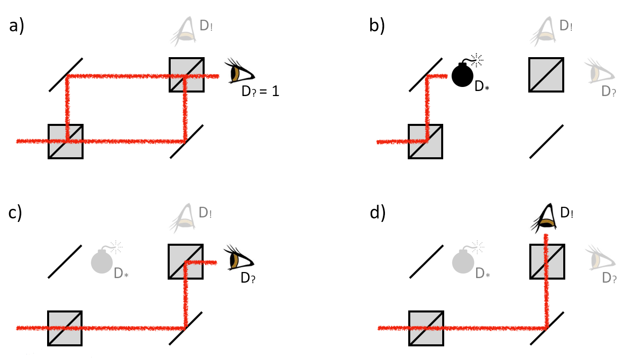
Figure 1: Interaction-free measurement and the relevant parameters. A tuned Mach-Zehnder interferometer, as in panel (a), is moved to the location where there might be a bomb in the upper arm. The probe particle triggers the bomb, single-particle-sensitive detector $D_{*}$, via path (b) with probability $P_{*}$. The measurement is inconclusive if the particle takes path (c) because the detector labeled $D_{?}$ also fires when there is no bomb, see (a). The probability of an inconclusive result is denoted by $P_{?}$. Finally, the measurement succeeds if the top detector clicks and this happens with probability $P_{!}$, see (d). The measurement is termed interaction-free, because had the particle interacted with the bomb, it would trigger it, and it did not.

I.1 Perfect interaction-free measurement

We call an interaction-free measurement perfect when statistics of single-shot experiments with the same interferometer shows

$$P_{*}=0\quad\textrm{ and }\quad P_{?}<1,$$ (2)

i.e., when the bomb never explodes, and yet from time to time, we are certain it was there. The paper ends with an example where both of these probabilities are zero.

It should be emphasized that this definition involves only probabilities in certain experimental scenarios and hence it is independent of the underlying physical theory. Now we show that a broad class of physical models, including quantum mechanics, does not permit perfect interaction-free measurements.

I.2 No perfect interaction-free measurements in amplitude models

In quantum mechanics, the condition $P_{*}=0$ implies a vanishing probability amplitude for the particle to propagate along the path of the bomb. This means that the first (generalized) beam splitter never sends the particle to that path and hence it is irrelevant whether one places a bomb there or not, i.e., $P_{?}=1$. The same conclusion holds in any theory that assigns probability amplitudes to physical processes and demands that the vanishing probability of the process implies a vanishing amplitude, e.g., the probability is an arbitrary power of the amplitude. It is intriguing in the present context that many of such models do not give rise to multipath coherence. If the amplitudes are complex numbers (or even pairs of real numbers), their natural composition laws lead to Feynman rules, i.e. probability $\sim$ amplitude² IntJThPhys.27.543 ; PRA.81.022109 . Sorkin’s original argument then demonstrates the absence of multi-path interference ModPhysLettA.9.3119 .

This elementary argument excludes the possibility of perfect interaction-free measurements in quantum mechanics. We therefore ask to what extent are such measurements forbidden. The answer is phrased as a trade-off relation between the probability of detonation and the probability of an inconclusive result. It shows that the inconclusive result happens more and more often with a decreasing probability of triggering the bomb.

I.3 Quantum trade-off

Figure 2: A general interferometer used to derive the trade-off relations. The particle is injected into the first path from the left. It enters the interferometer via transformation $\mathcal{T}_{1}$ and leaves it via transformation $\mathcal{T}_{2}$. Inside the interferometer the bomb is present in the first path.

Consider a general interferometer as shown in Fig. 2. We present the trade-off between $P_{*}$ and $P_{?}$ for arbitrary mixed quantum states but keeping the second transformation unitary, i.e. $\mathcal{T}_{2}=\mathcal{U}_{2}$. Let us denote by $\rho$ the density matrix of the particle inside the interferometer, right after the first transformation. The probability to trigger the bomb is given by

$$P_{*}=\left\langle 1\right|\rho\left|1\right\rangle.$$ (3)

If the bomb is not triggered, the state $\rho$ gets updated to $\tilde{\rho}$ satisfying:

$$\tilde{\rho}=\frac{1}{1-P_{*}}(\mathds{1}-\left|1\right\rangle\left\langle 1\right|)\rho(\mathds{1}-\left|1\right\rangle\left\langle 1\right|),$$ (4)

where $\mathds{1}$ is the identity operator in the space of density matrices. Accordingly, the particle at the output of the interferometer is described by $\mathcal{U}_{2}\,\tilde{\rho}\,\mathcal{U}_{2}^{\dagger}$. The probability of an inconclusive result is given by the chance that now the particle is observed at those output ports $\left|s\right\rangle$ in which it might be present if there was no bomb:

$$P_{?}=(1-P_{*})\sum_{s}\left\langle s\right|\mathcal{U}_{2}\,\tilde{\rho}\,\mathcal{U}_{2}^{\dagger}\left|s\right\rangle,$$ (5)

where we multiplied by $(1-P_{*})$ to account for the renormalisation in $\tilde{\rho}$. In Appendix A we derive the following trade-off relation:

$$P_{?} \geq 1-2P_{*}+P_{*}\left\langle 1\right|E(\rho)\left|1\right\rangle$$ (6)

$$\geq (1-P_{*})^{2},$$

where $E(\rho)$ is the projector on the support of $\rho$, i.e. $E(\rho)=\sum_{r}\left|r\right\rangle\left\langle r\right|$ for $\rho=\sum_{r}p_{r}\left|r\right\rangle\left\langle r\right|$. The last inequality in (6) follows from convexity, $\left\langle 1\right|E(\rho)\left|1\right\rangle\geq\left\langle 1\right|\rho\left|1\right\rangle$. We now discuss special cases of this trade-off in order to illustrate the tightness of the bound and for future comparison with the model of density cubes.

First of all, due to convexity, the lower bound is saturated by pure states. In other words, pure states are the best for interaction-free measurements. Note also that in quantum formalism, by starting with a pure state $\rho$ one always obtains a pure state $\tilde{\rho}$ after the measurement. It turns out that the cube model does not share this property.

Any density matrix $\rho$ that does not contain coherence to the state $\left|1\right\rangle$, i.e. has vanishing off-diagonal elements in the first row and column when $\rho$ is written in a basis including $\left|1\right\rangle$, is useless for interaction-free measurements. If there is no coherence to state $\left|1\right\rangle$, then either (i) one of the eigenvectors of $\rho$ is this state or (ii) all the eigenvectors are orthogonal to $\left|1\right\rangle$. In the case (i) we find $\left\langle 1\right|E(\rho)\left|1\right\rangle=1$ and hence:

$$P_{?}\geq 1-P_{*}.$$ (7)

This combined with the normalisation condition (1), means that there is no place for a successful interaction-free measurement, i.e. $P_{!}=0$. In the case (ii) we note that $P_{*}=0$ and hence the lower bound in (6) already shows that $P_{?}=1$. This demonstrates quantitatively the impossibility of perfect interaction-free measurements. Finally, we note that the trade-off just derived holds for an arbitrary interferometer (with the second transformation being unitary) and that it is independent of the number of paths. For example, the inequality (6) is saturated by taking the discrete Fourier transform as both transformations in the interferometer with an arbitrary number of paths. This again will differ in the density cube model.

II Density cubes

The trade-off relation just derived captures the impossibility of perfect interaction-free measurement in the quantum formalism. We show here that their absence is a natural postulate which disqualifies certain extensions of quantum mechanics, namely, the density cube model NJP.16.023028 . This model has been introduced in order to incorporate the possibility of multipath coherence, and we shall first say a few words about where exactly could such an extension show up in an experiment. Sorkin introduced the following classification ModPhysLettA.9.3119 . Quantum mechanics gives rise to second-order interference because the interference pattern observed on the screen behind two open slits, I12, cannot be understood as a simple sum of patterns when each individual slit is closed, i.e., $I_{12}-I_{1}-I_{2}\neq 0$. However, the interference fringes observed in a triple-slit experiment are always reducible to a simple combination of double-slit and single-slit patterns, namely, $I_{123}=I_{12}+I_{13}+I_{23}-I_{1}-I_{2}-I_{3}$. Similar statements hold for higher numbers of slits. Why does quantum mechanics “stop” at second-order interference? How would a model that gives rise to third-order and higher-order interference look? The density cube formalism provides the answer to the latter question. In principle it could show up in triple-slit experiments. However, the present paper finds that this is unlikely because the cubes allow for perfect interaction-free measurements.

In order to keep the present work self-contained, we first review the elements of the cubes model.We then derive the trade-off relation between $P_{?}$ and $P_{*}$ within the density cubes framework, which hints at the possibility of perfect interaction-free measurement. Finally, we provide explicit examples of such measurements.

II.1 Probability

The main difference between quantum mechanics and the cubes framework is that instead of a density matrix, one assigns a rank-$3$ tensor (density cube) to a given physical configuration. The density cube $C$ can have complex elements $C_{jkl}\in\mathbb{C}$. The density cubes are assumed to be Hermitian in the sense that exchanging two indices produces a complex conjugated element, e.g.,

$$C_{jkl}=C_{kjl}^{*}.$$ (8)

Hermitian cubes form a real vector space with inner product

$$(M,C)=\sum_{j,k,l=1}^{N}M_{jkl}^{*}C_{jkl},$$ (9)

where each index of the tensor runs through values $1,\dots,N$. Therefore, one naturally defines the probability of observing an outcome corresponding to cube $M$ in a measurement on a physical object described by cube $C$ by the above inner product. This is in close analogy to the Born rule in quantum mechanics, which in the same situation assigns probability $\mathrm{Tr}(MC)=\sum_{j,k=1}^{N}M_{jk}^{*}C_{jk}$, with $M$ and $C$ being density matrices. In this way the model of the density cubes extends the self-duality between states and measurements present in quantum mechanics NJP.12.033034 ; 1110.6607 .

II.2 States

We shall consider two types of density cubes: the quantum cubes which represent quantum states in the density cube model and nonquantum cubes (with triple-path coherence) that extend the quantum set. The former are constructed from quantum states and are in one-to-one relationwith the quantum states. While nonquantum cubes are also constructed starting from a quantum state, one can choose various combinations for the triple-path coherence terms to construct several distinct nonquantum cubes corresponding to a given quantum state.

The sets of allowed density cubes and their transformations are not yet fully characterized and it is not our aim to characterize them in this paper. We will rather focus on specific density cubes and transformations, which will be shown to be consistent and will produce perfect interaction-free measurements.

II.2.1 Quantum cubes

Consider the following mapping between a density matrix $\rho$ and a cube $C^{Q}$:

$$\begin{array}[]{rclcl}C_{jjj}^{Q}&=&\rho_{jj},&&\\ C_{jjk}^{Q}&=&\sqrt{\frac{2}{3}}\,\textrm{Re}(\rho_{jk}),&\textrm{ for }&j<k,\\ C_{jkk}^{Q}&=&\sqrt{\frac{2}{3}}\,\textrm{Im}(\rho_{jk}),&\textrm{ for }&j<k,\\ C_{jkl}^{Q}&=&0,&\textrm{ for }&j\neq k\neq l.\end{array}$$ (10)

Note that all the terms $C_{jkl}^{Q}$ where the three indices are different are set to zero, meaning that these cubes do not admit any three-path coherence. The remaining elements can be computed using the Hermiticity rule. This mapping preserves the inner product between the states, and hence quantum mechanics and the density cube model with this set of cubes are physically equivalent.

II.2.2 Non-quantum cubes

We now extend the set of quantum cubes and allow for non-trivial triple-path coherence by mapping every quantum state $\rho$ to the following family of cubes:

$$C_{jjj} = \frac{1}{N-1}(1-\rho_{jj}),$$

$$C_{jjk} = \sqrt{\frac{2}{3}}\frac{1}{N-1}\,\textrm{Re}(\rho_{jk}),\quad\textrm{ for }\quad j<k,$$

$$C_{jkk} = \sqrt{\frac{2}{3}}\frac{1}{N-1}\,\textrm{Im}(\rho_{jk}),\quad\textrm{ for }\quad j<k,$$

$$C_{1jk}(\gamma) = \sqrt{\frac{1}{3}}\frac{1}{N-1}\,\omega^{f(\gamma,j,k)},\quad\textrm{ for }\quad 1<j<k,$$

where $\omega=\exp(-i2\pi/N)$ is the $N$th complex root of unity and $f(\gamma,j,k)=\{1,\dots,N\}$. The parameter $\gamma=1,\dots,N$ enumerates different cubes that can be constructed from a given quantum state. Again, the remaining elements can be completed using the Hermiticity rule. We provide explicit examples of interesting non-quantum cubes in Sec. II.5 and Appendix C. Note that for simplicity we choose to place the bomb in the first path of the interferometer and therefore consider cubes where the three-path coherence involves only the first path (labeled by index $1$) and two other paths. All the terms $C_{jkl}$, with three different indices, each of which is strictly greater than $1$, are set to zero.

II.3 Measurement

We shall only be interested in enquiring about the particle’s path at various stages of the evolution. Furthermore, we will focus on checking whether the particle is in the first path or not. Clearly this measurement is allowed in quantum mechanics, and we choose vector $(1\,0\,0)^{T}$ to represent the particle moving along the first (out of three) paths inside the interferometer. The corresponding quantum cube looks as follows, see Eq. (10), in the case of the triple-path experiment:

$$M_{1} = \left\{\left(\begin{array}[]{ccc}1&0&0\\ 0&0&0\\ 0&0&0\end{array}\right),\left(\begin{array}[]{ccc}0&0&0\\ 0&0&0\\ 0&0&0\end{array}\right),\left(\begin{array}[]{ccc}0&0&0\\ 0&0&0\\ 0&0&0\end{array}\right)\right\},$$ (21)

where the three $3\times 3$ matrices describing the cube have elements $C_{1jk}$, $C_{2jk}$ and $C_{3jk}$, respectively. The probability that a particle described by cube $C$ is found in the first path is $(M_{1},C)$.

It is essential to the interaction-free measurement to describe the state of the particle after it has not been found in a particular path. Here the model of density cubes follows quantum mechanics and it is assumed that the cube describing the system changes as a result of measurement. If the particle is found in the $n$th path, its state gets updated $C\to M_{n}$, where $M_{n}$ is the quantum cube corresponding to a particle propagating along the $n$th path. If the particle is not found in the $n$th path, the model follows the generalized Lüder’s state update rule: it erases from the cube all elements $C_{jkl}$ with $j,k,l=n$, and renormalizes the remaining elements. Following our three-path example, if the particle is not found in the first path its generic cube $C$ gets updated to cube $\tilde{C}$ with elements

$$\left\{\left(\begin{array}[]{ccc}0&0&0\\ 0&0&0\\ 0&0&0\end{array}\right),\left(\begin{array}[]{ccc}0&0&0\\ 0&\tilde{C}_{222}&\tilde{C}_{223}\\ 0&\tilde{C}_{232}&\tilde{C}_{233}\end{array}\right),\left(\begin{array}[]{ccc}0&0&0\\ 0&\tilde{C}_{322}&\tilde{C}_{323}\\ 0&\tilde{C}_{332}&\tilde{C}_{333}\end{array}\right)\right\},$$ (32)

(33)

where

$$\tilde{C}_{jkl}=\frac{1}{1-C_{111}}C_{jkl},$$ (34)

is the cube element renormalised by the probability that the particle is not in the first path.

At this stage we must ensure that all postmeasurement cubes are allowed within the model. This is immediately clear if one begins with a quantum cube. For the nonquantum cubes we note that we only consider those cubes which have three-path coherence to the first path and we only enquire whether the particle is in the first path or not. If the measurement does not find the particle in the first path, all these coherences are updated to zero and accordingly, the postmeasurement cube is a quantum one.

II.4 Cubes trade-off

We are now ready to present the trade-off relation between $P_{*}$ and $P_{?}$ for a general interferometer in Fig. 2. Our trade-off relation holds for the transformation $\mathcal{T}_{2}$ that preserves the inner product, while having an additional assumption on the structure of the cube $C$ describing the particle inside the interferometer right after $\mathcal{T}_{1}$. We assume that after the particle has propagated through the whole interferometer in the case of no bomb, the cube at the output does not have any two-path and three-path coherence:

$$\mathcal{T}_{2}(C)=\sum_{s}p_{s}M_{s}.$$ (35)

We ensure this is always fulfilled in our examples. Similarly to the quantum case, the probabilities entering the trade-off are defined as follows:

$$P_{*} = (M_{1},C),$$

$$P_{?} = (1-P_{*})\sum_{s}(M_{s},\mathcal{T}_{2}(\tilde{C})),$$ (36)

where the cube $\tilde{C}$ represents the particle inside the interferometer after the measurement in the first path has not found the particle there [see Eq. (33)]. In Appendix B we derive the trade-off relation within the cubes model:

$$P_{?}\geq\frac{(1-P_{*})^{2}}{N-1}.$$ (37)

It is illustrated in Fig. 3. One recognises that for $N=2$ this relation reduces to the one derived in quantum mechanics. For two-path interferometers this is not surprising as in this case the density cube model reduces to standard quantum formalism NJP.16.023028 . For a higher number of paths, this relation emphasizes that independence of the number of paths is a special quantum feature.

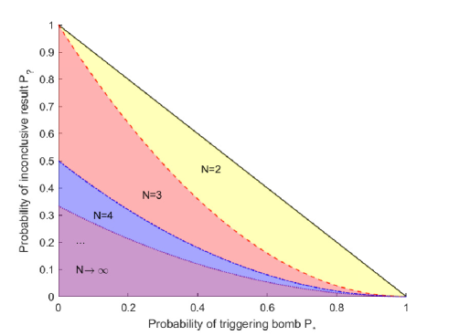
Figure 3: Trade-off between the probability to trigger the bomb $P_{*}$ and the probability of an inconclusive result $P_{?}$ within the cubes model and quantum mechanics. The straight line illustrates the trivial bound $P_{*}+P_{?}=1$. All other region borders give lower bounds on the value of $P_{?}$ as a function of $P_{*}$. The available region for any $N$ (number of paths inside the interferometer) contains also the regions for all lower values of $N$. The quantum trade-off coincides with the case of $N=2$. Perfect interaction-free measurements occur if the allowed values on the vertical axis are less than $1$.

Relation (37) opens up the possibility of perfect interaction-free measurements. Indeed, for all $N\geq 3$ one finds that the right-hand side is strictly less than 1 even if $P_{*}=0$. Furthermore, both probabilities $P_{*}$ and $P_{?}$ can in principle be brought to zero in the limit $N\to\infty$. In the next section we provide explicit examples of perfect interaction-free measurements which achieve the lower bound set by the trade-off relation (37).

II.5 Examples of perfect interaction-free measurements

We present in detail the workings of the perfect interaction-free measurement in the case of a three-path interferometer with emphasis on the features departing from the quantum formalism. The subsequent section provides the generalization to $N$ paths. We discuss the main idea here and refer to Appendix D for the details.

II.5.1 Three paths

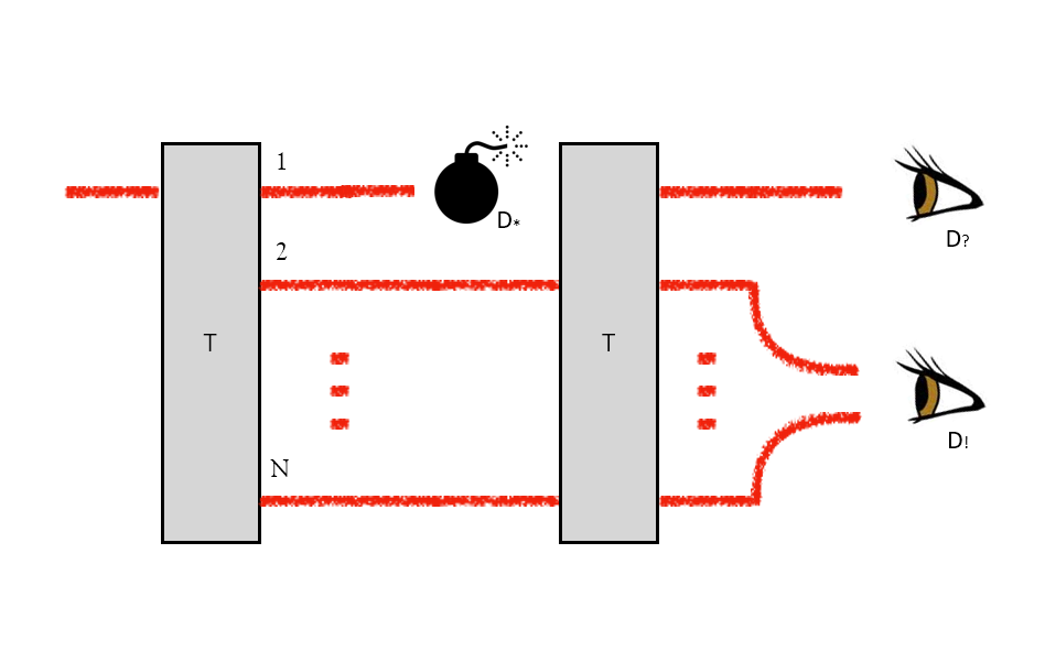
Figure 4: A perfect interaction-free measurement within the density cube model. Both transformations are the same and they have the property that $\mathcal{T}^{2}=\mathds{1}$. Therefore, if there is no bomb the particle which enters through the first path always leaves the interferometer along the first path. The cube describing the particle inside the interferometer has only triple-path coherences to the first path and yet vanishing element $C_{111}$. Therefore the particle is never found along the first path inside the interferometer and the bomb never detonates, $P_{*}=0$. However, the presence of the bomb removes the triple-path coherences from the cube. In this case, the second transformation evolves the particle to the first output port only with probability $P_{?}=\frac{1}{2}$. See main text for details.

Consider the setup described in Fig. 4. The transformation $\mathcal{T}_{1}=\mathcal{T}_{2}=\mathcal{T}\circ\mathcal{D}$ is chosen to consist of (quantum mechanical) complete dephasing of two-path coherences, $\mathcal{D}$, followed by the transformation $\mathcal{T}$ defined in Eq. (16) of Ref. NJP.16.023028 , which we will here review for completeness. The reason behind this composition of operations is that $\mathcal{T}$ is only defined on a subset of cubes and it might be that it is impossible to extend it consistently to the whole set of cubes. The role of the dephasing is then to bring an arbitrary cube to the subset on which $\mathcal{T}$ is known to act consistently. The dephasing operation is defined to remove completely all two-path coherences in a cube and leave unaffected the diagonal elements $C_{nnn}$ and triple-path coherences $C_{jkl}$ with all indices different. Since this operation acts only on the quantum part of the cube it produces allowed cubes. Transformation $\mathcal{T}$ has matrix representation

$$\mathcal{T}=\frac{1}{2}\left(\begin{array}[]{ccccc}0&1&1&1&1\\ 1&0&1&\omega^{*}&\omega\\ 1&1&0&\omega&\omega^{*}\\ 1&\omega&\omega^{*}&1&0\\ 1&\omega^{*}&\omega&0&1\end{array}\right),$$ (38)

when written in the following sub-basis of Hermitian cubes:

$$B_{1} = M_{1},\qquad B_{2}=M_{2},\qquad B_{3}=M_{3},$$

$$B_{4} = \frac{1}{\sqrt{3}}\left\{\left(\begin{array}[]{ccc}0&0&0\\ 0&0&1\\ 0&0&0\end{array}\right),\left(\begin{array}[]{ccc}0&0&0\\ 0&0&0\\ 1&0&0\end{array}\right),\left(\begin{array}[]{ccc}0&1&0\\ 0&0&0\\ 0&0&0\end{array}\right)\right\},$$ (48)

$$B_{5} = \frac{1}{\sqrt{3}}\left\{\left(\begin{array}[]{ccc}0&0&0\\ 0&0&0\\ 0&1&0\end{array}\right),\left(\begin{array}[]{ccc}0&0&1\\ 0&0&0\\ 0&0&0\end{array}\right),\left(\begin{array}[]{ccc}0&0&0\\ 1&0&0\\ 0&0&0\end{array}\right)\right\}.$$ (58)

That is, given an arbitrary cube $C$ in this subspace, the transformation $\mathcal{T}$ acts upon it via ordinary matrix multiplication on the vector representation of $C$, i.e., a five-dimensional column vector with $j$th component given by $(C,B_{j})$. As already alluded to, this subspace consists of cubes which have no two-path coherences but solely three-path coherences and diagonal terms. It is now straightforward to verify that $\mathcal{T}$ is an involution in the considered subspace, i.e. $\mathcal{T}^{2}=\mathds{1}$. Accordingly, if the particle enters the interferometer through the first path, it is always found in the first output port of the setup. This adheres to our assumption (35) as the output cube is simply $M_{1}$. The transformation T is different from an arbitrary unitary transformation as it produces triple-path coherence inside the interferometer. The particle injected into the first path is described by the cube $M_{1}$, which in the considered subspace corresponds to the vector $(1\,0\,0\,0\,0)^{T}$, and one can verify that the corresponding cube after application of $\mathcal{T}$ is $\mathcal{T}(M_{1})=\frac{1}{2}(B_{2}+B_{3}+B_{4}+B_{5})=C$, which is also given by

$$\frac{1}{2}\left\{\left(\begin{array}[]{ccc}0&0&0\\ 0&0&\frac{1}{\sqrt{3}}\\ 0&\frac{1}{\sqrt{3}}&0\end{array}\right),\left(\begin{array}[]{ccc}0&0&\frac{1}{\sqrt{3}}\\ 0&1&0\\ \frac{1}{\sqrt{3}}&0&0\end{array}\right),\left(\begin{array}[]{ccc}0&\frac{1}{\sqrt{3}}&0\\ \frac{1}{\sqrt{3}}&0&0\\ 0&0&1\end{array}\right)\right\}.$$ (60)

Note that it is a pure cube, i.e., $(C,C)=1$, and it contains solely three-path coherences and elements $C_{222}$ and $C_{333}$. The essential feature we are utilizing for perfect interaction-free measurement is the presence of these coherences even though the probability to find the particle in the first path vanishes:

$$P_{*}=(M_{1},C)=0.$$ (61)

A similar statement for quantum states does not hold. If the probability to locate a quantum particle in the first path vanishes, all coherences to this path must vanish, as otherwise the corresponding density matrix has negative eigenvalues.

If the bomb is present inside the interferometer but is not triggered, the state update rule dictates erasure of all elements $C_{jkl}$ with any of $j,k,l=1$. We obtain the following cube:

$$\tilde{C}=\left\{\left(\begin{array}[]{ccc}0&0&0\\ 0&0&0\\ 0&0&0\end{array}\right),\left(\begin{array}[]{ccc}0&0&0\\ 0&\frac{1}{2}&0\\ 0&0&0\end{array}\right),\left(\begin{array}[]{ccc}0&0&0\\ 0&0&0\\ 0&0&\frac{1}{2}\end{array}\right)\right\}.$$ (62)

It contains no coherences whatsoever and it is mixed, i.e., $(\tilde{C},\tilde{C})=\frac{1}{2}$. We started with a pure cube and post-selected a mixed one. This is also not allowed within the quantum formalism, where any pure state $\left|\psi\right\rangle=\sum_{n=1}^{N}\alpha_{n}\left|n\right\rangle$ gets updated to another pure state $|\tilde{\psi}\rangle=\sum_{n=2}^{N}\tilde{\alpha}_{n}\left|n\right\rangle$, with $\tilde{\alpha}_{n}=\alpha_{n}/\sqrt{1-|\alpha_{1}|^{2}}$.

Finally, we evolve $\tilde{C}=\frac{1}{2}M_{2}+\frac{1}{2}M_{3}$ through the second transformation and find that $\mathcal{T}(\tilde{C})$ is given by (dephasing has no effect here):

$$\Big{\{}\left(\begin{array}[]{ccc}\frac{1}{2}&0&0\\ 0&0&-\frac{1}{4\sqrt{3}}\\ 0&-\frac{1}{4\sqrt{3}}&0\end{array}\right) \left(\begin{array}[]{ccc}0&0&-\frac{1}{4\sqrt{3}}\\ 0&\frac{1}{4}&0\\ -\frac{1}{4\sqrt{3}}&0&0\end{array}\right),$$ ,

$$\left(\begin{array}[]{ccc}0&-\frac{1}{4\sqrt{3}}&0\\ -\frac{1}{4\sqrt{3}}&0&0\\ 0&0&\frac{1}{4}\end{array}\right)\Big{\}}.$$

The probability of an inconclusive result is given by the probability that the particle is found in the first path, as it was always there in the absence of the bomb, and therefore we find

$$P_{?}=(M_{1},\mathcal{T}(\tilde{C}))=\frac{1}{2}.$$ (65)

This probability saturates the lower bound derived in Eq. (37) for $N=3$ and hence the setup discussed is optimal.

II.5.2 More than three paths

We now generalize the above scheme to more than three paths and show that the density cube model allows for perfect interaction-free measurement, which in every run provides complete information about the presence of the bomb. This holds in the limit $N\to\infty$. We shall now construct a set of $N$ pure orthonormal cubes $C^{(n)}$, which will then be used to provide the transformation $\mathcal{T}$ of the optimal interferometer, that gives rise to the minimal probability of an inconclusive result while keeping $P_{*}=0$. We set the modulus of all the three-path coherences within each cube $C^{(n)}$ to be the same and choose its non-zero elements as follows:

$$C_{jjj}^{(n)} = \frac{1}{N-1},\quad\textrm{ for }j\neq n,$$

$$C_{1jk}^{(n)} = \sqrt{\frac{1}{3}}\frac{1}{N-1}\,x_{jk}^{(n)},\quad\textrm{ for }1<j<k.$$ (66)

The other non-zero three-path coherences can be found from the Hermiticity rule. In this way cube $C^{(n)}$ is represented by a set of phases $x_{jk}^{(n)}$. We arrange the independent phases, i.e. the ones having $j<k$, into a vector $\vec{x}_{n}$. The orthonormality conditions between the cubes are now expressed in the following equations

$$(C^{(n)},C^{(n)})=1\iff |(\vec{x}_{n})_{j}|=1$$

$$\textrm{ for all }n,j,$$

$$(C^{(m)},C^{(n)})=0\iff (\vec{x}_{m},\vec{x}_{n})+(\vec{x}_{n},\vec{x}_{m})=2-N,$$

$$\textrm{ for all }m\neq n.$$ (67)

where $(\vec{x}_{n})_{j}$ is the $j$th component of the vector $\vec{x}_{n}$. Equations (67) are solved in Appendix C. Let us write the solution in form of a matrix

$$X=(\vec{x}_{1}\dots\vec{x}_{N}),$$ (68)

having vectors $\vec{x}_{n}$ as columns. We now show how to use it to construct the “cube multiport” transformation $\mathcal{T}$.

We assume the two transformations in the setup are the same and that $\mathcal{T}$ is defined solely on the subspace of Hermitian cubes which do not have any two-path coherences. The cubes forming the basis set for this subspace are as follows:

$$B_{jkl}^{(n)}= \delta_{jn}\delta_{kn}\delta_{ln},\quad\textrm{ for }n=1,\dots,N$$ (69)

$$B^{(vw)}_{jkl}= \frac{1}{\sqrt{3}}\left(\delta_{j1}\delta_{kv}\delta_{lw}+\delta_{jw}\delta_{k1}\delta_{lv}+\delta_{jv}\delta_{kw}\delta_{l1}\right),$$ (70)

$$\textrm{ for }1<v<w\leq N,$$

$$B^{(wv)}_{jkl}= \frac{1}{\sqrt{3}}\left(\delta_{j1}\delta_{kw}\delta_{lv}+\delta_{jv}\delta_{k1}\delta_{lw}+\delta_{jw}\delta_{kv}\delta_{l1}\right),$$ (71)

$$\textrm{ for }1<v<w\leq N.$$

One recognizes that the cubes in the first line are just the $M_{n}$ cubes describing the particle propagating along the $n$th path. The cubes in the second line describe independent three-path coherences, and the cubes in the third line their complex conjugates. Altogether there are $d=N+(N-1)(N-2)$ cubes in this sub-basis, and hence the transformation $\mathcal{T}$ is represented by a $d\times d$ matrix, which we then divide into blocks:

$$\mathcal{T}=\left(\begin{array}[]{c|c}A&C\\ \hline\cr B&D\end{array}\right),$$ (72)

$A$ being a square $N\times N$ matrix, $D$ being a square matrix with dimension $(N-1)(N-2)\times(N-1)(N-2)$, and $B$ and $C$ being rectangular. By imposing $\mathcal{T}(M_{n})=C^{(n)}$, matrices $A$ and $B$ are fixed to

$$A=\frac{1}{N-1}\left(\begin{array}[]{cccc}0&1&\cdots&1\\ 1&0&\cdots&1\\ \vdots&\vdots&\ddots&\vdots\\ 1&1&\cdots&0\\ \end{array}\right),\qquad B=\left(\begin{array}[]{c}X\\ X^{*}\end{array}\right).$$ (73)

By further requiring involution $\mathcal{T}^{2}=\mathds{1}$ and Hermiticity $\mathcal{T}=\mathcal{T}^{\dagger}$ one finds that

$$C=B^{\dagger},\qquad D=\sqrt{\mathds{1}-BB^{\dagger}}.$$ (74)

We show in Appendix D that $\mathds{1}-BB^{\dagger}$ is a positive matrix, which concludes our construction of $\mathcal{T}$. It turns out that this is not the only way to construct the cube multiport transformation and Appendix D provides other examples. All of them transform the quantum cubes $M_{n}$ to the nonquantum cubes $C^{(n)}$. Note that in the considered subspace $M_{n}$ are the only pure quantum cubes, and one verifies that $C^{(n)}$ are the only pure nonquantum cubes allowed. In this way $\mathcal{T}$ is shown to act consistently, i.e., map cubes allowed within the model to other allowed cubes.

III Conclusions

We proposed a theory-independent definition of perfect interaction-free measurement. It turns out that quantum mechanics does not allow this possibility, which we show by an elementary argument and by a quantitative relation. However, it can be realized within the framework of density cubes NJP.16.023028 . This framework allows transformations that prepare triple-path coherence involving a path where the probability of detecting the particle is strictly zero. Nevertheless, this coherence can be destroyed if the bomb (detector) is in the setup, leading to a distinguishable outcome in a suitable one-shot interference experiment. We emphasize that, in this paper, we study single-shot experiments in contrast to the quantum Zeno effect where the interferometer is used multiple times PhysRevLett.74.4763 ; PhysRevA.90.042109 .

We postulate that perfect interaction-free measurements should not be present in a physical theory as they effectively allow deduction of the presence of an object in a particular location without ever detecting a particle in that location. One might also try to identify more elementary principles which imply the impossibility of perfect interaction-free measurements.

In this context, we note that perfect interaction-free measurements are consistent with the no-signaling principle (no superluminar communication). In the density cube model it is the triple-path coherence that is being destroyed by the presence of the detector inside the interferometer. The statistics of any observable measured on the remaining paths is the same, independently of whether the detector is in the setup or not. Hence the information about its presence can only be acquired after recombining the paths together, which can be done at most at the speed of light. The situation resembles that of the stronger-than-quantum correlations satisfying the principle of no-signaling PR . They are considered “too strong,” as they trivialize communication complexity vanDam ; PhysRevLett.96.250401 or random access coding ic , and they are at variance with many natural postulates ic ; ML ; NJP.14.063024 . Similarly, we consider identifying the presence of a detector without ever triggering it, i.e., a perfect interaction-free measurement, as too powerful to be realized in nature. Exactly which physical principles forbid such measurements is, of course, an interesting question.

Finally, we wish to comment briefly on experimental tests of genuine multipath interference. They are often described as simultaneously testing the validity of Born’s rule. Indeed, as we pointed out here, this is the case for a broad class of models which assign probability amplitudes to physical processes and these amplitudes satisfy natural composition laws IntJThPhys.27.543 ; PRA.81.022109 . Other models, however, are possible, as exemplified by the density cube framework. Within this framework the probability rule is essentially the same as the Born rule in quantum mechanics. [For its version for mixed states, see Eq. (9).] Therefore, in general, tests of multipath interference should be distinguished from validity tests of Born’s rule.

Appendix A Proof of the quantum trade-off

Let us denote the eigenstates of the density matrix $\rho$ describing the particle inside the interferometer right after the first transformation as $\left|r\right\rangle$, i.e., $\rho=\sum_{r}p_{r}\left|r\right\rangle\left\langle r\right|$. We also write $\mathcal{U}_{2}\left|r\right\rangle=\left|\phi_{r}\right\rangle$. From the definition of the probability of an inconclusive result,

$$\frac{P_{?}}{1-P_{*}}=\mathrm{Tr}\left(\sum_{s}\left|s\right\rangle\left\langle s\right|\mathcal{U}_{2}\,\tilde{\rho}\,\mathcal{U}_{2}^{\dagger}\right),$$ (75)

where the sum is over the paths $\left|s\right\rangle$ at the output of the interferometer where the particle could be found if there was no bomb, i.e., if $\mathcal{U}_{2}\,\rho\,\mathcal{U}_{2}^{\dagger}=\sum_{r}p_{r}\left|\phi_{r}\right\rangle\left\langle\phi_{r}\right|$ is the state at the output. Therefore, states $\left|s\right\rangle$ span a subspace that contains the eigenstates $\left|\phi_{r}\right\rangle$ and we conclude that,

$$\sum_{s}\left|s\right\rangle\left\langle s\right|=\sum_{r}\left|\phi_{r}\right\rangle\left\langle\phi_{r}\right|+\sum_{\mu}\left|\mu\right\rangle\left\langle\mu\right|,$$ (76)

where the $\left|\mu\right\rangle$’s complement the subspace spanned by the paths. Since $\left\langle\mu\right|\mathcal{U}_{2}\,\tilde{\rho}\,\mathcal{U}_{2}^{\dagger}\left|\mu\right\rangle\geq 0$, Eq. (75) admits the lower bound:

$$\frac{P_{?}}{1-P_{*}}\geq\mathrm{Tr}\left(\sum_{r}\left|\phi_{r}\right\rangle\left\langle\phi_{r}\right|\mathcal{U}_{2}\,\tilde{\rho}\,\mathcal{U}_{2}^{\dagger}\right)=\mathrm{Tr}\left(\sum_{r}\left|r\right\rangle\left\langle r\right|\tilde{\rho}\right).$$ (77)

Using the definition of $\tilde{\rho}$ in terms of $\rho$ given in Eq. (4) of the main text we obtain

$$P_{?}\geq 1-2P_{*}+P_{*}\left\langle 1\right|E(\rho)\left|1\right\rangle,$$ (78)

with $E(\rho)=\sum_{r}\left|r\right\rangle\left\langle r\right|$.

Appendix B Proof of the cubes trade-off

Let us first recall our assumption about cube $C$ describing the particle inside the interferometer [Eq. (35) of the main text]:

$$\mathcal{T}_{2}(C)=\sum_{s}p_{s}M_{s}.$$ (79)

The following steps form the first part of the derivation:

$$\frac{P_{?}}{1-P_{*}} =\sum_{s}(M_{s},\mathcal{T}_{2}(\tilde{C}))$$

$$\geq\sum_{s}(p_{s}M_{s},\mathcal{T}_{2}(\tilde{C}))$$

$$=(\mathcal{T}_{2}(C),\mathcal{T}_{2}(\tilde{C}))=(C,\tilde{C}).$$ (80)

The first line is the definition of the probability of an inconclusive result, the inequality follows from convexity, and then we used (79) and finally the fact that $\mathcal{T}_{2}$ preserves the inner product. In the second part we shall find the minimum of the right-hand side. Using the expression for the elements of $\tilde{C}$ in terms of the elements of $C$ we find:

$$(C,\tilde{C})=\frac{1}{1-P_{*}}\sum_{j,k,l=2}^{N}|C_{jkl}|^{2},$$ (81)

where $C_{222}+\dots+C_{NNN}=1-P_{*}$. Since all of the summands are non-negative, we get the lower bound by setting all the off-diagonal terms to zero. It is then easy to verify that the minimum is achieved for an even distribution of the probability:

$$C_{nnn}=\frac{1-P_{*}}{N-1}\quad\textrm{ for }n=2,\dots,N.$$ (82)

Using this lower bound in (80) we obtain

$$P_{?}\geq\frac{(1-P_{*})^{2}}{N-1}.$$ (83)

Appendix C Solution to the orthonormality equations for optimal cubes

The solution is divided into two parts: $N$ even and $N$ odd.

C.1 $N$ even

Let $M$ be a $(N-1)\times N$ matrix formed from the discrete $N\times N$ Fourier transform by deleting the first row:

$$M=\left(\begin{array}[]{ccccc}1&\omega^{1\cdot 1}&\omega^{1\cdot 2}&\cdots&\omega^{1\cdot(N-1)}\\ 1&\omega^{2\cdot 1}&\omega^{2\cdot 2}&\cdots&\omega^{2\cdot(N-1)}\\ \vdots&\vdots&\vdots&\ddots&\vdots\\ 1&\omega^{(N-1)\cdot 1}&\omega^{(N-1)\cdot 2}&\cdots&\omega^{(N-1)\cdot(N-1)}\end{array}\right),$$ (84)

where $\omega=\exp(i2\pi/N)$. The crucial property we shall use is expressed in the following multiplication:

$$M^{\dagger}M=\left(\begin{array}[]{cccc}N-1&-1&\cdots&-1\\ -1&N-1&\cdots&-1\\ \vdots&\vdots&\ddots&\vdots\\ -1&-1&\cdots&N-1\\ \end{array}\right).$$ (85)

Hence, the columns of matrix $M$ form vectors with fixed overlap equal to $-1$, for any pair of distinct vectors. Let us now form the matrix $X$ by stacking $(N-2)/2$ matrices $M$ vertically:

$$X=\left(\begin{array}[]{c}M\\ M\\ \vdots\\ M\end{array}\right).$$ (86)

Note that matrix $X$ has $N$ columns and $(N-1)(N-2)/2$ rows. We therefore define vectors $\vec{x}_{n}$ as columns of $X$:

$$X=\left(\begin{array}[]{cccc}\vec{x}_{1}&\vec{x}_{2}&\cdots&\vec{x}_{N}\end{array}\right).$$ (87)

Indeed, every component of each $\vec{x}_{n}$ has unit modulus and appropriate overlap:

$$(\vec{x}_{m},\vec{x}_{n})+(\vec{x}_{n},\vec{x}_{m})=2(\vec{x}_{m},\vec{x}_{n})$$

$$=2(m\textrm{th row of }X^{\dagger})(n\textrm{th row of }X)$$

$$=(N-2)(m\textrm{th row of }M^{\dagger})(n\textrm{th row of }M)$$

$$=2-N.$$ (88)

C.2 $N$ odd

We now construct the matrix $M$, having dimensions $\frac{N-1}{2}\times N$, by deleting the first row of the $N\times N$ Fourier transform matrix and taking only the top $\frac{N-1}{2}$ rows left:

$$M=\left(\begin{array}[]{ccccc}1&\omega^{1\cdot 1}&\omega^{1\cdot 2}&\cdots&\omega^{1\cdot N}\\ 1&\omega^{1\cdot 1}&\omega^{1\cdot 2}&\cdots&\omega^{1\cdot N}\\ \vdots&\vdots&\vdots&\ddots&\vdots\\ 1&\omega^{\frac{N-1}{2}\cdot 1}&\omega^{\frac{N-1}{2}\cdot 2}&\cdots&\omega^{\frac{N-1}{2}\cdot N}\end{array}\right).$$ (89)

This time we have:

$$M^{\dagger}M=\left(\begin{array}[]{cccc}\frac{N-1}{2}&-\frac{1}{2}&\cdots&-\frac{1}{2}\\ -\frac{1}{2}&\frac{N-1}{2}&\cdots&-\frac{1}{2}\\ \vdots&\vdots&\ddots&\vdots\\ -\frac{1}{2}&-\frac{1}{2}&\cdots&\frac{N-1}{2}\\ \end{array}\right)+i\,(\textrm{imaginary part}).$$ (90)

We form the matrix $X$ by stacking $N-2$ matrices $M$ vertically and define vectors $\vec{x}_{n}$ as columns of $X$, as before. Indeed, the overlap between distinct vectors reads:

$$(\vec{x}_{m},\vec{x}_{n})+(\vec{x}_{n},\vec{x}_{m})=2\mathrm{Re}\left[(\vec{x}_{m},\vec{x}_{n})\right]$$ (91)

$$=2\mathrm{Re}\left[(m\textrm{th row of }X^{\dagger})(n\textrm{th row of }X)\right]$$

$$=2(N-2)\mathrm{Re}\left[(m\textrm{th row of }M^{\dagger})(n\textrm{th row of }M)\right]$$

$$=2-N.$$

C.3 Example of resulting cubes for $N=4$

The following four cubes are obtained for the four-path interferometer:

$$C^{(1)} = \frac{1}{3\sqrt{3}}\left\{\left(\begin{array}[]{cccc}0&0&0&0\\ 0&0&1&1\\ 0&1&0&1\\ 0&1&1&0\end{array}\right),\left(\begin{array}[]{cccc}0&0&1&1\\ 0&\sqrt{3}&0&0\\ 1&0&0&0\\ 1&0&0&0\end{array}\right),\left(\begin{array}[]{cccc}0&1&0&1\\ 1&0&0&0\\ 0&0&\sqrt{3}&0\\ 1&0&0&0\end{array}\right),\left(\begin{array}[]{cccc}0&1&1&0\\ 1&0&0&0\\ 1&0&0&0\\ 0&0&0&\sqrt{3}\end{array}\right)\right\},$$ (108)

$$C^{(2)} = \frac{1}{3\sqrt{3}}\left\{\left(\begin{array}[]{cccc}\sqrt{3}&0&0&0\\ 0&0&-i&-1\\ 0&i&0&i\\ 0&-1&-i&0\end{array}\right),\left(\begin{array}[]{cccc}0&0&i&-1\\ 0&0&0&0\\ -i&0&0&0\\ -1&0&0&0\end{array}\right),\left(\begin{array}[]{cccc}0&-i&0&i\\ i&0&0&0\\ 0&0&\sqrt{3}&0\\ -i&0&0&0\end{array}\right),\left(\begin{array}[]{cccc}0&-1&-i&0\\ -1&0&0&0\\ i&0&0&0\\ 0&0&0&\sqrt{3}\end{array}\right)\right\},$$ (125)

$$C^{(3)} = \frac{1}{3\sqrt{3}}\left\{\left(\begin{array}[]{cccc}\sqrt{3}&0&0&0\\ 0&0&-1&1\\ 0&-1&0&-1\\ 0&1&-1&0\end{array}\right),\left(\begin{array}[]{cccc}0&0&-1&1\\ 0&\sqrt{3}&0&0\\ -1&0&0&0\\ 1&0&0&0\end{array}\right),\left(\begin{array}[]{cccc}0&-1&0&-1\\ -1&0&0&0\\ 0&0&0&0\\ -1&0&0&0\end{array}\right),\left(\begin{array}[]{cccc}0&1&-1&0\\ 1&0&0&0\\ -1&0&0&0\\ 0&0&0&\sqrt{3}\end{array}\right)\right\},$$ (142)

$$C^{(4)} = \frac{1}{3\sqrt{3}}\left\{\left(\begin{array}[]{cccc}\sqrt{3}&0&0&0\\ 0&0&i&-1\\ 0&-i&0&-i\\ 0&-1&i&0\end{array}\right),\left(\begin{array}[]{cccc}0&0&-i&-1\\ 0&\sqrt{3}&0&0\\ i&0&0&0\\ -1&0&0&0\end{array}\right),\left(\begin{array}[]{cccc}0&i&0&-i\\ -i&0&0&0\\ 0&0&\sqrt{3}&0\\ i&0&0&0\end{array}\right),\left(\begin{array}[]{cccc}0&-1&i&0\\ -1&0&0&0\\ -i&0&0&0\\ 0&0&0&0\end{array}\right)\right\}.$$ (159)

Appendix D Consistency of the transformation

D.1 Positivity of matrix $D$

We shall find the eigenvalues of $\mathds{1}-BB^{\dagger}$ explicitly. Since $B=(X\,\,X^{*})^{T}$, the construction in Appendix C for even $N$ produces matrix $(N-1)^{2}BB^{\dagger}$, given by

$$\left(\begin{array}[]{c|c}\begin{array}[]{ccc}MM^{\dagger}&\cdots&MM^{\dagger}\\ \vdots&\ddots&\vdots\\ MM^{\dagger}&\cdots&MM^{\dagger}\end{array}&\begin{array}[]{ccc}M^{*}M^{\dagger}&\cdots&M^{*}M^{\dagger}\\ \vdots&\ddots&\vdots\\ M^{*}M^{\dagger}&\cdots&M^{*}M^{\dagger}\end{array}\\ \hline\cr\begin{array}[]{ccc}MM^{T}&\cdots&MM^{T}\\ \vdots&\ddots&\vdots\\ MM^{T}&\cdots&MM^{T}\end{array}&\begin{array}[]{ccc}M^{*}M^{T}&\cdots&M^{*}M^{T}\\ \vdots&\ddots&\vdots\\ M^{*}M^{T}&\cdots&M^{*}M^{T}\end{array}\end{array}\right),$$ (160)

Note that $MM^{\dagger}=N\,\mathds{1}$ is inherited from the unitarity of the Fourier matrix. Similarly, $M^{*}M^{T}=(M^{\dagger})^{T}M^{T}=(MM^{\dagger})^{T}=N\,\mathds{1}$. Direct computation shows that $MM^{T}=M^{*}M^{\dagger}=N\,\mathds{1}^{A}$, where $\mathds{1}^{A}$ denotes an antidiagonal matrix with all nonzero elements being $1$. Therefore, the matrix $(N-1)^{2}BB^{\dagger}$ has the following form for even $N$:

$$\left(\begin{array}[]{c|c}\begin{array}[]{ccccccc}1&&&&1&&\\ &\ddots&&\cdots&&\ddots&\\ &&1&&&&1\\ &\vdots&&&&\vdots&\\ 1&&&&1&&\\ &\ddots&&\cdots&&\ddots&\\ &&1&&&&1\\ \end{array}&\begin{array}[]{ccccccc}&&1&&&&1\\ &\reflectbox{$\ddots$}&&\cdots&&\reflectbox{$\ddots$}&\\ 1&&&&1&&\\ &\vdots&&&&\vdots&\\ &&1&&&&1\\ &\reflectbox{$\ddots$}&&\cdots&&\reflectbox{$\ddots$}&\\ 1&&&&1&&\\ \end{array}\\ \hline\cr\begin{array}[]{ccccccc}&&1&&&&1\\ &\reflectbox{$\ddots$}&&\cdots&&\reflectbox{$\ddots$}&\\ 1&&&&1&&\\ &\vdots&&&&\vdots&\\ &&1&&&&1\\ &\reflectbox{$\ddots$}&&\cdots&&\reflectbox{$\ddots$}&\\ 1&&&&1&&\\ \end{array}&\begin{array}[]{ccccccc}1&&&&1&&\\ &\ddots&&\cdots&&\ddots&\\ &&1&&&&1\\ &\vdots&&&&\vdots&\\ 1&&&&1&&\\ &\ddots&&\cdots&&\ddots&\\ &&1&&&&1\\ \end{array}\end{array}\right).$$ (161)

Similarly, one finds the following for odd $N$:

$$\left(\begin{array}[]{c|c}\begin{array}[]{ccccccc}1&&&&1&&\\ &\ddots&&\cdots&&\ddots&\\ &&1&&&&1\\ &\vdots&&&&\vdots&\\ 1&&&&1&&\\ &\ddots&&\cdots&&\ddots&\\ &&1&&&&1\\ \end{array}&\begin{array}[]{c}0\end{array}\\ \hline\cr\begin{array}[]{c}0\end{array}&\begin{array}[]{ccccccc}1&&&&1&&\\ &\ddots&&\cdots&&\ddots&\\ &&1&&&&1\\ &\vdots&&&&\vdots&\\ 1&&&&1&&\\ &\ddots&&\cdots&&\ddots&\\ &&1&&&&1\\ \end{array}\end{array}\right).$$ (162)

In both cases, the eigenvalues of $BB^{\dagger}$ are either $0$ or $N(N-2)/(N-1)^{2}$. Hence, the eigenvalues of $D$ are either $1$ or $1/(N-1)^{2}$.

D.2 Exemplary transformation for $N=4$

We shall only present the $D$ matrices. Following the method above one finds

$$D=\frac{1}{3}\begin{pmatrix}2&0&0&0&0&-1\\ 0&2&0&0&-1&0\\ 0&0&2&-1&0&0\\ 0&0&-1&2&0&0\\ 0&-1&0&0&2&0\\ -1&0&0&0&0&2\end{pmatrix}.$$ (163)

This is not the only solution given the constraints $\mathcal{T}^{2}=\mathds{1}$ and $\mathcal{T}=\mathcal{T}^{\dagger}$. The following two matrices were obtained by other means:

$$D_{2}=\frac{1}{3}\left(\begin{array}[]{cccccc}1&-i&i&-i&i&0\\ i&1&1&-1&0&-i\\ -i&1&1&0&-1&i\\ i&-1&0&1&1&-i\\ -i&0&-1&1&1&i\\ 0&i&-i&i&-i&1\end{array}\right),$$ (164)

$$D_{3}=\frac{1}{3}\left(\begin{array}[]{cccccc}1&-1&-i&i&1&0\\ -1&1&-i&i&0&1\\ i&i&1&0&-i&-i\\ -i&-i&0&1&i&i\\ 1&0&i&-i&1&-1\\ 0&1&i&-i&-1&1\end{array}\right).$$ (165)

If we use $D_{3}$ as an example, then $\mathcal{T}$ has the following elements:

$$\mathcal{T}=\frac{1}{3}\begin{pmatrix}0&1&1&1&1&1&1&1&1&1\\ 1&0&1&1&i&-1&-i&-i&-1&i\\ 1&1&0&1&-1&1&-1&-1&1&-1\\ 1&1&1&0&-i&-1&i&i&-1&-i\\ 1&-i&-1&i&1&-1&-i&i&1&0\\ 1&-1&1&-1&-1&1&-i&i&0&1\\ 1&i&-1&-i&i&i&1&0&-i&-i\\ 1&i&-1&-i&-i&-i&0&1&i&i\\ 1&-1&1&-1&1&0&i&-i&1&-1\\ 1&-i&-1&i&0&1&i&-i&-1&1\end{pmatrix}.$$ (166)

References

- (1) A. C. Elitzur and L. Vaidman. Quantum mechanical interaction-free measurements. Found. Phys., 23,987 (1993).
- (2) L. Vaidman. On the realisation of interaction-free measurements. Quantum Opt., 6,119 (1994).
- (3) P. Kwiat, H. Weinfurter, T. Herzog, A. Zeilinger, and M. A. Kasevich. Interaction-free measurement. Phys. Rev. Lett., 74,4763 (1995).
- (4) M. Hafner and J. Summhammer. Experiment on interaction-free measurement in neutron interferometry. Phys. Lett. A, 235,563 (1997).
- (5) T. Tsegaye, E. Goobar, A. Karlsson, G. Björk, M. Y. Loh, and K. H. Lim. Efficient interaction-free measurements in a high-finesse interferometer. Phys. Rev. A, 57,3987 (1998).
- (6) C. Robens, W. Alt, C. Emary, D. Meschede, and A. Alberti. Atomic “bomb testing”: the Elitzur–Vaidman experiment violates the Leggett–Garg inequality. Appl. Phys. B, 123,12 (2017).
- (7) X.-S. Ma, X. Guo, C. Schuck, K. Y. Fong, L. Jiang, and H. X. Tang. On-chip interaction-free measurements via the quantum Zeno effect. Phys. Rev. A, 90,042109 (2014).
- (8) G. S. Paraoanu. Interaction-free measurements with superconducting qubits. Phys. Rev. Lett., 97,180406 (2006).
- (9) W. K. Wootters and W. H. Zurek. A single quantum cannot be cloned. Nature (London), 299,802 (1982).
- (10) D. Dieks. Communication by EPR devices. Phys. Lett. A, 92,271 (1982).
- (11) H. Barnum, C. M. Caves, C. A. Fuchs, R. Jozsa, and B. Schumacher. Noncommuting mixed states cannot be broadcast. Phys. Rev. Lett., 76,2818 (1996).
- (12) M. Piani, P. Horodecki, and R. Horodecki. No-local-broadcasting theorem for multipartite quantum correlations. Phys. Rev. Lett., 100,090502 (2008).
- (13) A. K. Pati and S. L. Braunstein. Impossibility of deleting an unknown quantum state. Nature, 404,164 (2000).
- (14) B. Dakić, T. Paterek, and Č. Brukner. Density cubes and higher-order interference theories. New J. Phys., 16,023028 (2014).
- (15) R. D. Sorkin. Quantum mechanics as quantum measure theory. Mod. Phys. Lett. A, 9,3119 (1994).
- (16) C. M. Lee and J. H. Selby. Higher-order interference in extensions of quantum theory. Found. Phys., 47,89 (2017).
- (17) U. Sinha, C. Couteau, T. Jennewein, R. Laflamme, and G. Weihs. Ruling out multi-order interference in quantum mechanics. Science, 329,418 (2010).
- (18) I. Sollner, B. Gschosser, P. Mai, B. Pressl, Z. Voros, and G. Weihs. Testing Born’s rule in quantum mechanics for three mutually exclusive events. Found. Phys., 42,742 (2012).
- (19) D. Park, O. Moussa, and R. Laflamme. Three path interference using nuclear magnetic resonance: A test of the consistency of Born’s rule. New J. Phys., 14,113025 (2012).
- (20) T. Kauten, R. Keil, T. Kaufmann, B. Pressl, Č. Brukner, and G. Weihs. Obtaining tight bounds on higher-order interferences with a 5-path interferometer. New J. Phys., 19,033017 (2017).
- (21) C. M. Lee and J. H. Selby. Generalised phase kick-back: The structure of computational algorithms from physical principles. New J. Phys., 18,033023 (2016).
- (22) C. M. Lee and J. H. Selby. Deriving Grover’s lower bound from simple physical principles. New J. Phys., 18,093047 (2016).
- (23) H. Barnum, M. P. Müller, and C. Ududec. Higher-order interference and single-system postulates characterizing quantum theory. New J. Phys., 16,123029 (2014).
- (24) H. Barnum, C. M. Lee, C. M. Scandolo, and J. H. Selby. Ruling out higher-order interference from purity principles. Entropy, 19,253 (2017).
- (25) C. M. Lee and J. H. Selby. A no-go theorem for theories that decohere to quantum mechanics. Proc. R. Soc. A 474,20170732 (2018).
- (26) C. Ududec, H. Barnum, and J. Emerson. Three slit experiments and the structure of quantum theory. Found. Phys., 41,396 (2011).
- (27) C. Ududec. Perspectives on the formalism of quantum theory. PhD thesis, University of Waterloo (2012).
- (28) K. Życzkowski. Quartic quantum theory: an extension of the standard quantum mechanics. J. Phys. A: Math. Theor., 41,355302 (2008).
- (29) A. Bolotin. On the ongoing experiments looking for higher-order interference: What are they really testing? arXiv:1611.06461 (2016).
- (30) Y. Tikochinsky. Feynman rules for probability amplitudes. Int. J. Theor. Phys., 27,543 (1988).
- (31) P. Goyal, K. H. Knuth, and J. Skilling. Origin of complex quantum amplitudes and Feynman’s rules. Phys. Rev. A, 81,022109 (2010).
- (32) A. J. Short and J. Barrett. Strong nonlocality: A tradeoff between states and measurements. New J. Phys., 12,033034 (2010).
- (33) A. Wilce. Symmetry, self-duality and the Jordan structure of quantum mechanics. page arXiv:1110.6607 (2011).
- (34) S. Popescu and D. Rohrlich. Quantum nonlocality as an axiom. Found. Phys., 24,379 (1994).
- (35) W. van Dam. Nonlocality and communication complexity. PhD thesis, University of Oxford (2000).
- (36) G. Brassard, H. Buhrman, N. Linden, A. A. Methot, A. Tapp, and F. Unger. Limit on nonlocality in any world in which communication complexity is not trivial. Phys. Rev. Lett., 96,250401 (2006).
- (37) M. Pawłowski, T. Paterek, D. Kaszlikowski, V. Scarani, A. Winter, and M. Żukowski. Information causality as a physical principle. Nature (London), 461,1101 (2009).
- (38) M. Navascues and H. Wunderlich. A glance beyond the quantum model. Proc. Roy. Soc. A, 466,881 (2010).
- (39) O. C. O. Dahlsten, D. Lercher, and R. Renner. Tsirelson’s bound from a generalised data processing inequality. New J. Phys., 14,063024 (2012).