Hybrid functions approach to solve a class of Fredholm and Volterra Integro-Differential equations

Aline Hosry, Roger Nakad and Sachin Bhalekar Aline Hosry
Lebanese University
Faculty of Science II
Department of Mathematics
P. O. Box 90656, Fanar, El Metn
Lebanon
aline.hosry@ul.edu.lb Roger Nakad
Notre Dame University-Louaizé
Faculty of Natural and Applied Sciences
Department of Mathematics and Statistics
P.O. Box 72, Zouk Mikael
Lebanon
rnakad@ndu.edu.lb Sachin Bhalekar
Shivaji University
Department of Mathematics
Vidyanagar, Kolhapur, 416 004
India
sbb_maths@unishivaji.ac.in
Abstract.

In this paper, we use a numerical method that involves hybrid and block-pulse functions to approximate solutions of systems of a class of Fredholm and Volterra integro-differential equations. The key point is to derive a new approximation for the derivatives of the solutions and then reduce the integro-differential equation to a system of algebraic equations that can be solved using classical methods. Some numerical examples are dedicated for showing efficiency and validity of the method that we introduce.

The first two authors are listed by alphabetical order of their family names.

1. Introduction

Scientific researchers have explored the topic of integro-differential equations through their work in various fields of science such as physics [4], biology [14] and engineering [2, 7] and in numerous applications such as heat transfer, neurosciences [6], diffusion process, neutron diffusion, biological species [3, 30], biomechanics, economics, electrical engineering, electrodynamics, electrostatics, filtration theory, fluid dynamics, game theory, oscillation theory, queuing theory [24], airfoil theory [10], elastic contact problems [16, 26], fracture mechanics [31], combined infrared radiation and molecular conduction [8] and so on.

In recent years, many different basic functions have been used to estimate the solution of integral equations, such as orthogonal functions and wavelets. Three families of the orthogonal functions are classified: piecewise constant orthogonal functions (e.g., Walsh, Haar, block-pulse, etc.), orthogonal polynomials (e.g., Legendre, Laguerre, Chebyshev, etc.) and sine-cosine functions in the Fourier series. For instance, many authors investigated the general kthsuperscript𝑘𝑡k^{th} order integro-differential equation

(1) y(k)(t)+l(t)y(t)+abg(t,s)y(m)(s)𝑑s=f(t),superscript𝑦𝑘𝑡𝑙𝑡𝑦𝑡superscriptsubscript𝑎𝑏𝑔𝑡𝑠superscript𝑦𝑚𝑠differential-d𝑠𝑓𝑡\displaystyle y^{(k)}(t)+l(t)y(t)+\int_{a}^{b}g(t,s)y^{(m)}(s)ds=f(t),

with initial conditions

y(a)=a0,,y(n1)(a)=an1,formulae-sequence𝑦𝑎subscript𝑎0superscript𝑦𝑛1𝑎subscript𝑎𝑛1y(a)=a_{0},\dots,y^{(n-1)}(a)=a_{n-1},

where a0,,an1subscript𝑎0subscript𝑎𝑛1a_{0},\ldots,a_{n-1} are real constants, k,m𝑘𝑚k,m are positive integers and m<k𝑚𝑘m<k, the functions l,f,g𝑙𝑓𝑔l,f,g are given and y(t)𝑦𝑡y(t) is the solution to be determined. In [9], the authors applied the homotopy perturbation method to solve Equation (1), while in [1, 27], the authors changed the equation to an ordinary integro-differential equation and applied the variational iteration method to solve it so that the Lagrange multipliers can be effectively identified. Using the operational matrix of derivatives of hybrid functions, a numerical method has been presented in [13] to solve Equation (1). In [12], Hemeda used the iterative method introduced in [5] to solve the more general equation

(2) y(k)(t)+l(t)y(t)+abg(t,s)y(n)(s)y(m)(s)𝑑s=f(t),superscript𝑦𝑘𝑡𝑙𝑡𝑦𝑡superscriptsubscript𝑎𝑏𝑔𝑡𝑠superscript𝑦𝑛𝑠superscript𝑦𝑚𝑠differential-d𝑠𝑓𝑡\displaystyle y^{(k)}(t)+l(t)y(t)+\int_{a}^{b}g(t,s)y^{(n)}(s)y^{(m)}(s)ds=f(t),

where nm<q𝑛𝑚𝑞n\leq m<q.

In this paper, we use block-pulse and hybrid functions to approximate solutions y(t)𝑦𝑡y(t) of the Fredholm integro-differential system given by

(6) {y(t)+λ01k(t,s)y(m)(s)y(n)(s)𝑑s=f(t),y(0)=a0,,y(l)(0)=al,cases𝑦𝑡𝜆superscriptsubscript01𝑘𝑡𝑠superscript𝑦𝑚𝑠superscript𝑦𝑛𝑠differential-d𝑠𝑓𝑡missing-subexpressionformulae-sequence𝑦0subscript𝑎0superscript𝑦𝑙0subscript𝑎𝑙\displaystyle\left\{\begin{array}[]{l}y(t)+\lambda\int_{0}^{1}k(t,s)y^{(m)}(s)y^{(n)}(s)ds=f(t),\\ \\ y(0)=a_{0},\dots,y^{(l)}(0)=a_{l},\end{array}\right.

and solutions y(t)𝑦𝑡y(t) of the Volterra integro-differential system given by

(10) {y(t)+β0tg(t,s)y(m)(s)y(n)(s)𝑑s=f(t),y(0)=a0,,y(l)(0)=al.cases𝑦𝑡𝛽superscriptsubscript0𝑡𝑔𝑡𝑠superscript𝑦𝑚𝑠superscript𝑦𝑛𝑠differential-d𝑠𝑓𝑡missing-subexpressionformulae-sequence𝑦0subscript𝑎0superscript𝑦𝑙0subscript𝑎𝑙\displaystyle\left\{\begin{array}[]{l}y(t)+\beta\int_{0}^{t}g(t,s)y^{(m)}(s)y^{(n)}(s)ds=f(t),\\ \\ y(0)=a_{0},\dots,y^{(l)}(0)=a_{l}.\end{array}\right.

Here m,n𝑚𝑛m,n are positive integers, l=max(m,n)1𝑙max𝑚𝑛1l=\mathrm{max}(m,n)-1, a0,,alsubscript𝑎0subscript𝑎𝑙a_{0},\dots,a_{l} are initial conditions, the parameters β,λ𝛽𝜆\beta,\lambda and the functions k(t,s),g(t,s)𝑘𝑡𝑠𝑔𝑡𝑠k(t,s),g(t,s) and f(t)𝑓𝑡f(t) are known and belong to L2[0,1)superscript𝐿201L^{2}[0,1). The function y(t)𝑦𝑡y(t) as well as its derivatives y(n)superscript𝑦𝑛y^{(n)} and y(m)superscript𝑦𝑚y^{(m)} are unknown. We point out that System (6) is a particular case of Equation (2).

Hybrid functions have been applied extensively for solving differential systems and proved to be a useful mathematical tool. The pioneering work via hybrid functions was led by the authors in [18, 25], who first derived an operational matrix for the integral of the hybrid function vector, and paved the way for the hybrid function analysis of the dynamic systems. Since then, the hybrid functions’ approach has been improved and used to approximate differential equations or systems (see [15, 17, 21, 22, 19, 23, 20] and the references therein).

The novelty and the key point in solving Systems (6) and (10) are to use some useful properties of hybrid functions to derive a new approximation Y(n)superscript𝑌𝑛Y^{(n)} of the derivative y(n)(t)superscript𝑦𝑛𝑡y^{(n)}(t) of order n𝑛n of the solution y(t)𝑦𝑡y(t) (see Lemma 3.1). Hence, Systems (6) and (10) can be converted into reduced algebraic systems.

For arbitrary positive integers q𝑞q and r𝑟r, the set {bkm(t)},k=1,2,,q,m=0,1,,r1formulae-sequencesubscript𝑏𝑘𝑚𝑡𝑘12𝑞𝑚01𝑟1\{b_{km}(t)\},\,k=1,2,\dots,q,\;m=0,1,\dots,r-1 of hybrid functions will be used to approximate the solution yr1(t)subscript𝑦𝑟1𝑡y_{r-1}(t) of the given system of integro-differential equations. This approximate solution will involve Legnedre polynomials of degree r1𝑟1r-1 defined on q𝑞q subintervals of [0,1]01[0,1].

This paper is organized as follows. In Section 2, we introduce hybrid functions and its properties. In Section 3, we describe the method for approximating solutions of the Fredholm and Volterra integro-differential Systems (6) and (10). An upper bound of the error is given in Section 4, and finally numerical results are reported in Section 5.

2. Preliminaries

In this section, we define the Legendre polynomials pm(t)subscript𝑝𝑚𝑡p_{m}(t), as well as block-pulse and hybrid functions. We also recall functions’ approximation in the Hilbert space L2[1,1]superscript𝐿211L^{2}[-1,1].

The Legendre polynomials pm(t)subscript𝑝𝑚𝑡p_{m}(t) are polynomials of degree m𝑚m defined on the interval [1,1]11[-1,1] by

pm(t)=k=0M(1)k(2m2k)!2mk!(mk)!(m2k)!tm2k,m,formulae-sequencesubscript𝑝𝑚𝑡superscriptsubscript𝑘0𝑀superscript1𝑘2𝑚2𝑘superscript2𝑚𝑘𝑚𝑘𝑚2𝑘superscript𝑡𝑚2𝑘𝑚p_{m}(t)=\sum_{k=0}^{M}\frac{(-1)^{k}(2m-2k)!}{2^{m}k!(m-k)!(m-2k)!}t^{m-2k},\;\;m\in\mathbb{N},

where M={m2,ifmis even,m12,ifmis odd.𝑀cases𝑚2if𝑚is even,missing-subexpression𝑚12if𝑚is odd.M=\left\{\begin{array}[]{l}\frac{m}{2},\qquad\mbox{if}\;m\;\mbox{is even,}\\ \\ \frac{m-1}{2},\quad\,\mbox{if}\;m\;\mbox{is odd.}\\ \end{array}\right.

Equivalently, the Legendre polynomials are given by the recursive formula (see [3, 11, 17, 28])

p0(t)=1,p1(t)=t,pm+1(t)=2m+1m+1tpm(t)mm+1pm1(t),m=1,2,3,.formulae-sequencesubscript𝑝0𝑡1subscript𝑝1𝑡𝑡missing-subexpressionformulae-sequencesubscript𝑝𝑚1𝑡2𝑚1𝑚1𝑡subscript𝑝𝑚𝑡𝑚𝑚1subscript𝑝𝑚1𝑡𝑚123\begin{array}[]{l}p_{0}(t)=1,\quad p_{1}(t)=t,\\ \\ p_{m+1}(t)=\frac{2m+1}{m+1}tp_{m}(t)-\frac{m}{m+1}p_{m-1}(t),\;\;m=1,2,3,\dots.\end{array}

The set {pm(t);t=0,1,}formulae-sequencesubscript𝑝𝑚𝑡𝑡01\{p_{m}(t);\;t=0,1,\dots\} is a complete orthogonal system in L2[1,1]superscript𝐿211L^{2}[-1,1].

Definition 2.1.

[3, 11, 17] For an arbitrary positive integer q𝑞q, let {bk(t)}k=1qsuperscriptsubscriptsubscript𝑏𝑘𝑡𝑘1𝑞\{b_{k}(t)\}_{k=1}^{q} be the finite set of block-pulse functions on the interval [0,1)01[0,1) defined by

bk(t)={1,ifk1qt<kq,0,elsewhere.subscript𝑏𝑘𝑡cases1if𝑘1𝑞𝑡𝑘𝑞missing-subexpression0elsewhere.\displaystyle b_{k}(t)=\left\{\begin{array}[]{l}1,\quad\mbox{if}\;\frac{k-1}{q}\leq t<\frac{k}{q},\\ \\ 0,\quad\mbox{elsewhere.}\\ \end{array}\right.

The block-pulse functions are disjoint and have the property of orthogonality on [0,1)01[0,1), since for i,j=1,2,,qformulae-sequence𝑖𝑗12𝑞i,j=1,2,\dots,q, we have:

bi(t)bj(t)={0,ifij,bi(t),ifi=j,subscript𝑏𝑖𝑡subscript𝑏𝑗𝑡cases0if𝑖𝑗missing-subexpressionsubscript𝑏𝑖𝑡if𝑖𝑗\displaystyle b_{i}(t)b_{j}(t)=\left\{\begin{array}[]{l}0,\qquad\;\mbox{if}\;i\neq j,\\ \\ b_{i}(t),\quad\mbox{if}\;i=j,\\ \end{array}\right.

and

bi(t),bj(t)={0,ifij,1q,ifi=j,subscript𝑏𝑖𝑡subscript𝑏𝑗𝑡cases0if𝑖𝑗missing-subexpression1𝑞if𝑖𝑗\displaystyle\langle b_{i}(t),b_{j}(t)\rangle=\left\{\begin{array}[]{l}0,\quad\mbox{if}\;i\neq j,\\ \\ \frac{1}{q},\quad\mbox{if}\;i=j,\\ \end{array}\right.

where .,.\langle.,.\rangle is the scalar product given by f,g=01f(t)g(t)𝑑t𝑓𝑔superscriptsubscript01𝑓𝑡𝑔𝑡differential-d𝑡\langle f,g\rangle=\int_{0}^{1}f(t)g(t)dt, for any functions f,gL2[0,1)𝑓𝑔superscript𝐿201f,g\in L^{2}[0,1).

Definition 2.2.

[3, 11, 17, 28] Let r𝑟r be an arbitrary positive integer. The set of hybrid functions {bkm(t)},k=1,2,,q,m=0,1,,r1formulae-sequencesubscript𝑏𝑘𝑚𝑡𝑘12𝑞𝑚01𝑟1\{b_{km}(t)\},\,k=1,2,\dots,q,\;m=0,1,\dots,r-1, where k𝑘k is the order for block-pulse functions, m𝑚m is the order for Legendre polynomials and t𝑡t is the normalized time, is defined on the interval [0,1)01[0,1) as

bkm(t)={pm(2qt2k+1),ifk1qt<kq,0,elsewhere.subscript𝑏𝑘𝑚𝑡casessubscript𝑝𝑚2𝑞𝑡2𝑘1if𝑘1𝑞𝑡𝑘𝑞missing-subexpression0elsewhere\displaystyle b_{km}(t)=\left\{\begin{array}[]{l}p_{m}(2qt-2k+1),\qquad\mbox{if}\;\frac{k-1}{q}\leq t<\frac{k}{q},\\ \\ 0,\qquad\qquad\qquad\qquad\quad\mbox{elsewhere}.\\ \end{array}\right.

Since bkm(t)subscript𝑏𝑘𝑚𝑡b_{km}(t) is the combination of Legendre polynomials and block-pulse functions which are both complete and orthogonal, then the set of hybrid functions is a complete orthogonal system in L2[0,1)superscript𝐿201L^{2}[0,1).

We are now able to define the vector function B(t)𝐵𝑡B(t) of hybrid functions on [0,1)01[0,1) by

B(t)=(B1T(t),,BqT(t))T,𝐵𝑡superscriptsuperscriptsubscript𝐵1𝑇𝑡superscriptsubscript𝐵𝑞𝑇𝑡𝑇B(t)=\Big{(}B_{1}^{T}(t),\dots,B_{q}^{T}(t)\Big{)}^{T},

where Bi(t)=(bi0(t),,bi(r1)(t))Tsubscript𝐵𝑖𝑡superscriptsubscript𝑏𝑖0𝑡subscript𝑏𝑖𝑟1𝑡𝑇B_{i}(t)=\Big{(}b_{i0}(t),\dots,b_{i(r-1)}(t)\Big{)}^{T}, for i=1,2,,q𝑖12𝑞i=1,2,\dots,q, and VTsuperscript𝑉𝑇V^{T} denotes the transpose of a vector V𝑉V.

Function approximation [3, 11, 17, 28]: Every function f(t)L2[0,1)𝑓𝑡superscript𝐿201f(t)\in L^{2}[0,1) can be approximated as

f(t)k=1qm=0r1fkmbkm(t),similar-to-or-equals𝑓𝑡superscriptsubscript𝑘1𝑞superscriptsubscript𝑚0𝑟1subscript𝑓𝑘𝑚subscript𝑏𝑘𝑚𝑡f(t)\simeq\sum_{k=1}^{q}\sum_{m=0}^{r-1}f_{km}b_{km}(t),

where

fkm=f(t),bkm(t)bkm(t),bkm(t),k=1,,q,m=0,,r1.formulae-sequencesubscript𝑓𝑘𝑚𝑓𝑡subscript𝑏𝑘𝑚𝑡subscript𝑏𝑘𝑚𝑡subscript𝑏𝑘𝑚𝑡formulae-sequencefor-all𝑘1𝑞for-all𝑚0𝑟1f_{km}=\frac{\langle f(t),b_{km}(t)\rangle}{\langle b_{km}(t),b_{km}(t)\rangle},\,\forall\,k=1,\dots,q,\;\forall\,m=0,\dots,r-1.

Thus,

(15) f(t)FTB(t)=BT(t)F,similar-to-or-equals𝑓𝑡superscript𝐹𝑇𝐵𝑡superscript𝐵𝑇𝑡𝐹\displaystyle f(t)\simeq F^{T}B(t)=B^{T}(t)F,

where F𝐹F is the rq×1𝑟𝑞1rq\times 1 column vector having fkmsubscript𝑓𝑘𝑚f_{km} as entries. In a similar way, any function g(t,s)L2([0,1)×[0,1))𝑔𝑡𝑠superscript𝐿20101g(t,s)\in L^{2}\big{(}[0,1)\times[0,1)\big{)} can be approximated as

(16) g(t,s)BT(t)GB(s),similar-to-or-equals𝑔𝑡𝑠superscript𝐵𝑇𝑡𝐺𝐵𝑠\displaystyle g(t,s)\simeq B^{T}(t)GB(s),

where G=(gij)𝐺subscript𝑔𝑖𝑗G=(g_{ij}) is an rq×rq𝑟𝑞𝑟𝑞rq\times rq matrix given by

gij=B(i)(t),g(t,s),B(j)(s)B(i)(t),B(i)(t)B(j)(s),B(j)(s),i,j=1,2,,rq,formulae-sequencesubscript𝑔𝑖𝑗subscript𝐵𝑖𝑡𝑔𝑡𝑠subscript𝐵𝑗𝑠subscript𝐵𝑖𝑡subscript𝐵𝑖𝑡subscript𝐵𝑗𝑠subscript𝐵𝑗𝑠𝑖𝑗12𝑟𝑞g_{ij}=\frac{\langle B_{(i)}(t),\langle g(t,s),B_{(j)}(s)\rangle\rangle}{\langle B_{(i)}(t),B_{(i)}(t)\rangle\langle B_{(j)}(s),B_{(j)}(s)\rangle},\;i,j=1,2,\dots,rq,

and B(i)(t)subscript𝐵𝑖𝑡B_{(i)}(t) (resp. B(j)(s)subscript𝐵𝑗𝑠B_{(j)}(s)) denotes the ithsuperscript𝑖𝑡i^{th} component (resp. the jthsuperscript𝑗𝑡j^{th} component))\big{)} of B(t)𝐵𝑡B(t) (resp. B(s)𝐵𝑠B(s)).

Operational matrix of integration [3, 11, 17, 28]: The integration of the vector function B(t)𝐵𝑡B(t) may be approximated by 0tB(t)𝑑tPB(t)similar-to-or-equalssuperscriptsubscript0𝑡𝐵superscript𝑡differential-dsuperscript𝑡𝑃𝐵𝑡\int_{0}^{t}B(t^{\prime})dt^{\prime}\simeq PB(t), where P𝑃P is an rq×rq𝑟𝑞𝑟𝑞rq\times rq matrix known as the operational matrix of integration and given by

P=(EHHH0EHH00E...H000E)𝑃𝐸𝐻𝐻𝐻0𝐸𝐻𝐻00𝐸absentabsentabsent𝐻000𝐸P=\left(\begin{array}[]{ccccc}E&H&H&...&H\\ 0&E&H&...&H\\ 0&0&E&...&...\\ .&.&.&...&H\\ 0&0&0&...&E\end{array}\right)

where H𝐻H and E𝐸E are r×r𝑟𝑟r\times r matrices defined by

H=1q(100000000000...00000)𝐻1𝑞100000000000absentabsentabsent00000H=\frac{1}{q}\left(\begin{array}[]{ccccc}1&0&0&...&0\\ 0&0&0&...&0\\ 0&0&0&...&0\\ .&.&.&...&0\\ 0&0&0&...&0\end{array}\right)

and

E=12q(1100000130130000015015000..............000012r3012r30000012r10).𝐸12𝑞1100000130130000015015000absentabsentabsentabsentabsentabsentabsent000012𝑟3012𝑟30000012𝑟10E=\frac{1}{2q}\left(\begin{array}[]{cccccccc}1&1&0&0&...&0&0&0\\ -\frac{1}{3}&0&\frac{1}{3}&0&...&0&0&0\\ 0&-\frac{1}{5}&0&\frac{1}{5}&...&0&0&0\\ ..&..&..&..&...&..&..&..\\ 0&0&0&0&...&-\frac{1}{2r-3}&0&\frac{1}{2r-3}\\ 0&0&0&0&...&0&-\frac{1}{2r-1}&0\end{array}\right).


The integration of two hybrid functions [3, 11, 17, 28]: The integration of the cross product of two hybrid function vectors is given by L=01B(t)BT(t)𝑑t,𝐿superscriptsubscript01𝐵𝑡superscript𝐵𝑇𝑡differential-d𝑡L=\int_{0}^{1}B(t)B^{T}(t)dt, where L𝐿L is the rq×rq𝑟𝑞𝑟𝑞rq\times rq diagonal matrix defined by

L=(D0000000D00000......................D....00000D0000000D)𝐿𝐷0000000𝐷00000absentabsentabsentabsentabsentabsentabsentabsentabsentabsentabsent𝐷absentabsent00000𝐷0000000𝐷L=\left(\begin{array}[]{cccccccc}D&0&0&0&...&0&0&0\\ 0&D&0&0&...&0&0&0\\ ..&..&..&..&...&..&..&..\\ ..&..&..&..&...&D&..&..\\ 0&0&0&0&...&0&D&0\\ 0&0&0&0&...&0&0&D\end{array}\right)

where D𝐷D is the r×r𝑟𝑟r\times r matrix given by

D=1q(100000001300000..............00000012r1).𝐷1𝑞100000001300000absentabsentabsentabsentabsentabsentabsent00000012𝑟1D=\frac{1}{q}\left(\begin{array}[]{cccccccc}1&0&0&0&...&0&0&0\\ 0&\frac{1}{3}&0&0&...&0&0&0\\ ..&..&..&..&...&..&..&..\\ 0&0&0&0&...&0&0&\frac{1}{2r-1}\end{array}\right).

The matrix C~~𝐶\widetilde{C} associated to a vector C𝐶C [3, 15, 17, 28]: For any rq×1𝑟𝑞1rq\times 1 vector C𝐶C, we define the rq×rq𝑟𝑞𝑟𝑞rq\times rq matrix C~~𝐶\widetilde{C} such that

B(t)BT(t)C=C~B(t).𝐵𝑡superscript𝐵𝑇𝑡𝐶~𝐶𝐵𝑡B(t)B^{T}(t)C=\widetilde{C}B(t).

C~~𝐶\widetilde{C} is called the coefficient matrix. In [15], Hsiao computed the matrix C~~𝐶\widetilde{C} for r=2𝑟2r=2 and q=8𝑞8q=8, while the authors in [3] considered the case of r=4𝑟4r=4 and q=3𝑞3q=3.

The vector S^^𝑆\widehat{S} associated to a matrix S𝑆S: For any rq×rq𝑟𝑞𝑟𝑞rq\times rq matrix S𝑆S, we define the 1×rq1𝑟𝑞1\times rq row vector S^^𝑆\widehat{S} such that BT(t)SB(t)=S^B(t).superscript𝐵𝑇𝑡𝑆𝐵𝑡^𝑆𝐵𝑡B^{T}(t)SB(t)=\widehat{S}B(t). For instance, let S𝑆S be a 12×12121212\times 12 matrix with coefficients s11,s12,,s(12)(11),s(12)(12)subscript𝑠11subscript𝑠12subscript𝑠1211subscript𝑠1212s_{11},s_{12},\dots,s_{(12)(11)},s_{(12)(12)}. After developing and comparing the two sides of the equation BT(t)SB(t)=S^B(t)superscript𝐵𝑇𝑡𝑆𝐵𝑡^𝑆𝐵𝑡B^{T}(t)SB(t)=\widehat{S}B(t), we deduce that the 1×121121\times 12 row vector S^^𝑆\widehat{S} is given by:

S^=(s11+13s22+15s33s12+s21+25s23+25s32s13+s31+23s22+27s33s44+13s55+15s66s45+s54+25s56+25s65s46+s64+23s55+27s66s77+13s88+15s99s78+s87+25s89+25s98s79+s97+23s88+27s99s(10)(10)+13s(11)(11)+15s(12)(12)s(10)(11)+s(11)(10)+25s(11)(12)+25s(12)(11)s(10)(12)+s(12)(10)+23s(11)(11)+27s(12)(12)).^𝑆matrixsubscript𝑠1113subscript𝑠2215subscript𝑠33subscript𝑠12subscript𝑠2125subscript𝑠2325subscript𝑠32subscript𝑠13subscript𝑠3123subscript𝑠2227subscript𝑠33subscript𝑠4413subscript𝑠5515subscript𝑠66subscript𝑠45subscript𝑠5425subscript𝑠5625subscript𝑠65subscript𝑠46subscript𝑠6423subscript𝑠5527subscript𝑠66subscript𝑠7713subscript𝑠8815subscript𝑠99subscript𝑠78subscript𝑠8725subscript𝑠8925subscript𝑠98subscript𝑠79subscript𝑠9723subscript𝑠8827subscript𝑠99subscript𝑠101013subscript𝑠111115subscript𝑠1212subscript𝑠1011subscript𝑠111025subscript𝑠111225subscript𝑠1211subscript𝑠1012subscript𝑠121023subscript𝑠111127subscript𝑠1212\widehat{S}=\begin{pmatrix}s_{11}+\frac{1}{3}s_{22}+\frac{1}{5}s_{33}\\ s_{12}+s_{21}+\frac{2}{5}s_{23}+\frac{2}{5}s_{32}\\ s_{13}+s_{31}+\frac{2}{3}s_{22}+\frac{2}{7}s_{33}\\ s_{44}+\frac{1}{3}s_{55}+\frac{1}{5}s_{66}\\ s_{45}+s_{54}+\frac{2}{5}s_{56}+\frac{2}{5}s_{65}\\ s_{46}+s_{64}+\frac{2}{3}s_{55}+\frac{2}{7}s_{66}\\ s_{77}+\frac{1}{3}s_{88}+\frac{1}{5}s_{99}\\ s_{78}+s_{87}+\frac{2}{5}s_{89}+\frac{2}{5}s_{98}\\ s_{79}+s_{97}+\frac{2}{3}s_{88}+\frac{2}{7}s_{99}\\ s_{(10)(10)}+\frac{1}{3}s_{(11)(11)}+\frac{1}{5}s_{(12)(12)}\\ s_{(10)(11)}+s_{(11)(10)}+\frac{2}{5}s_{(11)(12)}+\frac{2}{5}s_{(12)(11)}\\ s_{(10)(12)}+s_{(12)(10)}+\frac{2}{3}s_{(11)(11)}+\frac{2}{7}s_{(12)(12)}\\ \end{pmatrix}.

3. Main results

In this section, we approximate solutions y(t)𝑦𝑡y(t) of Systems (6) and (10). For this, we need the approximation of y(n)(t)superscript𝑦𝑛𝑡y^{(n)}(t).

Lemma 3.1.

Let y(t)𝑦𝑡y(t) be a function and consider its approximation yr1(t)=YTB(t)=BT(t)Ysubscript𝑦𝑟1𝑡superscript𝑌𝑇𝐵𝑡superscript𝐵𝑇𝑡𝑌y_{r-1}(t)=Y^{T}B(t)=B^{T}(t)Y. If Y(n)superscript𝑌𝑛Y^{(n)} denotes the approximation of y(n)(t)superscript𝑦𝑛𝑡y^{(n)}(t), then for any n1𝑛1n\geq 1, we have:

Y(n)=JnYk=1nJkY0(nk),superscript𝑌𝑛superscript𝐽𝑛𝑌superscriptsubscript𝑘1𝑛superscript𝐽𝑘subscriptsuperscript𝑌𝑛𝑘0Y^{(n)}=J^{n}Y-\sum_{k=1}^{n}J^{k}Y^{(n-k)}_{0},

where J=(PT)1𝐽superscriptsuperscript𝑃𝑇1J=(P^{T})^{-1} and Y0(i)superscriptsubscript𝑌0𝑖Y_{0}^{(i)} are the approximations of the initial conditions y0(i)superscriptsubscript𝑦0𝑖y_{0}^{(i)}, for i=0,,n1𝑖0𝑛1i=0,\dots,n~{}-~{}1.

Proof.

By the Fundamental Theorem of Calculus, we have

y(t)=0ty(s)𝑑s+y(0).𝑦𝑡superscriptsubscript0𝑡superscript𝑦𝑠differential-d𝑠𝑦0y(t)=\int_{0}^{t}y^{\prime}(s)ds+y(0).

Approximating y(t),y(t)𝑦𝑡superscript𝑦𝑡y(t),y^{\prime}(t) and y0(t)subscript𝑦0𝑡y_{0}(t), we get

YTB(t)0t(Y(1))TB(s)𝑑s+Y0TB(t)(Y(1))T0tB(s)𝑑s+Y0TB(t)(Y(1))TPB(t)+Y0TB(t)((Y(1)TP+Y0T)B(t).\begin{split}Y^{T}B(t)&\simeq\int_{0}^{t}(Y^{(1)})^{T}B(s)ds+Y_{0}^{T}B(t)\\ &\simeq(Y^{(1)})^{T}\int_{0}^{t}B(s)ds+Y_{0}^{T}B(t)\\ &\simeq(Y^{(1)})^{T}PB(t)+Y_{0}^{T}B(t)\\ &\simeq\big{(}(Y^{(1})^{T}P+Y_{0}^{T}\big{)}B(t).\end{split}

Thus, YT=(Y(1))TP+Y0Tsuperscript𝑌𝑇superscriptsuperscript𝑌1𝑇𝑃superscriptsubscript𝑌0𝑇Y^{T}=(Y^{(1)})^{T}P+Y_{0}^{T} and so Y=PTY(1)+Y0𝑌superscript𝑃𝑇superscript𝑌1subscript𝑌0Y=P^{T}Y^{(1)}+Y_{0}, giving that Y(1)=J(YY0)superscript𝑌1𝐽𝑌subscript𝑌0Y^{(1)}=J(Y-Y_{0}) and the result is true for n=1𝑛1n=1.

By induction, assume that the result is true for n𝑛n and prove it for n+1𝑛1n+1. We have

Y(n+1)=J(Y(n)Y0(n))=J(JnYk=1nJkY0(nk)Y0(n))=Jn+1Yk=1nJk+1Y0(nk)JY0(n)=Jn+1Yk=0nJk+1Y0(nk)=Jn+1Yk=1n+1JkY0(n+1k),superscript𝑌𝑛1𝐽superscript𝑌𝑛subscriptsuperscript𝑌𝑛0𝐽superscript𝐽𝑛𝑌superscriptsubscript𝑘1𝑛superscript𝐽𝑘subscriptsuperscript𝑌𝑛𝑘0subscriptsuperscript𝑌𝑛0superscript𝐽𝑛1𝑌superscriptsubscript𝑘1𝑛superscript𝐽𝑘1superscriptsubscript𝑌0𝑛𝑘𝐽superscriptsubscript𝑌0𝑛superscript𝐽𝑛1𝑌superscriptsubscript𝑘0𝑛superscript𝐽𝑘1superscriptsubscript𝑌0𝑛𝑘superscript𝐽𝑛1𝑌superscriptsubscript𝑘1𝑛1superscript𝐽𝑘superscriptsubscript𝑌0𝑛1𝑘\begin{split}Y^{(n+1)}&=J\big{(}Y^{(n)}-Y^{(n)}_{0}\big{)}=J\big{(}J^{n}Y-\sum_{k=1}^{n}J^{k}Y^{(n-k)}_{0}-Y^{(n)}_{0}\big{)}\\ &=J^{n+1}Y-\sum_{k=1}^{n}J^{k+1}Y_{0}^{(n-k)}-JY_{0}^{(n)}=J^{n+1}Y-\sum_{k=0}^{n}J^{k+1}Y_{0}^{(n-k)}\\ &=J^{n+1}Y-\sum_{k=1}^{n+1}J^{k}Y_{0}^{(n+1-k)},\end{split}

which is the desired result. ∎

We are now ready to approximate solutions of Systems (6) and (10).

3.1. Approximated Solution of the Fredholm Integro-Differential System (6)

Using the approximations (15) and (16) of functions of one and two variables, System (6) can be approximated as

BT(t)Y+λ01BT(t)KB(s)BT(s)Y(m)BT(s)Y(n)𝑑s=BT(t)FY+λK01B(s)BT(s)Y(m)BT(s)Y(n)𝑑s=FY+λK01 Y(m)B(s)BT(s)Y(n)ds=FY+λK Y(m)(01B(s)BT(s)𝑑s)Y(n)=FY+λK Y(m)LY(n)=F.superscript𝐵𝑇𝑡𝑌𝜆superscriptsubscript01superscript𝐵𝑇𝑡𝐾𝐵𝑠superscript𝐵𝑇𝑠superscript𝑌𝑚superscript𝐵𝑇𝑠superscript𝑌𝑛differential-d𝑠superscript𝐵𝑇𝑡𝐹𝑌𝜆𝐾superscriptsubscript01𝐵𝑠superscript𝐵𝑇𝑠superscript𝑌𝑚superscript𝐵𝑇𝑠superscript𝑌𝑛differential-d𝑠𝐹𝑌𝜆𝐾superscriptsubscript01fragments fragmentsY𝑚𝐵𝑠superscript𝐵𝑇𝑠superscript𝑌𝑛𝑑𝑠𝐹𝑌𝜆𝐾fragments fragmentsY𝑚superscriptsubscript01𝐵𝑠superscript𝐵𝑇𝑠differential-d𝑠superscript𝑌𝑛𝐹𝑌𝜆𝐾fragments fragmentsY𝑚𝐿superscript𝑌𝑛𝐹\begin{split}&B^{T}(t)Y+\lambda\int_{0}^{1}B^{T}(t)KB(s)B^{T}(s)Y^{(m)}B^{T}(s)Y^{(n)}ds=B^{T}(t)F\\ &\Longrightarrow Y+\lambda K\int_{0}^{1}B(s)B^{T}(s)Y^{(m)}B^{T}(s)Y^{(n)}ds=F\\ &\Longrightarrow Y+\lambda K\int_{0}^{1}\mathop{\vbox{\halign{#\cr\kern 3.0pt\cr$\braceld\leaders\vrule height=0.39998pt,depth=0.0pt\hfill\braceru$\crcr\kern 3.0pt\nointerlineskip\cr$\hfil\displaystyle{Y^{(m)}}\hfil$\crcr}}}\limits B(s)B^{T}(s)Y^{(n)}ds=F\\ &\Longrightarrow Y+\lambda K\mathop{\vbox{\halign{#\cr\kern 3.0pt\cr$\braceld\leaders\vrule height=0.39998pt,depth=0.0pt\hfill\braceru$\crcr\kern 3.0pt\nointerlineskip\cr$\hfil\displaystyle{{Y^{(m)}}}\hfil$\crcr}}}\limits\Big{(}\int_{0}^{1}B(s)B^{T}(s)ds\Big{)}Y^{(n)}=F\\ &\Longrightarrow Y+\lambda K\mathop{\vbox{\halign{#\cr\kern 3.0pt\cr$\braceld\leaders\vrule height=0.39998pt,depth=0.0pt\hfill\braceru$\crcr\kern 3.0pt\nointerlineskip\cr$\hfil\displaystyle{{Y^{(m)}}}\hfil$\crcr}}}\limits LY^{(n)}=F.\end{split}

Using Lemma 3.1, the last equation becomes

(17) Y+λK[ JmYk=1mJkY0(mk)]L[JnYk=1nJkY0(nk)]=F.𝑌𝜆𝐾delimited-[]fragments fragmentsJ𝑚Y𝑘1𝑚J𝑘Y0𝑚𝑘𝐿delimited-[]superscript𝐽𝑛𝑌superscriptsubscript𝑘1𝑛superscript𝐽𝑘superscriptsubscript𝑌0𝑛𝑘𝐹Y+\lambda K\Big{[}\mathop{\vbox{\halign{#\cr\kern 3.0pt\cr$\braceld\leaders\vrule height=0.39998pt,depth=0.0pt\hfill\braceru$\crcr\kern 3.0pt\nointerlineskip\cr$\hfil\displaystyle{J^{m}Y-\sum_{k=1}^{m}J^{k}Y_{0}^{(m-k)}}\hfil$\crcr}}}\limits\Big{]}L\Big{[}{J^{n}Y-\sum_{k=1}^{n}J^{k}Y_{0}^{(n-k)}}\Big{]}=F.

This is a nonlinear system of rq𝑟𝑞rq equations in rq𝑟𝑞rq variables which can be solved by any iterative method.

3.2. Approximated Solution of the Volterra Integro-Differential System (10)

Using the approximations (15) and (16), System (10) can be approximated as:

YTB(t)+β0tBT(t)GB(s)BT(s)Y(m)BT(s)Y(n)𝑑s=FTB(t)YTB(t)+βBT(t)G0tB(s)BT(s)Y(m)BT(s)Y(n)𝑑s=FTB(t)YTB(t)+βBT(t)G Y(m)0tB(s)BT(s)Y(n)𝑑s=FTB(t)YTB(t)+βBT(t)G Y(m) Y(n)0tB(s)𝑑s=FTB(t)YTB(t)+βBT(t)G Y(m) Y(n)PB(t)=FTB(t).superscript𝑌𝑇𝐵𝑡𝛽superscriptsubscript0𝑡superscript𝐵𝑇𝑡𝐺𝐵𝑠superscript𝐵𝑇𝑠superscript𝑌𝑚superscript𝐵𝑇𝑠superscript𝑌𝑛differential-d𝑠superscript𝐹𝑇𝐵𝑡superscript𝑌𝑇𝐵𝑡𝛽superscript𝐵𝑇𝑡𝐺superscriptsubscript0𝑡𝐵𝑠superscript𝐵𝑇𝑠superscript𝑌𝑚superscript𝐵𝑇𝑠superscript𝑌𝑛differential-d𝑠superscript𝐹𝑇𝐵𝑡superscript𝑌𝑇𝐵𝑡𝛽superscript𝐵𝑇𝑡𝐺fragments fragmentsY𝑚superscriptsubscript0𝑡𝐵𝑠superscript𝐵𝑇𝑠superscript𝑌𝑛differential-d𝑠superscript𝐹𝑇𝐵𝑡superscript𝑌𝑇𝐵𝑡𝛽superscript𝐵𝑇𝑡𝐺fragments fragmentsY𝑚fragments fragmentsY𝑛superscriptsubscript0𝑡𝐵𝑠differential-d𝑠superscript𝐹𝑇𝐵𝑡superscript𝑌𝑇𝐵𝑡𝛽superscript𝐵𝑇𝑡𝐺fragments fragmentsY𝑚fragments fragmentsY𝑛𝑃𝐵𝑡superscript𝐹𝑇𝐵𝑡\begin{split}&Y^{T}B(t)+\beta\int_{0}^{t}B^{T}(t)GB(s)B^{T}(s)Y^{(m)}B^{T}(s)Y^{(n)}ds=F^{T}B(t)\\ &\Longrightarrow Y^{T}B(t)+\beta B^{T}(t)G\int_{0}^{t}B(s)B^{T}(s)Y^{(m)}B^{T}(s)Y^{(n)}ds=F^{T}B(t)\\ &\Longrightarrow Y^{T}B(t)+\beta B^{T}(t)G\mathop{\vbox{\halign{#\cr\kern 3.0pt\cr$\braceld\leaders\vrule height=0.39998pt,depth=0.0pt\hfill\braceru$\crcr\kern 3.0pt\nointerlineskip\cr$\hfil\displaystyle{Y^{(m)}}\hfil$\crcr}}}\limits\int_{0}^{t}B(s)B^{T}(s)Y^{(n)}ds=F^{T}B(t)\\ &\Longrightarrow Y^{T}B(t)+\beta B^{T}(t)G\mathop{\vbox{\halign{#\cr\kern 3.0pt\cr$\braceld\leaders\vrule height=0.39998pt,depth=0.0pt\hfill\braceru$\crcr\kern 3.0pt\nointerlineskip\cr$\hfil\displaystyle{Y^{(m)}}\hfil$\crcr}}}\limits\;\mathop{\vbox{\halign{#\cr\kern 3.0pt\cr$\braceld\leaders\vrule height=0.39998pt,depth=0.0pt\hfill\braceru$\crcr\kern 3.0pt\nointerlineskip\cr$\hfil\displaystyle{Y^{(n)}}\hfil$\crcr}}}\limits\int_{0}^{t}B(s)ds=F^{T}B(t)\\ &\Longrightarrow Y^{T}B(t)+\beta B^{T}(t)G\mathop{\vbox{\halign{#\cr\kern 3.0pt\cr$\braceld\leaders\vrule height=0.39998pt,depth=0.0pt\hfill\braceru$\crcr\kern 3.0pt\nointerlineskip\cr$\hfil\displaystyle{Y^{(m)}}\hfil$\crcr}}}\limits\;\mathop{\vbox{\halign{#\cr\kern 3.0pt\cr$\braceld\leaders\vrule height=0.39998pt,depth=0.0pt\hfill\braceru$\crcr\kern 3.0pt\nointerlineskip\cr$\hfil\displaystyle{Y^{(n)}}\hfil$\crcr}}}\limits PB(t)=F^{T}B(t).\end{split}

Consider the matrix S:=G Y(m) Y(n)Passign𝑆𝐺fragments fragmentsY𝑚fragments fragmentsY𝑛𝑃S:=G\mathop{\vbox{\halign{#\cr\kern 3.0pt\cr$\braceld\leaders\vrule height=0.39998pt,depth=0.0pt\hfill\braceru$\crcr\kern 3.0pt\nointerlineskip\cr$\hfil\displaystyle{Y^{(m)}}\hfil$\crcr}}}\limits\;\mathop{\vbox{\halign{#\cr\kern 3.0pt\cr$\braceld\leaders\vrule height=0.39998pt,depth=0.0pt\hfill\braceru$\crcr\kern 3.0pt\nointerlineskip\cr$\hfil\displaystyle{Y^{(n)}}\hfil$\crcr}}}\limits P. We obtain

YTB(t)+βBT(t)SB(t)=FTB(t)YTB(t)+βS^B(t)=FTB(t).superscript𝑌𝑇𝐵𝑡𝛽superscript𝐵𝑇𝑡𝑆𝐵𝑡superscript𝐹𝑇𝐵𝑡superscript𝑌𝑇𝐵𝑡𝛽^𝑆𝐵𝑡superscript𝐹𝑇𝐵𝑡\begin{split}&Y^{T}B(t)+\beta B^{T}(t)SB(t)=F^{T}B(t)\\ &\Longrightarrow Y^{T}B(t)+\beta\widehat{S}B(t)=F^{T}B(t).\end{split}

Hence,

(18) YT+βS^=FT.superscript𝑌𝑇𝛽^𝑆superscript𝐹𝑇Y^{T}+\beta\widehat{S}=F^{T}.

Finally, using Lemma 3.1 for Y(m)superscript𝑌𝑚Y^{(m)} and Y(n)superscript𝑌𝑛Y^{(n)}, we get a nonlinear system which can be solved by any iterative method.

4. Error Analysis

We assume that the function y(t)𝑦𝑡y(t) is sufficiently smooth on the interval [0,1]01[0,1]. Suppose that t0,t1,,tμsubscript𝑡0subscript𝑡1subscript𝑡𝜇t_{0},t_{1},\cdots,t_{\mu} are the roots of μ+1𝜇1\mu+1 degree shifted Chebyshev polynomial Pμ(t)subscript𝑃𝜇𝑡P_{\mu}(t) in [0,1]01[0,1] that interpolates y(t)𝑦𝑡y(t) at the nodes tisubscript𝑡𝑖t_{i}, 0iμ0𝑖𝜇0\leq i\leq\mu. The error in the interpolation is given in [29] by

(19) y(t)Pμ(t)=dμ+1dtμ+1(y(δ))Πi=0μ(tti)(μ+1)!,𝑦𝑡subscript𝑃𝜇𝑡superscript𝑑𝜇1𝑑superscript𝑡𝜇1𝑦𝛿superscriptsubscriptΠ𝑖0𝜇𝑡subscript𝑡𝑖𝜇1y(t)-P_{\mu}(t)=\frac{d^{\mu+1}}{dt^{\mu+1}}(y(\delta))\frac{\Pi_{i=0}^{\mu}(t-t_{i})}{(\mu+1)!},

for some δ[0,1]𝛿01\delta\in[0,1]. This shows that

(20) |y(t)Pμ(t)|M22μ+1(μ+1)!,𝑦𝑡subscript𝑃𝜇𝑡𝑀superscript22𝜇1𝜇1|y(t)-P_{\mu}(t)|\leq\frac{M}{2^{2\mu+1}(\mu+1)!},

where M=maxt[0,1]|dμ+1dtμ+1(y(t))|𝑀subscript𝑡01superscript𝑑𝜇1𝑑superscript𝑡𝜇1𝑦𝑡M=\max_{t\in[0,1]}\big{|}\frac{d^{\mu+1}}{dt^{\mu+1}}(y(t))\big{|}.

We recall here that the L2subscript𝐿2L_{2} norm of a function y:[0,1]:𝑦01y:[0,1]\longrightarrow\mathbb{R} is given by y2=(01y2(t)𝑑t)12subscriptnorm𝑦2superscriptsuperscriptsubscript01superscript𝑦2𝑡differential-d𝑡12\|y\|_{2}=\Big{(}\int_{0}^{1}y^{2}(t)dt\Big{)}^{\frac{1}{2}}.

Theorem 4.1.

If yμ(t)=BT(t)Ysubscript𝑦𝜇𝑡superscript𝐵𝑇𝑡𝑌y_{\mu}(t)=B^{T}(t)Y is the best approximation of the solution y(t)𝑦𝑡y(t) obtained using Legendre polynomials then

(21) y(t)yμ(t)2M22μ+1(μ+1)!,subscriptnorm𝑦𝑡subscript𝑦𝜇𝑡2𝑀superscript22𝜇1𝜇1\|y(t)-y_{\mu}(t)\|_{2}\leq\frac{M}{2^{2\mu+1}(\mu+1)!},

for some constant M>0𝑀0M>0.

Proof.

Let Xμsubscript𝑋𝜇X_{\mu} be the space of all polynomials of degree less than or equal to μ𝜇\mu. Since yμsubscript𝑦𝜇y_{\mu} is the best approximation to y𝑦y, yyμ2yg2subscriptnorm𝑦subscript𝑦𝜇2subscriptnorm𝑦𝑔2\|y-y_{\mu}\|_{2}\leq\|y-g\|_{2}, for any arbitrary polynomial g𝑔g in Xμsubscript𝑋𝜇X_{\mu}. Therefore by using (19), we get

yyμ22superscriptsubscriptnorm𝑦subscript𝑦𝜇22\displaystyle\|y-y_{\mu}\|_{2}^{2} =\displaystyle= 01(y(t)yμ(t))2𝑑tsuperscriptsubscript01superscript𝑦𝑡subscript𝑦𝜇𝑡2differential-d𝑡\displaystyle\int_{0}^{1}\left(y(t)-y_{\mu}(t)\right)^{2}dt
\displaystyle\leq 01(y(t)Pμ(t))2𝑑tsuperscriptsubscript01superscript𝑦𝑡subscript𝑃𝜇𝑡2differential-d𝑡\displaystyle\int_{0}^{1}\left(y(t)-P_{\mu}(t)\right)^{2}dt
\displaystyle\leq (M22μ+1(μ+1)!)201𝑑t=(M22μ+1(μ+1)!)2.superscript𝑀superscript22𝜇1𝜇12superscriptsubscript01differential-d𝑡superscript𝑀superscript22𝜇1𝜇12\displaystyle\left(\frac{M}{2^{2\mu+1}(\mu+1)!}\right)^{2}\int_{0}^{1}dt=\left(\frac{M}{2^{2\mu+1}(\mu+1)!}\right)^{2}.

The result is obtained by taking square-root on both sides. ∎

5. Numerical examples

In this section, we apply the methods described in Section 3 to some numerical examples to solve Systems (6) and (10).

Example 5.1.

Consider the following Fredholm integro-differential system

(25) {y(t)+01etsy(s)y(s)𝑑s=et+1,y(0)=1.cases𝑦𝑡superscriptsubscript01superscript𝑒𝑡𝑠𝑦𝑠superscript𝑦𝑠differential-d𝑠superscript𝑒𝑡1missing-subexpression𝑦01\displaystyle\left\{\begin{array}[]{l}y(t)+\int_{0}^{1}e^{t-s}y(s)y^{{}^{\prime}}(s)ds=e^{t+1},\\ \\ y(0)=1.\end{array}\right.

Comparing with the standard form of System (6), we get λ=1,𝜆1\lambda=1, k(t,s)=ets𝑘𝑡𝑠superscript𝑒𝑡𝑠k(t,s)=e^{t-s}, m=0,𝑚0m=0, n=1𝑛1n=1, f(t)=et+1𝑓𝑡superscript𝑒𝑡1f(t)=e^{t+1}, l=0𝑙0l=0 and a0=1subscript𝑎01a_{0}=1.

Case 1: First we consider r=2𝑟2r=2 and q=1𝑞1q=1. It can be verified that B(t)=(1,2t1)T𝐵𝑡superscript12𝑡1𝑇B(t)=(1,2t-1)^{T} and

K=(e+1e23(e+3e4)3(e+43e)9(6e9e)).𝐾𝑒1𝑒23𝑒3𝑒4missing-subexpression3𝑒43𝑒96𝑒9𝑒missing-subexpressionK=\left(\begin{array}[]{ccc}e+\frac{1}{e}-2&3(e+\frac{3}{e}-4)\\ 3(-e+4-\frac{3}{e})&9(6-e-\frac{9}{e})\end{array}\right).

The matrix approximations F𝐹F of the function f(t)=et+1𝑓𝑡superscript𝑒𝑡1f(t)=e^{t+1} and Y0subscript𝑌0Y_{0} of y(0)𝑦0y(0) are respectively given by

F=(e2e3e2+9e)𝐹superscript𝑒2𝑒missing-subexpression3superscript𝑒29𝑒missing-subexpressionF=\left(\begin{array}[]{cc}e^{2}-e\\ -3e^{2}+9e\end{array}\right)

and

Y0=(10).subscript𝑌01missing-subexpression0missing-subexpressionY_{0}=\left(\begin{array}[]{cc}1\\ 0\end{array}\right).

From Equation (17), we deduce

Y=(e13e+9).𝑌𝑒1missing-subexpression3𝑒9missing-subexpressionY=\left(\begin{array}[]{cc}e-1\\ -3e+9\end{array}\right).

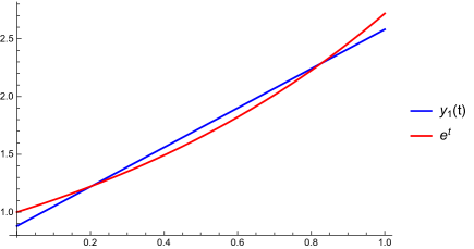
Using the approximation y1(t)=YTB(t)=BT(t)Ysubscript𝑦1𝑡superscript𝑌𝑇𝐵𝑡superscript𝐵𝑇𝑡𝑌y_{1}(t)=Y^{T}B(t)=B^{T}(t)Y, we get y1(t)=4e10+(186e)tsubscript𝑦1𝑡4𝑒10186𝑒𝑡y_{1}(t)=4e-10+(18-6e)t. In Figure 1, we compare this approximate solution y1(t)subscript𝑦1𝑡y_{1}(t) with the exact solution etsuperscript𝑒𝑡e^{t}. The absolute errors at various values of t𝑡t are shown in Table 1.

Refer to caption
Figure 1. Comparison of approximate and exact solutions of System (25) for the case r=2𝑟2r=2 and q=1𝑞1q=1.
t𝑡t Error t𝑡t Error
0.0 0.120825 0.5 0.08146
0.1 0.05579 0.6 0.07827
0.2 0.00182 0.7 0.05683
0.3 0.03992 0.8 0.01525
0.4 0.06816 0.9 0.04861
Table 1. Absolute errors in solution of System (25) with r=2𝑟2r=2 and q=1𝑞1q=1.

This is degree 1 approximation, therefore μ=1𝜇1\mu=1. Further, M=max[0,1]y(t)=e𝑀subscript01superscript𝑦𝑡𝑒M=\max_{[0,1]}y^{\prime}(t)=e. The error estimate by using (21) is M/240.169893approximately-equals-or-equals𝑀superscript240.169893M/2^{4}\approxeq 0.169893. It can be checked from Table 1 that our computed values are less than this error-bound.

Case 2: Now, we consider r=3𝑟3r=3 and q=4𝑞4q=4. A 12×12121212\times 12 matrix K𝐾K is given by:

K𝐾\displaystyle K =\displaystyle= (1.00520.12550.00520.78290.09780.00410.12550.01570.00070.09780.01220.00050.00520.00070.00.004010.00050.01.29070.16120.00671.00520.12550.00520.16120.02020.00080.12550.01570.00070.00670.00080.00.00520.00070.01.65730.20700.00861.29070.16120.00670.20700.02580.00110.16120.02010.00080.00860.00110.00.00670.00080.02.12810.26580.01111.65730.20700.00860.26570.03320.00140.20700.02580.00110.01110.00140.00.00860.00110.0\displaystyle\left(\begin{matrix}1.0052&-0.1255&0.0052&0.7829&-0.0978&0.0041\\ 0.1255&-0.0157&0.0007&0.0978&-0.0122&0.0005\\ 0.0052&-0.0007&0.0&0.00401&-0.0005&0.0\\ 1.2907&-0.1612&0.0067&1.0052&-0.1255&0.0052\\ 0.1612&-0.0202&0.0008&0.1255&-0.0157&0.0007\\ 0.0067&-0.0008&0.0&0.0052&-0.0007&0.0\\ 1.6573&-0.2070&0.0086&1.2907&-0.1612&0.0067\\ 0.2070&-0.0258&0.0011&0.1612&-0.0201&0.0008\\ 0.0086&-0.0011&0.0&0.0067&-0.0008&0.0\\ 2.1281&-0.2658&0.0111&1.6573&-0.2070&0.0086\\ 0.2657&-0.0332&0.0014&0.2070&-0.0258&0.0011\\ 0.0111&-0.0014&0.0&0.0086&-0.0011&0.0\end{matrix}\right.
0.60970.07610.00320.47480.05930.00250.07610.00950.00030.05930.00740.00030.00320.00040.00.00250.00030.00.78290.09780.00400.60970.07610.00320.09780.01220.00050.07610.00950.00040.00410.00050.00.00320.00040.01.00520.12550.00520.78290.09780.004010.12550.01570.00070.09780.01220.00050.00520.00070.00.00410.00050.01.29070.16120.00671.00520.12550.00520.16120.02010.00080.12550.01570.00070.00670.00080.00.00520.00070.0)\displaystyle\left.\begin{matrix}0.6097&-0.0761&0.0032&0.4748&-0.0593&0.0025\\ 0.0761&-0.0095&0.0003&0.0593&-0.0074&0.0003\\ 0.0032&-0.0004&0.0&0.0025&-0.0003&0.0\\ 0.7829&-0.0978&0.0040&0.6097&-0.0761&0.0032\\ 0.0978&-0.0122&0.0005&0.0761&-0.0095&0.0004\\ 0.0041&-0.0005&0.0&0.0032&-0.0004&0.0\\ 1.0052&-0.1255&0.0052&0.7829&-0.0978&0.00401\\ 0.1255&-0.0157&0.0007&0.0978&-0.0122&0.0005\\ 0.0052&-0.0007&0.0&0.0041&-0.0005&0.0\\ 1.2907&-0.1612&0.0067&1.0052&-0.1255&0.0052\\ 0.1612&-0.0201&0.0008&0.1255&-0.0157&0.0007\\ 0.0067&-0.0008&0.0&0.0052&-0.0007&0.0\end{matrix}\right)

Other approximations in this case are as below:

B(t)𝐵𝑡\displaystyle B(t) =\displaystyle= (χ[0,1/4),(1+8t)χ[0,1/4),(124t+96t2)χ[0,1/4),χ[1/4,1/2),\displaystyle\left(\chi_{[0,1/4)},(-1+8t)\chi_{[0,1/4)},(1-24t+96t^{2})\chi_{[0,1/4)},\chi_{[1/4,1/2)},\right.
(3+8t)χ[1/4,1/2),(1372t+96t2)χ[1/4,1/2),χ[1/2,3/4),(5+8t)χ[1/2,3/4),38𝑡subscript𝜒14121372𝑡96superscript𝑡2subscript𝜒1412subscript𝜒123458𝑡subscript𝜒1234\displaystyle(-3+8t)\chi_{[1/4,1/2)},(13-72t+96t^{2})\chi_{[1/4,1/2)},\chi_{[1/2,3/4)},(-5+8t)\chi_{[1/2,3/4)},
(37120t+96t2)χ[1/2,3/4),χ[3/4,1),(7+8t)χ[3/4,1),(73168t+96t2)χ[3/4,1)),\displaystyle\left.(37-120t+96t^{2})\chi_{[1/2,3/4)},\chi_{[3/4,1)},(-7+8t)\chi_{[3/4,1)},(73-168t+96t^{2})\chi_{[3/4,1)}\right),

(where χAsubscript𝜒𝐴\chi_{A} is the characteristic function of a set A𝐴A)

F𝐹\displaystyle F =\displaystyle= (3.08824,0.385629,0.0160607,3.96538,0.495157,0.0206224,\displaystyle\left(3.08824,0.385629,0.0160607,3.96538,0.495157,0.0206224,\right.
5.09165,0.635795,0.0264796,6.53781,0.816377,0.0340005)T,\displaystyle\,\,\left.5.09165,0.635795,0.0264796,6.53781,0.816377,0.0340005\right)^{T},
Y0=(1,0,0,1,0,0,1,0,0,1,0,0)T,subscript𝑌0superscript100100100100𝑇Y_{0}=\left(1,0,0,1,0,0,1,0,0,1,0,0\right)^{T},

and

Y𝑌\displaystyle Y =\displaystyle= (1.1361,0.141865,0.00590841,1.45878,0.182158,0.00758655,\displaystyle\left(1.1361,0.141865,0.00590841,1.45878,0.182158,0.00758655,\right.
1.87312,0.233896,0.00974132,2.40513,0.300328,0.0125081)T.\displaystyle\,\,\left.1.87312,0.233896,0.00974132,2.40513,0.300328,0.0125081\right)^{T}.

The approximate solution of (25) is given by

y2(t)subscript𝑦2𝑡\displaystyle y_{2}(t) =\displaystyle= 1.1361χ[0,1/4)+1.45878χ[1/4,1/2)+1.87312χ[1/2,3/4)+2.40513χ[3/4,1)1.1361subscript𝜒0141.45878subscript𝜒14121.87312subscript𝜒12342.40513subscript𝜒341\displaystyle 1.1361\chi_{[0,1/4)}+1.45878\chi_{[1/4,1/2)}+1.87312\chi_{[1/2,3/4)}+2.40513\chi_{[3/4,1)}
+0.3(7+8t)χ[3/4,1)+0.233896(5+8t)χ[1/2,3/4)0.378𝑡subscript𝜒3410.23389658𝑡subscript𝜒1234\displaystyle+0.3(-7+8t)\chi_{[3/4,1)}+0.233896(-5+8t)\chi_{[1/2,3/4)}
+0.182158(3+8t)χ[1/4,1/2)+0.14187(1+8t)χ[0,1/4)0.18215838𝑡subscript𝜒14120.1418718𝑡subscript𝜒014\displaystyle+0.182158(-3+8t)\chi_{[1/4,1/2)}+0.14187(-1+8t)\chi_{[0,1/4)}
+0.0125(73168t+96t2)χ[3/4,1)+0.0097(37120t+96t2)χ[1/2,3/4)0.012573168𝑡96superscript𝑡2subscript𝜒3410.009737120𝑡96superscript𝑡2subscript𝜒1234\displaystyle+0.0125(73-168t+96t^{2})\chi_{[3/4,1)}+0.0097(37-120t+96t^{2})\chi_{[1/2,3/4)}
+0.00759(1372t+96t2)χ[1/4,1/2)+0.00591(124t+96t2)χ[0,1/4).0.007591372𝑡96superscript𝑡2subscript𝜒14120.00591124𝑡96superscript𝑡2subscript𝜒014\displaystyle+0.00759(13-72t+96t^{2})\chi_{[1/4,1/2)}+0.00591(1-24t+96t^{2})\chi_{[0,1/4)}.

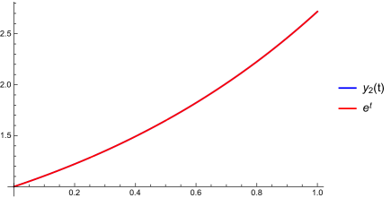
Figure 2 shows the graphs of the approximate solution y2(t)subscript𝑦2𝑡y_{2}(t) and the exact solution etsuperscript𝑒𝑡e^{t}. The absolute errors at various values of t𝑡t are given in Table 2. It can be observed that, in this case, the approximate solution is well in agreement with the exact solution. Further, using (21), the error bound is 0.014160.014160.01416. Table 2 shows that our computed maximum value is 0.0001459610.0001459610.000145961.

Refer to caption
Figure 2. Comparison of approximate and exact solutions of System (25) for the case r=3𝑟3r=3 and q=4𝑞4q=4.
t𝑡t Error t𝑡t Error
0.0 0.000145961 0.5 0.000240649
0.1 0.0000409679 0.6 0.0000675446
0.2 0.0000553281 0.7 0.0000912206
0.3 0.0000656897 0.8 0.000108304
0.4 0.0000536172 0.9 0.0000883998
Table 2. Absolute errors in solution of System (25) with r=3𝑟3r=3 and q=4𝑞4q=4.
Example 5.2.

Consider the following Volterra integro-differential system

(29) {y(t)+0tsin(ts)y(s)y(s)𝑑s=2t3+t212t+12sin(t),y(0)=0.cases𝑦𝑡superscriptsubscript0𝑡𝑡𝑠𝑦𝑠superscript𝑦𝑠differential-d𝑠2superscript𝑡3superscript𝑡212𝑡12𝑡missing-subexpression𝑦00\displaystyle\left\{\begin{array}[]{l}y(t)+\int_{0}^{t}\sin(t-s)y(s)y^{{}^{\prime}}(s)ds=2t^{3}+t^{2}-12t+12\sin(t),\\ \\ y(0)=0.\end{array}\right.

Comparing with the standard form of System (10), we get β=1,𝛽1\beta=1, g(t,s)=sin(ts)𝑔𝑡𝑠𝑡𝑠g(t,s)=\sin(t-s), m=0,𝑚0m=0, n=1𝑛1n=1, f(t)=2t3+t212t+12sin(t)𝑓𝑡2superscript𝑡3superscript𝑡212𝑡12𝑡f(t)=2t^{3}+t^{2}-12t+12\sin(t), l=0𝑙0l=0 and a0=0subscript𝑎00a_{0}=0. We take r=3𝑟3r=3 and q=4𝑞4q=4. Following the procedure described in Section 2, we get

F𝐹\displaystyle F =\displaystyle= (0.0208496,0.0312848,0.0104457,0.146854,0.0951443,0.0109877,\displaystyle\left(0.0208496,0.0312848,0.0104457,0.146854,0.0951443,0.0109877,\right.
0.406543,0.166108,0.0129514,0.824576,0.255306,0.0171862)T,\displaystyle\,\,\left.0.406543,0.166108,0.0129514,0.824576,0.255306,0.0171862\right)^{T},
G𝐺\displaystyle G =\displaystyle= (00.124500.24610.12060.00130.124500.00060.12060.00390.000600.000600.00130.000600.24610.12060.001300.124500.12060.00390.00060.124500.00060.00130.0006000.000600.47690.10920.00250.24610.12060.00130.10920.00750.00060.12060.00390.00060.00250.000600.00130.000600.67810.09110.00350.47690.10920.00250.09110.01060.00050.10920.00750.00060.00350.000500.00250.00060\displaystyle\left(\begin{matrix}0&-0.1245&0&-0.2461&-0.1206&0.0013\\ 0.1245&0&-0.0006&0.1206&-0.0039&-0.0006\\ 0&0.0006&0&0.0013&0.0006&0\\ 0.2461&-0.1206&-0.0013&0&-0.1245&0\\ 0.1206&0.0039&-0.0006&0.1245&0&-0.0006\\ -0.0013&0.0006&0&0&0.0006&0\\ 0.4769&-0.1092&-0.0025&0.2461&-0.1206&-0.0013\\ 0.1092&0.0075&-0.0006&0.1206&0.0039&-0.0006\\ -0.0025&0.0006&0&-0.0013&0.0006&0\\ 0.6781&-0.0911&-0.0035&0.4769&-0.1092&-0.0025\\ 0.0911&0.0106&-0.0005&0.1092&0.0075&-0.0006\\ -0.0035&0.0005&0&-0.0025&0.0006&0\end{matrix}\right.
0.47690.10920.00250.67810.09110.00350.10920.00750.00060.09120.01060.00050.00250.000600.00350.000500.24610.12060.00130.47690.10920.00250.12060.00390.00060.10920.00750.00060.00130.000600.00250.0006000.124500.24610.12060.00130.124500.00060.12060.00390.000600.000600.00130.000600.24610.12060.0012800.124500.12060.00390.00060.124500.00060.00130.0006000.00060),\displaystyle\left.\begin{matrix}-0.4769&-0.1092&0.0025&-0.6781&-0.0911&0.0035\\ 0.1092&-0.0075&-0.0006&0.0912&-0.0106&-0.0005\\ 0.0025&0.0006&0&0.0035&0.0005&0\\ -0.2461&-0.1206&0.0013&-0.4769&-0.1092&0.0025\\ 0.1206&-0.0039&-0.0006&0.1092&-0.0075&-0.0006\\ 0.0013&0.0006&0&0.0025&0.0006&0\\ 0&-0.1245&0&-0.2461&-0.1206&0.0013\\ 0.1245&0&-0.0006&0.1206&-0.0039&-0.0006\\ 0&0.0006&0&0.0013&0.0006&0\\ 0.2461&-0.1206&-0.00128&0&-0.1245&0\\ 0.1206&0.0039&-0.0006&0.1245&0&-0.0006\\ -0.0013&0.0006&0&0&0.0006&0\end{matrix}\right),
Y0=(0,0,0,0,0,0,0,0,0,0,0,0)T,subscript𝑌0superscript000000000000𝑇Y_{0}=\left(0,0,0,0,0,0,0,0,0,0,0,0\right)^{T},

and B(t)𝐵𝑡B(t) is same as given in the previous example. Using Equation (18), we get

Y𝑌\displaystyle Y =\displaystyle= (0.0208333,0.0312487,0.0104375,0.145833,0.0937492,0.0104781,\displaystyle\left(0.0208333,0.0312487,0.0104375,0.145833,0.0937492,0.0104781,\right.
0.395833,0.15625,0.0105145,0.770834,0.218753,0.010543)T.\displaystyle\,\,\left.0.395833,0.15625,0.0105145,0.770834,0.218753,0.010543\right)^{T}.

The approximate solution of System (29) is given by

y2(t)subscript𝑦2𝑡\displaystyle y_{2}(t) =\displaystyle= 0.0208333χ[0,1/4)+0.145833χ[1/4,1/2)0.0208333subscript𝜒0140.145833subscript𝜒1412\displaystyle 0.0208333\chi_{[0,1/4)}+0.145833\chi_{[1/4,1/2)}
+0.395833χ[1/2,3/4)+0.770834χ[3/4,1)0.395833subscript𝜒12340.770834subscript𝜒341\displaystyle+0.395833\chi_{[1/2,3/4)}+0.770834\chi_{[3/4,1)}
+0.218753(7+8t)χ[3/4,1)+0.15625(5+8t)χ[1/2,3/4)0.21875378𝑡subscript𝜒3410.1562558𝑡subscript𝜒1234\displaystyle+0.218753(-7+8t)\chi_{[3/4,1)}+0.15625(-5+8t)\chi_{[1/2,3/4)}
+0.0937492(3+8t)χ[1/4,1/2)+0.0312487(1+8t)χ[0,1/4)0.093749238𝑡subscript𝜒14120.031248718𝑡subscript𝜒014\displaystyle+0.0937492(-3+8t)\chi_{[1/4,1/2)}+0.0312487(-1+8t)\chi_{[0,1/4)}
+0.010543(73168t+96t2)χ[3/4,1)+0.0105145(37120t+96t2)χ[1/2,3/4)0.01054373168𝑡96superscript𝑡2subscript𝜒3410.010514537120𝑡96superscript𝑡2subscript𝜒1234\displaystyle+0.010543(73-168t+96t^{2})\chi_{[3/4,1)}+0.0105145(37-120t+96t^{2})\chi_{[1/2,3/4)}
+0.0104781(1372t+96t2)χ[1/4,1/2)+0.0104375(124t+96t2)χ[0,1/4).0.01047811372𝑡96superscript𝑡2subscript𝜒14120.0104375124𝑡96superscript𝑡2subscript𝜒014\displaystyle+0.0104781(13-72t+96t^{2})\chi_{[1/4,1/2)}+0.0104375(1-24t+96t^{2})\chi_{[0,1/4)}.

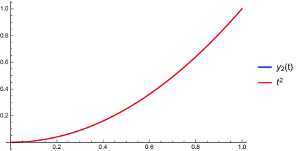
The approximate solution y2(t)subscript𝑦2𝑡y_{2}(t) is compared with the exact solution t2superscript𝑡2t^{2} in Figure 3. Table 3 shows the absolute error in the solution at different values of t𝑡t.

Refer to caption
Figure 3. Comparison of approximate and exact solutions of System (29) for the case r=3𝑟3r=3 and q=4𝑞4q=4.
t𝑡t Error t𝑡t Error
0.0 0.0000221689 0.5 0.0000975226
0.1 8.9×10⁶absentsuperscript106\times 10^{-6} 0.6 0.0000429716
0.2 4.99×10⁸absentsuperscript108\times 10^{-8} 0.7 4.32×10⁶absentsuperscript106\times 10^{-6}
0.3 3×10⁶absentsuperscript106\times 10^{-6} 0.8 3.76×10⁶absentsuperscript106\times 10^{-6}
0.4 0.0000271471 0.9 0.0000547743
Table 3. Absolute errors in solution of System (29) with r=3𝑟3r=3 and q=4𝑞4q=4.

Using (21), the error-bound for this example is approximately 0.01041670.01041670.0104167 and our value from Table 3 is 0.00002714710.00002714710.0000271471.

6. Conclusion

In this work, we have discussed an efficient method to solve a class of Fredholm and Volterra integro-differential equations. Our method is based on a new approximation for the derivatives of the equations’ solutions using hybrid and block-pulse functions. The absolute errors reported in tables show that the approximate solution is in a good agreement with the exact solution. It is verified in each example that the practical error in our method is less than the theoretical error-bound. In fact, this method is highly efficient, very easy and a powerful mathematical tool for finding the numerical solution of some class of Fredholm and Volterra integro-differential equations. The approximate solutions are found by using the computer code written in Matlab. The method is computationally attractive, and applications are demonstrated through illustrative examples. For future research works, we can use this method to solve various kinds of problems such as higher dimensional problems, stochastic integro-differential equations and partial integro-differential equations of fractional order with additional work.

References

  • [1] S. Abbasbandy and E. Shivanian, Application of variational iteration method for nth-order integro-differential equations, Zeitschrift fur Naturforschung A, 64 (6-7) (2009), 439-444.
  • [2] M.A. Abdou, On asymptotic methods for Fredholm-Volterra integral equation of the second kind in contact problems, J. Comput. Appl. Math., 154 (2003), 431-446.
  • [3] B. Basirat, K. Maleknejad and E. Hashemizadeh, Operational matrix approach for the nonlinear Volterra-Fredholm integral equations: Arising in physics and engineering, International Journal of Physical Sciences, 7.2 (2012), 226-233 .
  • [4] F. Bloom, Asymptotic bounds for solutions to a system of damped integro-differential equations of electromagnetic theory, J. Math. Anal. Appl., 73 (1980), 524-542.
  • [5] V. Daftardar-Gejji and H. Jafari, An iterative method for solving non-linear functional equations, J. Math. Anal. Appl., 316 (2006), 753-763.
  • [6] L.M. Delves and J.L. Mohamed, Computational methods for integral equations, Cambridge University Press, Cambridge (1985).
  • [7] L.K. Forbes, S. Crozier and D.M. Doddrell, Calculating current densities and fields produced by shielded magnetic resonance imaging probes, SIAM J. Appl. Math., 57 (2) (1997), 401-425.
  • [8] J. Frankel, A Galerkin solution to regularized Cauchy singular integro-differential equation, Quart. Appl. Math., 52 (2) (1995), 145-258.
  • [9] A. Golbabai and M. Javidi, Application of He’s homotopy perturbation method for nthsuperscript𝑛𝑡n^{th}-order integro-differential equations, Appl. Math. Comput., 190 (2007), 1409-1416.
  • [10] M.A. Golberg, The convergence of a collocations method for a class of Cauchy singular integral equations, J. Math. Appl., 100 (1984), 500-512.
  • [11] E. Hashemizadeh and B. Basirat, An efficient computational method for the system of linear Volterra integral equations by means of hybrid functions, Mathematical Sciences, 5 (4) (2011), 355-368.
  • [12] A. A. Hemeda, New iterative method: application to nthsuperscript𝑛𝑡n^{th}-order integro-differential equations, International Mathematical Forum, Vol. 7 (47) (2012), 2317-2332.
  • [13] J. Hou and C. Yang, Numerical method in solving Fredholm integro-differential equations by using hybrid function operational matrix of derivative, Journal of Information and Computational Science, 10:9 (2013), 2757-2764.
  • [14] K. Holmaker, Global asymptotic stability for a stationary solution of a system of integro-differential equations describing the formation of liver zones, SIAM J. Math. Anal., 24 (1) (1993), 116-128.
  • [15] C.H. Hsiao, Hybrid function method for solving Fredholm and Volterra integral equations of the second kind, J. Comput. Appl. Math., 230 (2009), 59-68.
  • [16] E.V. Kovalenko, Some approximate methods for solving integral equations of mixed problems, Provl. Math. Mech., 53 (1) (1989), 85-92.
  • [17] K. Maleknejad, B. Basirat and E. Hashemizadeh, Hybrid Legendre polynomials and block-pulse functions approach for nonlinear Volterra-Fredholm integro-differential equations, Comput. Math. Appl., 61(9) (2011), 282-288.
  • [18] H.R. Marzban and M. Razzaghi, Optimal control of linear delay systems via hybrid of block-pulse and Legendre polynomials, J. Franklin Inst., 341(3) (2004), 279-293.
  • [19] F. Mizaee, Numerical solution of system of linear integral equations via improvement of block-pulse functions, Journal of Mathematical Modeling, 4 (2) (2016), 133-159.
  • [20] F. Mizaee, S. Alipour, Approximate solution of nonlinear quadratic integral equations of fractional order via piecewise linear functions, Journal of Computational and Applied Mathematics, 331 (2018) 217-227.
  • [21] F. Mizaee, S. Alipour and N. Samadyar, Numerical solution based on hybrid of block-pulse and parabolic functions for solving a system of nonlinear stochastic Ito-Volterra integral equations of fractional order, Journal of Computational and Applied Mathematics, 349 (2019),157-171.
  • [22] F. Mizaee and S. F. Hoseini, A new collocation approach for solving systems of high-order linear Volterra integro-differential equations with variable coefficients, Applied Mathematics and Computation, 311 (2017) 72-282.
  • [23] F. Mizaee and S. F. Hoseini, Hybrid functions of Bernstein polynomials and block-pulse functions for solving optimal control of the nonlinear Volterra integral equations, Indagationes Mathematicae, 27 (3) (2016), 835-849.
  • [24] A.D. Polyanin and A.V. Manzhirov, Handbook of integral equations (2nd ed.), Chapman and Hall/CRC Press, Boca Raton- London (2008).
  • [25] M. Razzaghi and H.R. Marzban, A hybrid analysis direct method in the calculus of variations, Int. J. Comput. Math., 75 (2000), 259-269.
  • [26] B.J. Semetanian, On an integral equation for axially symmetric problem in the case of an elastic body containing an inclusion, J. Appl. Math. Mech., 55 (3) (1991), 371-375.
  • [27] X. Shang and D. Han, Application of the variational iteration method for solving nthsuperscript𝑛𝑡n^{th}-order integro-differential equations, Journal of Computational and Applied Mathematics, 234 (5) (2010), 1442-1447.
  • [28] T. Shojaeizadeh, Z. Abadi, and E. Golpar Raboky, Hybrid functions approach for solving Fredholm and Volterra integral equations, J. Prime Res. Math., 5 (2009), 124-132.
  • [29] G. W. Stewart, Afternotes on numerical analysis, Vol. 49. SIAM, 1996.
  • [30] A.M. Wazwaz, A first course in integral equations, World Scientifics, Singapore (1997).
  • [31] J.R. Willis and S. Nemat-Nasser, Singular perturbation solution of a class of singular integral equations, Quart. Appl. Math., XLVIII (4) (1990), 741-753.