Stable Phaseless Sampling and Reconstruction of Real-Valued Signals with Finite Rate of Innovations

Abstract.

A spatial signal is defined by its evaluations on the whole domain. In this paper, we consider stable reconstruction of real-valued signals with finite rate of innovations (FRI), up to a sign, from their magnitude measurements on the whole domain or their phaseless samples on a discrete subset. FRI signals appear in many engineering applications such as magnetic resonance spectrum, ultra wide-band communication and electrocardiogram. For an FRI signal, we introduce an undirected graph to describe its topological structure. We establish the equivalence between the graph connectivity and phase retrievability of FRI signals, and we apply the graph connected component decomposition to find all FRI signals that have the same magnitude measurements as the original FRI signal has. We construct discrete sets with finite density explicitly so that magnitude measurements of FRI signals on the whole domain are determined by their samples taken on those discrete subsets. In this paper, we also propose a stable algorithm with linear complexity to reconstruct FRI signals from their phaseless samples on the above phaseless sampling set. The proposed algorithm is demonstrated theoretically and numerically to provide a suboptimal approximation to the original FRI signal in magnitude measurements.

1. Introduction

A spatial signal $f$ on a domain $D$ is defined by its evaluations $f(x),x\in D$. In this paper, we consider the problem whether and how a real-valued signal $f$ can be reconstructed, up to a global sign, from magnitude information $|f(x)|,x\in D$, or from its phaseless samples $|f(\gamma)|,\gamma\in\Gamma$, taken on a discrete set $\Gamma\subset D$ in a stable way. The above problem has been discussed for bandlimited signals [39] and wavelet signals residing in a principal shift-invariant space [13, 14, 38]. It is a nonlinear ill-posed problem which can be solved only if we have some extra information about the signal $f$. In this paper, we always assume that the signal $f$ has a parametric representation,

(1.1) $$f(x)=\sum_{\lambda\in\Lambda}c_{\lambda}\phi_{\lambda}(x),\ x\in D,$$

where $c=(c_{\lambda})_{\lambda\in\Lambda}$ is an unknown real-valued parameter vector, $\Lambda\subset D$ is a discrete set with finite density, and $\Phi=(\phi_{\lambda})_{\lambda\in\Lambda}$ is a vector of nonzero basis signals $\phi_{\lambda},\lambda\in\Lambda$, essentially supported in a neighborhood of the innovative position $\lambda\in\Lambda$. Those signals appear in many engineering applications such as magnetic resonance spectrum, ultra wide-band communication and electrocardiogram. Our representing signals of the form (1.1) are bandlimited signals, signals in a shift-invariant space and spline signals on triangulations. Following the terminology in [41], signals of the form (1.1) have finite rate of innovations (FRI) and their rate of innovations is the density of the set $\Lambda$ [16, 17, 35, 41].

Given a signal $f$ with the parametric representation (1.1), let ${\mathcal{M}}_{f}$ contain all signals $g$ of the form (1.1) such that

(1.2) $$|g(x)|=|f(x)|,\ x\in D.$$

As $-f$ and $f$ have the same magnitude measurements on the whole domain, we have that ${\mathcal{M}}_{f}\supset\{\pm f\}$. A natural question is whether the above inclusion is an equality.

Question 1.1.

Can we characterize all signals $f$ of the form (1.1) so that ${\mathcal{M}}_{f}=\{\pm f\}$?

An equivalent statement to the above question is whether a signal $f$ is determined, up to a sign, from the magnitude information $|f(x)|,x\in D$. The above question is an infinite-dimensional phase retrieval problem, which has been discussed for bandlimited signals [39], wavelet signals in a principal shift-invariant space [13, 14, 38], and spatial signals in a linear space [13]. The reader may refer to [1, 2, 8, 20, 27, 28, 33] for historical remarks and additional references on phase retrieval in an infinite-dimensional linear space. In Section 3, we introduce an undirected graph ${\mathcal{G}}_{f}$ for a signal $f$ of the form (1.1), and we provide an answer to Question 1.1 by showing that ${\mathcal{M}}_{f}=\{\pm f\}$ if and only if ${\mathcal{G}}_{f}$ is connected, see Theorem 3.2.

For a signal $f$ with a parametric representation (1.1), the graph ${\mathcal{G}}_{f}$ is not necessarily to be connected. This leads to our next question.

Question 1.2.

Can we find the set ${\mathcal{M}}_{f}$ for any signal $f$ of the form (1.1)?

For a signal $f$ of the form (1.1), we can decompose its graph ${\mathcal{G}}_{f}$ uniquely to a union of connected components ${\mathcal{G}}_{i},i\in I$,

(1.3) $${\mathcal{G}}_{f}=\cup_{i\in I}{\mathcal{G}}_{i}.$$

Then we can construct signals $f_{i},i\in I$, of the form (1.1) with ${\mathcal{G}}_{f_{i}}={\mathcal{G}}_{i},i\in I$, such that

(1.4) $$f_{i}f_{i^{\prime}}=0\ {\rm for\ all\ distinct}\ i,i^{\prime}\in I,$$

(1.5) $${\mathcal{M}}_{f_{i}}=\{\pm f_{i}\},\ i\in I,$$

and

(1.6) $$f=\sum_{i\in I}f_{i},$$

see Theorem 4.3. Due to the mutually disjoint support property (1.4) for signals $f_{i},i\in I$, and the connectivity for the graphs ${\mathcal{G}}_{f_{i}},i\in I$, we can interprete the above adaptive decomposition as that landscape of the original signal $f$ is composed by islands of signals $f_{i},i\in I$, see Figure 1 and also [1, 20] for bandlimited signals.

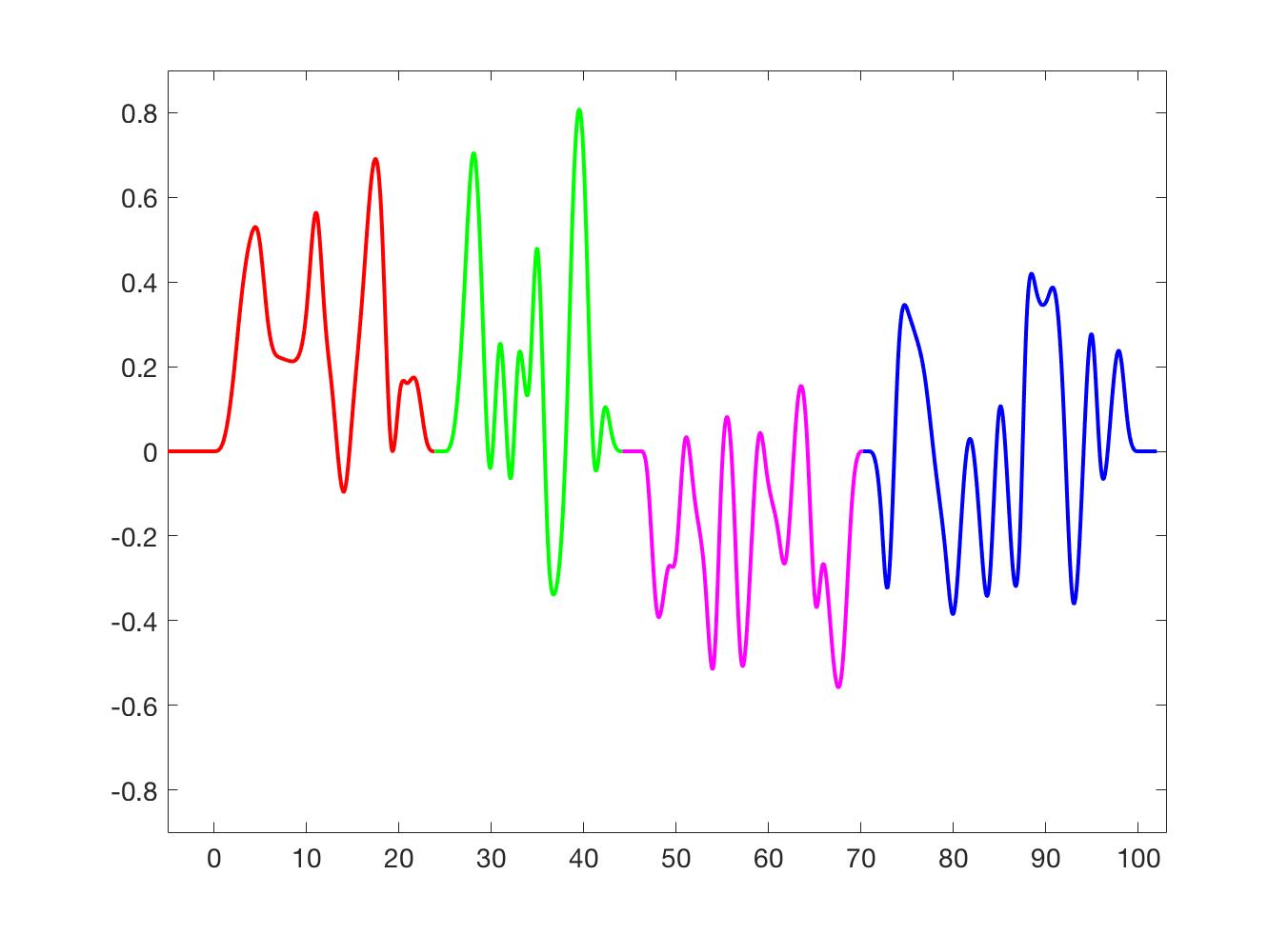
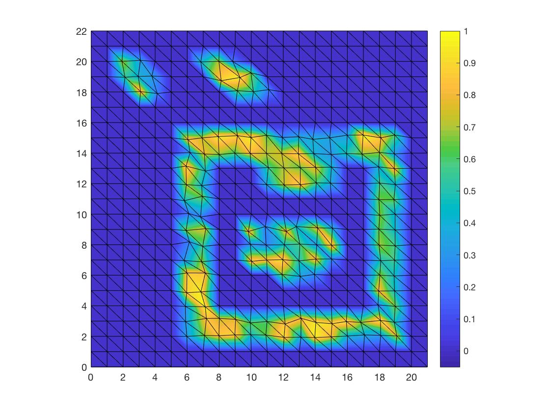
Figure 1. Plotted on the left is a non-uniform cubic spline signal, while on the right is a piecewise affine signal on a triangulation. They both have four “islands” in the decomposition (1.4), (1.5) and (1.6).

By (1.4) and (1.6), we have

$${\mathcal{M}}_{f}\supset\Big{\{}\sum_{i\in I}\delta_{i}f_{i},\ \delta_{i}\in\{-1,1\},i\in I\Big{\}}.$$

In Section 4, we provide an answer to Question 1.2 by showing in Theorem 4.1 that the above inclusion is in fact an equality for any signal $f$ of the form (1.1). Therefore landscapes of signals $g\in{\mathcal{M}}_{f}$ are combination of islands of the original signal $f$ and their reflections.

Let $f$ be a signal of the form (1.1). To consider phaseless sampling and reconstruction on a discrete set $\Gamma\subset D$, we let ${\mathcal{M}}_{f,\Gamma}$ contain all signals $g$ of the form (1.1) such that

(1.7) $$|g(\gamma)|=|f(\gamma)|,\ \gamma\in\Gamma,$$

and ${\mathcal{N}}_{\Gamma}$ contain all signals $h$ of the form (1.1) such that

(1.8) $$h(\gamma)=0,\ \gamma\in\Gamma.$$

By (1.2), (1.7) and (1.8), we have

(1.9) $${\mathcal{M}}_{f}={\mathcal{M}}_{f,D},\ {\mathcal{N}}_{D}=\{0\},$$

and

(1.10) $${\mathcal{M}}_{f}+{\mathcal{N}}_{\Gamma}\subset{\mathcal{M}}_{f,\Gamma}\ {\rm for\ all}\ \Gamma\subset D.$$

This leads to the third question.

Question 1.3.

Can we find all discrete sets $\Gamma$ such that ${\mathcal{M}}_{f,\Gamma}={\mathcal{M}}_{f}$ for all signals $f$ of the form (1.1)?

By (1.10), a necessary condition for the equality ${\mathcal{M}}_{f,\Gamma}={\mathcal{M}}_{f}$ to hold for some signal $f$ of the form (1.1) is that ${\mathcal{N}}_{\Gamma}=\{0\}$, which means that all signals of the form (1.1) are determined from their samples taken on $\Gamma$. The reader may refer to [17, 34, 37, 41] and references therein for stable sampling and reconstruction of FRI signals.

In Section 5, we show the existence of a discrete set $\Gamma$ with finite density such that ${\mathcal{M}}_{f,\Gamma}={\mathcal{M}}_{f}$ for all signals $f$ of the form (1.1). In Theorem 5.2, we construct such a discrete set $\Gamma$ explicitly under the assumption that the linear space for signals of the form (1.1) to reside in has local complement property on a family of open sets. The local complement property, see Definition 3.1, is introduced in [14] and it is closely related to the complement property for ideal sampling functionals in [13] and the complement property for frames in Hilbert/Banach spaces [2, 4, 6, 8]. The local complement property on a bounded open set can be characterized by phase retrievable frames associated with the generator $\Phi$ and the sampling set $\Gamma$ on a finite-dimensional space, see Proposition 5.4. The reader may refer to [3, 4, 9, 10, 11, 18, 21, 23, 31, 43] and references therein for historical remarks and recent advances on finite-dimensional phase retrievable frames.

An equivalent statement to the equality ${\mathcal{M}}_{f,\Gamma}={\mathcal{M}}_{f}$ is that magnitude measurements $|f(x)|,x\in D$, on the whole domain $D$ are determined by their samples $|f(\gamma)|,\gamma\in\Gamma$, taken on a discrete set $\Gamma$. In practical applications, phaseless samples are usually corrupted by some bounded deterministic/random noises $\eta(\gamma),\gamma\in\Gamma$, and the available noisy phaseless samples are

$$z_{\eta}(\gamma)=|f(\gamma)|+\eta(\gamma),\ \gamma\in\Gamma.$$

Set $\eta=(\eta(\gamma))_{\gamma\in\Gamma}$ and $z_{\eta}=(z_{\eta}(\gamma))_{\gamma\in\Gamma}$. This leads to the fourth question to be discussed in this paper.

Question 1.4.

Can we find an algorithm $\Delta$ such that the reconstructed signal $g_{\eta}=\Delta(z_{\eta})$ is an approximation to the original signal $f$ in magnitude measurements?

In Section 6, we propose an algorithm with linear complexity, which provides an answer to Question 1.4. Under the assumption that the generator $\Phi$ is well localized and uniformly bounded, we show in Theorem 6.2 that the original signal $f$ and the reconstructed signal $g_{\eta}$ are well approximated by some signals $f_{\eta}$ and $h_{\eta}$ of the form (1.1) that have the same magnitude measurements on the domain $D$. Therefore the reconstructed signal $g_{\eta}$ provides a suboptimal approximation to the original signal $f$ in magnitude measurements, i.e., there exists an absolute constant $C$ independent on the original signal $f$ and the noise $\eta$ such that

(1.11) $$\sup_{x\in D}\big{|}|g_{\eta}(x)|-|f(x)|\big{|}\leq C\sup_{\gamma\in\Gamma}|\eta(\gamma)|.$$

As an application of the above estimate, we conclude that the phaseless sampling operator $S:f\longmapsto(|f(\gamma)|)_{\gamma\in\Gamma}$ is bi-Lipschitz in magnitude measurements, see Corollary 6.3.

The paper is organized as follows. In Section 2, we present some preliminaries on the linear space $V(\Phi)$ for signals of the form (1.1) to reside in. In Section 3, we introduce a graph structure for any signal in $V(\Phi)$ and use its connectivity to provide an answer to Question 1.1. In Section 4, we introduce a landscape decomposition for a signal $f\in V(\Phi)$ and use it to find all signals in ${\mathcal{M}}_{f}$. In Section 5, we construct a discrete set $\Gamma$ with finite density such that ${\mathcal{M}}_{f,\Gamma}={\mathcal{M}}_{f}$ for all $f\in V(\Phi)$. In Section 6, we introduce a stable algorithm $\Delta$ with linear complexity to reconstruct signals in $V(\Phi)$ from their noisy phaseless samples taken on a discrete set $\Gamma$. In Section 7, we demonstrate the stable reconstruction of our proposed algorithm $\Delta$ to reconstruct one-dimensional non-uniform spline signals and two-dimensional piecewise affine signals on triangulations from their noisy phaseless samples. In Appendix A, we show that the density of a discrete set $\Gamma$ with ${\mathcal{M}}_{f,\Gamma}={\mathcal{M}}_{f},f\in V(\Phi)$, must be no less than the innovation rate of signals in $V(\Phi)$.

2. Preliminaries

In this section, we present some preliminaries on the domain $D$ for signals to define and the linear space $V(\Phi)$ for signals with the parametric expression (1.1) to reside in.

Spatial signals in this paper are defined on a domain $D$. Our representing models are the $d$-dimensional Euclidean space ${{\mathbb{R}}}^{d}$, the $d$-dimensional torus ${\mathbb{T}}^{d}$ and the simple graph to describe a spatially distributed network [15]. In this paper, we always assume the following for the domain $D$ [15, 26, 44].

Assumption 2.1.

The domain $D$ is equipped with a distance $\rho$ and a Borel measure $\mu$ so that

(2.1) $$\sup_{x\in D}\mu\big{(}B(x,r)\big{)}<\infty$$

and

(2.2) $$\liminf_{s\to\infty}\inf_{x\in D}\frac{\mu(B(x,s-r))}{\mu(B(x,s))}=1,\ r\geq 0,$$

where $B(x,r)=\{y\in D:\ \rho(x,y)\leq r\}$ is the closed ball with center $x$ and radius $r$.

Spatial signals $f$ with the parametric representation (1.1) reside in the linear space

(2.3) $$V(\Phi):=\Big{\{}\sum_{\lambda\in\Lambda}c_{\lambda}\phi_{\lambda}:\ c_{\lambda}\in{\mathbb{R}}\ {\rm for\ all}\ \lambda\in\Lambda\Big{\}}$$

generated by $\Phi=(\phi_{\lambda})_{\lambda\in\Lambda}$. Denote the cardinality of a set $E$ by $\#E$. In this paper, we always assume the following to basis signals $\phi_{\lambda},\lambda\in\Lambda$.

Assumption 2.2.

The discrete set $\Lambda$ has finite density

(2.4) $$D_{+}(\Lambda):=\limsup\limits_{{r\to\infty}}\ \sup_{x\in D}\frac{\sharp\big{(}\Lambda\cap B(x,r)\big{)}}{\mu\big{(}B(x,r)\big{)}}<\infty,$$

the nonzero basis signals $\phi_{\lambda},\lambda\in\Lambda$, are continuous and supported in balls with center $\lambda$ and fixed radius $r_{0}>0$ independent of $\lambda$,

(2.5) $$\phi_{\lambda}(x)=0\ {\rm for\ all}\ x\not\in B(\lambda,r_{0}),\ \lambda\in\Lambda;$$

and any signal in $V(\Phi)$ has a unique parametric representation (1.1).

The prototypical forms of the space $V(\Phi)$ are principal shift-invariant spaces generated by the shifts of a compactly supported function $\phi$, twisted shift-invariant spaces generated by (non-)uniform Gabor frame system (or Wilson basis) in the time-frequency analysis (see [5, 12, 19, 24, 30] and references therein), and nonuniform spline signals [7, 22, 32]. The linear space $V(\Phi)$ was introduced in [36, 37] to model signals with finite rate of innovation (FRI). Following the terminology in [41], signals in the linear space $V(\Phi)$ have rate of innovation $D_{+}(\Lambda)$ and innovative positions $\lambda\in\Lambda$.

An equivalent statement to the unique parametric representation (1.1) of signals in $V(\Phi)$ is that the generator $\Phi$ has global linear independence, i.e., the map

(2.6) $$c:=(c_{\lambda})_{\lambda\in\Lambda}\longmapsto c^{T}\Phi:=\sum_{\lambda\in\Lambda}c_{\lambda}\phi_{\lambda}$$

is one-to-one from the space $\ell(\Lambda)$ of all sequences on $\Lambda$ to the linear space $V(\Phi)$ [25, 29]. For any open set $A$, define

(2.7) $$K_{A}=\{\lambda\in\Lambda:\ \phi_{\lambda}\not\equiv 0\ {\rm on}\ A\}.$$

A strong version of the global linear independence (2.6) is local linear independence on an open set $A\subset D$, i.e.,

(2.8) $$\dim V(\Phi)|_{A}=\#K_{A},$$

where for a linear space $V$ we denote its dimension and restriction on a set $A$ by $\dim V$ and $V|_{A}$ respectively. Observe that the restriction of the linear space $V(\Phi)$ on an bounded open set $A$ is generated by $\phi_{\lambda},\lambda\in K_{A}$. Then an equivalent formulation of the local linear independence on a bounded open set $A$ is that

(2.9) $$\sum_{\lambda\in\Lambda}c_{\lambda}\phi_{\lambda}(x)=0\ {\rm on}\ x\in A$$

implies that $c_{\lambda}=0$ for all $\lambda\in K_{A}$ [25, 35].

Set

(2.10) $$S_{\Phi}(\lambda,\lambda^{\prime}):=\{x\in D:\ \phi_{\lambda}(x)\phi_{\lambda^{\prime}}(x)\neq 0\},\ \lambda,\lambda^{\prime}\in\Lambda,$$

and use the abbreviation $S_{\Phi}(\lambda):=S_{\Phi}(\lambda,\lambda)$ when $\lambda^{\prime}=\lambda\in\Lambda$. One may verify that the generator $\Phi$ has global linear independence (2.6) if it has local linear independence on a family of open sets $T_{\theta},\theta\in\Theta$, such that

(2.11) $$S_{\Phi}(\lambda,\lambda^{\prime})\cap\big{(}\cup_{\theta\in\Theta}T_{\theta}\big{)}\neq\emptyset$$

for all pairs $(\lambda,\lambda^{\prime})\in\Lambda\times\Lambda$ with $S_{\Phi}(\lambda,\lambda^{\prime})\neq\emptyset$. We remark that a family of open sets $T_{\theta},\theta\in\Theta$, satisfying (2.11) is not necessarily a covering of the domain $D$, however, the converse is true, cf. Corollary 4.4.

3. Phase retrievability and graph connectivity

In this section, we characterize all signals $f\in V(\Phi)$ that are determined, up to a sign, from their magnitude measurements on the whole domain $D$, i.e., ${\mathcal{M}}_{f}=\{\pm f\}$.

Given a signal $f=\sum_{\lambda\in\Lambda}c_{\lambda}\phi_{\lambda}\in V(\Phi)$, we define an undirected graph

(3.1) $${\mathcal{G}}_{f}:=(V_{f},E_{f}),$$

where

(3.2) $$V_{f}:=\{\lambda\in\Lambda:\ c_{\lambda}\neq 0\}$$

and

$$E_{f}:=\big{\{}({\lambda},{\lambda}^{\prime})\in V_{f}\times V_{f}:\ {\lambda}\neq{\lambda}^{\prime}\ {\rm and}\ \phi_{\lambda}\phi_{\lambda^{\prime}}\not\equiv 0\big{\}}.$$

For a signal $f\in V(\Phi)$, the graph ${\mathcal{G}}_{f}$ in (3.1) is well-defined by (2.6), and it was introduced in [14] when the generator $\Phi=(\phi(\cdot-k))_{k\in{\mathbb{Z}}^{d}}$ is obtained from shifts of a compactly supported function $\phi$. Its vertex set $V_{f}$ contains all innovative positions $\lambda\in\Lambda$ with nonzero amplitude $c_{\lambda}$, and its edge set $E_{f}$ contains all innovative position pairs $(\lambda,\lambda^{\prime})$ in $V_{f}\times V_{f}$ with basis signals $\phi_{\lambda}$ and $\phi_{\lambda^{\prime}}$ having overlapped supports, i.e.,

(3.3) $$(\lambda,\lambda^{\prime})\in E_{f}\ {\rm if\ and\ only\ if}\ \lambda,\lambda^{\prime}\in V_{f}\ {\rm and}\ (\lambda,\lambda^{\prime})\in E_{\Phi},$$

where $S_{\Phi}(\lambda,\lambda^{\prime}),(\lambda,\lambda^{\prime})\in\Lambda\times\Lambda$, are given in (2.10) and

(3.4) $$E_{\Phi}:=\{(\lambda,\lambda^{\prime})\in\Lambda\times\Lambda:\ S_{\Phi}(\lambda,\lambda^{\prime})\neq\emptyset\}.$$

To study phase retrievability of signals in $V(\Phi)$, we recall the local complement property of a linear space of real-valued signals [14].

Definition 3.1.

Let $A$ be an open subset of the domain $D$. We say that a linear space $V$ of real-valued signals on the domain $D$ has local complement property on $A$ if for any $A^{\prime}\subset A$, there does not exist $f,g\in V$ such that $f,g\not\equiv 0$ on $A$, but $f({x})=0$ for all ${x}\in A^{\prime}$ and $g({y})=0$ for all ${y}\in A\backslash A^{\prime}$.

The local complement property is the complement property in [13] for ideal sampling functionals on a set, cf. the complement property for frames in Hilbert/Banach spaces ([2, 4, 6, 8]). Local complement property is closely related to local phase retrievability. In fact, following the argument in [13], the linear space $V$ has the local complement property on $A$ if and only if all signals in $V$ is local phase retrievable on $A$, i.e., for any $f,g\in V$ satisfying $|g({x})|=|f({x})|,{x}\in A$, there exists $\delta\in\{-1,1\}$ such that $g({x})=\delta f({x})$ for all ${x}\in A$.

In this section, we establish the equivalence between phase retrievability of a nonzero signal $f\in V(\Phi)$ and connectivity of its graph ${\mathcal{G}}_{f}$, which is established in [14] for signals residing in a principal shift-invariant space.

Theorem 3.2.

Let $D$ be a domain satisfying Assumption 2.1, $\Phi:=(\phi_{\lambda})_{\lambda\in\Lambda}$ be a family of basis functions satisfying Assumption 2.2, ${\mathcal{T}}:=\{T_{\theta},\theta\in\Theta\}$ be a family of open sets satisfying (2.11), and let $V(\Phi)$ be the linear space (2.3) generated by $\Phi$. Assume that for any $T_{\theta}\in\mathcal{T}$, $\Phi$ has local linear independence on $T_{\theta}$ and $V(\Phi)$ has local complement property on $T_{\theta}$. Then for a nonzero signal $f\in V(\Phi)$, ${\mathcal{M}}_{f}=\{\pm f\}$ if and only if the graph ${\mathcal{G}}_{f}$ in (3.1) is connected.

We remark that the local complement assumption in Theorem 3.2 is satisfied when $\Phi$ has local linear independence on all open sets.

Proposition 3.3.

Let $\Phi:=(\phi_{\lambda})_{\lambda\in\Lambda}$ satisfy Assumption 2.2. If $\Phi$ has local linear independence on all open sets, then there exist ${\mathcal{T}}:=\{T_{\theta},\theta\in\Theta\}$ satisfying (2.11) such that $V(\Phi)$ has local complement property on every $T_{\theta}\in{\mathcal{T}}$.

Proof.

Define $S_{\Phi}(\theta)=\cap_{\lambda\in\theta}S_{\Phi}(\lambda)$ for a set $\theta\subset\Lambda$. We say that $\theta\subset\Lambda$ is maximal if $S_{\Phi}(\theta)\neq\emptyset$ and $S_{\Phi}(\theta^{\prime})=\emptyset$ for all $\theta^{\prime}\supsetneq\theta$. By (2.4) and (2.5), any maximal set contains finitely many elements. Denote the family of all maximal sets by $\Theta$ and define $T_{\theta}=S_{\Phi}(\theta),\theta\in\Theta$. Clearly ${\mathcal{T}}:=\{T_{\theta},\theta\in\Theta\}$ satisfies (2.11), because any $\theta\subset\Lambda$ with $S_{\Phi}(\theta)\neq\emptyset$ is a subset of some maximal set in $\Theta$.

Now it remains to prove that $V(\Phi)$ has local complement property on $T_{\theta},\theta\in\Theta$. Take an arbitrary $\theta\in\Theta$ and two signals $f,g\in V(\Phi)$ satisfying $|f(x)|=|g(x)|$ for all $x\in T_{\theta}$. Then

(3.5) $$(f+g)(x)(f-g)(x)=0\ {\rm for\ all}\ x\in T_{\theta}.$$

Write $f+g=\sum_{\lambda\in\Lambda}c_{\lambda}\phi_{\lambda}$ and $f-g=\sum_{\lambda\in\Lambda}d_{\lambda}\phi_{\lambda}$, and set $B_{1}=\{x\in T_{\theta}:\ (f+g)(x)\neq 0\}$ and $B_{2}=\{x\in T_{\theta}:\ (f-g)(x)\neq 0\}$. Then

(3.6) $$\Big{(}\sum_{\lambda\in\theta}c_{\lambda}\phi_{\lambda}(x)\Big{)}\Big{(}\sum_{\lambda\in\theta}d_{\lambda}\phi_{\lambda}(x)\Big{)}=0\ {\rm for\ all}\ x\in T_{\theta},$$

and

(3.7) $$\ \phi_{\lambda}(x)\neq 0\ {\rm for\ all}\ x\in T_{\theta}\ {\rm and}\ \lambda\in\theta$$

by assumption (2.11), (3.5) and the construction of maximal sets. By (3.6), we have that either $f-g=0$ on $B_{1}$, or $f+g=0$ on $B_{2}$, or $f-g=f+g=0$ on $T_{\theta}$. This together with (3.7) and the local linear independence on $B_{1}$ or $B_{2}$ or $T_{\theta}$ implies that either $d_{\lambda}=0$ for all $\lambda\in\theta$, or $c_{\lambda}=0$ for all $\lambda\in\theta$, or $c_{\lambda}=d_{\lambda}=0$ for all $\lambda\in\theta$. Therefore either $f=g$ on $T_{\theta}$, or $f=-g$ on $T_{\theta}$, or $f=g=0$ on $T_{\theta}$. This completes the proof. ∎

Applying Theorem 3.2 and Proposition 3.3, we have the following corollary, which is established in [14] when the generator $\Phi$ is obtained from shifts of a compactly supported function.

Corollary 3.4.

Let $D$ be a domain satisfying Assumption 2.1, $\Phi$ be a family of basis functions satisfying Assumption 2.2, and let $V(\Phi)$ be the linear space (2.3) generated by $\Phi$. If $\Phi$ has local linear independence on any open sets, then a nonzero signal $f\in V(\Phi)$ satisfies ${\mathcal{M}}_{f}=\{\pm f\}$ if and only if the graph ${\mathcal{G}}_{f}$ in (3.1) is connected.

3.1. Proof of Theorem 3.2

The necessity in Theorem 3.2 holds under a weak assumption on the generator $\Phi$.

Proposition 3.5.

Let $D$ be a domain satisfying Assumption 2.1, $\Phi:=(\phi_{\lambda})_{\lambda\in\Lambda}$ be a family of basis functions satisfying Assumption 2.2, $V(\Phi)$ be the linear space (2.3) generated by $\Phi$, and let $f$ be a nonzero signal in $V(\Phi)$. If ${\mathcal{M}}_{f}=\{\pm f\}$, then the graph ${\mathcal{G}}_{f}$ in (3.1) is connected.

To prove Proposition 3.5, we recall a characterization in [13] on phase retrievability.

Lemma 3.6.

For a nonzero signal $f$ in a linear space $V$, ${\mathcal{M}}_{f}=\{\pm f\}$ if and only if it is nonseparable, i.e., there does not exist nonzero signals $f_{0}$ and $f_{1}\in V$ such that

(3.8) $$f=f_{0}+f_{1}\ \ {\rm and}\ \ f_{0}f_{1}=0.$$

Proof of Proposition 3.5.

Let $f\in V(\Phi)$ be a nonzero signal satisfying ${\mathcal{M}}_{f}=\{\pm f\}$, and write $f=\sum_{\lambda\in\Lambda}c_{\lambda}\phi_{\lambda}$, where $c_{\lambda}\in{\mathbb{R}},\lambda\in\Lambda$. Suppose, on the contrary, that the graph ${\mathcal{G}}_{f}$ is disconnected. Then there exists a nontrivial connected component $W$ such that both $W$ and $V_{f}\backslash W$ are nontrivial, and no edges exist between vertices in $W$ and in $V_{f}\backslash W$. Write

(3.9) $$f=\sum_{k\in V_{f}}c_{\lambda}\phi_{\lambda}=\sum_{{\lambda}\in W}c_{\lambda}\phi_{\lambda}+\sum_{{\lambda}\in V_{f}\backslash W}c_{\lambda}\phi_{\lambda}=:f_{0}+f_{1}.$$

From the global linear independence (2.6) and nontriviality of the sets $W$ and $V_{f}\backslash W$, we obtain

(3.10) $$f_{0}\not\equiv 0\ \ {\rm and}\ \ f_{1}\not\equiv 0.$$

Applying (3.9) and (3.10), and using the characterization in Lemma 3.6, we obtain that

$$f_{0}(x_{0})f_{1}(x_{0})\neq 0$$

for some $x_{0}\in D$. This implies the existence of ${\lambda}\in W$ and ${\lambda}^{\prime}\in V_{f}\backslash W$ such that $c_{\lambda}\phi_{\lambda}(x_{0})\neq 0$ and $c_{\lambda^{\prime}}\phi_{\lambda^{\prime}}(x_{0})\neq 0$. Hence $({\lambda},{\lambda}^{\prime})$ is an edge between $\lambda\in W$ and ${\lambda}^{\prime}\in V_{f}\backslash W$, which contradicts to the construction of the set $W$. ∎

Now we prove the sufficiency in Theorem 3.2. Let $f=\sum_{\lambda\in\Lambda}c_{\lambda}\phi_{\lambda}\in V(\Phi)$ have its graph ${\mathcal{G}}_{f}$ being connected, and take $g=\sum_{\lambda\in\Lambda}d_{\lambda}\phi_{\lambda}\in{\mathcal{M}}_{f}$. Then for any $\theta\in\Theta$,

(3.11) $$|g(x)|=|f(x)|,\ x\in T_{\theta}.$$

For any $\theta\in\Theta$, there exists $\delta_{\theta}\in\{-1,1\}$ by (3.11) and the local complement property on $T_{\theta}$ such that

$$g(x)=\delta_{\theta}f(x),\ x\in T_{\theta}.$$

This together with the local linear independence on $T_{\theta}$ implies that

(3.12) $$d_{\lambda}=\delta_{\theta}c_{\lambda}$$

for all $\lambda\in\Lambda$ with $S_{\Phi}(\lambda)\cap T_{\theta}\neq\emptyset$. Using (2.11) and applying (3.12), there exist $\delta_{\lambda}\in\{-1,1\},\lambda\in\Lambda$ such that

(3.13) $$d_{\lambda}=\delta_{\lambda}c_{\lambda}$$

for all $\lambda\in\Lambda$, and

(3.14) $$\delta_{\lambda}=\delta_{\lambda^{\prime}}$$

for any edge $(\lambda,\lambda^{\prime})$ in the graph ${\mathcal{G}}_{f}$. Combining (3.13) and (3.14), and applying connectivity of the graph ${\mathcal{G}}_{f}$, we can find $\delta\in\{-1,1\}$ such that

(3.15) $$d_{\lambda}=c_{\lambda}=0\ {\rm for\ all}\ \lambda\not\in V_{f}\ {\rm and}\ d_{\lambda}=\delta c_{\lambda}\ {\rm for\ all}\ \lambda\in V_{f}.$$

Thus $g(x)=\delta f(x)$ for all $x\in D$. This completes the proof of the sufficiency.

4. Phase nonretrievability and landscape decomposition

Given a signal $f\in V(\Phi)$, the graph ${\mathcal{G}}_{f}$ in (3.1) is not necessarily to be connected and hence there may exist signals $g\in V(\Phi)$, other than $\pm f$, belonging to ${\mathcal{M}}_{f}$. In this section, we characterize the set ${\mathcal{M}}_{f}$ of all signals $g\in V(\Phi)$ that have the same magnitude measurements on the domin $D$ as $f$ has, and then we provide the answer to Question 1.2.

Take $f=\sum_{\lambda\in\Lambda}c_{\lambda}\phi_{\lambda}\in V(\Phi)$, let ${\mathcal{G}}_{i}=(V_{i},E_{i}),i\in I$, be connected components of the graph ${\mathcal{G}}_{f}$, and define

(4.1) $$f_{i}=\sum_{\lambda\in V_{i}}c_{\lambda}\phi_{\lambda},\ i\in I.$$

Then (1.3) holds by the definition of ${\mathcal{G}}_{i},i\in I$, and the signal $f$ has the decomposition (1.4), (1.5) and (1.6) by Theorem 3.2. By (1.4) and (1.6), signals $g=\sum_{i\in I}\delta_{i}f_{i}$ with $\delta_{i}\in\{-1,1\},i\in I$, have the same magnitude measurements on the domain $D$ as $f$ has. In the following theorem, we show that the converse is also true.

Theorem 4.1.

Let the domain $D$, the generator $\Phi:=(\phi_{\lambda})_{\lambda\in\Lambda}$, the family ${\mathcal{T}}:=\{T_{\theta},\theta\in\Theta\}$ of open sets, and the linear space $V(\Phi)$ be as in Theorem 3.2. Take $f\in V(\Phi)$ and let $f_{i}\in V(\Phi),i\in I$, be as in (4.1). Then $g\in V(\Phi)$ belongs to ${\mathcal{M}}_{f}$ if and only if

(4.2) $$g=\sum_{i\in I}\delta_{i}f_{i}\ \ {\rm for\ some}\ \delta_{i}\in\{-1,1\},i\in I.$$

The conclusion in Theorem 4.1 can be understood as that the landscape of any signal $g\in{\mathcal{M}}_{f}$ is a combination of islands of the original signal $f$ or their reflections. As an application to Theorem 4.1, we have the following result about the cardinality of the set ${\mathcal{M}}_{f}$.

Corollary 4.2.

Let the domain $D$, the generator $\Phi$, the family ${\mathcal{T}}$ of open sets and the linear space $V(\Phi)$ be as in Theorem 3.2. Then for $f\in V(\Phi)$,

$$\#{\mathcal{M}}_{f}=2^{\#I},$$

where $I$ is given in (1.3).

To prove Theorem 4.1, we need the uniqueness of a landscape decompositions satisfying (1.4), (1.5) and (1.6).

Theorem 4.3.

Let the generator $\Phi$ and the space $V(\Phi)$ be as in Theorem 4.1. Then for any $f\in V(\Phi)$ there exists a unique decomposition satisfying (1.4), (1.5) and (1.6).

Proof.

Write $f=\sum_{\lambda\in\Lambda}c_{\lambda}\phi_{\lambda}$. First we prove the existence of a decomposition satisfying (1.4), (1.5) and (1.6). Define $f_{i},i\in I$, as in (4.1). Then the decomposition (1.6) holds by (1.3) and (4.1), and the nonseparability property (1.5) of $f_{i},i\in I$ follows from Theorem 3.2 and the connectivity of ${\mathcal{G}}_{i},i\in I$. Recall that there are no edges between vertices in different connected components ${\mathcal{G}}_{i},i\in I$. This leads to the mutually disjoint support property (1.4).

Now we prove the uniqueness of the decomposition (1.4), (1.5) and (1.6). Let $0\neq g_{j}=\sum_{\lambda\in\Lambda}d_{j,\lambda}\phi_{\lambda}\in V(\Phi),j\in J,$ satisfy

(4.3) $$f=\sum_{j\in J}g_{j},$$

(4.4) $${\mathcal{M}}_{g_{j}}=\{\pm g_{j}\},\ j\in J,$$

and

(4.5) $$g_{j}g_{j^{\prime}}=0\ {\rm for\ all\ distinct}\ j,j^{\prime}\in J.$$

Then it suffices to find a partition $I_{j},j\in J$, of the set $I$ such that

(4.6) $$g_{j}=\sum_{i\in I_{j}}f_{i}$$

where $f_{i},i\in I$, are given in (4.1), and that

(4.7) $$I_{j}{\rm\ only\ contains\ exactly\ one\ element\ for\ any}\ j\in J.$$

First we prove (4.6). For any distinct $j,j^{\prime}\in J$ and $(\lambda,\lambda^{\prime})\in\Lambda\times\Lambda$ with $S_{\Phi}(\lambda,\lambda^{\prime})\neq\emptyset$, following the argument used in the sufficiency of Theorem 3.2 with $f$ and $g$ replaced by $g_{j}\pm g_{j^{\prime}}$ we obtain from (4.5) that

$${\rm either}\ (d_{j,\lambda},d_{j,\lambda^{\prime}})=(0,0)\ {\rm or}\ (d_{j^{\prime},\lambda},d_{j^{\prime},\lambda^{\prime}})=(0,0).$$

This together with (4.3) implies the existence of $j\in J$ such that

(4.8) $$d_{j,\lambda}=c_{\lambda},\ d_{j,\lambda^{\prime}}=c_{\lambda^{\prime}}$$

and

(4.9) $$d_{j^{\prime},\lambda}=d_{j^{\prime},\lambda^{\prime}}=0\ {\rm for\ all}\ j^{\prime}\neq j.$$

Observe that $S_{\Phi}(\lambda)\neq\emptyset,\lambda\in\Lambda$. Applying (4.8) and (4.9) with $\lambda^{\prime}=\lambda\in\Lambda$, we can find a mutually disjoint partition $W_{j},j\in J$, of the set $V_{f}$ such that

(4.10) $$g_{j}=\sum_{\lambda\in W_{j}}c_{\lambda}\phi_{\lambda}.$$

Applying (4.8) and (4.9) with $(\lambda,\lambda^{\prime})$ being an edge in ${\mathcal{G}}_{f}$, we obtain that for any $i\in I$ there exists $j\in J$ such that $V_{i}\subset W_{j}$. This together with (4.1), (4.10) and the observation $\cup_{i\in I}V_{i}=\cup_{j\in J}W_{j}=V_{f}$ proves (4.6).

Now we prove (4.7). By (1.4) and (4.6) we have that

$${\mathcal{M}}_{g_{j}}\supset\Big{\{}\sum_{i\in I_{j}}\delta_{i}f_{i},\delta_{i}\in\{-1,1\}\Big{\}},$$

which implies that $\#{\mathcal{M}}_{g_{j}}\geq 2^{\#I_{j}}$. This together with (4.4) proves (4.7). ∎

Now we start to prove Theorem 4.1.

Proof of Theorem 4.1.

The sufficiency is obvious. Now the necessity. Let $f,g\in V(\Phi)$ have the same magnitude measurements on the domain $D$, i.e., ${\mathcal{M}}_{f}={\mathcal{M}}_{g}$. Write $f=\sum_{\lambda\in\Lambda}c_{\lambda}\phi_{\lambda}$ and $g=\sum_{\lambda\in\Lambda}d_{\lambda}\phi_{\lambda}$. Then following the argument used in the sufficiency of Theorem 3.2, we can find $\delta_{\lambda,\lambda^{\prime}}\in\{-1,1\}$ for any pair $(\lambda,\lambda^{\prime})$ with $S_{\Phi}({\lambda,\lambda^{\prime}})\neq\emptyset$ such that

(4.11) $$(d_{\lambda},d_{\lambda^{\prime}})=\delta_{\lambda,\lambda^{\prime}}(c_{\lambda},c_{\lambda^{\prime}}).$$

Applying (4.11) with $\lambda^{\prime}=\lambda$ and recalling that $S_{\Phi}(\lambda)\neq\emptyset$, we obtain

(4.12) $$d_{\lambda}=\delta_{\lambda}c_{\lambda},\ \lambda\in\Lambda,$$

for some $\delta_{\lambda}\in\{-1,1\}$. This concludes that

(4.13) $$\delta_{\lambda}=\delta_{\lambda,\lambda^{\prime}}=\delta_{\lambda^{\prime}}$$

for any edge $(\lambda,\lambda^{\prime})$ of the graph ${\mathcal{G}}_{f}$. Therefore the signs $\delta_{\lambda}$ are the same in any connected component of the graph ${\mathcal{G}}_{f}$. This together with (1.3), (4.1) and (4.12) completes the proof. ∎

The union of $T_{\theta},\theta\in\Theta$, is not necessarily the whole domain $D$. Following the argument used in the proof of Theorems 3.2 and 4.1, we have the following corollary.

Corollary 4.4.

Let the domain $D$, the generator $\Phi$, the family of open sets ${\mathcal{T}}=\{T_{\theta},\theta\in\Theta\}$ and the linear space $V(\Phi)$ be as in Theorem 4.1. Then

(4.14) $${\mathcal{M}}_{f}={\mathcal{M}}_{f,D_{\mathcal{T}}}\ {\rm for\ all}\ f\in V(\Phi),$$

where $D_{\mathcal{T}}=\cup_{\theta\in\Theta}T_{\theta}$.

Proof.

Let $f,g\in V(\Phi)$ satisfy $|f(x)|=|g(x)|,x\in T_{\theta}$ for all $\theta\in\Theta$. Write $f=\sum_{i\in I}f_{i}$ as in (1.4), (1.5) and (1.6). From the argument used in the proof of Theorems 3.2 and 4.1, we have that $g=\sum_{i\in I}\delta_{i}f_{i}$ for some $\delta_{i}\in\{-1,1\}$. Therefore $|g(x)|=|f(x)|$ for all $x\in D$. ∎

5. Phaseless sampling and reconstruction

To study phaseless sampling and reconstruction of signals in $V(\Phi)$, we recall the concept of a phase retrievable frame [4, 18, 21, 43].

Definition 5.1.

We say that ${\mathcal{F}}=\{f_{m}\in{\mathbb{R}}^{n},1\leq m\leq M\}$ is a phase retrievable frame for ${\mathbb{R}}^{n}$ if any vector $v\in{\mathbb{R}}^{d}$ is determined, up to a sign, by its measurements $|\langle v,f_{m}\rangle|,f_{m}\in{\mathcal{F}}$, and that ${\mathcal{F}}$ is a minimal phase retrieval frame for ${\mathbb{R}}^{n}$ if any true subset of ${\mathcal{F}}$ is not a phase retrievable frame.

It is known that a minimal phase retrieval frame for ${\mathbb{R}}^{n}$ contains at least $2n-1$ vectors and at most $n(n+1)/2$ vectors [4, 14, 21]. In this section, we construct a discrete set $\Gamma$ with finite density such that

(5.1) $${\mathcal{M}}_{f,\Gamma}={\mathcal{M}}_{f}\ {\rm for\ all}\ f\in V(\Phi).$$

Theorem 5.2.

Let the domain $D$, the generator $\Phi:=(\phi_{\lambda})_{\lambda\in\Lambda}$, the family ${\mathcal{T}}=\{T_{\theta},\theta\in\Theta\}$ of open sets, and the linear space $V(\Phi)$ be as in Theorem 3.2. Set

(5.2) $$R_{\Lambda}(r):=\sup_{x\in D}\#\big{(}\Lambda\cap B(x,r)\big{)},\ r\geq 0.$$

Take discrete sets $\Gamma_{\theta}\subset T_{\theta},\theta\in\Theta$, so that for any $\theta\in\Theta$, $\{\Phi_{\theta}(\gamma),\gamma\in\Gamma_{\theta}\}$ forms a minimal phase retrievable frame for ${\mathbb{R}}^{\#K_{\theta}}$, and define

(5.3) $$\Gamma:=\cup_{\theta\in\Theta}\Gamma_{\theta},$$

where $\Phi_{\theta}=(\phi_{\lambda})_{\lambda\in K_{\theta}}$ and

$$K_{\theta}=\{\lambda\in\Lambda:S_{\Phi}(\lambda)\cap T_{\theta}\neq\emptyset\}.$$

Then (5.1) holds for the above discrete set $\Gamma$. Moreover if

(5.4) $$N_{\mathcal{T}}:=\sup_{\lambda\in\Lambda}\#\{\theta:\ T_{\theta}\cap S_{\Phi}(\lambda)\neq\emptyset\}<\infty,$$

then the set $\Gamma$ has finite upper density

(5.5) $$D_{+}(\Gamma)\leq\frac{R_{\Lambda}(2r_{0})(R_{\Lambda}(2r_{0})+1)}{2}N_{\mathcal{T}}D_{+}(\Lambda),$$

where $r_{0}$ is given in (2.5).

As an application of Theorem 5.2, we have the following phaseless sampling theorem, which is established in [13, 14] for signals residing in a principal shift-invariant space generated by a compactly supported function.

Corollary 5.3.

Let $D,\Lambda,{\mathcal{T}},\Phi,V(\Phi)$ and $\Gamma$ be as in Theorem 5.2. Then any signal $f\in V(\Phi)$ with ${\mathcal{M}}_{f}=\{\pm f\}$ is determined, up to a sign, from its phaseless samples on the discrete set $\Gamma$ with finite density.

We remark that the existence of discrete sets $\Gamma_{\theta},\theta\in\Theta$, in Theorem 5.2 follows from the local complement property on $T_{\theta},\theta\in\Theta$, for the linear space $V(\Phi)$, by applying the argument in [14, Theorem A.4].

Proposition 5.4.

Let the domain $D$, the generator $\Phi:=(\phi_{\lambda})_{\lambda\in\Lambda}$, the family ${\mathcal{T}}=\{T_{\theta},\theta\in\Theta\}$ of open sets, and the linear space $V(\Phi)$ be as in Theorem 3.2. Assume that $\Phi$ has local linear independence on open sets $T_{\theta},\theta\in\Theta$. Then for any $\theta\in\Theta$, the linear space $V(\Phi)$ generated by $\Phi$ has local complement property on $T_{\theta}$ if and only if there exists a finite set $\Gamma_{\theta}\subset T_{\theta}$ such that $\{\Phi_{\theta}(\gamma),\gamma\in\Gamma_{\theta}\}$ is a minimal phase retrievable frame for ${\mathbb{R}}^{\#K_{\theta}}$.

We finish this section with the proof of Theorem 5.2.

Proof of Theorem 5.2.

First we prove (5.1). By (1.10), it suffices to prove

(5.6) $${\mathcal{M}}_{f,\Gamma}\subset{\mathcal{M}}_{f}.$$

Take $g=\sum_{\lambda\in\Lambda}d_{\lambda}\phi_{\lambda}\in{\mathcal{M}}_{f,\Gamma}$, and write $f=\sum_{\lambda\in\Lambda}c_{\lambda}\phi_{\lambda}$. Then for any $\theta\in\Theta$,

$$\Big{|}\sum_{\lambda\in K_{\theta}}c_{\lambda}\phi_{\lambda}(\gamma)\Big{|}=|f(\gamma)|=|g(\gamma)|=\Big{|}\sum_{\lambda\in K_{\theta}}d_{\lambda}\phi_{\lambda}(\gamma)\Big{|}\ \ {\rm for\ all}\ \gamma\in\Gamma_{\theta}.$$

This together with the phase retrieval frame property of $\Phi_{\theta}(\gamma),\gamma\in\Gamma_{\theta}$, implies that

(5.7) $$d_{\lambda}=\delta_{\theta}c_{\lambda},\ \lambda\in K_{\theta}$$

for some $\delta_{\theta}\in\{-1,1\}$. Hence for any $\theta\in\Theta$,

(5.8) $$|g(x)|=|f(x)|,\ x\in T_{\theta}.$$

This together with Corollary 4.4 implies that $g\in{\mathcal{M}}_{f}$. This proves (5.6).

To prove (5.5), we claim that for any $\theta\in\Theta$,

(5.9) $$S_{\Phi}(\lambda,\lambda^{\prime})\neq\emptyset\ {\rm for\ all}\ \lambda,\lambda^{\prime}\in K_{\theta}.$$

Suppose on the contrary that the above claim does not hold, then there exist $\lambda_{0},\lambda_{0}^{\prime}\in K_{\theta}$ with $S_{\Phi}(\lambda_{0},\lambda_{0}^{\prime})=\emptyset$. Thus $\phi_{\lambda_{0}}\pm\phi_{\lambda_{0}^{\prime}}\in V(\Phi)$ have the same magnitude measurements on $T_{\theta}$, which contradicts to the local complement property of the space $V(\Phi)$ on $T_{\theta},\theta\in\Theta$.

Applying Claim (5.9) and Assumption 2.2, we obtain

(5.10) $$B(\lambda,r_{0})\cap B(\lambda^{\prime},r_{0})\neq\emptyset\ {\rm for\ all}\ \lambda,\lambda^{\prime}\in K_{\theta}.$$

This implies that

(5.11) $$\#K_{\theta}\leq R_{\Lambda}(2r_{0}),\ \theta\in\Theta.$$

Let $W_{\theta}$ be the linear space of symmetric matrices spanned by outer products $\Phi_{\theta}(x)(\Phi_{\theta}(x))^{T},x\in T_{\theta}$. Then

(5.12) $$\dim W_{\theta}\leq\frac{\#K_{\theta}(\#K_{\theta}+1)}{2}.$$

Observe that for any $f\in V(\Phi)$, there exists a unique vector $c_{\theta}=(c_{\lambda})_{\lambda\in K_{\theta}}$ such that

$$|f(x)|^{2}=c_{\theta}^{T}\Phi_{\theta}(x)(\Phi_{\theta}(x))^{T}c_{\theta},\ x\in T_{\theta}.$$

This together the minimality of the phase retrieval frame $\{\Phi_{\theta}(\gamma),\gamma\in\Gamma_{\theta}\}$ implies that

(5.13) $$\#\Gamma_{\theta}\leq\dim W_{\theta}.$$

Combining (5.11), (5.12) and (5.13), we obtain

(5.14) $$\#\Gamma_{\theta}\leq\frac{R_{\Lambda}(2r_{0})(R_{\Lambda}(2r_{0})+1)}{2}\ \ {\rm for\ all}\ \theta\in\Theta.$$

By the minimality of the phase retrieval frame $\{\Phi_{\theta}(\gamma),\gamma\in\Gamma_{\theta}\}$, we have $\Phi_{\theta}(\gamma)\neq 0$ for all $\gamma\in\Gamma_{\theta}$, which implies that

(5.15) $$\Gamma_{\theta}\subset\big{(}\cup_{\lambda\in K_{\theta}}S_{\Phi}(\lambda)\big{)}\cap T_{\theta}$$

Then for any $x\in D$ and $r\geq 0$, we obtain from (5.4), (5.14), (5.15) and Assumption 2.2 that

(5.16) $$\#(\Gamma\cap B(x,r)) \hskip-5.78172pt\leq \hskip-5.78172pt\Big{(}\max_{\theta\in\Theta}\#\Gamma_{\theta}\Big{)}$$

$$\times\#\{\theta\in\Theta:\big{(}\cup_{\lambda\in K_{\theta}}S_{\Phi}(\lambda)\big{)}\cap T_{\theta}\cap B(x,r)\neq\emptyset\}$$

$$\hskip-5.78172pt\leq \hskip-5.78172pt\frac{R_{\Lambda}(2r_{0})(R_{\Lambda}(2r_{0})+1))}{2}\Big{(}\max_{\lambda\in\Lambda}\#\{\theta\in\Theta:S_{\Phi}(\lambda)\cap T_{\theta}\neq\emptyset\}\Big{)}$$

$$\times\#\{\lambda\in\Lambda:S_{\Phi}(\lambda)\cap B(x,r)\neq\emptyset\}$$

$$\hskip-5.78172pt\leq \hskip-5.78172pt\frac{R_{\Lambda}(2r_{0})(R_{\Lambda}(2r_{0})+1))}{2}N_{\mathcal{T}}\#(\Lambda\cap B(x,r+r_{0})).$$

This together with (2.2) and definition of the density (2.4) of a discrete set proves (5.5). ∎

6. Stable Reconstruction from Phaseless Samples

Let ${\mathcal{T}}=\{T_{\theta}:\ \theta\in\Theta\}$ satisfy (2.11) and $\Gamma=\cup_{\theta\in\Theta}\Gamma_{\theta}$ with $\Gamma_{\theta}\subset T_{\theta},\theta\in\Theta$ be as in Theorem 5.2. In this section, we propose the following three-step algorithm, MAPS for abbreviation, to construct an approximation

(6.1) $$g_{\eta}=\sum_{\lambda\in\Lambda}d_{\eta;\lambda}\phi_{\lambda}$$

to the original signal $f\in V(\Phi)$ in magnitude measurements from its noisy phaseless samples

(6.2) $$z_{\eta}(\gamma)=|f(\gamma)|+\eta(\gamma),\ \gamma\in\Gamma,$$

taken on a discrete set $\Gamma$ and corrupted by a bounded noise $\eta=(\eta(\gamma))_{\gamma\in\Gamma}$.

The prior versions of the above MAPS algorithm are used in [13, 14] to reconstruct signals in a principal shift-invariant space from their noisy phaseless samples. As shown in the following remark that complexity of the proposed MAPS algorithm depends almost linearly on the size of the original signal.

Remark 6.1.

Take a signal $f=\sum_{\lambda\in\Lambda_{0}}c_{\lambda}\phi_{\lambda}\in V(\Phi)$ with component vector $(c_{\lambda})_{\lambda\in\Lambda_{0}}$ supported in $\Lambda_{0}\subset\Lambda$, and define $\Theta_{0}=\{\theta\in\Theta:K_{\theta}\cap\Lambda_{0}\neq\emptyset\}$. By (6.6), in the first step of the proposed MAPS algorithm, it suffices to solve local minimization problems (6.4) with $\theta\in\Theta_{0}$. Observe that

(6.7) $$\#\Theta_{0}=\#\big{(}\cup_{\lambda\in\Lambda_{0}}\{\theta\in\Theta,\lambda\in K_{\theta}\}\big{)}\leq N_{\mathcal{T}}N$$

by (5.4), where $N=\#\Lambda_{0}$ is the size of supporting component vector of the original signal $f$. This together with (5.11) and (5.14) implies that the number of additions and multiplications required in the first step is $O(N)$. By (6.6), in the second step it suffices to verify the phase adjustment condition (6.5) for all $\theta,\theta^{\prime}\in\Theta_{0}$ with $K_{\theta}\cap K_{\theta^{\prime}}\neq\emptyset$. For any $\theta\in\Theta$, we obtain from (5.4) and (5.11) that

(6.8) $$\#\{\theta^{\prime}\in\Theta:\ K_{\theta}\cap K_{\theta^{\prime}}\neq\emptyset\} \hskip-5.78172pt\leq \hskip-5.78172pt\#\big{(}\cup_{\lambda\in K_{\theta}}\{\theta^{\prime}\in\Theta:\ \lambda\in K_{\theta^{\prime}}\}\big{)}$$

$$\hskip-5.78172pt\leq \hskip-5.78172ptN_{\mathcal{T}}\#K_{\theta}\leq N_{\mathcal{T}}R_{\Lambda}(2r_{0}).$$

Therefore the number of additions and multiplications required in the second step is $O(N)$ by (5.11), (6.7) and (6.8). By (5.4), the number of additions and multiplications required in the third step of the proposed MAPS algorithm is $O(N)$. Combining the above arguments, we conclude that the number of additions and multiplications required in the proposed MAPS algorithm to reconstruct an approximation $g_{\eta}$ of the original signal $f$ is about $O(N)$.

For a bounded signal $f$ on the domain $D$, we denote its $L^{\infty}$ norm by $\|f\|_{\infty}:=\sup_{x\in D}|f(x)|$, and for a phase retrievable frame ${\mathcal{F}}=\{f_{m}\in{\mathbb{R}}^{n},1\leq m\leq M\}$, we use

(6.9) $$\big{\|}{\mathcal{F}}\|_{\rm P} = \inf_{T\subset\{1,\cdots,M\}}\max\Bigg{(}\inf_{\|v\|_{2}=1}\Big{(}\sum_{m\in T}|\langle v,f_{m}\rangle|^{2}\Big{)}^{1/2},$$

$$\qquad\qquad\qquad\qquad\inf_{\|v\|_{2}=1}\Big{(}\sum_{m\not\in T}|\langle v,f_{m}\rangle|^{2}\Big{)}^{1/2}\Bigg{)}$$

to describe the stability to reconstruct a vector $v$ from its phaseless frame measurements $|\langle v,f_{m}\rangle|,1\leq m\leq M$. In the next theorem, we show that the signal $g_{\eta}$ reconstructed from the proposed MAPS algorithm with the phase adjustment threshold value $M_{0}$ properly chosen provides an approximation to the original signal in magnitude measurements.

Theorem 6.2.

Let the domain $D$, the generator $\Phi:=(\phi_{\lambda})_{\lambda\in\Lambda}$, the family ${\mathcal{T}}=\{T_{\theta},\theta\in\Theta\}$ of open sets, and the linear space $V(\Phi)$ be as in Theorem 3.2. Assume that the generator $\Phi$ is uniformly bounded in the sense that

(6.10) $$\|\Phi\|_{\infty}:=\sup_{\lambda\in\Lambda}\|\phi_{\lambda}\|_{\infty}<\infty,$$

and the sampling set $\Gamma=\cup_{\theta\in\Theta}\Gamma_{\theta}$ are so chosen that $\Gamma_{\theta}\subset T_{\theta}$ for all $\theta\in\Theta$, $\Phi_{\theta,\Gamma_{\theta}}=\{\Phi_{\theta}(\gamma),\gamma\in\Gamma_{\theta}\},\theta\in\Theta$, are phase retrievable frames, and

(6.11) $$\max_{\theta\in\Theta}\#\Gamma_{\theta}(\|\Phi_{\theta,\Gamma_{\theta}}\|_{P})^{-2}<\infty.$$

Given a signal $f\in V(\Phi)$ and a bounded noise $\eta=(\eta(\gamma))_{\gamma\in\Gamma}$, let $g_{\eta}$ be the reconstructed signal from noisy phaseless samples $z_{\eta}(\gamma),\gamma\in\Gamma$ in (6.2) via the MAPS algorithm (6.1)–(6.6), where

(6.12) $$M_{0}=24\Big{(}\max_{\theta\in\Theta}\#\Gamma_{\theta}\big{(}\|\Phi_{\theta,\Gamma_{\theta}}\|_{P}\big{)}^{-2}\Big{)}\|\eta\|_{\infty}^{2}$$

and

(6.13) $$\|\eta\|_{\infty}:=\sup_{\gamma\in\Gamma}|\eta(\gamma)|<\infty.$$

Then there exist $f_{\eta},h_{\eta}\in V(\Phi)$ with the same magnitude measurements on the whole domain,

(6.14) $${\mathcal{M}}_{h_{\eta}}={\mathcal{M}}_{f_{\eta}},$$

which are approximations to the original signal $f$ and the reconstruction $g_{\eta}$ respectively,

(6.15) $$\|f_{\eta}-f\|_{\infty}\leq 4\sqrt{6}\Big{(}\max_{\theta\in\Theta}\sqrt{\#\Gamma_{\theta}}\big{(}\|\Phi_{\theta,\Gamma_{\theta}}\|_{P}\big{)}^{-1}\Big{)}R_{\Lambda}(r_{0})\|\Phi\|_{\infty}\|\eta\|_{\infty}$$

and

(6.16) $$\|g_{\eta}-h_{\eta}\|_{\infty}\leq 6\sqrt{6}\Big{(}\max_{\theta\in\Theta}\sqrt{\#\Gamma_{\theta}}\big{(}\|\Phi_{\theta,\Gamma_{\theta}}\|_{P}\big{)}^{-1}\Big{)}R_{\Lambda}(r_{0})\|\Phi\|_{\infty}\|\eta\|_{\infty}.$$

In the noiseless environment (i.e. $\eta=0$), it follows from Theorem 6.2 that the signal reconstructed from the MAPS algorithm with phase adjustment threshold value $M_{0}=0$ has the same magnitude measurements on the whole domain as the original signal, cf. Theorem 4.1.

By Theorem 6.2, we obtain

(6.17) $$\big{\|}|g_{\eta}|-|f|\big{\|}_{\infty} \hskip-5.78172pt\leq \hskip-5.78172pt\|g_{\eta}-h_{\eta}\|_{\infty}+\|f-f_{\eta}\|_{\infty}$$

$$\hskip-5.78172pt\leq \hskip-5.78172pt10\sqrt{6}\Big{(}\max_{\theta\in\Theta}\sqrt{\#\Gamma_{\theta}}\big{(}\|\Phi_{\theta,\Gamma_{\theta}}\|_{P}\big{)}^{-1}\Big{)}R_{\Lambda}(r_{0})\|\Phi\|_{\infty}\|\eta\|_{\infty}.$$

Take $\lambda_{0}\in\Lambda$ so that $\|\phi_{\lambda_{0}}\|_{\infty}\geq\|\Phi\|_{\infty}/2$. Then for any signal $f\in V(\Phi)$ and $\epsilon\geq 0$, we have

(6.18) $$\big{|}|f(\gamma)\pm\epsilon\phi_{\lambda_{0}}(\gamma)|-|f(\gamma)|\big{|}\leq\|\Phi\|_{\infty}\epsilon,\ \gamma\in\Gamma$$

and

(6.19) $$\max\Big{(}\big{\|}|f+\epsilon\phi_{\lambda_{0}}|-|f|\big{\|}_{\infty},\big{\|}|f-\epsilon\phi_{\lambda_{0}}|-|f|\big{\|}_{\infty}\Big{)}$$

$$\hskip-5.78172pt= \hskip-5.78172pt\Big{\|}\max\Big{(}\big{|}|f+\epsilon\phi_{\lambda_{0}}|-|f|\big{|},\big{|}|f-\epsilon\phi_{\lambda_{0}}|-|f|\big{|}\Big{)}\Big{\|}_{\infty}$$

$$\hskip-5.78172pt\geq \hskip-5.78172pt\|\epsilon\phi_{\lambda_{0}}\|_{\infty}\geq\frac{1}{2}\|\Phi\|_{\infty}\epsilon.$$

By (6.17), (6.18) and (6.19), we conclude that the reconstructed signal $g_{\eta}$ from the proposed MAPS algorithm is a suboptimal approximation to the original signal $f$ in magnitude measurements.

Take $g\in V(\Phi)$. For the noise $\eta=(\eta(\gamma))_{\gamma\in\Gamma}$ in (6.2) given by $\eta(\gamma)=|g(\gamma)|-|f(\gamma)|,\gamma\in\Gamma$, one may verify that the signal $g_{\eta}$ reconstructed from the MAPS algorithm could have the same magnitude measurements as the signal $g$ has, i.e., $g_{\eta}\in{\mathcal{M}}_{g}$. This together with (6.17) leads to the bi-Lipschitz property for the phaseless sampling operator on $V(\Phi)$.

Corollary 6.3.

Let the domain $D$, the generator $\Phi$, the family ${\mathcal{T}}$ of open sets, the phaseless sampling set $\Gamma$, and the linear space $V(\Phi)$ be as in Theorem 6.2. Then the phaseless sampling operator

$$S:V(\Phi)\ni f\longmapsto(|f(\gamma)|)_{\gamma\in\Gamma}$$

is bi-Lispchitz in magnitude measurements, i.e., there exist positive constants $C_{1}$ and $C_{2}$ such that

(6.20) $$C_{1}\big{\|}|g|-|f|\big{\|}_{\infty}\leq\|Sf-Sg\|_{\infty}\leq C_{2}\big{\|}|g|-|f|\big{\|}_{\infty}$$

for all signals $f,g\in V(\Phi)$.

We finish this section with the proof of Theorem 6.2.

Proof of Theorem 6.2.

Take $\theta\in\Theta$ and define

(6.21) $$g_{\eta,\theta}=\sum_{\lambda\in\Lambda}c_{\eta,\theta;\lambda}\phi_{\lambda},$$

where $c_{\eta,\theta;\lambda},\lambda\in\Lambda$, are given in (6.3). Then there exists a subset $\Gamma_{\theta}^{\prime}\subset\Gamma_{\theta}$ such that

(6.22) $$\Big{(}\sum_{\gamma\in\Gamma_{\theta}^{\prime}}\big{|}g_{\eta,\theta}(\gamma)-f(\gamma)\big{|}^{2}\Big{)}^{\frac{1}{2}}+\Big{(}\sum_{\gamma\in\Gamma_{\theta}\backslash\Gamma_{\theta}^{\prime}}\big{|}g_{\eta,\theta}(\gamma)+f(\gamma)\big{|}^{2}\Big{)}^{\frac{1}{2}}$$

$$\hskip-5.78172pt= \hskip-5.78172pt\Big{(}\sum_{\gamma\in\Gamma_{\theta}^{\prime}}\big{|}|g_{\eta,\theta}(\gamma)|-|f(\gamma)|\big{|}^{2}\Big{)}^{\frac{1}{2}}+\Big{(}\sum_{\gamma\in\Gamma_{\theta}\backslash\Gamma_{\theta}^{\prime}}\big{|}|g_{\eta,\theta}(\gamma)|-|f(\gamma)|\big{|}^{2}\Big{)}^{\frac{1}{2}}$$

$$\hskip-5.78172pt\leq \hskip-5.78172pt\sqrt{2}\Big{(}\sum_{\gamma\in\Gamma_{\theta}}\big{|}|g_{\eta,\theta}(\gamma)|-|f(\gamma)|\big{|}^{2}\Big{)}^{\frac{1}{2}}$$

$$\hskip-5.78172pt\leq \hskip-5.78172pt\sqrt{2}\Big{(}\sum_{\gamma\in\Gamma_{\theta}}\big{|}|g_{\eta,\theta}(\gamma)|-z_{\eta}(\gamma)\big{|}^{2}\Big{)}^{\frac{1}{2}}+\sqrt{2}\Big{(}\sum_{\gamma\in\Gamma_{\theta}}\big{|}|f(\gamma)|-z_{\eta}(\gamma)\big{|}^{2}\Big{)}^{\frac{1}{2}}$$

$$\hskip-5.78172pt\leq \hskip-5.78172pt2\sqrt{2}\Big{(}\sum_{\gamma\in\Gamma_{\theta}}\big{|}|f(\gamma)|-z_{\eta}(\gamma)\big{|}^{2}\Big{)}^{\frac{1}{2}}\leq 2\sqrt{2}\sqrt{\#\Gamma_{\theta}}\|\eta\|_{\infty},$$

where the third inequality follows from (6.4) and the last inequality holds by (6.2). By (6.3) and the definitions of the sets $K_{\theta}$ and $\Gamma_{\theta},\theta\in\Theta$, we have

(6.23) $$g_{\eta,\theta}(\gamma)\pm f(\gamma)=\sum_{\lambda\in K_{\theta}}(c_{\eta,\theta;\lambda}\pm c_{\lambda})\phi_{\lambda}(\gamma),\ \gamma\in\Gamma_{\theta}.$$

By (6.9), (6.22), (6.23) and the phase retrievable frame assumption for $\Phi_{\theta,\Gamma_{\theta}}$, we obtain that

(6.24) $$\Big{(}\sum_{\lambda\in K_{\theta}}|c_{\eta,\theta;\lambda}-\tilde{\delta}_{\eta,\theta}c_{\lambda}|^{2}\Big{)}^{1/2}\leq 2\sqrt{2}\sqrt{\#\Gamma_{\theta}}\big{(}\|\Phi_{\theta,\Gamma_{\theta}}\|_{\rm P}\big{)}^{-1}\|\eta\|_{\infty}$$

for some $\tilde{\delta}_{\eta,\theta}\in\{-1,1\}$.

Let $\tilde{\delta}_{\eta,\theta},\theta\in\Theta$, be as in (6.24). Then for any $\theta,\theta^{\prime}\in\Theta$, we have

(6.25) $$\langle\tilde{\delta}_{\eta,\theta}{c}_{\eta,\theta},\tilde{\delta}_{\eta,\theta^{\prime}}{c}_{\eta,\theta^{\prime}}\rangle \hskip-5.78172pt= \hskip-5.78172pt\sum_{\lambda\in K_{\theta}\cap K_{\theta^{\prime}}}\tilde{\delta}_{\eta,\theta}\tilde{\delta}_{\eta,\theta^{\prime}}{c}_{\eta,\theta;\lambda}{c}_{\eta,\theta^{\prime};\lambda}$$

$$\hskip-5.78172pt\geq \hskip-5.78172pt\sum_{\lambda\in K_{\theta}\cap K_{\theta^{\prime}}}|c_{\lambda}|^{2}-\sum_{\lambda\in K_{\theta}\cap K_{\theta^{\prime}}}|c_{\lambda}||\tilde{\delta}_{\eta,\theta}c_{\eta,\theta;\lambda}-c_{\lambda}|$$

$$\hskip-5.78172pt-\sum_{\lambda\in K_{\theta}\cap K_{\theta^{\prime}}}|\tilde{\delta}_{\eta,\theta^{\prime}}c_{\eta,\theta^{\prime};\lambda}-c_{\lambda}||c_{\lambda}|$$

$$\hskip-5.78172pt-\sum_{\lambda\in K_{\theta}\cap K_{\theta^{\prime}}}|\tilde{\delta}_{\eta,\theta}c_{\eta,\theta;\lambda}-c_{\lambda}||\tilde{\delta}_{\eta,\theta^{\prime}}c_{\eta,\theta^{\prime};\lambda}-c_{\lambda}|$$

$$\hskip-5.78172pt\geq \hskip-5.78172pt\frac{1}{2}\sum_{\lambda\in K_{\theta}\cap K_{\theta^{\prime}}}|c_{\lambda}|^{2}$$

$$\hskip-5.78172pt-\frac{3}{2}\sum_{\lambda\in K_{\theta}\cap K_{\theta^{\prime}}}\Big{(}|\tilde{\delta}_{\eta,\theta}c_{\eta,\theta;\lambda}-c_{\lambda}|^{2}+|\tilde{\delta}_{\eta,\theta^{\prime}}c_{\eta,\theta^{\prime};\lambda}-c_{\lambda}|^{2}\Big{)}.$$

This together with (6.12) and (6.24) implies

(6.26) $$\langle\tilde{\delta}_{\eta,\theta}{c}_{\eta,\theta},\tilde{\delta}_{\eta,\theta^{\prime}}{c}_{\eta,\theta^{\prime}}\rangle\geq-24\#\Gamma_{\theta}\big{(}\|\Phi_{\theta,\Gamma_{\theta}}\|_{\rm P}\big{)}^{-2}\|\eta\|_{\infty}^{2}\geq-M_{0}$$

for all $\theta,\theta^{\prime}\in\Theta$. This proves that phases of ${c}_{\eta,\theta},\theta\in\Theta$, in (6.3) can be adjusted so that (6.5) holds.

Let $\delta_{\eta,\theta}\in\{-1,1\},\theta\in\Theta$, be signs in (6.5) used for the phase adjustment of vectors ${c}_{\eta,\theta},\theta\in\Theta$, in (6.3). We remark that the above signs are not necessarily the ones in (6.24), however as shown in (6.32) below they are related. Define

(6.27) $$f_{\eta}=\sum_{|c_{\lambda}|>2\sqrt{M_{0}}}c_{\lambda}\phi_{\lambda}.$$

Then for $x\in D$, we obtain from (2.5) and (5.2) that

$$|f(x)-f_{\eta}(x)|\leq 2\sqrt{M_{0}}\sum_{\lambda\not\in V_{f_{\eta}}}|\phi_{\lambda}(x)|\leq 2\sqrt{M_{0}}R_{\Lambda}(r_{0})\|\Phi\|_{\infty},$$

which proves (6.15).

By (6.12), (6.24) and (6.25), we obtain that

(6.28) $$\langle\tilde{\delta}_{\eta,\theta}{c}_{\eta,\theta},\tilde{\delta}_{\eta,\theta^{\prime}}{c}_{\eta,\theta^{\prime}}\rangle>M_{0}$$

for all $\theta,\theta^{\prime}\in\Theta$ with $K_{\theta}\cap K_{\theta^{\prime}}\cap V_{f_{\eta}}\neq\emptyset$. This together with (6.5) implies that

$$\delta_{\eta,\theta}\tilde{\delta}_{\eta,\theta}=\delta_{\eta,\theta^{\prime}}\tilde{\delta}_{\eta,\theta^{\prime}}$$

hold for all pairs $(\theta,\theta^{\prime})$ satisfying $K_{\theta}\cap K_{\theta^{\prime}}\cap V_{f_{\eta}}\neq\emptyset$. Hence for $\lambda\in V_{f_{\eta}}$ there exists $\delta_{\lambda}\in\{-1,1\}$ such that

(6.29) $$\delta_{\eta,\theta}\tilde{\delta}_{\eta,\theta}=\delta_{\lambda}$$

for all $\theta\in\Theta$ satisfying $\lambda\in K_{\theta}$. Decompose the graph ${\mathcal{G}}_{f_{\eta}}$ into the union of connected components $(V_{\eta,i},E_{\eta,i}),i\in I_{\eta}$, and the signal $f_{\eta}$ as in (1.4), (1.5) and (1.6),

(6.30) $$f_{\eta}=\sum_{i\in I_{\eta}}\sum_{\lambda\in V_{\eta,i}}c_{\lambda}\phi_{\lambda}.$$

Observe that for any edge $(\lambda,\lambda^{\prime})$ of $V_{f_{\eta}}$, there exists $\theta_{0}\in\Theta$ such that $\lambda,\lambda^{\prime}\in K_{\theta_{0}}$ by (2.11). Hence

(6.31) $$\delta_{\lambda}=\delta_{\eta,\theta_{0}}\tilde{\delta}_{\eta,\theta_{0}}=\delta_{\lambda^{\prime}}.$$

Combining (6.29) and (6.31), there exists $\delta_{i},i\in I_{\eta}$, such that

(6.32) $$\delta_{\eta,\theta}\tilde{\delta}_{\eta,\theta}=\delta_{i}$$

for all $\theta\in\Theta$ satisfying $K_{\theta}\cap V_{\eta,i}\neq\emptyset$. Set

$$h_{\eta}=\sum_{i\in I_{\eta}}\delta_{i}\sum_{\lambda\in V_{\eta,i}}c_{\lambda}\phi_{\lambda}.$$

Then $f_{\eta}$ and $h_{\eta}$ have the same magnitude measurements on the whole domain by (1.4), which proves (6.14).

For all $\lambda\not\in V_{f_{\eta}}$, we obtain from (6.24) that

(6.33) $$|d_{\eta,\lambda}|\leq\frac{\sum_{K_{\theta}\ni\lambda}(|\delta_{\eta,\theta}c_{\eta,\theta;\lambda}-\delta_{\eta,\theta}\tilde{\delta}_{\eta,\theta}c_{\lambda}|+|c_{\lambda}|)}{\sum_{K_{\theta}\ni\lambda}1}\leq 3\sqrt{M_{0}}.$$

For any $\lambda\in V_{\eta,i},i\in I_{\eta}$, we get

(6.34) $$|d_{\eta,\lambda}-\delta_{i}c_{\lambda}| \leq \frac{\sum_{K_{\theta}\ni\lambda}|\delta_{\eta,\theta}{c}_{\eta,\theta;\lambda}-\delta_{i}{c}_{\lambda}|}{\sum_{K_{\theta}\ni\lambda}1}$$

$$= \frac{\sum_{K_{\theta}\ni\lambda}|{c}_{\eta,\theta;\lambda}-\tilde{\delta}_{\eta,\theta}{c}_{\lambda}|}{\sum_{K_{\theta}\ni\lambda}1}\leq\sqrt{M_{0}}.$$

Combining (6.33) and (6.34), we obtain

(6.35) $$|g_{\eta}(x)-h_{\eta}(x)| \hskip-5.78172pt\leq \hskip-5.78172pt\sum_{\lambda\not\in V_{f_{\eta}}}|d_{\eta,\lambda}||\phi_{\lambda}(x)|+\sum_{i\in I_{\eta}}\sum_{\lambda\in V_{\eta,i}}|d_{\eta,\lambda}-\delta_{i}c_{\lambda}||\phi_{\lambda}(x)|$$

$$\hskip-5.78172pt\leq \hskip-5.78172pt3\sqrt{M_{0}}\sum_{\lambda\in\Lambda}|\phi_{\lambda}(x)|\leq 3\sqrt{M_{0}}\|\Phi\|_{\infty}\sum_{\lambda\in\Lambda}\chi_{B(\lambda,r_{0})}(x)$$

$$\hskip-5.78172pt\leq \hskip-5.78172pt3\sqrt{M_{0}}R_{\Lambda}(r_{0})\|\Phi\|_{\infty}\ \ {\rm for\ all}\ x\in D,$$

which proves (6.16). This completes the proof. ∎

7. Numerical Simulations

In this section, we present some numerical simulations to demonstrate the performance of the MAPS algorithm proposed in the last section, where signals are one-dimensional non-uniform cubic splines and two-dimensional piecewise affine functions on a triangulation.

Denote the positive part of a real number $x$ by $x_{+}=\max(x,0)$. In the first simulation, we consider phaseless sampling and reconstruction of cubic spline signals $f$ on the interval $[a,b]$ with non-uniform knots $a=t_{0}<t_{1}<\ldots<t_{N}=b$, see the left image of Figure 1 where $a=0,b=100$ and $N=100$. Those signals have the following parametric representation

(7.1) $$f(x)=\sum_{n=0}^{N-4}c_{n}B_{n}(x),\ x\in[a,b],$$

where

$$B_{n}(x)=(t_{n+4}-t_{n})\sum_{l=0}^{4}\frac{(x-t_{n+l})_{+}^{3}}{\prod_{0\leq j\leq 4,j\neq l}(t_{n+l}-t_{n+j})},\ \ 0\leq n\leq N-4$$

are cubic B-splines with knots $t_{n+l},0\leq l\leq 4$ [40, 42]. In our simulations, we assume that

$$c_{n}\in[-1,1],\ 0\leq n\leq N-4,$$

are randomly selected, and

$$t_{n}=a+(n+\epsilon_{n})\frac{b-a}{N},\ 1\leq n\leq N-1$$

for some $\epsilon_{n},1\leq n\leq N-1$, being randomly selected in $[-0.2,0.2]$. Then cubic spline signals in the first simulation have $(b-a)/N$ as their rate of innovation.

Consider the scenario that phaseless samples of the signal $f$ in (7.1) on a discrete set $\Gamma$ are corrupted by a bounded random noise,

(7.2) $${z}_{\eta}({\gamma})=|f({\gamma})|+\eta({\gamma}),\ {\gamma}\in\Gamma,$$

where $\eta(\gamma),\gamma\in\Gamma$, are randomly selected in the interval $[-\eta,\eta]$ for some $\eta\geq 0$,

(7.3) $$\Gamma:=\cup_{n=0}^{N-1}\Gamma_{n}:=\bigcup_{n=0}^{N-1}\Big{\{}t_{n}+k\frac{t_{n+1}-t_{n}}{K+1}\in(t_{n},t_{n+1}),\ 1\leq k\leq K\Big{\}},$$

and $K\geq 7$ is a positive integer.

Denote by $g_{\eta}$ the reconstructed signal from the above noisy phaseless samples via the proposed MAPS algorithm. Presented on the top left and right of Figure 2 are the reconstructed signal $g_{\eta}$ via the proposed MAPS algorithm and the difference $|g_{\eta}|-|f_{o}|$ between magnitudes of the reconstructed signal $g_{\eta}$ and the original signal $f_{o}$ plotted on the left of Figure 1 respectively, where $\eta=0.01,K=9$ and the maximal error $\||g_{\eta}|-|f_{o}|\|_{\infty}$ in magnitude measurements is $0.2104$. This demonstrates the approximation property in Theorem 6.2. Unlike four “islands” decomposition (1.4), (1.5) and (1.6) for the original signal $f_{o}$, signals $f_{\eta}$ and $h_{\eta}$ used to approximate the original signal $f_{o}$ and the reconstructed signal $g_{\eta}$ in Theorem 6.2 have five “islands” decomposition (1.4), (1.5) and (1.6), see the bottom left of Figure 2.

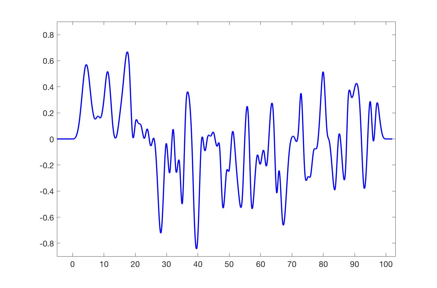
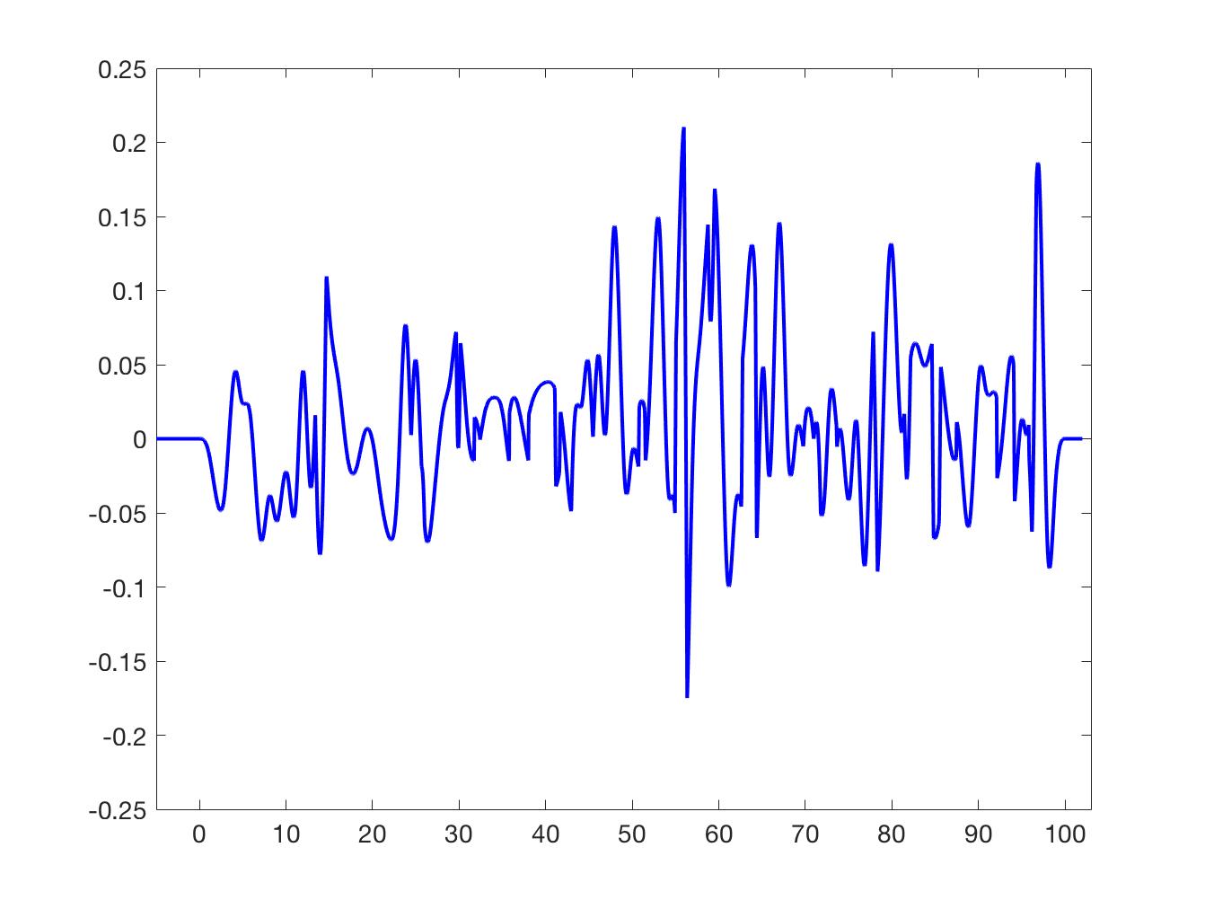
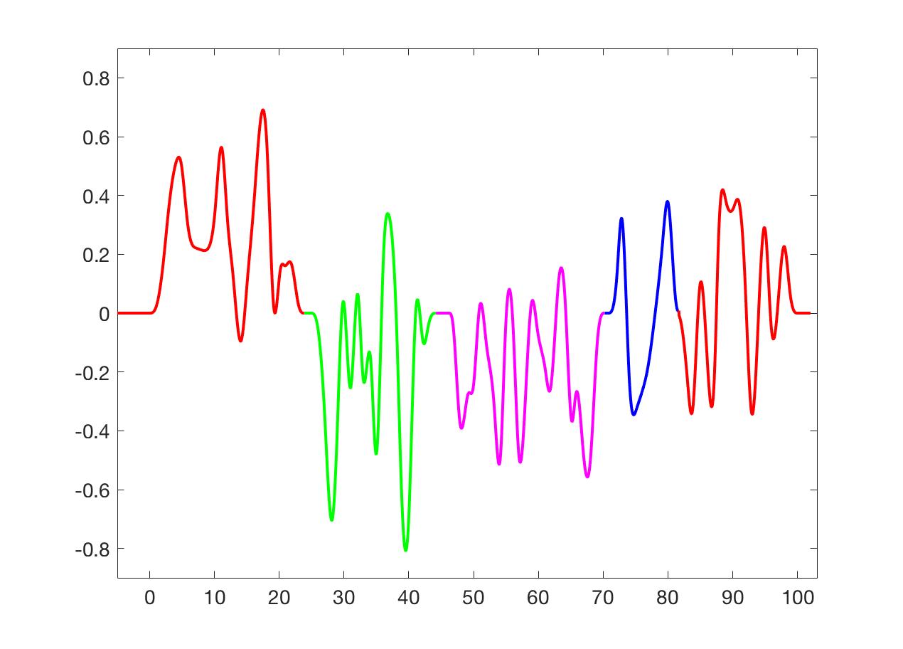
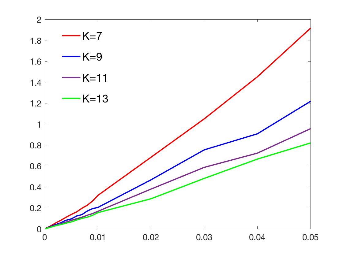
Figure 2. Plotted on the top left is a signal $g_{\eta}$ reconstructed via the proposed MAPS algorithm, while on the top right is the difference $|g_{\eta}|-|f_{o}|$ between magnitude measurements of the reconstructed signal $g_{\eta}$ and the original signal $f_{o}$ plotted on the left of Figure 1. The signal $h_{\eta}$ in Theorem 6.2 is plotted on the bottom left which has five “islands” decomposition (1.4), (1.5) and (1.6). On the bottom right is the average of maximal reconstruction error $E_{\eta,K}$ in 200 trials with respect to different noise levels $\eta$ and oversampling rates $K$.

Performance of the proposed MAPS algorithm depends on the noise level $\eta$ and also the oversampling rate $K$, the ratio between the density $K(b-a)/N$ of the sampling set $\Gamma$ in (7.3) and the rate $(b-a)/N$ of innovation of signals in $V(\Phi)$. Denote by

$$E_{\eta,K}:=\||g_{\eta}|-|f|\|_{\infty}$$

the maximal reconstruction error in magnitude measurements between the original signal $f$ and the reconstructed signal $g_{\eta}$ for different noise levels $\eta$ and oversampling rate $K$. Plotted on the bottom right of Figure 2 are average of the maximal reconstruction error $E_{\eta,K}$ in 200 trials against the noise level $\eta$ and oversampling rate $K$. This indicates that the maximal reconstruction error $E_{\eta,K}$ depends almost linearly on the noise level $\eta$, and decreases as the oversampling rate $K$ increases, cf. (6.17) and Theorem 6.2.

Let $D$ be a triangulation composed by the triangles $T_{\theta},\theta\in\Theta$, and denote the set of all inner nodes of the triangulation by $\Lambda$. In the second simulation, we consider piecewise affine signals

(7.4) $$f(x,y)=\sum_{\lambda\in\Lambda}c_{\lambda}\phi_{\lambda}(x,y)$$

on the triangulation $D$, where the basis signals $\phi_{\lambda},\lambda\in\Lambda$ are piecewise affine on triangles $T_{\theta},\theta\in\Theta$ with $\phi_{\lambda}(\lambda)=1$ and $\phi_{\lambda}(\lambda^{\prime})=0$ for all other nodes $\lambda^{\prime}\neq\lambda$, see the right image of Figure 1. From the definition of basis signals $\phi_{\lambda},\lambda\in\Lambda$, a signal $f$ of the form (7.4) has the following interpolation property,

$$f(x,y)=\sum_{\lambda\in\Lambda}f(\lambda)\phi_{\lambda}(x,y).$$

In the simulation, phaseless samples of a piecewise affine signal $f$ on a discrete set $\Gamma=\cup_{\theta\in\Theta}\Gamma_{\theta}$ are corrupted by the bounded random noise,

(7.5) $${z}_{\eta}({\gamma})=|f({\gamma})|+\eta({\gamma}),\ {\gamma}\in\Gamma,$$

where $\eta(\gamma),\gamma\in\Gamma$, are randomly selected in the interval $[-\eta,\eta]$ for some $\eta\geq 0$ and for every $\theta\in\Theta$, the set $\Gamma_{\theta}$ contains $7$ points randomly selected inside $T_{\theta}$. Shown on the left of Figure 3 is a signal $g_{\eta}$ reconstructed from the noisy phaseless samples (7.5) via the proposed MAPS algorithm, where $\eta=0.01$, the original piecewise affine signal $f$ is plotted on the right of Figure 1, and the maximal reconstruction error $\||g_{\eta}|-|f|\|_{\infty}$ in magnitude measurements between the original signal $f$ and the reconstructed signal $g_{\eta}$ is $0.0360$.

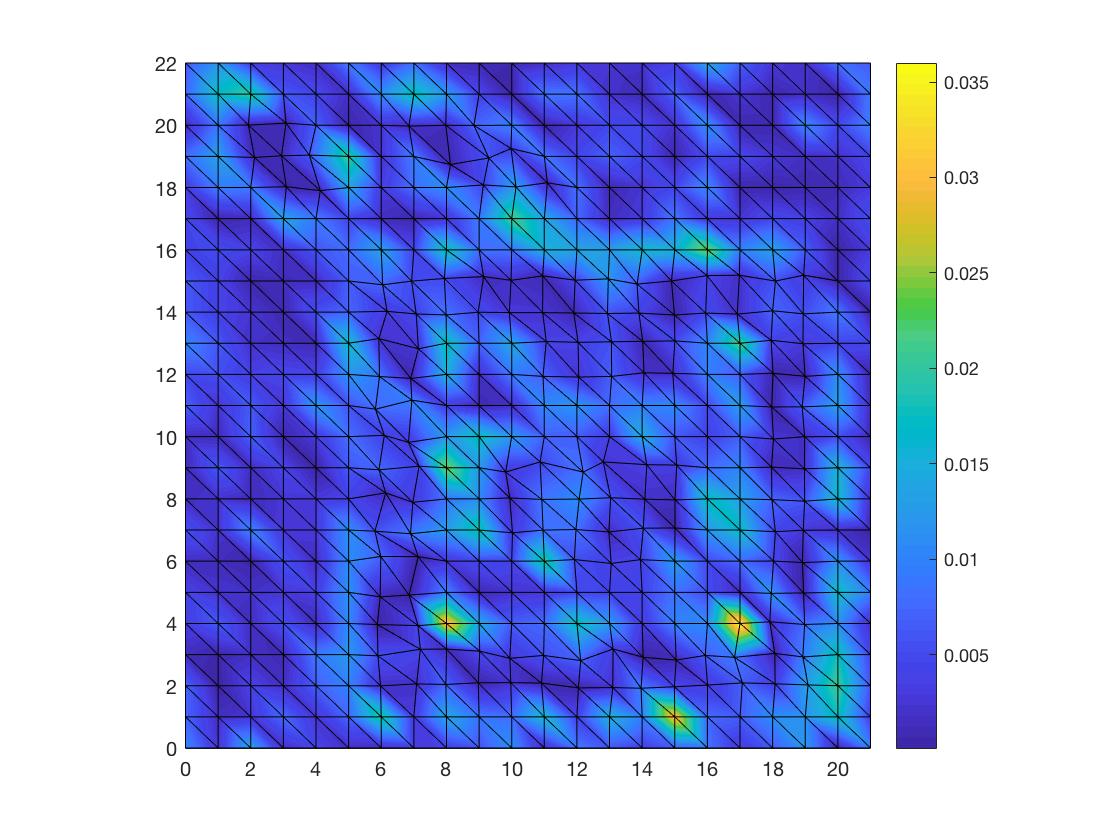
Figure 3. Plotted on the left is a reconstructed signal $g_{\eta}$ via the MAPS algorithm, while on the right is the difference $||g_{\eta}|-|f||$ between magnitude measurements of the reconstructed signal $g_{\eta}$ and the original signal $f$ plotted on the right of Figure 1.

In the simulation, we consider the performance of the proposed MAPS algorithm to construct piecewise affine approximation when the original signal $f$ of the form (7.4) has evaluations $f(\lambda),\lambda\in\Lambda$ on their inner nodes being randomly selected in $[-1,1]$. Denote by $g_{\eta}$ the reconstructed signal from the noisy phaseless samples (7.5) via the proposed MAPS algorithm and let $E_{\eta}:=\||g_{\eta}|-|f|\|_{\infty}$ be the maximal reconstruction error in magnitude measurements between the original signal $f$ and the reconstructed signal $g_{\eta}$ for different noise levels $\eta$. Shown in Table 1 is the average of maximal reconstruction error $E_{\eta}$ in 200 trials. This confirms the conclusion in Theorem 6.2 that the maximal reconstruction error depends almost linearly on the noise level $\eta\geq 0$.

Table 1. Maximal reconstruction error via the MAPS algorithm

$\eta$	0.04	0.03	0.02	0.01	0.008	0.004	0.002	0.001
$E_{\eta}$	0.1878	0.1366	0.0791	0.0305	0.0226	0.0101	0.0050	0.0025

Appendix A Density of phaseless sampling sets

In the appendix, we introduce a necessary condition on a discrete set $\Gamma$ such that ${\mathcal{M}}_{f,\Gamma}={\mathcal{M}}_{f}$ for all $f\in V(\Phi)$. We show that that the density of such a discrete set $\Gamma$ is no less than the innovation rate of signals in $V(\Phi)$, see Theorem A.1 and Corollary A.2.

Theorem A.1.

Let the domain $D$, the generator $\Phi:=(\phi_{\lambda})_{\lambda\in\Lambda}$, the family ${\mathcal{T}}=\{T_{\theta},\theta\in\Theta\}$ of open sets and the linear space $V(\Phi)$ be as in Theorem 3.2. If ${\mathcal{M}}_{f,\Gamma}={\mathcal{M}}_{f}$ for all $f\in V(\Phi)$ with ${\mathcal{M}}_{f}=\{\pm f\}$, then

(A.1) $$D_{+}(\Gamma)\geq D_{+}(\Lambda).$$

Proof.

Take $x\in D$ and $r\geq r_{0}$. By (2.2) and (2.4), it suffices to prove that

(A.2) $$\#(\Gamma\cap B(x,r))\geq\#(\Lambda\cap B(x,r-r_{0})).$$

Assume, on the contrary, that (A.2) does not hold. Then there exists a nonzero vector $(d_{\lambda})_{\lambda\in\Lambda\cap B(x,r-r_{0})}$ such that

(A.3) $$\sum_{\lambda\in B(x,r-r_{0})\cap\Lambda}d_{\lambda}\phi_{\lambda}(\gamma)=0,\ \gamma\in\Gamma\cap B(x,r).$$

Recall that $\phi_{\lambda},\lambda\in\Lambda$, are supported in $B(\lambda,r_{0})$ by Assumption 2.2. Hence

(A.4) $$\sum_{\lambda\in B(x,r-r_{0})\cap\Lambda}d_{\lambda}\phi_{\lambda}(\gamma)=0,\ \gamma\in\Gamma\backslash B(x,r).$$

Therefore the set

$$W=\Big{\{}f:=\sum_{\lambda\in\Lambda\cap B(x,r-r_{0})}c_{\lambda}\phi_{\lambda}:\ f(\gamma)=0,\ \gamma\in\Gamma\Big{\}}\subset V(\Phi)$$

contains nonzero signals. Take a nonzero signal $f\in W$. By Theorem 4.3, $f=\sum_{i\in I}f_{i}$ for some nonzero signals $f_{i}\in V(\Phi),i\in I$, such that ${\mathcal{M}}_{f_{i}}=\{\pm f_{i}\},i\in I$, and $f_{i}f_{i}^{\prime}=0$ for all distinct $i,i^{\prime}\in I$. This together with $f\in W$ implies that $f_{i}(\gamma)=0$ for all $\gamma\in\Gamma$ and $i\in I$. Hence $0\in{\mathcal{M}}_{f_{i},\Gamma},i\in I$, which contradicts with ${\mathcal{M}}_{f_{i},\Gamma}={\mathcal{M}}_{f_{i}}=\{\pm f_{i}\},i\in I$. ∎

From the above argument, we have the following result without the assumption on the family ${\mathcal{T}}$ of open sets in Theorem A.1.

Corollary A.2.

Let the domain $D$ and the generator $\Phi:=(\phi_{\lambda})_{\lambda\in\Lambda}$ satisfy Assumptions 2.1 and 2.2 respectively, and define the linear space $V(\Phi)$ by (2.3). If $\Gamma$ is a discrete set with ${\mathcal{M}}_{f,\Gamma}={\mathcal{M}}_{f}$ for all $f\in V(\Phi)$, then $D_{+}(\Gamma)\geq D_{+}(\Lambda)$.

We finish this appendix with a remark that the low bound in (A.1) can be reached when the generator $\Phi=(\phi_{\lambda})_{\lambda\in\Lambda}$ satisfies that

(A.5) $$S_{\Phi}(\lambda,\lambda^{\prime})=\emptyset\ {\rm for\ all\ distinct}\ \lambda,\lambda^{\prime}\in\Lambda.$$

As in this case, a signal $f\in V(\Phi)$ is nonseparable if and only if $f=c_{\lambda}\phi_{\lambda}$ for some $\lambda\in\Lambda$. Thus the set $\Gamma=\{a(\lambda),\lambda\in\Lambda\}$ is a phaseless sampling set whose upper density is the same as the rate of innovation, where $a(\lambda),\lambda\in\Lambda$, are chosen so that $\phi_{\lambda}(a(\lambda))\neq 0$.

Acknowledgment. The authors thank Professor Ingrid Daubechies for her valuable comments and suggestions in the preparation of the paper.

References

- [1] R. Alaifari, I. Daubechies, P. Grohs, and R. Yin, Stable phase retrieval in infinite dimensions, Arxiv preprint, arXiv:1609.00034
- [2] R. Alaifari and P. Grohs, Phase retrieval in the general setting of continuous frames for Banach spaces, Arxiv preprint, arXiv:1604.03163
- [3] R. Balan, B. G. Bodmann, P. G. Casazza, and D. Edidin, Painless reconstruction from magnitudes of frame coefficents, J. Fourier Anal. Appl., 15(2009), 488–501.
- [4] R. Balan, P. G. Casazza, and D. Edidin, On signal reconstruction without phase, Appl. Comput. Harmon. Anal., 20(2006), 345–356.
- [5] R. Balan, P. G. Casazza, C. Heil, and Z. Landau, Density, overcompleteness and localization of frames I: theory, J. Fourier Anal. Appl., 12(2006), 105-143; II: Gabor system, J. Fourier Anal. Appl., 12(2006), 309–344.
- [6] A. S. Bandeira, J. Cahill, D. G. Mixon, and A. A. Nelson, Saving phase: injectivity and stability for phase retrieval, Appl. Comput. Harmon. Anal., 37(2014), 106–125.
- [7] T. Blu, P. Thevenaz, and M. Unser, Linear interpolation revitalized, IEEE Trans. Image Process., 13(2004), 710–719.
- [8] J. Cahill, P. G. Casazza, and I. Daubechies, Phase retrieval in infinite-dimensional Hilbert spaces, Trans. Amer. Math. Soc., Ser. B, 3(2016), 63–76.
- [9] E. J. Candes, Y. C. Eldar, T. Strohmer, and V. Voroninski, Phase retrieval via matrix completion, SIAM J. Imaging Sci., 6(2013), 199–225.
- [10] E. Candes, T. Strohmer, and V. Voroninski, Phaselift: exact and stable signal recovery from magnitude measurements via convex programming, Comm. Pure Appl. Math., 66(2013), 1241–1274.
- [11] P. G. Casazza, D. Ghoreishi, S. Jose, and J. C. Tremain, Norm retrieval and phase retrieval by projections, Arxiv preprint, arXiv:1701.08014
- [12] P. G. Casazza, The art of frame theory, Taiwanese J. Math., 4(2000), 129–201.
- [13] Y. Chen, C. Cheng, Q. Sun, and H. Wang, Phase retrieval of real-valued signals in a shift-invariant space, Arxiv preprint, arXiv:1603.01592
- [14] C. Cheng, J. Jiang, and Q. Sun, Phaseless sampling and reconstruction of real-valued signals in shift-invariant spaces, Arxiv preprint, arXiv:1702.06443
- [15] C. Cheng, Y. Jiang, and Q. Sun, Spatially distributed sampling and reconstruction, App. Comput. Harmon. Anal., In press.
- [16] D. L. Donoho, Compressed sensing, IEEE Trans. Inf. Theory, 52(2006), 1289– 1306.
- [17] P. L. Dragotti, M. Vetterli, and T. Blu, Sampling moments and reconstructing signals of finite rate of innovation: Shannon meets Strang-Fix, IEEE Trans. Signal Process., 55(2007), 1741 –1757.
- [18] B. Gao, Q. Sun, Y. Wang, and Z. Xu, Phase retrieval from the magnitudes of affine linear measurements, Adv. Appl. Math, 93(2018), 121–141.
- [19] K. Gröchenig, Foundation of Time-Frequency Analysis , Birkhauser, Boston, 2001.
- [20] P. Grohs and M. Rathmair, Stable Gabor phase retrieval and spectral clustering, Arxiv preprint, arXiv: 1706.04374
- [21] D. Han, T. Juste, Y. Li, and W. Sun, Frame phase-retrievability and exact phase-retrievable frames, Arxiv preprint, arXiv:1706.07738
- [22] H. S. Hou and H. C. Andrews, Cubic splines for image interpolation and digital filtering, IEEE Trans. Acoust. Speech Signal Process., 26(1978), 508–517.
- [23] K. Jaganathan, Y. C. Eldar, and B. Hassibi, Phase retrieval: an overview of recent developments, In Optical Compressive Imaging, edited by A. Stern, CRC Press, 2016, 261–296.
- [24] A. J. E. M. Janssen, Duality and biorthogonality for Weyl-Heisenberg frames, J. Fourier Anal. Appl., 1(1995), 403–436.
- [25] R.-Q. Jia and C. A. Micchelli, On linear independence of integer translates of a finite number of functions, Proc. Edinburgh Math. Soc., 36(1992), 69 –75.
- [26] R. A. Macias and C. Segovia, Lipschitz functions on spaces of homogeneous type, Adv. Math., 33(1979), 257 –270.
- [27] S. Mallat and I. Waldspurger, Phase retrieval for the Cauchy wavelet transform, J. Fourier Anal. Appl., 21(2015), 1251–1309.
- [28] V. Pohl, F. Yang, and H. Boche, Phaseless signal recovery in infinite dimensional spaces using structured modulations, J. Fourier Anal. Appl., 20(2014), 1212–1233.
- [29] A. Ron, A necessary and sufficient condition for the linear indepdence of the integer translates of a compactly supported distribution, Constr. Approx., 5(1989), 297–308.
- [30] A. Ron and Z. Shen, Weyl-Heisenberg frames and Riesz bases in , Duke Math. J., 89(1997), 237–282.
- [31] Y. Shechtman, Y. C. Eldar, O. Cohen, H. N. Chapman, J. Miao, and M. Segev, Phase retrieval with application to optical imaging: a contemporary overview, IEEE Signal Proc. Mag., 32(2015), 87–109.
- [32] L. L. Schumaker, Spline Functions: Basic Theory , John Wiley & Sons, New York, 1981.
- [33] B. A. Shenoy, S. Mulleti, and C. S. Seelamantula, Exact phase retrieval in principal shift-invariant spaces, IEEE Trans. Signal Proc., 64(2016), 406–416.
- [34] Q. Sun, Localized nonlinear functional equations and two sampling problems in signal processing, Adv. Comput. Math., 40(2014), 415 –458.
- [35] Q. Sun, Local reconstruction for sampling in shift-invariant space, Adv. Comput. Math., 32(2010), 335–352.
- [36] Q. Sun, Frames in spaces with finite rate of innovation, Adv. Comput. Math., 28(2008), 301–329.
- [37] Q. Sun, Non-uniform average sampling and reconstruction of signals with finite rate of innovation, SIAM J. Math. Anal., 38(2006), 1389–1422.
- [38] W. Sun, Phaseless sampling and linear reconstruction of functions in spline spaces, Arxiv preprint, arXiv:1709.04779
- [39] G. Thakur, Reconstruction of bandlimited functions from unsigned samples, J. Fourier Anal. Appl., 17(2011), 720–732.
- [40] M. Unser, Splines: a perfect fit for signal and image processing, IEEE Signal Proc. Mag., 16(1999), 22–38.
- [41] M. Vetterli, P. Marziliano, and T. Blu, Sampling signals with finite rate of innovation, IEEE Trans. Signal Proc., 50(2002), 1417–1428.
- [42] G. Wahba, Spline Models for Observational Data, CBMS-NSF Regional Conference Series in Applied Mathematics, 59, SIAM, Philadelphia, PA, 1990.
- [43] Y. Wang and Z. Xu, Phase retrieval for sparse signals, Appl. Comput. Harmon. Anal., 37 (2014), 531–544.
- [44] Da. Yang, Do. Yang, and G. Hu, The Hardy Space with Non-doubling Measures and Their Applications, Lecture Notes in Mathematics, Springer, 2013.