ALE: Additive Latent Effect Models for Grade Prediction
Abstract
The past decade has seen a growth in the development and deployment of educational technologies for assisting college-going students in choosing majors, selecting courses and acquiring feedback based on past academic performance. Grade prediction methods seek to estimate a grade that a student may achieve in a course that she may take in the future (e.g., next term). Accurate and timely prediction of students’ academic grades is important for developing effective degree planners and early warning systems, and ultimately improving educational outcomes. Existing grade prediction methods mostly focus on modeling the knowledge components associated with each course and student, and often overlook other factors such as the difficulty of each knowledge component, course instructors, student interest, capabilities and effort.
In this paper, we propose additive latent effect models that incorporate these factors to predict the student next-term grades. Specifically, the proposed models take into account four factors: (i) student’s academic level, (ii) course instructors, (iii) student global latent factor, and (iv) latent knowledge factors. We compared the new models with several state-of-the-art methods on students of various characteristics (e.g., whether a student transferred in or not). The experimental results demonstrate that the proposed methods significantly outperform the baselines on grade prediction problem. Moreover, we perform a thorough analysis on the importance of different factors and how these factors can practically assist students in course selection, and finally improve their academic performance.
1 Introduction.
One of the grand challenges facing higher education institutions, (i.e., four-year colleges/universities and community colleges) is low graduation rates [13]. To increase student graduation rates, several educational data mining techniques have been developed and deployed at several institutions to provide students degree pathways towards successful graduation [18]. Additionally, early warning systems have been developed to monitor student progress, and identify students at-risk of dropping majors or performing below their potential in a given major. An effective way to assist and improve degree planning and advising is via modeling the student’s knowledge and foreseeing their future academic performance [13].
Matrix factorization (MF) based approaches have been widely used for solving the grade prediction problems [19, 3]. MF methods decompose the student-course grade matrix into two low-rank matrices containing student and course latent factors. The prediction of a student’s grade on an untaken course will be calculated as the similarity of the corresponding student latent factors and course latent factors. However, the existing grade prediction methods often have a narrow focus on the potential influential factors. For example, course instructors, course difficulty, student’s interest, capability and effort are rarely considered in the existing methods, which are all important factors to the student’s grades.
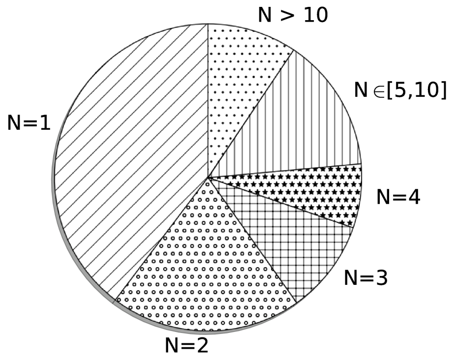
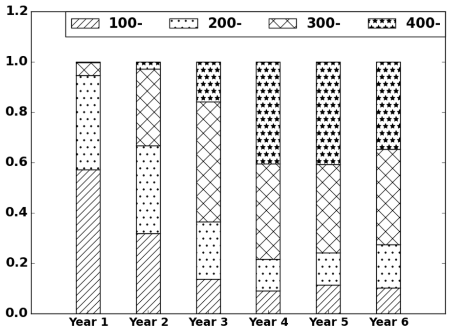
Data distribution: Fig. 1(a) shows the distribution of the number of instructors who teach the same course at George Mason University. More than 60% of the courses at this university have been taught by multiple instructors in a period of 18 terms. For a given course, different instructors differ in their course offerings with respect to coverage of course topics, pedagogy and grading criterion. All these factors impact a student’s grade in a course. As such, we propose to model latent factors associated with each instructor in addition to the latent factors of the course she teaches. Fig. 1(b) shows the distribution of academic course levels at George Mason University (i.e., 100-,200-,300- and 400-level) offered to the students in different starting years. We assume that students in the same college terms (e.g., freshmen, sophomore, etc) tend to have similar learning behaviors, capabilities and expertise given the sequential aspects of most degree programs. For example, freshmen students may be undecided on their majors and mostly take courses with level 100, as shown in Fig.1(b). Likewise, seniors tend to have an in-depth knowledge of study in a specific field, and mostly take higher level courses.
In this work, we propose Additive Latent Effect (ALE) models within the framework of MF to predict the grade that a student is expected to obtain in a course that she may enroll in the next term. Inspired by Morsy et. al. [11], the proposed methods model each student’s latent factors with accumulated knowledge of a sequence of courses taken by the student, jointly with the grade for each course. Furthermore, we incorporate course instructor and student academic level effects along with student global latent factor to enable accurate grade prediction.
We conducted a comprehensive set of experiments on various datasets and provided a thorough analysis on the importance of different factors. Our experimental results show that the proposed methods achieve superior prediction performance on various test datasets for next-term grade prediction.
The main contributions of our work in this paper can be summarized as follows:
-
1.
We propose additive latent effect models that incorporate the information of course instructors, student’s academic level and student global latent factor for the next-term grade prediction problem. The strengths of our proposed framework include the ability to enhance the standard MF methods with additional student and course-specific content information that may not be contained within the student-course grade matrix.
-
2.
We implement a number of extensive experiments on different student groups partitioned by student starting years and student majors. We then provide detailed analysis on the importance of each additive effect in our model, and how to assist students in selecting courses.
2 Related Work.
Over the past few years, a large number of methods influenced by Recommender System (RS) research [1], including Collaborative Filtering (CF) [12] and Matrix Factorization [8] have inspired the development of methods for educational data mining to solve the next-term grade prediction problem [20] and in-class grade prediction problem [4]. For example, Sahebi et. al. [17] modeled student learning progress and predicted student performance using tensor decomposition based on the sequence of student attempts within course quizzes. Lan et. al. [9] predicted student performance on different questions within the context of intelligent tutoring systems. Meier et. al. [10] developed an online learning method that learns the best time to intervene based on past student performance in a course. Additionally, incorporation of biases has shown to be important for several educational data mining problems, following its success in RS [8]. Elbadrawy et. al. [2] developed a domain-aware grade prediction method with student/course-group based biases. To predict student ’ grade on course , this method groups students and courses in different ways based on student majors, academic levels and course subjects, and introduces group-based biases. The key intuition of this method is that students who take the same course and can be grouped by domain information (e.g., student’s major) may share a similar bias.
In educational data mining problems, sequential information of students/courses over time is very common and thus methods that deal with sequential data can be beneficial. As a matter of fact, such methods have been extensively developed in RS research. For example, integrated methods of Markov Chains (MC) and MF have been popular in dealing with sequential data in RS. Rendle et. al. [15] proposed the factorized personalized MC models. These models have personalized Markov chains that rely on transition matrices, and these methods use a factorization model to deal with the sparsity in the input data. He et. al. [6] developed factorized sequential models with item similarities for sparse sequential recommendation. Their models consider both long-term and short-term dynamics among user-item data. He et. al. [5] adopted a similar idea and developed large-scale recommender systems to model the preferences and short-term dynamics between both users and items.
Prior work in the RS literature that shares similarities with our proposed method is from Koenigstein et. al. [7]. In this work, the authors proposed a music rating recommendation system that models a user’s music preferences based on her interest in a given music track, and the artist and album information associated with the specific track. Shared factor components were introduced to reflect the similar preference for music tracks of same artists (or genre, album).
3 Notations and Definitions
Formally, student-course grades will be represented by {, , …, } for terms. contains the set of tuples storing grade information for all students enrolled in courses within term . Each tuple stores: (i) student identifier, (ii) course identifier, (iii) student academic level, (iv) course instructor, and (v) grade obtained. For all students, the student-course grades up to the term can be represented by =. The set of courses that student has taken in term is represented by and the grades that student achieves in term is represented by . The set of courses that student has taken up to term is represented by , and the grades that student has achieved up to term is represented by .
In this paper, all vectors (e.g., and ) are represented by bold lower-case letters and all matrices (e.g., ) are represented by upper-case letters. Row vectors are represented by having the transpose superscriptT, otherwise by default they are column vectors. A predicted value is denoted by having a symbol. Table 1 summarizes the key notations used in this paper.
Given student-course grades up to term , the objective of the next-term grade prediction problem is to predict grades for each student on courses that the student may consider for enrollment in the next term .
| Notation | Explanation |
| number of courses | |
| number of students | |
| the dimension of latent factors | |
| latent factors of accumulated knowledge of student | |
| up to term | |
| latent factor of student ’s academic level, | |
| integrated student latent factor | |
| latent factor of the knowledge components required | |
| by course | |
| latent factor of the instructor who teaches course | |
| integrated course latent factor | |
| student ’s global latent factor | |
| latent factor of the knowledge components provided | |
| by course | |
| student-course grades at term | |
| all the student-course grades up to term | |
| the grade of student on course at term | |
| the set of courses student chooses at term | |
| the set of courses student chooses up to term | |
| all the grades student obtains at term | |
| all the grades student obtains up to term | |
| the academic term when student takes course |
4 Background and Prior Methods
4.1 Matrix Factorization Based Grade Prediction
Matrix factorization from RS [16] can be applied for the next-term grade prediction problem, when the student-course grade matrix is considered as the user-item rating matrix. Two low-rank matrices containing latent factors of courses and students in a common knowledge space can be learned from such a student-course grade matrix [19]. Thus, the grade of a student on a course can be predicted as
| (4.1) |
where () and () are the two vectors containing latent factors of dimensions for student and course , respectively. This method is denoted as MF.
Including the bias terms within the MF formulation has shown to be effective in modeling systematical biases [8]. For the grade prediction problem using MF, student and course biases can be included as follows:
| (4.2) |
where and are bias terms for student and course , respectively. This method is referred to as MF with bias terms and denoted as MF-b.
4.2 MF with Domain-Aware Biases
El-Badrawy et. al. developed a domain-aware MF based methods for the next-term grade prediction problem [2]. These methods involve group-specific bias within MF formulation. Groups are defined based on student- and course-specific information.
In this method, the grade for student on course is predicted as:
| (4.3) |
where () and () are the latent factors for student and course , respectively. denotes the grouping information. is the bias term for course . This method models course bias based on the performance of students who are in the same group of student (i.e., ) and have taken course before. Similarly, is the student bias term modeled based on the grades student has got on the courses which are in the same group as course (i.e., ). We refer to this method as MF with domain-aware biases and denote it as MF-d.
4.3 Cumulative Knowledge-based Regression Models
Morsy et. al. [11] consider the series of courses a student takes as a sequence and propose Cumulative-Knowledge Regression Models (CKRM). Specifically, to predict student ’s performance on course , CKRM represents student with the series of courses she has taken in the past, and each course is represented by a vector which is expected to capture the latent knowledge components provided by the course. Moreover, CKRM represents course with a vector which is expected to capture the latent knowledge components required by the course. Consequently, given a student in term , is the cumulative knowledge acquired until term , and is given by:
| (4.4) |
where is the term in which student took course , is an exponential time decay function, contains the latent knowledge factors of course , and is the grade of student on course . The grade of student on course is then predicted as follows:
| (4.5) |
In this study, we average the results in Eq 4.5 with the sum of exponential time decay weight, that is:
| (4.6) |
This method is referred to as Averaged CKRM and denoted as ACK. Our preliminary experiments demonstrate that ACK outperforms CKRM.
5 Additive Latent Effect Models (ALE)
We propose Additive Latent Effect (ALE) models to predict student ’s performance on course in term . We will give a thorough presentation on how we model each effect in the following sections.
5.1 Student Academic Level Effect
Based on our assumption that students on a same academic level (i.e., freshmen, sophomore, junior and senior) have a similar level of academic maturity, experience, habits and knowledge, we model student by integrating a factor associated to the college term she is attending, denoted as , into the student accumulated knowledge factors. The integrated student latent factor is denoted as , and is given as follows:
| (5.7) |
where is calculated by Eq 4.6, and represents the academic level of student in term , defined as . Since most students finish college in 4-6 years (8-12 terms), is in . We include -norm regularization on to enforce sparsity on this representation. This is because aims to capture the academic factors (e.g., academic maturity), and student is only able to hold a part of them on a particular academic level (e.g., student cannot be both mature and immature at the same time).
5.2 Course Instructor Effect
Consider that a single course is often taught by multiple instructors who usually vary in their coverage of materials (topics), pedagogy, use of teaching technology, choice of assignments and grading criterion. We hypothesize that a student’s performance on a specific course is greatly influenced by the instructor who teaches her the course. Specifically, for a course , we add a factor associated with the specific instructor who teaches course , denoted as , to the original knowledge latent factors of course . The integrated course latent factor is denoted by , and is given as follows:
| (5.8) |
where denotes the instructor who teaches course . For , we include -norm regularization to control its sparsity. We assume that an instructor is generally proficient only in certain topics (and knowledge components), but not all.
With the course instructor information and student academic level information as proposed above, the grade prediction for student on course is given as follows:
| (5.9) |
5.3 Student Global Latent Factor
Eq. 5.9 captures student knowledge factors per term and captures the sequential dynamics in student’s knowledge state over terms. This can be considered as a latent factor model localized by term. We propose to incorporate a term-agnostic global latent factor that captures the student-course performance interaction. We introduce an additional latent factor that captures the student’s implicit information (e.g., student interest and subject matter mastery toward each knowledge component) in a common latent space as course knowledge components. The estimated grade of student on course at term with this global latent factor is given as:
| (5.10) |
Here, we compute the dot product of and instead of and in this step. The exclusive norm for controls its sparsity since we assume most students have a tendency to perform well in a fraction of the represented knowledge states. We refer to this model as Additive Latent Effect (ALE).
5.4 Student and Course Bias Effect
Inspired by the success of MF methods with bias terms [8], we add student-specific and course-specific bias terms denoted by and within the ACK and ALE formulation in Eq 4.6 and 5.10, respectively, as follows:
| (5.11) |
and
| (5.12) |
We denote the ACK with bias terms as ACK-b, and ALE with bias terms as ALE-b.
Table 2 summarizes the proposed methods and comparative baselines in terms of their key features and effect-components considered in this study.
| Method | Prediction Formulation | Property | ||||
| Baselines | MF | (Eq. 4.1) | ✗ | ✗ | ✗ | ✗ |
| MF-b | (Eq. 4.2) | ✗ | ✗ | |||
| MF-d | (Eq. 4.3) | ✗ | ✗ | |||
| ACK | (Eq. 4.6) | ✗ | ✗ | ✗ | ||
| ACK-b | (Eq. 5.11) | ✗ | ||||
| Proposed | ALE | ✗ | ✗ | |||
| Methods | (Eq. 5.10) | |||||
| ALE-b | ALE (Eq. 5.12) | |||||
-
“” indicates the method contains the corresponding property, and “✗” indicates the opposite. indicate student academic level, course instructor and student global latent factor, respectively. and denote student and course bias terms.
5.5 Optimization for ALE
The optimization problem for ALE can be formulated as follows:
| (5.13) |
where represents model parameters (i.e., the latent factors), is the loss function and is the regularization function. We use a squared error loss function in ALE:
| (5.14) |
The is defined as follows:
| (5.15) |
We use stochastic gradient descend (SGD) to solve the optimization problem. The optimization algorithm is presented in Algorithm 1.
5.6 Computational Complexity Analysis
The computational complexity of ALE is determined by the steps from line 6 to line 21 in Algorithm 1. In detail, the computational complexity for line 9 and line 10 is upper-bounded by , where is the maximum number of courses that a student can take in college. For line 11 and line 12, the computational complexity is . Line 13 and line 15 have complexity as well. From line 16 to line 20, the total computational complexity is . Thus, the computational complexity for ALE is , where is the number of iterations, is the total number of student-course grades, is the maximum number of courses that a student can take, and is the dimension of latent factors. Typically, and thus the complexity is .
6 Experiments
6.1 Dataset Description
We evaluated our methods on student grade data obtained from George Mason University. The data was extracted in the period of Fall 2009 to Spring 2016 and includes information for 23,013 transfer students (TR) and 20,086 first-time freshmen (FTF; i.e., students who begin their study at George Mason University) across 151 majors enrolled in 4,654 courses for both TR and FTF students.
Specifically, we evaluated the proposed models on nine large and diverse majors including: (i) Mathematical Sciences (MATH), (ii) Physics (PHYS), (iii) Chemistry (CHEM) (iv) Computer Science (CS), (v) Civil, Environmental and Infrastructure Engineering (CEIE), (vi) Biology (BIOL), (vii) Psychology (PSYC), and (viii) Applied Information Technology (AIT). Table 3 presents the details about these majors.
| Major | FTF Students | TR Students | ||||
| #S | #C | #S-C | #S | #C | #S-C | |
| MATH | 209 | 84 | 2,846 | 258 | 91 | 2,580 |
| PHYS | 127 | 53 | 1,830 | 74 | 48 | 854 |
| CHEM | 342 | 55 | 4,649 | 278 | 66 | 3,105 |
| CS | 988 | 76 | 13,809 | 554 | 68 | 7,028 |
| CEIE | 428 | 80 | 6,925 | 248 | 92 | 4,036 |
| BIOL | 1,629 | 109 | 21,519 | 1,525 | 115 | 16,615 |
| PSYC | 1,114 | 95 | 14,377 | 1,749 | 114 | 18,939 |
| AIT | 334 | 82 | 6088 | 1,170 | 90 | 15,060 |
| Total | 5,171 | 634 | 72,043 | 5,856 | 684 | 68,216 |
-
#S, #C and #S-C are number of students, courses and student-course grades from Fall 2009 to Spring 2016, respectively.
6.2 Experimental Protocols
To assess the performance of the next-term grade prediction models, we train our models on data up to term and make predictions for term . We evaluate our methods for three test terms, i.e., Spring 2016, Fall 2015 and Spring 2015. As an example, to evaluate predictions for term Fall 2015, data from Fall 2009 to Spring 2015 are used for model training and data from Fall 2015 are used as the test data.
6.3 Parameter Learning
The parameters in the optimization problem (Eq 5.15) contain the number of latent dimensions (i.e., ), regularization weights (i.e., , , ), and time decay parameter (i.e., ). We use a validation set to select parameters. Specifically, for test term , we have student-course grades up to term as the training set, i.e., . Then we split the training set into two parts: and , the latter of which we consider as the validation set. We did a grid search over the parameters and selected the parameters that perform best on the validation set.
6.4 Evaluation Metrics
In our dataset, a student’s grade is a letter grade (i.e. A, A-, …, F). As done previously in Polyzou et. al. [14], we compute the Percentage of Tick Accuracy (PTA). First, we define a tick as the difference between two consecutive letter grades (e.g., C+ vs C or C vs C-). To assess the performance of our grade prediction methods, we convert the predicted numerical grades into their closest letter grades. Specifically, we set letter grade “A+” and “A” correspond to number 4.0, “A-” correspond to number 3.67, “B+” correspond to number 3.33, etc. In our experiments, we first convert letter grades to numbers during training, and then convert the predicted numbers to letter grades during testing and compute the percentage of predicted grades with no error (or 0-ticks), within 1 tick and within 2 ticks denoted by PTA0, PTA1 and PTA2, respectively. For course selection and degree planning purposes, courses predicted within 2 ticks can be considered sufficiently close.
We use Mean Absolute Error (MAE) for evaluating the predicted results with numbers. MAE is given as:
| (6.16) |
where and are the ground truth and predicted grade for student on course , respectively. is the test set of (student, course, grade) triples in the -th term.
| Method | FTF - Spring 2016 | TR - Spring 2016 | |||||||||||||
| parameters | MAE | PTA0 | PTA1 | PTA2 | parameters | MAE | PTA0 | PTA1 | PTA2 | ||||||
| \hlineB1 MF | 10 | – | – | 0.723 | 0.188 | 0.338 | 0.580 | 10 | – | – | 0.706 | 0.188 | 0.341 | 0.601 | |
| MF-b | 10 | – | – | 0.670 | 0.206 | 0.360 | 0.609 | 10 | – | – | 0.658 | 0.226 | 0.387 | 0.628 | |
| MF-d | 5 | – | – | 0.661 | 0.221 | 0.381 | 0.621 | 10 | – | – | 0.683 | 0.216 | 0.366 | 0.614 | |
| ACK | 5 | 0.01 | – | 0.674 | 0.216 | 0.362 | 0.604 | 5 | 0.01 | – | 0.680 | 0.225 | 0.369 | 0.597 | |
| ACK-b | 5 | 0.01 | – | 0.647 | 0.218 | 0.379 | 0.625 | 5 | 0.01 | – | 0.658 | 0.227 | 0.387 | 0.627 | |
| ALE | 0.01 | 0.01 | 0.1 | 0.625 | 0.255 | 0.416 | 0.651 | 0.01 | 0.001 | 0.1 | 0.645 | 0.247 | 0.395 | 0.651 | |
| ALE-b | 0.1 | 0.01 | 0.1 | 0.625 | 0.225 | 0.389 | 0.648 | 0.01 | 0.1 | 0.01 | 0.642 | 0.231 | 0.389 | 0.637 | |
| Method | FTF - Fall 2015 | TR - Fall 2015 | |||||||||||||
| parameters | MAE | PTA0 | PTA1 | PTA2 | parameters | MAE | PTA0 | PTA1 | PTA2 | ||||||
| \hlineB1 MF | 10 | – | – | 0.730 | 0.177 | 0.317 | 0.574 | 10 | – | – | 0.692 | 0.183 | 0.347 | 0.599 | |
| MF-b | 10 | – | – | 0.691 | 0.205 | 0.360 | 0.605 | 10 | – | – | 0.653 | 0.213 | 0.378 | 0.631 | |
| MF-d | 10 | – | – | 0.693 | 0.216 | 0.370 | 0.610 | 10 | – | – | 0.670 | 0.205 | 0.362 | 0.630 | |
| ACK | 5 | 0.01 | – | 0.706 | 0.193 | 0.347 | 0.585 | 5 | 0.01 | – | 0.665 | 0.210 | 0.372 | 0.616 | |
| ACK-b | 5 | 0.01 | – | 0.690 | 0.195 | 0.351 | 0.603 | 5 | 0.01 | – | 0.642 | 0.227 | 0.394 | 0.641 | |
| ALE | 0.1 | 0.001 | 0.05 | 0.654 | 0.251 | 0.400 | 0.638 | 0.01 | 0.001 | 0.05 | 0.615 | 0.243 | 0.418 | 0.670 | |
| ALE-b | 0.01 | 0.01 | 0.1 | 0.660 | 0.223 | 0.379 | 0.634 | 0.01 | 0.01 | 0.1 | 0.627 | 0.216 | 0.392 | 0.655 | |
| Method | FTF - Spring 2015 | TR - Spring 2015 | |||||||||||||
| parameters | MAE | PTA0 | PTA1 | PTA2 | parameters | MAE | PTA0 | PTA1 | PTA2 | ||||||
| \hlineB1 MF | 10 | – | – | 0.760 | 0.168 | 0.306 | 0.547 | 10 | – | – | 0.743 | 0.169 | 0.316 | 0.559 | |
| MF-b | 10 | – | – | 0.718 | 0.186 | 0.335 | 0.582 | 10 | – | – | 0.688 | 0.218 | 0.368 | 0.607 | |
| MF-d | 10 | – | – | 0.716 | 0.215 | 0.358 | 0.595 | 10 | – | – | 0.693 | 0.229 | 0.383 | 0.618 | |
| ACK | 5 | 0.01 | 0.01 | 0.712 | 0.192 | 0.332 | 0.579 | 5 | 0.01 | 0.01 | 0.705 | 0.214 | 0.357 | 0.589 | |
| ACK-b | 5 | 0.01 | 0.01 | 0.690 | 0.203 | 0.354 | 0.599 | 5 | 0.01 | 0.01 | 0.688 | 0.207 | 0.354 | 0.606 | |
| ALE | 0.01 | 0.001 | 0.1 | 0.649 | 0.244 | 0.403 | 0.639 | 0.01 | 0.001 | 0.1 | 0.644 | 0.254 | 0.417 | 0.647 | |
| ALE-b | 0.01 | 0.01 | 0.1 | 0.657 | 0.214 | 0.372 | 0.618 | 0.1 | 0.01 | 0.01 | 0.653 | 0.226 | 0.383 | 0.631 | |
-
Columns under “parameters” indicate different model parameters for the corresponding methods. Specifically, for MF, MF-b and MF-d, the parameter is the dimension of latent factors, (). For ACK and ACK-b, the parameters are the dimension of latent factors, (), and time-decay coefficient, (). For ALE and ALE-b, the parameters are time-decay coefficient, (), regularization weight for and , (), and regularization weight for , (). Bold numbers are the best performing results. In our experiments, we select the best performance for all baseline methods.
7 Results and Discussion
7.1 Overall Performance
Table 4 shows the comparison of MAE and PTA results for FTF and TR students across Spring 2016, Fall 2015 and Spring 2015 test terms. The parameters are determined as discussed in Section 6.3. In our reported results, MF-d [2] has nine different combinations for student- and course-level groupings and has bias. We tried all the proposed combinations and report the best performance among all the results. The results show that ALE has the best performance on all the evaluation metrics (the only exception is in Spring 2016 on MAE). Specifically, ALE outperforms the baseline methods on PTA0, PTA1 and PTA2 by 10.61%, 7.17% and 4.50%, respectively. We also observe that the improvement in performance of ALE over the baseline approaches is greater for Spring 2015 in comparison to Spring 2016, even though the training set for Spring 2015 is smaller than Spring 2016. This shows that ALE can overcome the scarcity issues in a dataset and yield good prediction performance.
7.2 Effects of Bias Terms
For all the datasets in Table 4, MF-b (i.e., MF with student/course-specific bias terms) and MF-d (i.e., MF with domain-aware biases) always outperform MF (i.e., MF without bias terms). In addition, MF-b achieves better PTA0 on TR students, but worse PTA0 on FTF students than MF-d. This is probably because the FTF students show consistent characteristics in comparison to TR students, who typically have more diverse backgrounds.
In Table 4, we also observe that ACK-b consistently outperforms ACK, similar to the comparison between MF-b and MF, but ALE always outperforms ALE-b. This may indicate that the additive latent effects in ALE have also captured the student and course bias information in ALE-b. The results in Table 4 demonstrate that ALE is able to achieve better prediction performance without explicitly modeling student and course biases.
7.3 Importance of Additive Latent Effects
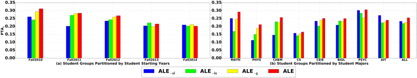
In order to learn the importance of each additive latent effect, we perform a study to assess the prediction performance of different ALE models with a particular latent effect removed. Table 5 shows the details of the compared models in this experiment. Fig. 2 represents the PTA0 performance of each ALE model variant. We test the results on various student groups partitioned by student starting years and student majors, as shown in Fig. 2a and Fig. 2b, respectively. We also implement the experiment for the whole test set, i.e. , and present the results with label “ALL” in Fig. 2b.
| Method | Prediction Formulation | Property | ||
| ALE¬al | ✗ | |||
| ALE¬in | ✗ | |||
| ALE¬g | ✗ | |||
| ALE | ||||
| (Eq. 5.10) | ||||
-
, and indicate the property of student academic level, course instructor and student global latent factor, respectively. indicates the model contains the corresponding property, ✗ indicates the opposite.
Fig. 2 shows that for most student groups, ALE outperforms the other models, indicating that each additive latent effect plays an important role in ALE. Specifically, Fig. 2a shows that for students who start school in Fall 2011, the PTA0 of ALE¬al (without the academic level) drops the most compared to other models. This shows that the student academic level is the most important effect for this student group. Moreover, for students who start school in Fall 2013 and Fall 2014, ALE does not outperform all the other models. This indicates that for these two student groups, it is not necessary to consider all the latent effects when predicting their grades.
From Fig. 2b, we notice that for students in MATH, CS and AIT major, ALE¬in has the worst PTA0 results, indicating the course instructor associated latent factor is the most important for grade prediction. While, for students in PHYS, CHEM and BIOL majors, student academic level is the most important effect. Moreover, Fig. 2b also shows that for all the students (“ALL”), course instructor and student global latent factor are more important than student academic level effect. The ALE outperforms the other three variants. For students with different majors and academic levels, all three effects are important in providing an accurate grade prediction.
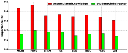
7.4 Importance of Accumulated Knowledge and Student Global Latent Factor
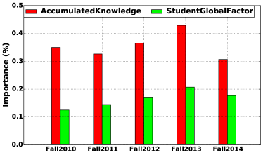
Students need help in course selections both in order to gain course credits and learn the knowledge and skills contained in the course. In ALE, accumulated knowledge and student global latent factor are the two effects that are directly related to the students. Learning the importance of these two factors can assist students when they choose a course.
Specifically, we calculate the importance of each factor by averaging the proportion of its contribution in all the predicted grades within the test set as follows:
| (7.17) |
and
| (7.18) |
where and represent the importance of accumulated knowledge and student global latent factor, respectively.
We present this experiment on students partitioned by starting years and student majors in Fig. 3. For all student groups, accumulated knowledge is always more important than student global latent factor. Specifically, Fig. 3(a) shows that for students who start school in Fall 2013, the proportion of accumulated knowledge is the highest among all student groups and it is the lowest for students who start school in Fall 2014. Moreover, for students who start school in Fall 2010, the proportion of student global latent factor is the lowest among all student groups. We also notice that the difference between the two factors is the smallest for students who start school in Fall 2014. Fig. 3(b) shows the results for student groups partitioned by student majors. It shows that accumulated knowledge is more important than student global latent factor for MATH and PHYS majors. AIT has the smallest difference between accumulated knowledge and student global latent factor.
Based on the results of this experiment, students can balance the course knowledge and their own capabilities when selecting courses. For example, CS students who start school in Fall 2013 have the reference information that about 40% and 20% of their grades are influenced by the accumulated knowledge and student global latent factor, respectively.
8 Conclusion and Future Work
In this paper, we presented additive latent effect models, which incorporate additive latent effects associated with students and courses to solve the next-term grade prediction problem. Specifically, we were able to highlight the improved performance of ALE with use of latent factors of course instructors, student academic levels and student global latent effect. Our experimental results demonstrate that ALE outperforms all the state-of-the-art baselines in various experiments. Specifically, ALE model outperforms the best results among baselines for PTA0, PTA1 and PTA2 by 10.61%, 7.17% and 4.50%, respectively. Moreover, we implemented different sets of experiments to analyze the importance of different effects contained in ALE.
In the future, we plan to add more factors, such as student’s interests and diligence, and build a degree planner which can directly recommend courses to students based on these factors. We hope such a recommender system can not only help students finish their study at college but also guide them plan for careers in the future.
Acknowledgment
Thanks to NSF Big Data Grant #1447489 and GMU IRR Staff for providing data.
References
- [1] Charu C. Aggarwal. Recommender Systems: The Textbook. Springer Publishing Company, Incorporated, 1st edition, 2016.
- [2] Asmaa Elbadrawy and George Karypis. Domain-aware grade prediction and top-n course recommendation. Boston, MA, Sep, 2016.
- [3] Asmaa Elbadrawy, Agoritsa Polyzou, Zhiyun Ren, Mackenzie Sweeney, George Karypis, and Huzefa Rangwala. Predicting student performance using personalized analytics. Computer, 49(4):61–69, 2016.
- [4] Asmaa Elbadrawy, Scott Studham, and George Karypis. Personalized multi-regression models for predicting students performance in course activities. UMN CS, pages 14–011, 2014.
- [5] Ruining He, Chen Fang, Zhaowen Wang, and Julian McAuley. Vista: A visually, socially, and temporally-aware model for artistic recommendation. arXiv preprint arXiv:1607.04373, 2016.
- [6] Ruining He and Julian McAuley. Fusing similarity models with markov chains for sparse sequential recommendation. arXiv preprint arXiv:1609.09152, 2016.
- [7] Noam Koenigstein, Gideon Dror, and Yehuda Koren. Yahoo! music recommendations: modeling music ratings with temporal dynamics and item taxonomy. In Proceedings of the fifth ACM conference on Recommender systems, pages 165–172. ACM, 2011.
- [8] Yehuda Koren, Robert Bell, and Chris Volinsky. Matrix factorization techniques for recommender systems. Computer, 42(8):30–37, August 2009.
- [9] Andrew Lan, Tom Goldstein, Richard Baraniuk, and Christoph Studer. Dealbreaker: A nonlinear latent variable model for educational data. In Proceedings of The 33rd International Conference on Machine Learning, pages 266–275, 2016.
- [10] Yannick Meier, Jie Xu, Onur Atan, and Mihaela van der Schaar. Personalized grade prediction: A data mining approach. In Data Mining (ICDM), 2015 IEEE International Conference on, pages 907–912. IEEE, 2015.
- [11] Sara Morsy and George Karypis. Cumulative knowledge-based regression models for next-term grade prediction. In Proceedings of the 2017 SIAM International Conference on Data Mining, pages 552–560. SIAM, 2017.
- [12] Xia Ning, Christian Desrosiers, and George Karypis. A comprehensive survey of neighborhood-based recommendation methods. In Recommender Systems Handbook, pages 37–76. 2015.
- [13] Michelle Parker. Advising for retention and graduation. 2015.
- [14] Agoritsa Polyzou and George Karypis. Grade prediction with models specific to students and courses. International Journal of Data Science and Analytics, 2(3-4):159–171, 2016.
- [15] Steffen Rendle, Christoph Freudenthaler, and Lars Schmidt-Thieme. Factorizing personalized markov chains for next-basket recommendation. In Proceedings of the 19th international conference on World wide web, pages 811–820. ACM, 2010.
- [16] Francesco Ricci, Lior Rokach, Bracha Shapira, and Paul B Kantor. Recommender systems handbook., 2011.
- [17] Shaghayegh Sahebi, Yu-Ru Lin, and Peter Brusilovsky. Tensor factorization for student modeling and performance prediction in unstructured domain. In Proceedings of the 9th International Conference on Educational Data Mining, pages 502–506. IEDMS, 2016.
- [18] Jill M Simons. A National Study of Student Early Alert Models at Four-Year Institutions of Higher Education. ERIC, 2011.
- [19] Mack Sweeney, Jaime Lester, and Huzefa Rangwala. Next-term student grade prediction. In Big Data (Big Data), 2015 IEEE International Conference on, pages 970–975. IEEE, 2015.
- [20] Nguyen Thai-Nghe, Lucas Drumond, Artus Krohn-Grimberghe, and Lars Schmidt-Thieme. Recommender system for predicting student performance. Procedia Computer Science, 1(2):2811–2819, 2010.