Estimate of the energy spectrum of the light component of cosmic rays in HAWC using the shower age and the fraction of hit PMT’s

Abstract:

The High Altitude Water Cherenkov (HAWC) observatory is a ground-based air-shower detector designed to study the TeV gamma and cosmic ray windows. The observatory is composed of a densely packed array of $300$ water Cherenkov tanks, $4.5$ m deep and $7.3$ diameter with $4$ photomultipliers (PMT) each, distributed on a $22,000\,\mbox{m}^{2}$ surface. The instrument registers the number of hit PMT’s as well as the timing information and the total charge seen by the photomultipliers during the shower event. From the analysis of these data, shower observables such as the arrival direction, the core position at ground, the age and the primary energy are estimated, from which the energy spectrum of cosmic rays and its composition can be studied. In this work, we will describe the methodologies of HAWC cosmic ray analyses, including the Bayesian spectral unfolding procedure used to determine the all-particle and the light component energy spectra of cosmic rays. We will see that the distribution of the shower age vs the fraction of hit PMT’s contains information about the composition of cosmic rays.

1 Introduction

The energy region between $10\,\mbox{TeV}$ and $1\,\mbox{PeV}$ of the cosmic ray spectrum has been poorly explored as it is located at the frontier between the direct and indirect measurements. However, it is of great interest due to the possible presence of new structures in the all-particle and the elemental spectra of cosmic rays as predicted, for example, in [1] or as the recent measurements performed by ARGO-YBJ seem to suggest, which indicate the possible presence of a knee around $1\,\mbox{PeV}$ in the spectrum of the light mass group (H+He) of cosmic rays [2]. HAWC can contribute to the study of both the spectrum and composition of cosmic rays in this poorly explored energy interval. HAWC is an extensive air shower (EAS) observatory located at $4100\,\mbox{m}$ a.s.l. ($\sim 640\,\mbox{g}/\mbox{cm}^{2}$ of atmospheric depth) on the northern slope of the volcano Sierra Negra in Mexico. The instrument is designed to detect $\gamma$ rays in the $100\,\mbox{GeV}$ to $100\,\mbox{TeV}$ energy range, but its altitude and physical dimensions permit measurements of primary hadronic cosmic rays up to PeV energies. In this contribution, we will describe analyses that are underway to determine the spectra of the all-particle and the light component of cosmic rays using HAWC data.

2 Event reconstruction and simulation

HAWC is composed of $300$ water Cherenkov detectors, $4.5$ m deep and $7.3$ m in diameter, each instrumented with $4$ upward-facing photomultipliers (PMTs). The instrument covers a $22,000\,\mbox{m}^{2}$ area and registers the PMT signals and their respective timing information from extensive air-showers [3]. From these data, the event reconstruction procedure allows estimation of various shower properties such as the arrival direction, the core position at ground-level, the lateral shower age parameter (hereafter referred to as age) and the primary energy.

For a primary particle interacting in the atmosphere, the resulting air shower is simulated using the CORSIKA [4] package (v740), with FLUKA [5], and QGSJet-II-03 [6] as the hadronic interaction models. Primaries of the eight species measured by the CREAM [9] flights (H, ⁴He, ¹²C, ¹⁶O, ²⁰Ne, ²⁴Mg, ²⁸Si, ⁵⁶Fe) were generated on an $E^{-2}$ differential energy spectrum from 5 GeV $-$ 3 PeV and distributed over a 1 km radius circular throwing area. The simulated zenith angle range was $0^{\circ}-70^{\circ}$, azimuthally symmetric, and weighted to a $\sin{\theta}\cos{\theta}$ arrival distribution, where $\theta$ is the zenith angle of the shower axis. The secondary charged particles interacting with the HAWC detector were simulated using the GEANT4 [7] package. Dedicated HAWC software was used to simulate the detector response over the entire hardware and data analysis chain. Simulations for each particle type are re-weighted to the best fits of a broken power-law to data from direct-detection measurements provided by AMS [8], CREAM [9], and PAMELA [10], constituting our nominal composition model.

The age, $s$, is obtained event-by-event from a fit to the lateral charge distribution measured by the PMT’s at the shower plane with an NKG function [11]:

$$f_{ch}(r)=A\cdot(r/r_{0})^{s-3}\cdot(1+r/r_{0})^{s-4.5},$$ (1)

where $r$ is the radial distance to the shower axis, $r_{0}=124.21\,\mbox{m}$ is the Moliere radius and $A$ is a normalization parameter. This lateral distribution function gives a good description of gamma-induced EAS [12], and a reasonable description of hadron-induced showers at energies $E\lesssim 50$ TeV. At higher energies and large core distances, however, deviations appear between the above function and the observed lateral distribution of showers produced by cosmic rays. Further research to reduce these differences is now ongoing and will serve to improve the preliminary composition analysis that is presented here.

(a)

(b)

(c)

Figure 1: Bias distribution for the bin centered at $E_{\textnormal{true}}=100$ TeV (left), showing the definitions of energy bias, resolution, and efficiency. The Monte Carlo values are indicated by the blue markers, while the black curve is a Gaussian fit to these points. The normalization condition includes events that were not selected as a result of the selection criteria, thus, the integral represents the efficiency $\epsilon(E_{\textnormal{true}})$ to reconstruct and select events in this energy bin. Resulting energy bias (center) and resolution (right) for all particles (red) and protons (blue) as a function of the reconstructed energy according to MC data provided the event selection criteria described in the text. All panels shown are for the most vertical zenith bin of the energy estimation table.

To estimate the primary cosmic ray energy, we use the lateral distribution of measured signal as a function of the primary particle energy. Using proton-initiated air shower simulations, we build a four-dimensional probability table with bins in zenith angle, primary energy, PMT distance from the core in the shower plane, and measured PMT signal amplitude. Given a shower with a reconstructed arrival direction and core position, each PMT contributes a likelihood value extracted from the tables, including operational PMTs that do not record a signal. For each possible energy, the log-likelihood values for all PMTs are summed, and the energy bin with the maximal likelihood value is chosen as the best energy estimate.

The proton energy table takes the following form:

• Three zenith angle bins

  • $\theta_{0}:0.957\leq\cos\theta\leq 1$

  • $\theta_{1}:0.817\leq\cos\theta<0.957$

  • $\theta_{2}:0.5\leq\cos\theta<0.817$

• Forty-four energy bins from 70 GeV–1.4 PeV with bin width $0.1$ in $\log E$

• Seventy bins in lateral distance from 0–350 m in bins of width $5$ m

• Forty bins in charge from 1 – $10^{6}$ photoelectrons (PE) in steps of $0.15$ in $\log{Q}$

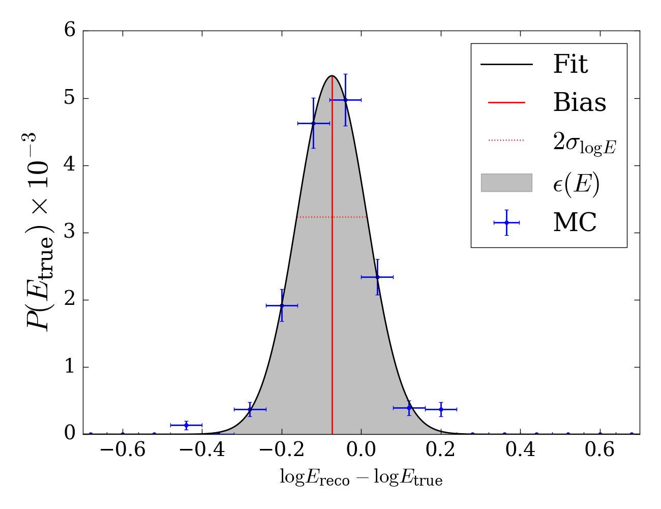
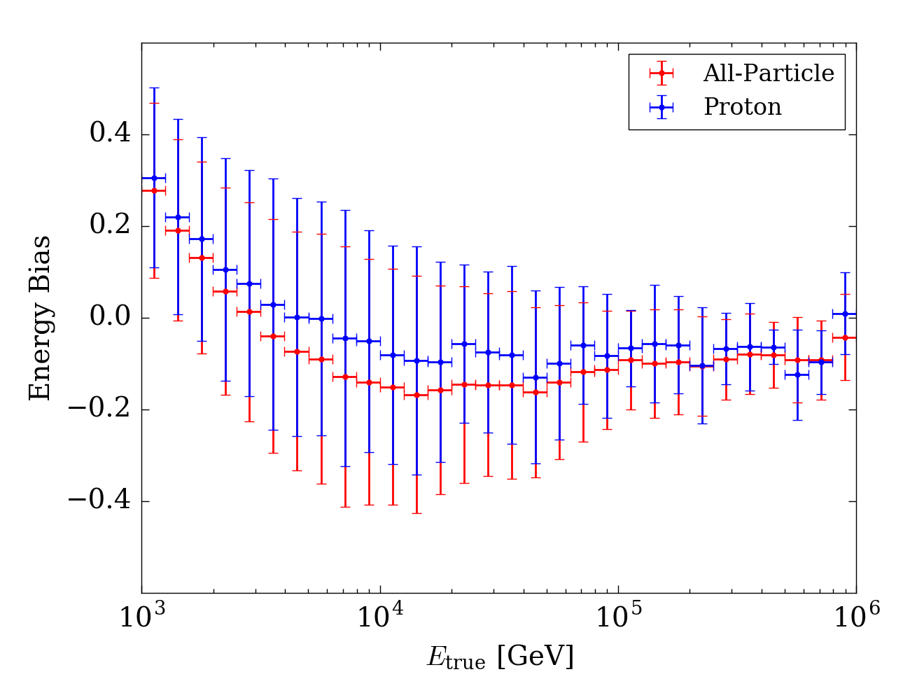
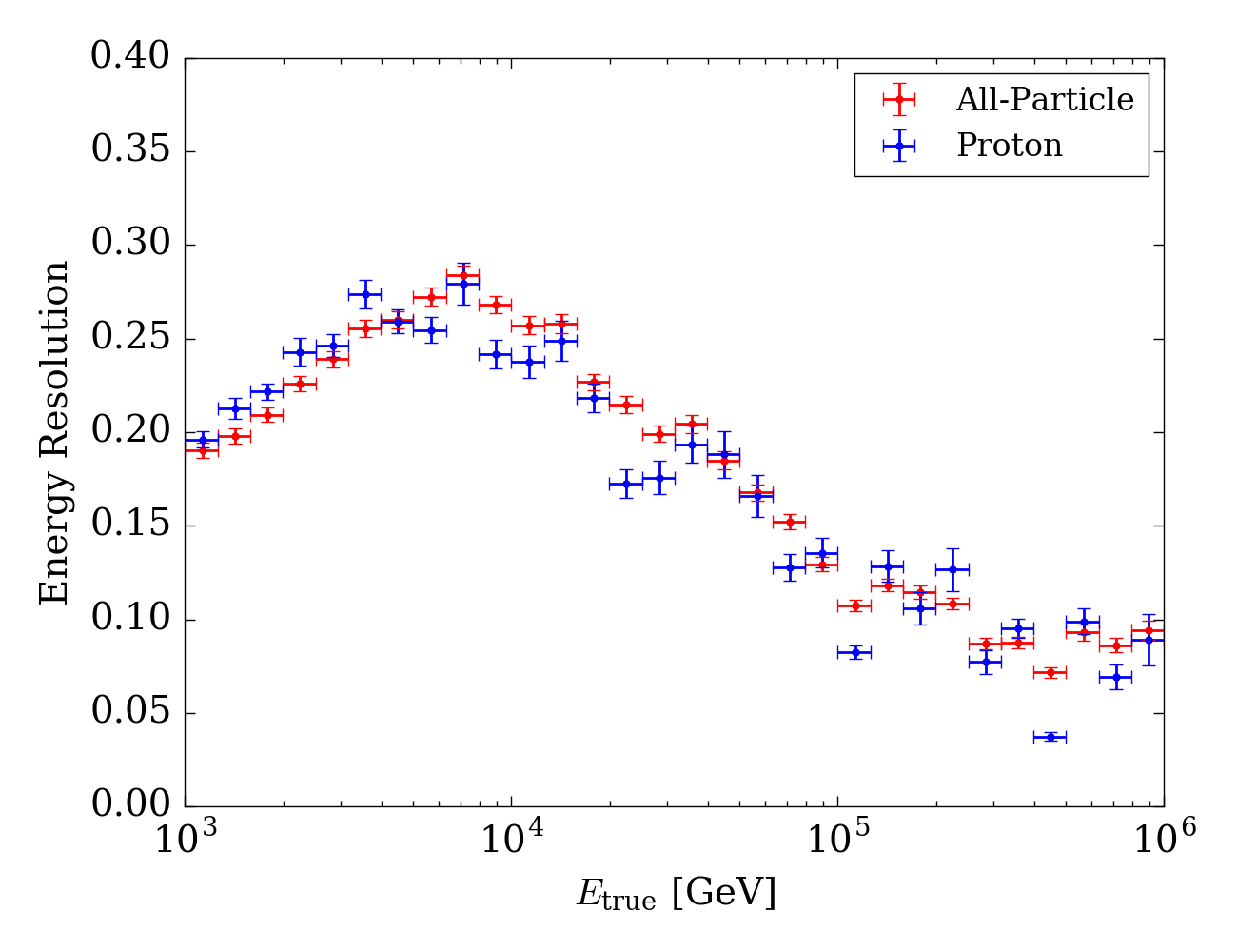
The resulting performance is evaluated via the bias distribution, defined by the difference between the logarithms of the reconstructed and true energy values, $\textnormal{bias}=\log{E_{\textnormal{reco}}}-\log{E_{\textnormal{true}}}$, shown for a single true energy bin in the leftmost panel of figure 1. The mean of this distribution defines the energy bias or offset and the width defines the energy resolution, which are shown as a function of energy in the remaining panels of figure 1, provided the event selection criteria for the most vertical zenith bin. We also identify the integral of the distribution as the efficiency $\epsilon$ to reconstruct events in that energy bin. Above 10 TeV, the bias is estimated to be less than an energy bin width, and the energy resolution is $<60\%$, improving with increasing energy.

3 The all-particle spectrum from vertical data

For the all-particle spectrum analysis, we select reconstructed air-showers within the first zenith bin of the energy estimation tables, $\theta<16.7^{\circ}$. In addition, we apply a set of selection cuts to reduce the uncertainty on the shower observables. In particular, we choose events that pass the arrival direction and core reconstruction procedures, have a minimum multiplicity threshold $N_{hit}\geq 75$ PMTs, and have activated at least $40$ PMTs within $40$ m of the shower core ($N_{r40}\geq 40$), the latter to ensure EAS with cores on or within $15\,\mbox{m}$ of the HAWC array. Provided the above selection criteria, the core resolution is estimated to be $10$ m at $10$ TeV, dropping below $8$ m above $100$ TeV, while the angular resolution is found to be $\sim 0.5^{\circ}$ above $10$ TeV.

(a)

(b)

Figure 2: The left panel shows the efficiencies $\epsilon(E_{\textnormal{true}})$ for all cosmic ray particles, and proton, helium, and iron components. The energy response matrix $P(E_{\textnormal{reco}}|E_{\textnormal{true}})$ for all species using the nominal composition model is shown on the right.

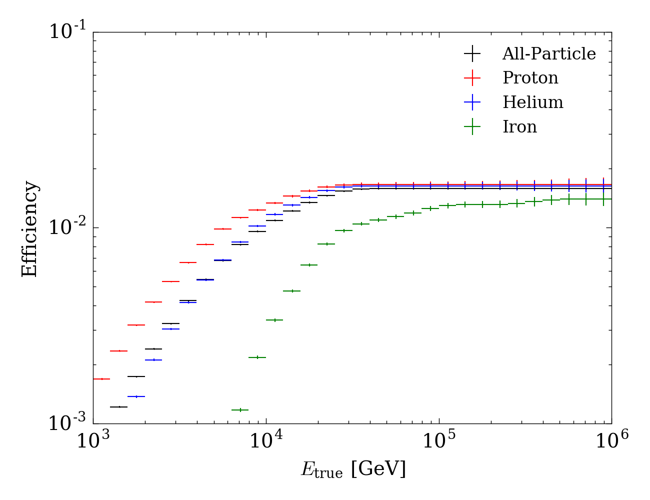
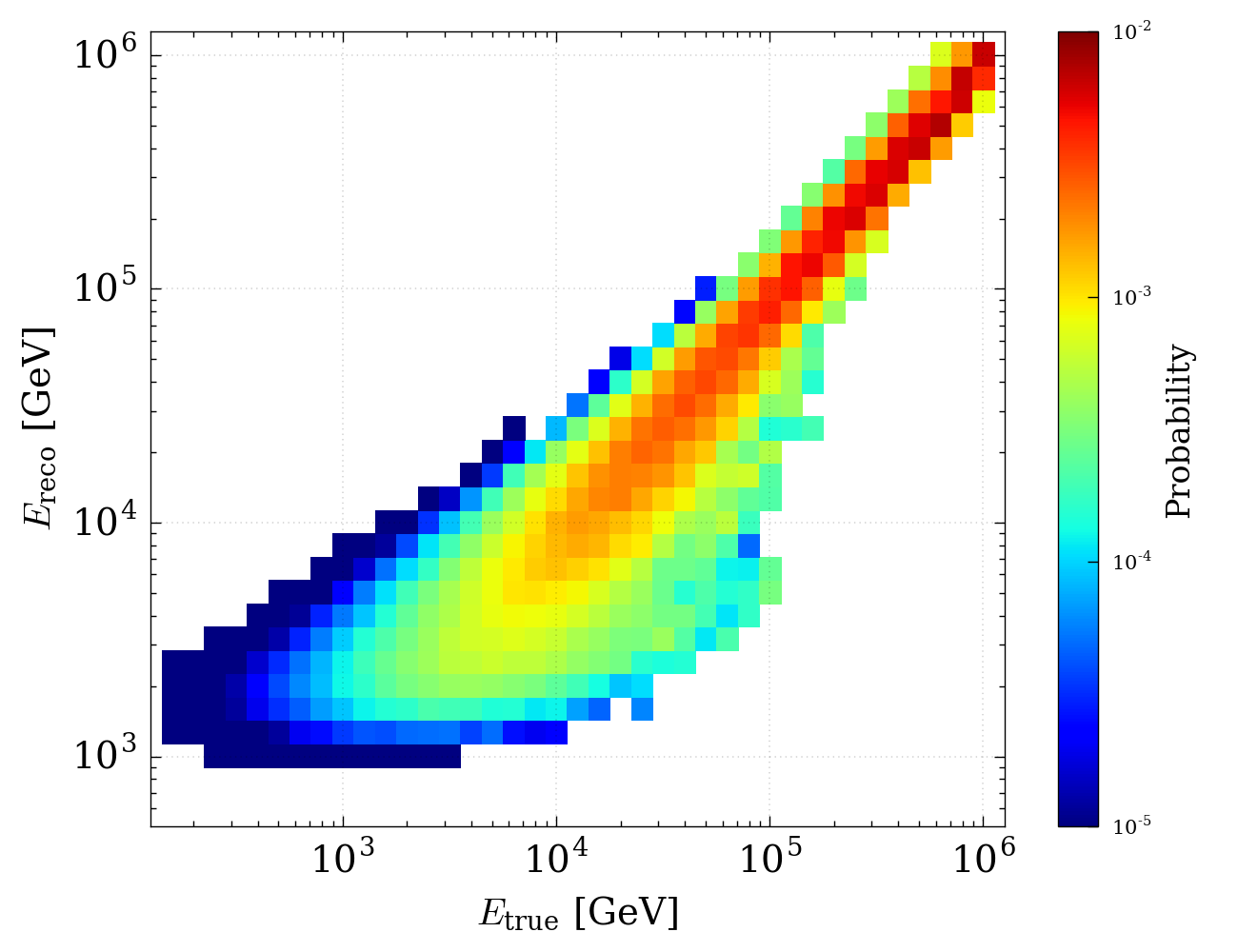
The smearing of the primary particle’s estimated energy including detector effects such as limited core and angular resolutions must be taken into account in order to measure the cosmic ray flux. This is summarized by the detector response matrix, as shown in figure 2 which is determined from simulation, including the assumed composition model and selection criteria. Following the iterative method presented in [13], the observed reconstructed energy distribution $N(E_{\textnormal{reco}})$ from data is to be unfolded with the energy response to obtain the measured all-particle energy distribution, $N(E_{\textnormal{true}})$. The analysis is performed iteratively: an initial estimate of $N(E_{\textnormal{true}})$ is convolved with the response matrix providing an improved estimate, which is used again until variations on $N(E_{\textnormal{true}})$ from one iteration to the next are negligible. The differential flux is then calculated from the final $N(E_{\textnormal{true}})$ according to the following:

$$\Phi(E)=\frac{N(E_{\textnormal{true}})}{\Delta t\Delta\Omega\ A_{throw}\ \Delta E}\,,$$ (2)

where $\Delta t$ is the observation time, $\Delta\Omega$ is the solid angle interval, $\Delta E$ is the energy bin width centered at $E_{\textnormal{true}}$, $A_{throw}$ is the simulated throwing area. The efficiency, $\epsilon(E_{\textnormal{true}})$, shown in figure 2 is taken into account in the unfolding procedure.

Figure 3: Left panel: $f_{hit}$ as a function of the reconstructed energy. The horizontal line at $f_{hit}=0.97$ represents the lower limit of the saturation region and the vertical line, the threshold energies where saturation effects begin. Curves were calculated using MC data and our nominal composition model. Right panel: Mean values of the expected age parameter for vertical EAS against the estimated shower energy for different primaries and for our nominal composition model (labelled as all). The HAWC data is also shown for comparison. Errors on the mean are shown. The segmented line represents the $s_{He-C}$ cut.

4 Spectrum of the light component of cosmic rays from vertical and inclined EAS

In order to estimate the spectrum of the light component of cosmic rays (H plus He nuclei), we select a subsample dominated by the primaries in which we are interested in. Then we construct its energy distribution, which we again correct for migration effects using an unfolding algorithm. Next, we correct the unfolded histogram for the abundance of heavy nuclei ($Z\geq 3$) and from the result, we reconstruct the corresponding energy spectrum of the light mass group of cosmic rays by correcting for the trigger, reconstruction, and selection efficiency of H and He primaries.

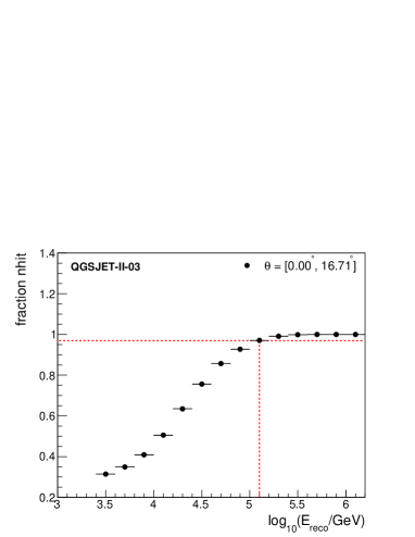
Before selecting the light subsample, first we apply a set of quality cuts on the data. In particular, we use similar selection cuts to those described in the previous section, but in order to further reduce the uncertainty in the core position, we employed $N_{r40}\geq 60$. In addition, we also remove low energy events ($E_{\textnormal{reco}}<10^{3.5}\,\mbox{GeV}$ ) from the low efficiency region using $f_{hit}\geq 0.3$, where $f_{hit}$ is the fraction of hit PMT’s at HAWC during the event [3]. These cuts were applied on both the data and the MC simulations. From the latter, we found that the mean core bias of EAS with $E_{\textnormal{reco}}=10^{4}-10^{5}\,\mbox{GeV}$ is smaller than $11\,\mbox{m}$, while the energy resolution is $\leq 42\%$. Here, $E_{\textnormal{reco}}$ is the reconstructed energy, which was estimated using the method described in section 2. We have restricted the analysis to energies $E_{\textnormal{reco}}\leq 10^{5}\,\mbox{GeV}$ as the number of hit PMT’s is saturated above this threshold energy. The latter can be seen in fig. 3, left, where $f_{hit}$ is shown as a function of $E_{\textnormal{reco}}$ for our nominal composition model and for EAS with $\theta<16.71^{\circ}$. As we can see on this plot, for vertical cosmic-ray showers, we are constrained to the TeV energy regime. This problem will be solved with the upgrade of HAWC [22]. Meanwhile, we are also investigating the possibility of using inclined EAS to study the high energy regime, since we have observed that the threshold energy for saturation increases with the zenith angle.

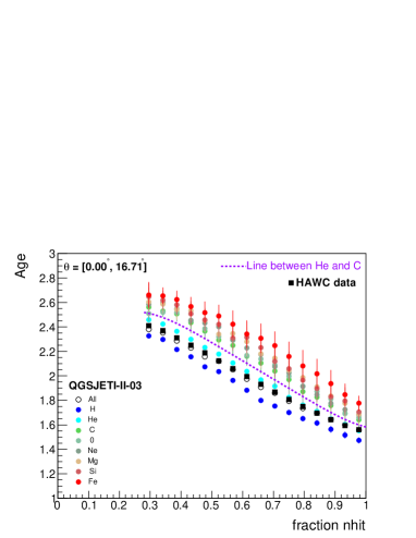
Now, in order to select our light subsample from the selected events, we make use of the age parameter, which is sensitive to the primary composition. This is illustrated, for example, in fig. 3, right, where the mean value of $s$ is presented as a function of $f_{hit}$, for different CR nuclei and vertical events. The plot was derived using MC data for different primaries and our nominal model. It shows that the age parameter increases with the mass of the primary nuclei and, in addition, decreases with $E_{\textnormal{reco}}$. This is understood from the fact that light primaries and high energy cosmic rays interact deeper in the atmosphere and hence produce EAS with steeper lateral distributions at ground level. To perform the selection, we apply a cut, $s_{He-C}$, located between the predicted curves for He and C (see fig. 3, right) on the data. If the events satisfy $s<s_{He-C}$, then they are classified into the light mass group of cosmic rays, otherwise they are considered as a part of the heavy component. In general, according to MC simulations, with our nominal composition model, the retention fraction of protons and helium nuclei in the light subsample is $\gtrsim 69$%, while its purity is $\gtrsim 84\%$ for vertical EAS with $E_{\textnormal{reco}}\geq 10^{3.5}\,\mbox{GeV}$.

For the mass group separation we have used the shower age, $s$ as a function of $f_{hit}$. However, we have found that the separation can be also carried out using $E_{\textnormal{reco}}$ instead of $f_{hit}$ with almost no changes in the final results. This is understood from the fact that $f_{hit}$ is proportional to $E_{\textnormal{reco}}$ below the saturation region (c.f. fig. 3, left) and because the energy dependence of $f_{hit}$ is not affected by the mass of the primary nuclei. One important point that should be stressed is that the dependence of $s$ on $f_{hit}$ for an individual element has little dependence on the spectral index, $\gamma$, of the corresponding energy spectrum. Using MC simulations, we found that a change $\Delta\gamma=\pm 0.2$ in the spectrum of the elemental groups leads to variations within $1\,\%$ in the corresponding $s(f_{hit})$ curves, which implies an independence of the $s_{He-C}$ cut from $\gamma$ and the composition model. However, it is expected a dependence on the hadronic interaction model, which will be investigated in a further study.

Figure 4: Left panel: The energy response matrix for the light subsample calculated from our nominal composition model. The vertical axis represent the reconstructed energy, and the horizontal axis, the true EAS energy. The color code indicates the probability $P^{\prime}(E_{\textnormal{reco}}|E_{\textnormal{true}})$, which just takes into account migration effects and does not considers neither trigger, reconstruction or selection efficiencies nor corrections from the expected fraction of heavy elements in the selected sample. Right panel: Effective areas used for the calculation of the spectra for the light mass group of cosmic rays. The curve was derived from MC simulations using our nominal composition model. At high energies $E_{\textnormal{true}}>10^{5.5}\,\mbox{GeV}$ a loss of efficiency is observed in the above effective area due to the saturation effect in $f_{hit}$.

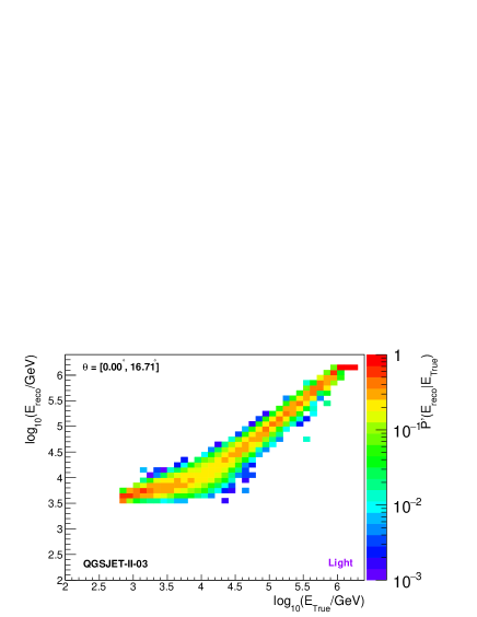
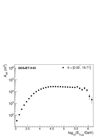
After selecting the light subsample, we then build the corresponding energy histogram and apply to it a Bayesian-inspired unfolding procedure [13] to correct for migration effects using a response matrix, $P^{\prime}(E_{\textnormal{reco}}|E_{\textnormal{true}})$, derived from MC simulations for our nominal composition model. Employing the above simulations, we also found some appropriate factors, $f_{corr}$, to be applied to the unfolded spectra to correct it for the expected fraction of heavy elements. These correction factors are defined as the inverse of the expected fraction of H and He primaries inside the corresponding energy bin. Finally, the energy spectra for the light component of cosmic rays is estimated by using formula 2. Here, $A_{throw}$ is replaced by the effective area, $A_{eff}$, which is defined as the product of $f_{corr}$ and the effective area for protons and helium nuclei in the subsample, $A_{eff}^{H+He}$, which is proportional to the efficiency $\epsilon^{H+He}$ for detecting an hydrogen/helium-induced EAS and classifying it as a part of our light subsample. Both, the response matrix and the effective area are presented in fig. 4. We should emphasize that the response matrix for the light sample is defined in such a way that

$$\sum_{j=1}P^{\prime}(E_{\textnormal{reco},j}|E_{\textnormal{true},i})=\frac{1}{f_{corr}(E_{\textnormal{true},i})\cdot\epsilon^{H+He}(E_{\textnormal{true},i})}\sum_{j=1}P(E_{\textnormal{reco},j}|E_{\textnormal{true},i})=1,$$ (3)

where $P(E_{\textnormal{reco}}|E_{\textnormal{true}})$ takes into account efficiency effects and it is corrected with $f_{corr}$ for the presence of heavy elements in the light subsample.

One of the main sources of systematic uncertainties in the procedure besides the influence of the hadronic interaction model is the composition dependence of the response matrix and the effective area. In order to evaluate the former, we have estimated both $P^{\prime}(E_{\textnormal{reco}}|E_{\textnormal{true}})$ and $A_{eff}$ using different models with distinct elemental abundances as predicted by the Polygonato model [15], and from fits to measurements from ATIC-2 [24], MUBEE [25] and JACEE [26].

We will apply the whole procedure above described to the experimental data soon. At the moment, we present in fig. 3, right, the $s(f_{hit})$ distribution of the selected data that we will use in the analysis, which consists of events collected during a complete HAWC run performed on June 2nd, 2016. We have employed this particular data set because the MC simulations use the detector configuration of this specific run. The selected showers were chosen as described at the beginning of this section but without using the age cut. The aforementioned data set contains about $2.3$ million events, while the data set with the light subsample contains $\sim 1.4$ million EAS. From fig. 3, right, we see that the measured distribution follows pretty well the predictions of the nominal composition model, which might indicate a dominance of the light component in the spectrum of cosmic rays in the energy interval $E_{\textnormal{reco}}=10^{4}-10^{5}\,\mbox{GeV}$. One of the next steps will be to study the robustness of both the method described in this section and the corresponding conclusions with the high-energy hadronic interaction model.

Acknowledgements

We acknowledge the support from: the US National Science Foundation (NSF); the US Department of Energy Office of High-Energy Physics; the Laboratory Directed Research and Development (LDRD) program of Los Alamos National Laboratory; Consejo Nacional de Ciencia y Tecnología (CONACyT), México (grants 271051, 232656, 260378, 179588, 239762, 254964, 271737, 258865, 243290, 132197), Laboratorio Nacional HAWC de rayos gamma; L’OREAL Fellowship for Women in Science 2014; Red HAWC, México; DGAPA-UNAM (grants IG100317, IN111315, IN111716-3, IA102715, 109916, IA102917); VIEP-BUAP; PIFI 2012, 2013, PROFOCIE 2014, 2015; the University of Wisconsin Alumni Research Foundation; the Institute of Geophysics, Planetary Physics, and Signatures at Los Alamos National Laboratory; Polish Science Centre grant DEC-2014/13/B/ST9/945; Coordinación de la Investigación Científica de la Universidad Michoacana. Thanks to Luciano Díaz and Eduardo Murrieta for technical support.

References

- [1] T. Stanev et al., Front. Phys. 8 (2013) 748; T. Stanev et al., NIMA 742 (2014) 42.
- [2] B. Bartoli et al., Phys. Rev. D 92 (2015) 092005.
- [3] A. U. Abeysekara et. al (HAWC Collab.), arXiv:astro-ph/1701.01778.
- [4] D. Heck et al., Report No. FZKA 6019, Forschungszentrum Karlsruhe-Wissenhaltliche Berichte (1998).
- [5] A. Ferrari, et al., CERN-2005-10 (2005), INFN/TC_05/11, SLAC-R-773; G. Battistoni et al., AIP Conference Proceedings 896 (2007) 31.
- [6] S. Ostapchenko, Phys. Rev. D 83 (2011) 014018.
- [7] S. Agostinelli et al., NIMA 506 (2003) 250.
- [8] M. Aguilar et al. (AMS Coll.), PRL 114(17) (2015) 131103; PRL 115(21) (2015) 211101.
- [9] H. S. Ahn et al. (CREAM Coll.), ApJ 707 (2009) 593; APJ 728(2) (2011) 122.
- [10] O. Adriani et al. (PAMELA Coll.), Science 332 (2011) 69.
- [11] K. Kamata and J. Nishimura, Prog. of Theor. Phys. Supp. 6 (1958) 93.
- [12] Kelly Malone , The gamma-ray sky above 50 TeV with the HAWC Observatory, April Meeting of the American Physical Society, January 2017.
- [13] G. D’Agostini, NIMA 362(2-3) (1995) 487.
- [14] T. K. Gaisser, Astrop. Phys. 35(12) (2012) 801.
- [15] J. R. Hörandel, Astrop. Phys. 19(2) (2003) 193.
- [16] T. Pierog and K. Werner, Nuclear Physics B - Proceedings Supplements 196 (2009) 102.
- [17] S. Fletcher, et al., Phys. Rev. D 50(9) (1994) 5710.
- [18] A. D. Panov et al. (ATIC Coll.), Bull. Russ. Acad. Sci. Phys. 73(5) (2009) 564.
- [19] H. Tanaka et al. (GRAPES-3 Coll.), J. of Phys. G Nuc. Phys. 39(2) (2012) 025201.
- [20] G. Di Sciasco et al., (ARGO-YBJ Coll.), Proc. of the Vulcano Workshop 2014, Vulcano, Italy, (2014).
- [21] M. Amenomori et al. (Tibet AS Coll.), Adv. Space Res. 42(3) (2008) 467.
- [22] V. Joshi et al. (HAWC Coll.), Proc. of the 35th ICRC, Busan, Korea (2017).
- [23] R. Gold, Report ANL-6984, Argonne, USA, 1964.
- [24] A. D. Panov et al., (ATIC-2 Collab.), Bull. Russ. Acad. Sci. Phys. 71 (2007) 494.
- [25] V.I. Zatsepin et al. (MUBEE Collab.), Proc. of the 23rd ICRC, editors: D.A. Leahy, R.B. Hickws, and D. Venkatesan, World Scientific, Vol. 2 (1993) 13.
- [26] Y. Takahashi et al. (JACEE Coll.), Nucl. Phys. B (Proc. Suppl.) 60B (1998) 83.