Asymmetric Thin-Shell Wormholes

Abstract

Spacetime wormholes in isotropic spacetimes are represented traditionally by embedding diagrams which were symmetric paraboloids. This mirror symmetry, however, can be broken by considering different sources on different sides of the throat. This gives rise to an asymmetric thin-shell wormhole, whose stability is studied here in the framework of the linear stability analysis. Having constructed a general formulation, using a variable equation of state and related junction conditions, the results are tested for some examples of diverse geometries such as the cosmic string, Schwarzschild, Reissner-Nordström and Minkowski spacetimes. Based on our chosen spacetimes as examples, our finding suggests that symmetry is an important factor to make a wormhole more stable. Furthermore, the parameter $\gamma$, which corresponds to the radius dependency of the pressure on the wormholes’s throat, can affect the stability in a great extent.

I Introduction

The history of wormholes goes back to the embedding diagrams of Ludwig Flamm Flamm in the newly discovered Schwarzschild metric in 1916. Later on, in 1935, Einstein and Rosen ER in search of a geometric model for elementary particles rediscovered a wormhole as a tunnel connecting two asymptotically flat spacetimes. The minimum radius of the tunnel, now known as the throat connecting two geometries, was interpreted as the radius of an elementary particle. The idea of wormhole did not go in much popularity until Morris and Thorne MT gave a detailed analysis and in certain sense initiated the modern age of wormholes as tunnels connecting two spacetimes. It was already stated by Morris and Thorne that the energy density of such an object, if it ever exists, must be negative; a notorious concept in the realm of classical physics. In quantum theory, however, rooms exist to manipulate and live along peacefully with negative energy densities. Being a classical theory, general relativity must find the remedy within its classical regime without resorting to any quantum. At this stage, an important contribution came from Visser, who found a way to confine the negative energy density zone to a very narrow band of spacetime known as the thin-shell MV1 . The idea of thin-shell wormholes (TSWs) became as popular and interesting as the standard wormholes, verified by the large literature in that context TSW . For some more recent works we refer to TSW2 . Let us also remark that there have been attempts to construct TSWs with total positive energy against the negative local energy density PE . This has been possible only by changing the geometrical structure of the throat, namely from spherical/circular to non-spherical/non-circular geometry, depending on the dimensionality. Stability of TSW is another important issue that deserves mentioning and investigation for the survival of a wormhole STABILITY .

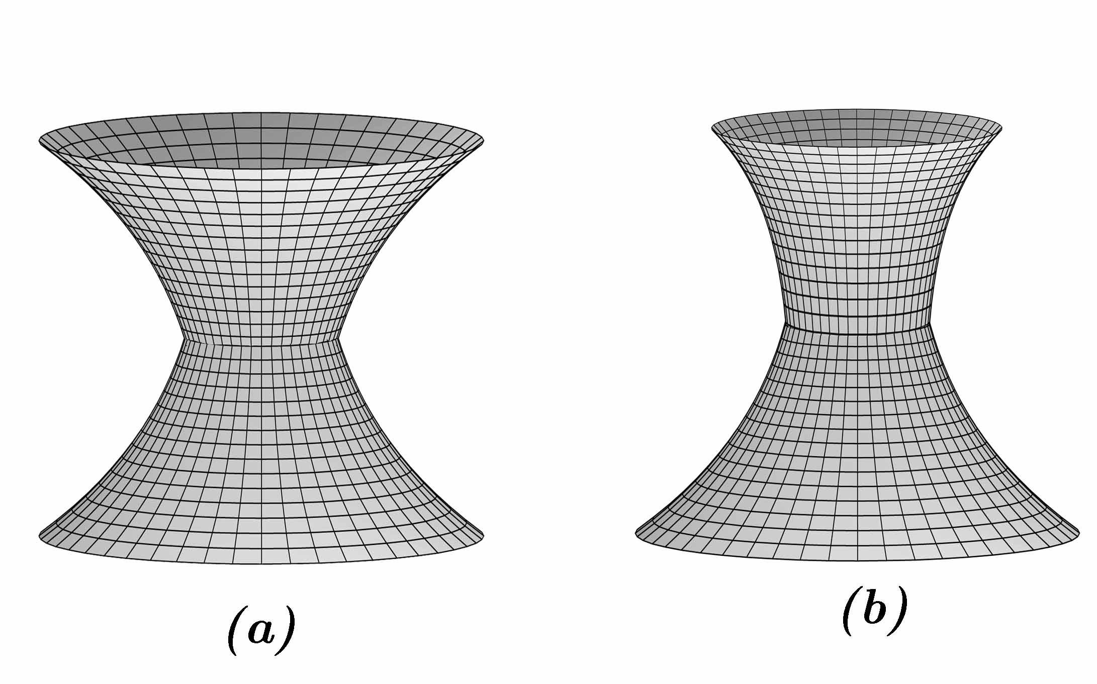
Figure 1: Schematic embedding diagram for a symmetric TSW (a) and an ATSW (b). The throat, on minimum radius hypersurface, separates two asymptotically flat spacetimes that are not the mirror images of each other. The upper and lower hyperboloids represent spacetimes with unequal matter content, joined at the throat in accordance with the junction conditions. Obviously, the slopes of tangent vectors to the hyperboloids at the throat are not continuous.

In this paper, we introduce TSWs, that are constructed from asymmetric spacetimes in the bulk ASYMMETRY . So far, the two spacetimes on different sides of the throat, are made from the same bulk material. Our intention is to consider different spacetimes, or at least different sources in common types of spacetimes in order to create a difference between the two sides. Naturally, the reflection symmetry about the throat in the upper and lower halves will be broken and in consequence new features are expected to arise which is the basic motivation for the present study. Note that for non-isotropic bulks, asymmetric TSWs emerge naturally. For example, we consider Reissner-Nordström (RN) spacetimes on both sides with different masses and charges in two sides of the throat; Or two cosmic string (CS) spacetimes with different deficit angles to be joined at the throat. This type of TSW, which we dub as asymmetric TSW (ATSW), has not been investigated so far. For this reason, we will be focusing on such wormholes. One may anticipate that the asymmetry of the wormhole will have an impact on particle geodesics, light lensing, and other matters. Asymmetry may act instrumental in the identification of TSWs in nature, if there exists such structures. Our next concern will be to study the stability of such ATSW and novelties that will give rise, if there are any at all. As in the previous studies, an equation of state (EoS) is introduced at the throat with pressure and density to be used as the surface energy-momentum tensor. Then, the Israel junction conditions Israel relate these variables within an energy equation (see Eq. 16), in which $V_{\text{eff}}\left(a\right)$ is an effective potential. Taking derivative of the energy equation (16) will naturally yield the equation of motion. Expansion of $V_{\text{eff}}\left(a\right)$ about an equilibrium radius of the throat, say $a=a_{0}$, demands the second derivative $V_{\text{eff}}^{\prime\prime}\ (a_{0})\equiv\left.\frac{d^{2}V_{\text{eff}}\ (a)}{da^{2}}\right|_{a=a_{0}}$ to be positive. We search for the stability regions of such ATSW and compare with the symmetric ones.

At this point, we would like to give some information about the stability analysis and EoS that we shall employ. We adopt a generalized EoS, known as the variable EoS, defined by $p=p(\sigma,a)$, where the pressure $p$ depends on both the energy density $\sigma$ and the radius of the shell. This will bring an extra term defined by $\gamma\equiv-\frac{\partial p}{\partial a}\neq 0$, as a new degree of freedom. By this choice, the position of the shell also will play a vital role in our stability analysis. Since the expansion of the effective potential about the equilibrium radius will involve the second derivative of the energy density, emergence of parameter $\gamma\neq 0$ in the radial perturbation of the throat will provide us an extra degree of freedom to achieve $V_{\text{eff}}^{\prime\prime}\ (a_{0})>0$.

Another useful parameter in our analysis will be $\beta^{2}\equiv-\frac{\partial p}{\partial\sigma}$, so that together with $\gamma$, we shall investigate the stability regions with $V_{\text{eff}}^{\prime\prime}\ (a_{0})>0$. In brief, almost all the detailed information about TSWs studied so far are also valid for our ATSWs so that we shall refrain from repeating those arguments. Instead, we shall concentrate on the differences that arise due to the lack of the mirror symmetry through the throat.

The organization of the paper goes as follows. In section $II$ we give a general description for TSWs introducing, in particular, the asymmetric ones. Cosmic string application of ATSW makes the subject matter for section $III$. In analogy, the Schwarzschild-Schwarzschild ATSW is considered for section $IV$. Section $V$ investigates the ATSW constructed from the Schwarzschild and Reissner-Nordström spacetimes. Our conclusion to the paper follows in section $VI$. Some mathematical details for the formalism are given in the Appendix.

II General Formulation

Having set the general forms of the metrics of the two spacetime geometries connected by the ATSW

$$ds_{i}=-f(r_{i})dt_{i}^{2}+\frac{1}{f(r_{i})}dr_{i}^{2}+r_{i}^{2}d\Omega_{i}^{2};\text{ }i=1,2,$$ (1)

we introduce the two spherically symmetric functions $f(r_{i})$ as follows;

$$f_{i}(r_{i})=k_{i}-\frac{2m_{i}}{r_{i}}+\frac{q_{i}^{2}}{r_{i}^{2}};\text{ }i=1,2,$$ (2)

where $k_{i}$ are two arbitrary constants expressing the cosmic constants of the two spacetimes, $m_{i}$ represent the masses and $q_{i}^{2}$ stand for the sum of the squares of the net electric and magnetic charges of the black holes in the two spacetimes as observed by a distant observer. Also, in Eq. (1), $d\Omega_{i}^{2}$ traditionally stands for $d\theta_{i}^{2}+\sin^{2}\theta_{i}d\phi_{i}^{2}$. In the case $\left|q_{i}\right|\leq m_{i}/\sqrt{k_{i}}$, the singularity is hidden behind an outer horizon denoted by

$$r_{+i}=\frac{1}{k_{i}}\left(m_{i}+\sqrt{m_{i}^{2}-k_{i}q_{i}^{2}}\right),$$ (3)

while for $\left|q_{i}\right|>m_{i}/\sqrt{k_{i}}$ the spacetime exhibits a naked singularity.

According to Visser MV1 , scissoring a region from each spacetime $\Sigma_{i}$ with $r_{i}\geq a$, where $a>r_{+i}$, and gluing them together at their common timelike hypersurface $\partial\Sigma_{i}=\left\{x|r_{i}-a=0,i=1,2\right\}$ results in a Riemannian, geodesically complete manifold marked by $\Sigma=\Sigma_{1}\cup\Sigma_{2}$. The hypersurface $\Sigma$ which represents a passage between the two spacetimes is a TSW and we will refer to $r=a$ as the throat of the wormhole. In order to examine the stability of the throat, one can spot a time-dependent throat, recognized by $r_{i}=a\left(\tau\right)$, or implicitly

$$\mathcal{F}_{i}(r_{i},\tau)=r_{i}-a\left(\tau\right)=0;i=1,2,$$ (4)

where $\tau$ is the proper time measured by the traveler on the shell.

In the context of Israel junction formalism Israel , two conditions must be satisfied at the wormhole’s throat, with the first one expecting a continuity in the first fundamental form and the second one requiring a discontinuity for the second fundamental form on the shell. Accordingly, the first condition gives rise to a unique metric on the shell given by

$$ds_{shell}^{2}=h_{ab}d\xi^{a}d\xi^{b}=-d\tau^{2}+a^{2}d\Omega^{2},$$ (5)

where now $\theta_{i}=\theta$ and $\phi_{i}=\phi$, while the second condition demands ($G=c=1$)

$$\left[K_{b}^{a}\right]-\delta_{b}^{a}\left[K\right]=-8\pi S_{b}^{a},$$ (6)

where $K_{b}^{a}$ and $K$ indicate the mixed extrinsic curvature tensor and the total curvature, respectively. Note that $S_{b}^{a}$ is the energy-momentum tensor of the shell and $\delta_{b}^{a}$ is the Kronecker delta. Furthermore, the square brackets signify a subtraction in the two sides’ curvatures, i.e.

$$\left[K_{b}^{a}\right]=K_{b1}^{a}-K_{b2}^{a},$$ (7)

with the convention that the indices $a$ and $b$ are those of the shell and take only $\tau$, $\theta$, and $\phi$. Having considered this, the next step should be the calculation of the extrinsic curvature for the two spacetime geometries. The standard definition of the extrinsic curvature for each side of the throat is given by (for simplicity, we remove the sub-index $i$)

$$K_{ab}=-n_{\mu}\left(\frac{\partial x^{\mu}}{\partial\xi^{a}\partial\xi^{b}}+\Gamma_{\alpha\beta}^{\mu}\frac{\partial x^{\alpha}}{\partial\xi^{a}}\frac{\partial x^{\beta}}{\partial\xi^{b}}\right),$$ (8)

where

$$n_{\mu}=\left(g^{\alpha\beta}\frac{\partial\mathcal{F}}{\partial x^{\alpha}}\frac{\partial\mathcal{F}}{\partial x^{\beta}}\right)^{-1/2}\frac{\partial\mathcal{F}}{\partial x^{\mu}}$$ (9)

is the spacelike four-normal vector satisfying $n_{\mu}n^{\mu}=+1$ for the timelike hypersurface, and $\Gamma_{\alpha\beta}^{\mu}$ are the Christoffel symbols of each bulk geometry. With some algebra, one calculates the mixed components of the extrinsic curvature tensor as

$$K_{bi}^{a}=diag\left(\frac{f_{i}^{\prime}+2\ddot{a}}{2\sqrt{f_{i}+\dot{a}^{2}}},\frac{\sqrt{f_{i}+\dot{a}^{2}}}{a},\frac{\sqrt{f_{i}+\dot{a}^{2}}}{a}\right),$$ (10)

where a prime $\left({}^{\prime}\right)$ stands for a total derivative with respect to the radial distance $r$, and an overdot $\dot{a}$ indicates a total derivative with respect to the proper time $\tau$. Combining Eqs. (6) and (10), together with the energy-momentum tensor of the shell chosen in the form

$$S_{b}^{a}=diag(-\sigma,p,p),$$ (11)

turns the second Israel junction conditions to the following set of equations;

$$\sigma=\frac{-1}{4\pi a}\left(\sqrt{f_{1}+\dot{a}^{2}}+\sqrt{f_{2}+\dot{a}^{2}}\right),$$ (12)

and

$$p=\frac{1}{8\pi}\left(\frac{f_{1}^{\prime}+2\ddot{a}}{2\sqrt{f_{1}+\dot{a}^{2}}}+\frac{f_{2}^{\prime}+2\ddot{a}}{2\sqrt{f_{2}+\dot{a}^{2}}}\right)-\frac{\sigma}{2}.$$ (13)

Herein, $\sigma$ is the surface energy density of the shell whereas $p$ is the angular pressure of the shell. Note that for the matter of symmetry between the curvature and energy-momentum tensors’ elements of $\theta$ and $\phi$, yields two independent equations instead of three.

By taking derivative of the energy density (12) with respect to the proper time, one can investigate that the energy conservation relation

$$\dot{\sigma}=-\frac{2}{a}\dot{a}\left(p+\sigma\right)$$ (14)

holds between $\sigma$ and $p$, which alternatively can be expressed as

$$\sigma^{\prime}=-\frac{2}{a}\left(p+\sigma\right).$$ (15)

As can be perceived from the latter equation, $p$ and $\sigma$ are not independent quantities and can be considered related to each other through an ”Equation of State”. Although the generic barotropic EoS, $p=p\left(\sigma\right)$, used to be popular in the context of the linearized stability analysis of wormholes, more recently the variable EoS, $p=p\left(\sigma,a\right)$ has been used by Varela Lobo ; Varela which will be used in our stability analysis too.

From here on, the method of stability analysis of the wormhole will be quite similar to that of Lobo . With some mathematical manipulations, Eq. (12) can be expressed by

$$\frac{1}{2}\dot{a}^{2}+V_{\text{eff}}\left(a\right)=0,$$ (16)

where one can Taylor expand the effective potential

$$V_{\text{eff}}\left(a\right)=\frac{1}{2}\left[\frac{f_{1}+f_{2}}{2}-\frac{\left(f_{1}-f_{2}\right)^{2}}{\left(8\pi a\sigma\right)^{2}}-\left(2\pi a\sigma\right)^{2}\right]$$ (17)

about a presumed equilibrium radius $a_{0}$ to obtain

$$V_{\text{eff}}\left(a\right)=V_{\text{eff}}\left(a_{0}\right)+V_{\text{eff}}^{\prime}\left(a_{0}\right)\left(a-a_{0}\right)+\\ \frac{1}{2}V_{\text{eff}}^{\prime\prime}\left(a_{0}\right)\left(a-a_{0}\right)^{2}+O^{3}(a-a_{0}).$$ (18)

Evidently, the first two terms on the right-hand side of this expansion become zero; the first as a consequence of Eq. (17) and the second, $a_{0}$ represents an equilibrium radius. This implies

$$V_{\text{eff}}\left(a\right)\simeq\frac{1}{2}V_{\text{eff}}^{\prime\prime}\left(a_{0}\right)\left(a-a_{0}\right)^{2}$$ (19)

where $V_{\text{eff}}^{\prime\prime}\left(a_{0}\right)$ can be calculated through calculating consecutive derivations of Eq. (17) and substituting for $\sigma(a_{0})$ and $\sigma^{\prime}(a_{0})$ from Eqs. (12) and (15). However, one must assure that the derivation process is taken carefully since a second derivative of $\sigma$ arises in $V_{\text{eff}}^{\prime\prime}\left(a_{0}\right)$ due to the variable EoS. Mathematically speaking, this amounts to

$$\sigma^{\prime\prime}=\frac{2}{a}\left[\frac{3}{a}\left(p+\sigma\right)-p^{\prime}\right].$$ (20)

In the most general case, when the variable EoS $p=p\left(\sigma,a\right)$ is taken into account, we have

$$p^{\prime}=\sigma^{\prime}\frac{\partial p}{\partial\sigma}+\frac{\partial p}{\partial a},$$ (21)

and

$$\sigma^{\prime\prime}\left(a_{0}\right)=\left.\frac{2}{a^{2}}\left[\left(p+\sigma\right)\left(3+2\frac{\partial p}{\partial\sigma}\right)-a\frac{\partial p}{\partial a}\right]\right|_{a=a_{0}}.$$ (22)

From Eq. (19), we are interested in the cases where $V_{\text{eff}}^{\prime\prime}\left(a_{0}\right)>0$; these are the stable equilibrium states. Having collected Eq. (2) for the radially symmetric functions $f_{1}$ and $f_{2}$, together with Eqs. (12), (15) and (20)  for $\sigma$ and its derivatives,$\ V_{\text{eff}}^{\prime\prime}\left(a_{0}\right)$ can explicitly be acquired as

$$V_{\text{eff}}^{\prime\prime}\left(a_{0}\right)=-8\pi\left\{\left(4\beta^{2}+3\right)\sigma_{0}^{2}+2\left(\gamma a_{0}+2p_{0}\beta^{2}+3p_{0}\right)\sigma_{0}+4p_{0}^{2}\right\}+\frac{\Delta^{\prime\prime}}{2}+\\ \frac{\left[\left(4\beta^{2}-1\right)\sigma_{0}^{2}+\left(\left(4\beta^{2}-10\right)p_{0}+2a_{0}\gamma\right)\sigma_{0}-12p_{0}^{2}\right]\delta-2a_{0}\sigma_{0}\left(\sigma_{0}+2p_{0}\right)\delta^{\prime}-\frac{1}{2}a_{0}^{2}\sigma_{0}^{2}\delta^{\prime\prime}}{32\pi^{2}a_{0}^{4}\sigma_{0}^{4}}$$ (23)

in which for simplicity we introduced $\delta=\left(f_{20}-f_{10}\right)^{2}$ and $\Delta=\left(f_{10}+f_{20}\right).$ Here $f_{i0}$, $\sigma_{0}$ and $p_{0}$ are the appropriate values for $f_{i}$, $\sigma$ and $p$ at $a_{0}$ given by

$$f_{i0}=k_{i}-\frac{2m_{i}}{a_{0}}+\frac{q_{i}^{2}}{a_{0}^{2}};i=1,2,$$ (24)

$$\sigma_{0}=\frac{-1}{4\pi a_{0}}\left(\sqrt{f_{10}}+\sqrt{f_{20}}\right),$$ (25)

and

$$p_{0}=\frac{1}{8\pi}\left(\frac{f_{10}^{\prime}}{2\sqrt{f_{10}}}+\frac{f_{20}^{\prime}}{2\sqrt{f_{20}}}\right)-\frac{\sigma_{0}}{2},$$ (26)

respectively. Also, $\beta^{2}$ and $\gamma$ are introduced as the partial derivatives of $p$ with respect to $\sigma$ and $-a$, correspondingly;

$$\beta^{2}\equiv\frac{\partial p}{\partial\sigma},$$ (27)

and

$$\gamma\equiv-\frac{\partial p}{\partial a},$$ (28)

in which $\beta^{2},\gamma\in\mathbb{R}$.

Hereafter, the potential (23) will be employed in order to analyze the stability of an ATSW at its throat. During the last 30 years, this has been done by different authors for diverse spacetimes connected by a symmetric TSW. For example, a Schwarzschild-Schwarzschild (S-S) wormhole was studied in MV1 which in the framework of the present article can be evoked by setting

$$\left\{\begin{array}[]{c}k_{i}=1\\ m_{i}=M\\ q_{i}=0\\ \gamma=0\end{array}\right..$$ (29)

Similarly, the results for $V_{\text{eff}}^{\prime\prime}\left(a_{0}\right)$ of an RN-RN wormhole, as the one that has been analyzed in RNRN , are immediate by setting

$$\left\{\begin{array}[]{c}k_{i}=1\\ m_{i}=M\\ q_{i}=Q\\ \gamma=0\end{array}\right..$$ (30)

Let us comment that in the stability analysis of thin-shells (not TSWs), the spacetime geometries of the two sides of the thin-shell are different. Actually, this is how a physical thin-shell can be defined; roughly speaking, something whose two sides can be distinguished. Otherwise, our thin-shell will be merely an imaginary shell in the spacetime.

Now, one may ask the question can we have a TSW connecting two different geometries? As long as the existing horizons on the two sides (of both spacetimes) remain behind radius $a$, the answer is yes. As for this, we would like to have a thorough look at the more exciting cases of non-identical universes connecting wormholes. In the following, three cases are studied in detail: An ATSW with two Cosmic String geometries of different deficit angles are brought together (CS-CS* ATSW); an ATSW connecting two Schwarzschild universes of different central masses (S-S* ATSW); and finally an ATSW which provides a bridge between a Schwarzschild and a Reissner-Nordström universe (S-RN ATSW).

III A CS-CS TSW with Different Deficit Angles

The two CS universes are characterized by

$$\left\{\begin{array}[]{c}k_{1}=k\\ k_{2}=\left(1+\eta\right)k\\ m_{i}=0\\ q_{i}=0\end{array}\right.,$$ (31)

where $k$ and $\eta$ are two constants; $k>0$ and $\eta>-1$. Accordingly, equation (23) for $V_{\text{eff}}^{\prime\prime}\left(a_{0}\right)$ simplifies to

$$V_{\text{eff}}^{\prime\prime}\left(x_{0}\right)=\frac{-4\left(\beta^{2}+\frac{1}{2}\right)\sqrt{1+\eta}}{x_{0}^{2}}+\\ 4\pi\gamma\sqrt{k}\left[1+\sqrt{1+\eta}-\frac{\eta^{2}}{\left(1+\sqrt{1+\eta}\right)^{3}}\right],$$ (32)

where $x_{0}=\frac{a_{0}}{\sqrt{k}}$ is the reduced equilibrium radius. As can be seen easily, in case of a generic barotropic EoS $\left(\gamma=0\right)$, $V_{\text{eff}}^{\prime\prime}\left(a_{0}\right)$ in Eq. (32) immediately becomes zero for $\beta^{2}=-\frac{1}{2}$, which surprisingly depends neither on $x_{0}$ nor $\eta$. Notice that this rather general case reduces to a Minkowski-CS (M-CS) ATSW for $k=1$ when $\eta\neq 0$, and for $k=1$ when $\eta=0$ simplifies to a Minkowski-Minkowski (M-M) TSW, whereas still, the conclusion brought after Eq. (32) holds. On the other hand, in a more general perspective including a variable EoS, one obtains $\beta^{2}$ by solving $V_{\text{eff}}^{\prime\prime}\left(x_{0}\right)=0$, which leads to

$$\beta^{2}=\frac{4\pi x_{0}^{2}\sqrt{k}\gamma}{\sqrt{1+\eta}+1}-\frac{1}{2}.$$ (33)

Due to the restrictions on $k$ and $\eta$, the coefficient of $\gamma$ in Eq. (33) is obviously positive definite. This emphasizes that for negative values of $\gamma$, the stability region always shrinks. Conversely, any positive value for $\gamma$ results in a stronger stability, meaning that now there are more values available for $\beta^{2}$ to occupy in order to have a positive $V_{\text{eff}}^{\prime\prime}$. Nevertheless, at equilibrium, a positive value for $\gamma$ determines a negative value for $\frac{\partial p}{\partial a}$ by definition, which physically means that the pressure on the shell alters negatively with a change in radius. Hence, if presumably, the pressure is not negative itself, one may come up with the idea that the minus sign has emerged during the process of derivation. This in turn shows that for example in the case where $\gamma$ is proportional to a powered term, i.e. $x_{0}^{n}$, the power $n$ must be negative. Moreover, for certain values of $k$ and $\eta$, the coefficient of $\gamma$ behaves quadratically with respect to the reduced equilibrium radius $x_{0}$, indicating that for a general form of $\gamma\propto x_{0}^{n}$ the universal shape of $\beta^{2}$ against $x_{0}$ is predictable.

For the sake of comparison, the associated functions for $\beta^{2}$ are brought in the following for three arbitrary choices of $\gamma$ at equilibrium. Herein, coefficients are chosen such that they simplify the form of $\beta^{2}$ to the best for further analysis. Having considered this, we select

$$\gamma_{a}=\frac{-1}{4\pi\sqrt{k}}\Rightarrow\beta^{2}=-\frac{\left(\sqrt{1+\eta}-1\right)}{\eta}x_{0}^{2}-\frac{1}{2},$$ (34)

$$\gamma_{b}=\frac{-1}{4\pi\sqrt{k}x_{0}}\Rightarrow\beta^{2}=-\frac{\left(\sqrt{1+\eta}-1\right)}{\eta}x_{0}-\frac{1}{2},$$ (35)

and

$$\gamma_{c}=\frac{1}{4\pi\sqrt{k}x_{0}^{2}}\Rightarrow\beta^{2}=\frac{\left(\sqrt{1+\eta}-1\right)}{\eta}-\frac{1}{2}.$$ (36)

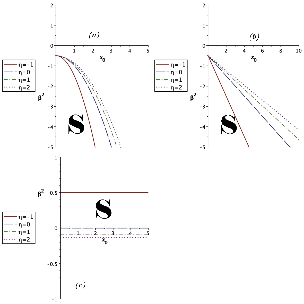
Figure 2: $\beta^{2}$ versus $x_{0}$ is plotted for a CS-CS* ATSW where $\gamma$ is selected as $a)$ $\gamma_{a}=1/4\pi\sqrt{k}$, $b)$ $\gamma_{b}=1/4\pi\sqrt{k}x_{0}$, and $c)$ $\gamma_{c}=1/4\pi\sqrt{k}x_{0}^{2}$. Each figure is drawn for four values of $\eta$. Note that $\eta=0$ is associated with an M-M TSW. Also, note that $\eta$ cannot adopt $-1$ and the corresponding graphs for $\eta=-1$ are brought as limits. A sign S implies the stable region.

Fig. 2 reflects the graphs for $\beta^{2}$ against $x_{0}$ for the three cases considered above. These figures show different features of stability in the vicinity of $a_{0}$ and beyond. The most important aspect is that there is always a range of values for $\beta^{2}$ for which the throat is stable, apart from any permitted values of $k$ and $\eta$. As another important outcome, although for $\gamma_{a}$ and $\gamma_{b}$ in Eqs. (34) and (35) $\beta^{2}$ is permanently negative in stable states, $\gamma_{c}$ in Eq. (36) makes it possible for $\beta^{2}$ to adopt positive values when $-1<\eta<0$. This is illustrated in Fig. 3.

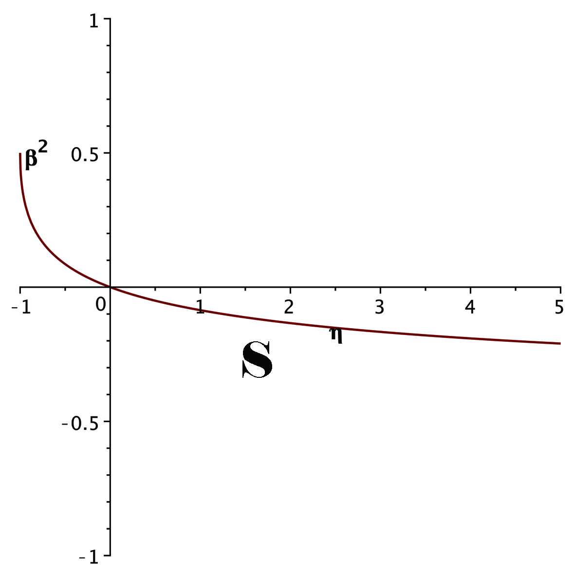
Figure 3: The plot of $\beta^{2}$ against $\eta$ for a CS-CS ATSW, when $\gamma=\gamma_{c}=1/4\pi\sqrt{k}x_{0}^{2}$. The figure implies that for domain $-1<\eta<0$, $\beta^{2}$ can be positive. A sign S implies the stable region.

A slightly different discussion is applied when again a variable EoS is on the agenda. Solving $V_{\text{eff}}^{\prime\prime}\left(a_{0}\right)=0$ for $\gamma$ leads to

$$\gamma=\frac{\left(\beta^{2}+\frac{1}{2}\right)\left(\sqrt{1+\eta}+1\right)}{4\pi\sqrt{k}x_{0}^{2}},$$ (37)

which can be rewritten by introducing

$$\gamma^{\ast}=\frac{4\pi\sqrt{k}\gamma}{\left(\beta^{2}+\frac{1}{2}\right)}$$ (38)

in the fashion

$$\gamma^{\ast}=\frac{\sqrt{1+\eta}+1}{x_{0}^{2}}.$$ (39)

The associated graph indicates that at equilibrium radius, for fixed values of $k$ and $\beta^{2}$, $\gamma$ ascends by an increase in $\eta$. The visualization of $\gamma^{\ast}$ against $x_{0}$ is brought in Fig. 4a for four values of $\eta$ ($\eta=-1$ is brought as a limit). Besides, equation (33) for $\gamma$ exhibits a particular feature that is, for $\beta^{2}=-\frac{1}{2}$, $\gamma$ vanishes identically. Also, $\gamma^{\ast}=2$ when $\eta$ is zero; for the case of two Cosmic String (CS) universes with the same deficit angle. Also, in Fig. 4b the behavior of $\gamma^{\ast}$ for a constant $x_{0}$ against parameter $\eta$ is projected.

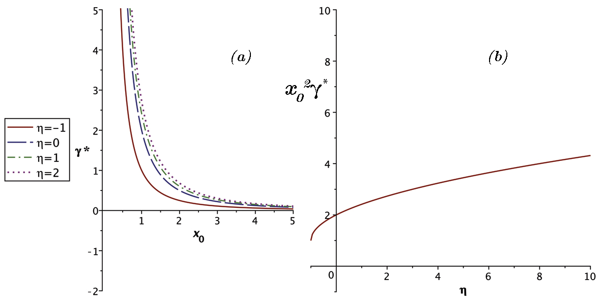
Figure 4: For a CS-CS* ATSW in case a variable EoS where $\beta^{2}\neq-1/2$, $a)$ shows $\gamma^{\ast}$ plotted against $x_{0}$ for four different values of $\eta$ ($\eta=-1$ is an inaccessible limit), and $b)$ shows $\gamma^{\ast}x_{0}^{2}$ plotted against $\eta$. A sign S implies the stable region.

IV An S-S TSW with Different Central Masses

As the next example, we look at the case in which the throat provides a transition between two Schwarzschild geometries possessing different central masses. In other words, we require

$$\left\{\begin{array}[]{c}k_{i}=1\\ m_{1}=M\\ m_{2}=(1+\epsilon)M\\ q_{i}=0\end{array}\right.,$$ (40)

for the two sides’ spacetimes, where $\epsilon$ is a constant; $\epsilon\geq-1$. Rewriting $V_{\text{eff}}^{\prime\prime}\left(a_{0}\right)$ from Eq. (23), it can be solved to obtain $\beta^{2}$ in terms of $\epsilon$, $\gamma$ and $x_{0}$, where $x_{0}\equiv\frac{a_{0}}{M}$ is the reduced radius (For the curious reader, the explicit forms of $V_{\text{eff}}^{\prime\prime}\left(a_{0}\right)$ and $\beta^{2}$ are brought in Appendix A). In the case of a barotropic EoS $\left(\gamma=0\right)$, one can plot $\beta^{2}$ against $x_{0}$ for various values of $\epsilon$. It is not hard to see from Eq. (40) that for the special case of $\epsilon=0$, the symmetric S-S wormhole studied by Poisson and Visser in TSW revives; the throat connects two Schwarzschild geometries with the same central masses. Furthermore, it is worth mentioning that for $\epsilon=-1$ the wormhole couples a Schwarzschild spacetime with a flat Minkowski spacetime. In Fig. 5, the graphs for $\beta^{2}$ against $x_{0}$ are depicted for different values of $\epsilon$; $\epsilon=-1.0,-0.5,0.0,0.5,$ and $1.0$. For $\epsilon=0.0$, the shaded areas are the regions of stability for the wormhole where $V_{\text{eff}}^{\prime\prime}$ is evidently positive. For other values of $\epsilon$ the stable regions are the same as $\epsilon=0.0$. However, in order to keep the figure less complicated we did not color those areas. For $\beta^{2}>0,$ Fig. 5 shows clearly that deviation from the symmetric TSW with $\epsilon\neq 0.0$ makes the region of stability smaller. This is the evidence that at least for the physical meaningful values of $\beta^{2},$ the more symmetric TSW is, the more stable it becomes against a radial linear perturbation.

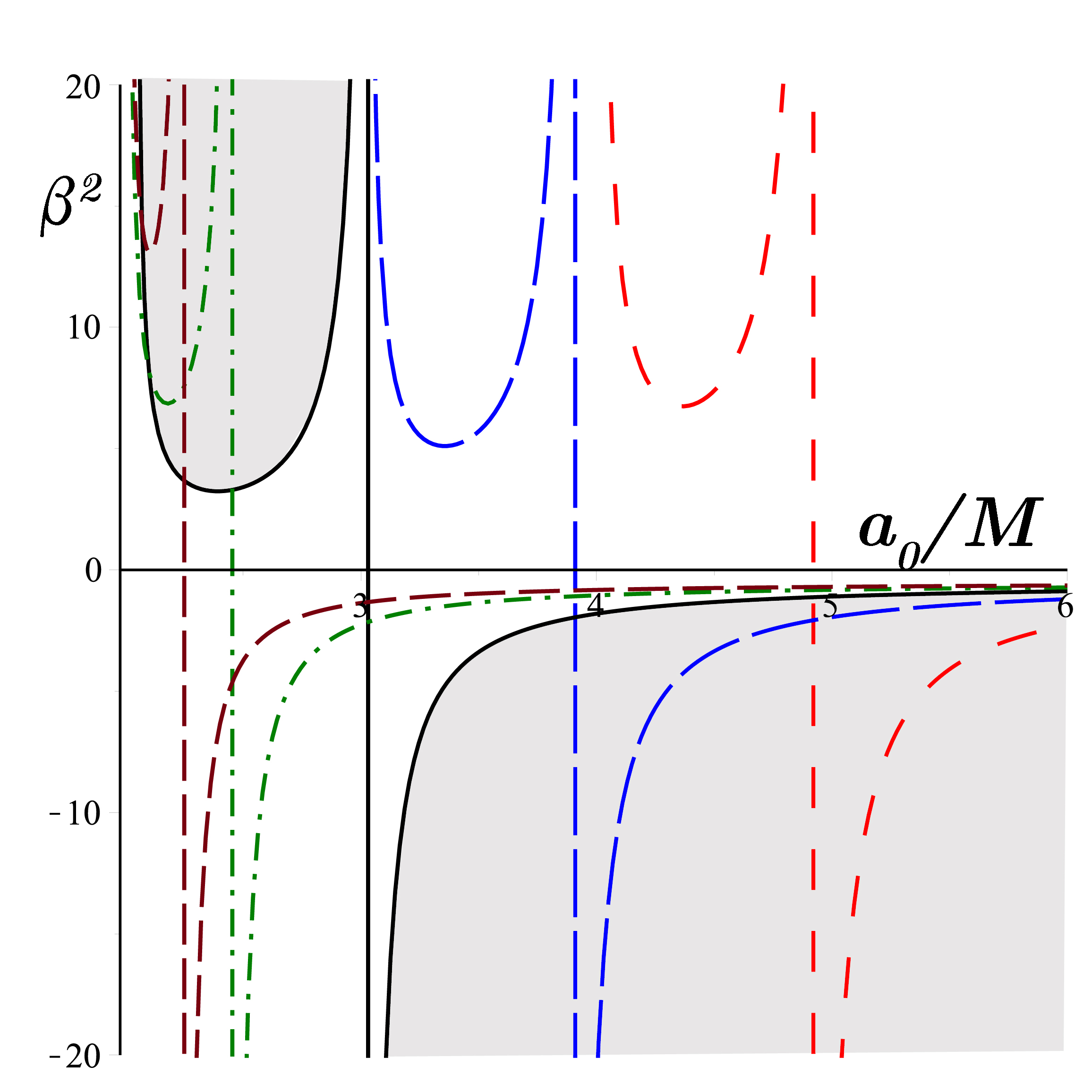
Figure 5: The plots of $\beta^{2}$ versus $x_{0}=\frac{a_{0}}{M}$ for an S-S* ATSW with $\gamma=0$ and (from left to right i.e., Brown-Dash, Green-Dash dot, Black-Solid, Blue-Long dash and Red-Space dash) $\epsilon=-1.0,-0.5,0.0,0.5$ and $1.0.$ The stable regions for $\epsilon=0.0$ are shaded. For the other values of $\epsilon$ the stable regions are the same as $\epsilon=0.0$ but are not coloured.

As another important example, let us consider the more general EoS $p=p\left(\sigma,a\right)$. Now, $\beta^{2}$ obtained by setting $V_{\text{eff}}^{\prime\prime}\left(a_{0}\right)$ equal to zero will have terms which include $\gamma$. If one brings these terms together, it can be apperceived that with a positive slope, $\beta^{2}$ is linear to $\gamma$. This implies that the arguments already represented in the previous section for a CS-CS* ATSW where a variable EoS was discussed, can be summoned here. Correspondingly, as a general statement concluded from the generic form of $\beta^{2}$ (brought in the Appendix), any negative value given for $\gamma$ results in an instability in the throat while any positive value for $\gamma$ stabilizes ATSW at its equilibrium radius. This is due to the fact that the coefficient of $\gamma$ in Eq. (A.2) is positive definite. Likewise, for the general form of $\gamma\propto$ $a^{n}$, if $n>0$/$n<0$, the growth/decay in stability/instability happens faster with $n$.

Let us now choose now a function for $\gamma$ such that it is proportional to $a^{-2}$, that is

$$\gamma=\frac{-1}{\pi M^{2}x_{0}^{2}}$$ (41)

merely for the sake of simplification. With the latter choice for $\gamma$, the behavior of $\beta^{2}$ versus $x_{0}$ is plotted in Fig. 6 for the same values of $\epsilon$. We observe that the zoomed-out gesture of the graphs has altered little from what we had seen in Fig. 5. This is due to the chosen values of the numerical quantities.

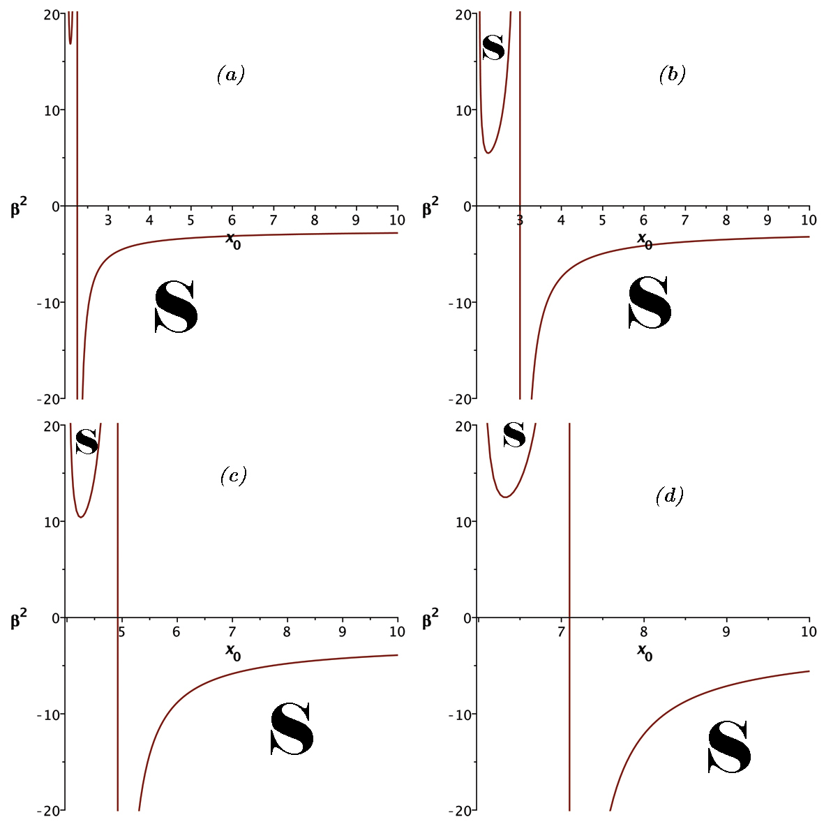
Figure 6: The plots of $\beta^{2}$ versus $x_{0}$ are given for an S-S* ATSW when $\gamma=-1/\pi M^{2}x_{0}^{2}$ while $a)$ $\epsilon=-1$, $b)$ $\epsilon=0$, $c)$ $\epsilon=1$, and $d)$ $\epsilon=2$. Although the generic shape of the plots has shown no drastic change compared with the case of a barotropic EoS, the shifts in the range of $\beta^{2}$ somehow state that the stability has decreased. A sign S implies the stable region.

On the other hand, things would change significantly if instead of Eq. (41) we were to pick

$$\gamma=\frac{1}{\pi M^{2}x_{0}^{2}}.$$ (42)

The associated plots for $\epsilon=-1,0,1,2$ are given in Fig. 7, where the dramatic changes in the regions of stability can be observed. The most important notion here is that now, for any radial distance, there are always positive values that $\beta^{2}$ could adopt.

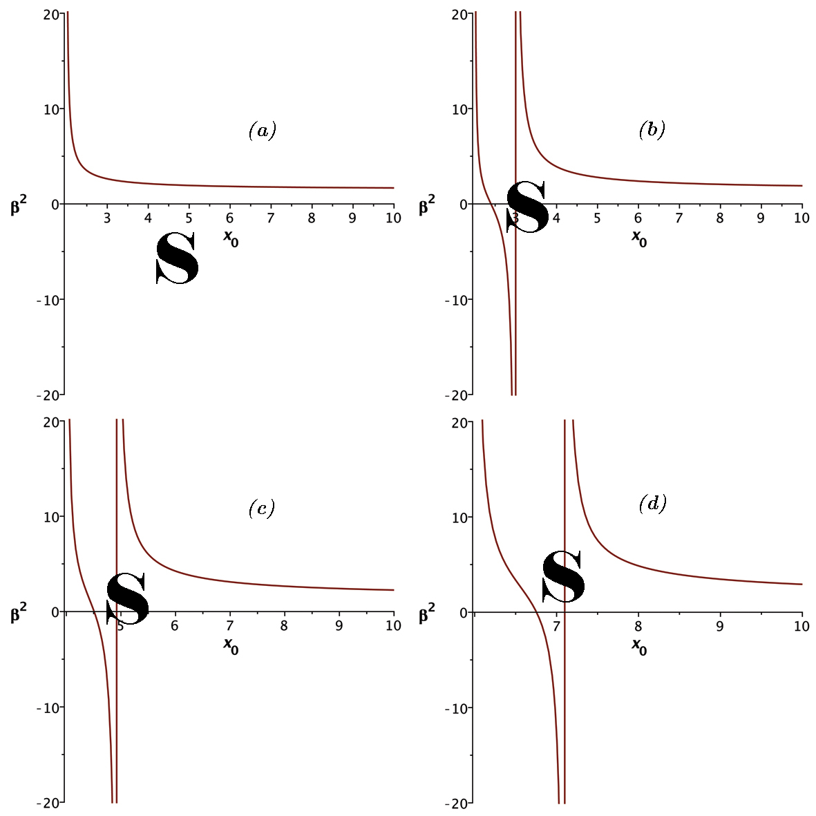
Figure 7: The plots of $\beta^{2}$ versus $x_{0}$ are given for an S–S* ATSW when $\gamma=1/\pi M^{2}x_{0}^{2}$ while $a)$ $\epsilon=-1$, $b)$ $\epsilon=0$, $c)$ $\epsilon=1$, and $d)$ $\epsilon=2$. Both the general shape and the ranges of the plot exhibit notable alterations with respect to the case of a barotropic EoS. A sign S implies the stable region.

As another result deduced from Figs. 5-7, although with an increase in $\epsilon$ the areas of stable regions constantly decrease, the region where $\beta^{2}$ can possess a positive value increases. The sign of $\beta^{2}$ is important on account of the association of $\beta$ with the speed of sound in the material existed on the thin shell; hence a positive value for $\beta^{2}$ somehow makes more sense, in physical terms.

As the last example for this section, let us have a look at a rather strange case where pressure is a function of the radius but not $\sigma$. This implies that $\beta^{2}=0$. Therefore, solving $V_{\text{eff}}^{\prime\prime}=0$ for $\gamma$ and redefining it as

$$\gamma^{\ast\ast}=8\pi M^{2}\gamma,$$

we arrive at an expression in terms of $x_{0}$ and $\epsilon$ i.e.

$$\gamma^{\ast\ast}=\frac{\left[x_{0}^{2}-3x_{0}\left(1+\epsilon\right)+3\left(1+\epsilon\right)^{2}\right]\left(x_{0}-2\right)^{2}\sqrt{\frac{x_{0}-2\left(1+\epsilon\right)}{x_{0}}}+\left[x_{0}-2\left(1+\epsilon\right)\right]^{2}\left(x_{0}^{2}-3x_{0}+3\right)\sqrt{\frac{x_{0}-2}{x_{0}}}}{x_{0}^{2}\left(x_{0}-2\right)^{2}\left[x_{0}-2\left(1+\epsilon\right)\right]^{2}}.$$ (43)

The associated graphs for four values of $\epsilon$ are plotted in Fig. 8.

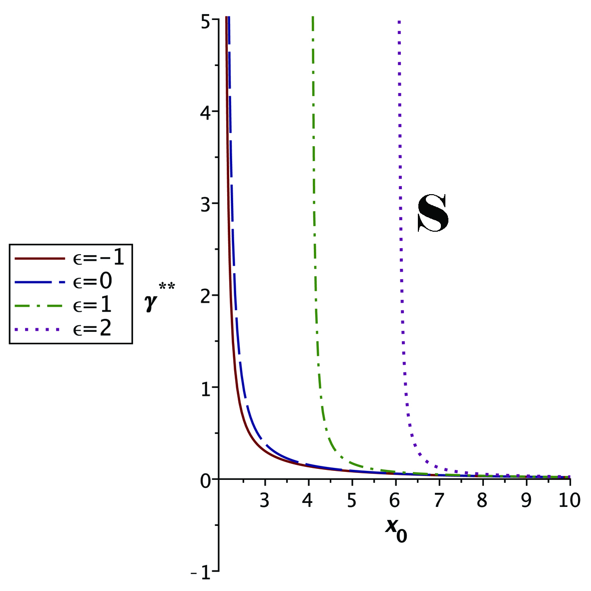
Figure 8: $\gamma^{\ast\ast}$ against $x_{0}$ is plotted for an S-S* ATSW when $\beta^{2}=0$, for four diverse values of $\epsilon$. Again, $\epsilon=-1$ and $\epsilon=0$ are related to an S-M ATSW and an S-S TSW, respectively. A sign S implies the stable region.

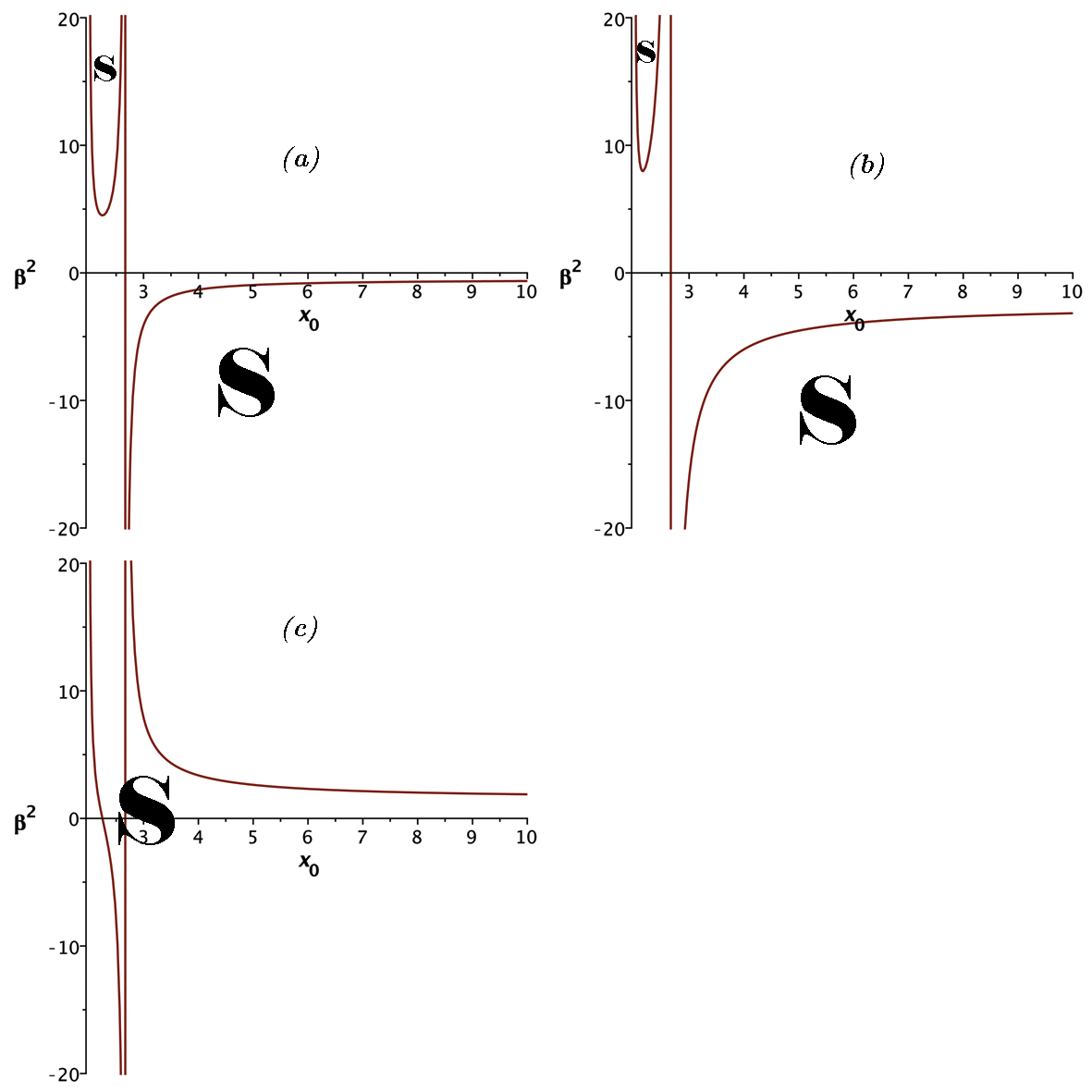
Figure 9: For an S-ERN ATSW, the plot of $\beta^{2}$ against $x_{0}$ are compared for the cases $a)$ $\gamma_{a}=0$, $b)$ $\gamma_{b}=-1/\pi M^{2}x_{0}^{2}$, and $c)$ $\gamma_{c}=1/\pi M^{2}x_{0}^{2}$. Once more, for a positive $\gamma$ the wormhole seems to be more stable than a zero $\gamma$, which itself is more stable than a negative $\gamma$.

V An S-RN TSW

Finally, let us investigate the behavior of an ATSW which connects two inherently different spacetimes; A Schwarzschild geometry with a central mass $M$ and a RN geometry with a central mass $\left(1+\epsilon\right)M$ and a non-zero total charge $Q$. Hereupon, we demand

$$\left\{\begin{array}[]{c}k_{i}=1\\ m_{1}=M\\ m_{2}=(1+\epsilon)M\\ q_{1}=0\\ q_{2}=Q\end{array}\right.$$ (44)

for the two sides’ spacetimes. Since within the framework of natural units hired here the mass and the charge have the same dimension of length, we are allowed to express $Q$ in terms of $M$ in the fashion $Q=\zeta M$, where $\zeta$ is a real number. Inserting all these into Eq. (23) results in an expression for $V_{\text{eff}}$ in terms of $a_{0}$, $\epsilon$, $\zeta$, $\beta^{2}$, $\gamma$ and $M$. Equating $V_{\text{eff}}$ to zero, one can untangle $\beta^{2}$ in terms of the remaining parameters. Needless to say, interplaying with the parameters included can produce a huge number of combinations, each having the potential to be the subject for a separate detailed study in the future. However, here in this brief account, we wrap it up with a single example of a very specific case in which $\epsilon=0$ and $\zeta=1$; accordingly, $m_{1}=m_{2}=q_{2}=M$. Evidently, this grants the special case of Extremal Reissner-Nordström (ERN) geometry for the destined spacetime. Hence, in the general case of a radius-dependent pressure $\left(\gamma\neq 0\right)$, the expression for $\beta^{2}$ reduces to

$$\beta^{2}=-\frac{3\left(x_{0}-2\right)\sqrt{x_{0}\left(x_{0}-2\right)}+x_{0}}{2\left(x_{0}-2\right)\left(3x_{0}-8\right)}+\\ \frac{4\pi M^{2}x_{0}^{3}\gamma\left[\left(-x_{0}+3\right)\sqrt{x_{0}\left(x_{0}-2\right)}+\left(x_{0}-2\right)^{2}\right]}{3x_{0}-8},$$ (45)

where in analogy with the previous section, $x_{0}\equiv\frac{a_{0}}{M}$. Surprisingly, for $\gamma=0$, this $\beta^{2}$ depicts the same general configuration as the one in the previous section. This becomes even more interesting when it is observed that this seemingly similar shape repeats itself for other permitted values of $\epsilon$ and $\zeta$ as well. At this point, the subtle reader would note that $\zeta=0$ recovers the discussions represented in the previous section. Fig. 9 illustrates Eq. (43) for $\beta^{2}$ against $x_{0}$ for three selected functions of $\gamma$. These three functions are chosen as such, so the deduced diagrams can be comparable to the ones of the previous section, namely

$$\gamma_{a}=0,$$

$$\gamma_{b}=\frac{-1}{\pi M^{2}x_{0}^{2}},$$

and

$$\gamma_{c}=\frac{1}{\pi M^{2}x_{0}^{2}}.$$

VI Conclusion

In the context of linear stability analysis of TSWs, the wormhole under study has always been assumed to be symmetric. In this study, however, this presumption is broken by introducing a new kind of wormholes; ATSWs. To show that the stability of such peculiar objects can be studied in the context of linear stability analysis, we have established a general formulation which was used in the next sections to examine three distinct cases: an ATSW between two cosmic string universes of different deficit angles, an ATSW connecting two Schwarzschild geometries of different central masses, and finally we stepped further to study the stability of an ATSW connecting two spacetimes of different natures; Schwarzschild and Reissner-Nordström. This list can easily be expanded in future works. We have shown that these objects, with an exotic perfect fluid of EoS $p=p(\sigma,a)$ on their surfaces, can be stable. The effective potential of the problem acceptedly has a more intricate structure compared with the symmetric wormholes. Two critical parameters, $\beta^{2}=\frac{\partial p}{\partial\sigma}$ and $\gamma=-\frac{\partial p}{\partial a}$, are introduced and analyzed for each given source in connection with the effective potential. By graphing their stability diagrams, we qualitatively examined the stability under various conditions, compared them with each other, and counted some similarities and differences with the special cases of symmetric TSWs. Most importantly, it was observed that in case of a barotropic EoS, the stability diagrams maintain their general shapes, consisting of a bowl-like branch followed by an asymptotically zero-seeking branch. Comparing the diagrams, it was stated that in case of barotropic EoS, the thin-shell wormholes studied here, are most stable at their symmetries. By this, it is meant that for the regions of stability where $\beta^{2}$ is positive and hence physically meaningful, the area tends to shrink with any deviation from the symmetry. Nevertheless, an analytical study can shed more light upon this. Moreover, in the case of a variable EoS, the general form of the function $\gamma$ is proved to be crucial, and can highly manipulate the expected universal gesture of the stability diagram mentioned above. However, since choices for the functions of $\gamma$ were up to an arbitrary factor, a precise numerical and/or analytical assessment is needed to show the full influence of this pressure’s radial-dependency on the stability of ATSWs.

VII Appendix

In section $IV$, the effective potential for an S-S* ATSW was discussed traditionally based on the corresponding graphs of $\beta^{2}$ against $x_{0}$. Nonetheless, the rather unpleasant forms of $V_{\text{eff}}$ and $\beta^{2}$ are given explicitly here, for the sake of completeness.

The potential is expressed as follows

$$V_{\text{eff}}\left(x,\epsilon,\beta^{2},\gamma\right)=\frac{1}{M^{2}x_{0}^{3}\left(x_{0}-2\right)\left[x_{0}-2\left(\epsilon+1\right)\right]\left[\sqrt{x_{0}-2}+\sqrt{x_{0}-2\left(\epsilon+1\right)}\right]^{4}}\times\\ \left\{x_{0}\sqrt{x_{0}-2\left(\epsilon+1\right)}\left\{\left[-16\left(2\beta^{2}+1\right)x_{0}^{4}+8\left(18\beta^{2}+7\right)\left(\epsilon+2\right)x_{0}^{3}-4\left[\left(46\beta^{2}+15\right)\epsilon^{2}+4\left(60\beta^{2}+19\right)\left(\epsilon+1\right)\right]x_{0}^{2}\right.\right.\right.\\ \left.+4\left[3\left(4\beta^{2}+1\right)\epsilon^{2}+16\left(11\beta^{2}+3\right)\left(\epsilon+1\right)\right]\left(\epsilon+2\right)x_{0}-24\left(4\beta^{2}+1\right)\left(\epsilon^{2}+8\epsilon+8\right)\left(\epsilon+1\right)\right]\sqrt{\left(x_{0}-2\right)}\\ \left.+32\pi\gamma M^{2}\left[x_{0}-2\left(1+\epsilon\right)\right]\left(x_{0}-2\right)^{2}\left(2x_{0}-3\epsilon-2\right)x_{0}^{3/2}\right\}\\ +32\pi\gamma M^{2}\left[x_{0}-2\left(1+\epsilon\right)\right]\left(x_{0}-2\right)^{3/2}\left(2x_{0}-3\epsilon-2\right)^{2}x_{0}^{5/2}\\ -16\left(2\beta^{2}+1\right)x^{5}+8\left(22\beta^{2}+9\right)\left(\epsilon+2\right)x_{0}^{4}\\ -12\left[\left(26\beta^{2}+9\right)\epsilon^{2}+4\left(32\beta^{2}+11\right)\left(\epsilon+1\right)\right]x_{0}^{3}\\ +4\left[\left(44\beta^{2}+13\right)\epsilon^{3}+6\left(84\beta^{2}+25\right)\epsilon^{2}+4\left(3\epsilon+2\right)\left(104\beta^{2}+31\right)\right]x_{0}^{2}\\ \left.-32\left(\epsilon+1\right)\left[\left(23\beta^{2}+6\right)\epsilon^{2}+2\left(56\beta^{2}+15\right)\left(\epsilon+1\right)\right]x_{0}+192\left(4\beta^{2}+1\right)\left(\epsilon+1\right)^{2}\left(\epsilon+2\right)\right\};$$ (46)

while for $\beta^{2}$ solving $V_{\text{eff}}=0$ gives rise to

$$\beta^{2}=\frac{1}{2\epsilon\left(x_{0}-2\right)\left[x_{0}-2\left(1+\epsilon\right)\right]\left(4x_{0}^{2}-9x_{0}\epsilon-18x_{0}+18\epsilon+18\right)}\times\\ \left\{x_{0}\sqrt{x_{0}-2\left(1+\epsilon\right)}\left[-2\sqrt{x_{0}-2}\epsilon\left(x_{0}^{2}-\frac{3}{2}\left(\epsilon+2\right)x_{0}+\frac{3}{2}\left(\epsilon+1\right)\right)\right.\right.\\ \left.-8\pi M^{2}\eta x_{0}^{3/2}\left(x_{0}-2\right)^{2}\left[x_{0}-2\left(1+\epsilon\right)\right]\left[x_{0}-3\left(1+\epsilon\right)\right]\right]\\ +8\pi M^{2}\eta x_{0}^{5/2}\left(x_{0}-2\right)^{3/2}\left(x_{0}-3\right)\left[x_{0}-2\left(1+\epsilon\right)\right]^{2}\\ \left.-2\epsilon\left[x_{0}^{4}-4\left(1+\epsilon\right)x_{0}^{3}+\frac{3}{2}\left(3\epsilon^{2}+17\epsilon+17\right)x_{0}^{2}-18\left(\epsilon^{2}+3\epsilon+2\right)x_{0}+18\left(1+\epsilon\right)^{2}\right]\right\}.$$ (47)

References

- (1) L. Flamm, Physikalische Zeitschrift 17, 448 (1916).
- (2) A. Einstein and N. Rosen, Phys. Rev. 48, 73 (1935).
- (3) M. S. Morris and K. S. Thorne, Am. J. Phys. 56, 395 (1988); M. S. Morris, K. S. Thorne and U. Yurtsever, Phys. Rev. Lett. 61, 1446 (1988).
- (4) M. Visser, Phys. Rev. D 39, 3182 (1989); M. Visser, Nucl. Phys. H 328, 203 (1989).
- (5) P. R. Brady, J. Louko and E. Poisson, Phys. Rev. D 44, 1891 (1991); E. Poisson and M. Visser, Phys. Rev. D 52, 7318 (1995); M. Visser, Lorentzian Wormholes from Einstein to Ha-voking (American Institute of Physics, New York, 1995).
- (6) E. F. Eiroa and G. F. Aguirre, Phys. Rev. D 94, 044016 (2016); E. F. Eiroa and G. F. Aguirre, Eur. Phys. J. C 76, 132 (2016); M. R. Mehdizadeh, M. K. Zangeneh and F. S. N. Lobo, Phys. Rev. D 92, 044022 (2015); T. Kokubu and T. Harada, Class. Quant. Grav. 32, 205001 (2015); M. Sharif and M. Azam, Eur. Phys. J. C 73, 2407 (2013); N. M. Garcia, F. S. N. Lobo and M. Visser, Phys. Rev. D 86, 044026 (2012); M. H. Dehghani and M. R. Mehdizadeh, Phys. Rev. D 85, 024024 (2012); X. Yue and S. Gao, Phys. Lett. A 375, 2193 (2011); S. V. Sushkov, Phys. Rev. D 71, 043520 (2005);
- (7) M. G. Richarte and C. Simeone, Phys. Rev. D 76, 087502 (2007); Erratum Phys. Rev. D 77, 089903 (2008); T. Bandyopadhyay and S. Chakraborty, Class. Quantum Grav., 26, 085005 (2009); S. H. Mazharimousavi, M. Halilsoy and Z. Amirabi, Class. Quantum Grav., 28, 025004 (2011); S. H. Mazharimousavi and M. Halilsoy, Eur. Phys. J. C 75, 81 (2015); S. H. Mazharimousavi and M. Halilsoy, Eur. Phys. J. C 75, 271 (2015); S. H. Mazharimousavi and M. Halilsoy, Eur. Phys. J. C 75, 540 (2015); M. K. Zangeneh, F. S. N. Lobo and M. H. Dehghani, Phys. Rev. D 92, 124049 (2015).
- (8) F. S. N. Lobo, P. Crawford, Class. Quant. Grav. 22, 4869 (2005); A. Banerjee, K. Jusufi, S. Bahamonde, Grav. Cosmol. 24, 1 (2018); F. S. N. Lobo, P. Crawford, Class. Quant. Grav. 21, 391 (2004); E. F. Eiroa, G. E. Romero, Gen. Rel. Grav. 36, 651 (2004); E. F. Eiroa, C. Simeone, Phys. Rev. D 76, 024021 (2007); G. A. S. Dias, J. P. S. Lemos, Phys. Rev. D 82, 084023 (2010); E. F. Eiroa, Phys. Rev. D 78, 024018 (2008); J. P. S. Lemos, F. S. N. Lobo, Phys. Rev. D 78, 044030 (2008); F. S. N. Lobo, R. Garattini, JHEP 1312, 065 (2013); E. F. Eiroa, C. Simeone, Phys. Rev. D 83, 104009 (2011); X. Yue, S. Gao, Phys. Lett. A 375, 2193 (2011); S. H. Mazharimousavi, M. Halilsoy, Z. Amirabi, Phys. Rev. D 89, 084003 (2014).
- (9) S. Bahamonde, D. Benisty, E. I. Guendelman, arXiv:1801.08334; E. Guendelman, A. Kaganovich, E. Nissimov, S. Pacheva, AIP Conf. Proc. 1243, 60 (2010); C. Hoffmann, T. Ioannidou, S. Kahlen, B. Kleihaus, J. Kunz, Phys. Rev. D 95, 084010 (2017);
- (10) W. Israel, Nuovo Cimento 44B, 1 (1966); V. de la Cruz and W. Israel, Nuovo Cimento 51A, 774 (1967); J. E. Chase, Nuovo Cimento 67B, 136. (1970); S. K. Blau, E. I. Guendelman and A. H. Guth, Phys. Rev. D 35, 1747 (1987); R. Balbinot and E. Poisson, Phys. Rev. D 41, 395 (1990).
- (11) N. M. Garcia, F. S. N. Lobo and M. Visser, Phys. Rev. D 86, 044026 (2012); F. S. N. Lobo, Class. Quant. Grav. 21, 4811 (2004).
- (12) V. Varela, Phys. Rev. D 92, 044002 (2015).
- (13) E. F. Eiroa and G. E. Romero, Gen. Rel. Grav. 36, 651 (2004).