Finite temperature quantum annealing solving exponentially small gap problem with non-monotonic success probability

Abstract

Closed-system quantum annealing is expected to sometimes fail spectacularly in solving simple problems for which the gap becomes exponentially small in the problem size. Much less is known about whether this gap scaling also impedes open-system quantum annealing. Here we study the performance of a quantum annealing processor in solving such a problem: a ferromagnetic chain with sectors of alternating coupling strength that is classically trivial but exhibits an exponentially decreasing gap in the sector size. The gap is several orders of magnitude smaller than the device temperature. Contrary to the closed-system expectation, the success probability rises for sufficiently large sector sizes. The success probability is strongly correlated with the number of thermally accessible excited states at the critical point. We demonstrate that this behavior is consistent with a quantum open-system description that is unrelated to thermal relaxation, and is instead dominated by the system’s properties at the critical point.

I Introduction

Quantum annealing (QA) Apolloni et al. (1989, 1990); Ray et al. (1989); Somorjai (1991); Amara et al. (1993); Finnila et al. (1994); Kadowaki and Nishimori (1998); Das and Chakrabarti (2008), also known as the quantum adiabatic algorithm Farhi et al. (2000, 2001) or adiabatic quantum optimization Smelyanskiy et al. (2001); Reichardt (2004) is a heuristic quantum algorithm for solving combinatorial optimization problems. Starting from the ground state of the initial Hamiltonian, typically a transverse field, the algorithm relies on continuously deforming the Hamiltonian such that the system reaches the final ground state–typically of a longitudinal Ising model—thus solving the optimization problem. In the closed-system setting, the adiabatic theorem of quantum mechanics Kato (1950) provides a guarantee that QA will find the final ground state if the run-time is sufficiently large relative to the inverse of the quantum ground state energy gap Jansen et al. (2007); Lidar et al. (2009). However, this does not guarantee that QA will generally perform better than classical optimization algorithms. In fact, it is well known that QA, implemented as a transverse field Ising model, can result in dramatic slowdowns relative to classical algorithms even for very simple optimization problems van Dam et al. (2001); Reichardt (2004); Farhi et al. (2008); Jörg et al. (2008); Laumann et al. (2012). Generally, this is attributed to the appearance of exponentially small gaps in such problems Albash and Lidar (2018a).

A case in point is the ferromagnetic Ising spin chain with alternating coupling strength and open boundary conditions studied by Reichardt Reichardt (2004). The ‘alternating sectors chain’ (ASC) of length $N$ spins is divided into equally sized sectors of size $n$ of ‘heavy’ couplings $W_{1}$ and ‘light’ couplings $W_{2}$, with $W_{1}>W_{2}>0$. Since all the couplings are ferromagnetic, the problem is trivial to solve by inspection: the two degenerate ground states are the fully-aligned states, with all spins pointing either up or down. However, this simple problem poses a challenge for closed-system QA since the transverse field Ising model exhibits an exponentially small gap in the sector size $n$ Reichardt (2004), thus forcing the run-time to be exponentially long in order to guarantee a constant success probability. A related result is that QA performs exponentially worse than its imaginary-time counterpart for disordered transverse field Ising chains with open boundary conditions Zanca and Santoro (2016), where QA exhibits an infinite-randomness critical point Fisher (1995).

As a corollary, we may naively expect that for a fixed run-time, the success probability will decrease exponentially and monotonically with the sector size. While such a conclusion does not follow logically from the adiabatic theorem, it is supported by the well-studied Landau-Zener two-level problem Landau (1932); Zener (1932); Joye (1994). How relevant are such dire closed-system expectations for real-world devices? By varying the sector size of the ASC problem on a physical quantum annealer, we find a drastic departure from the above expectations. Instead of a monotonically decreasing success probability (at constant run-time), we observe that the success probability starts to grow above a critical sector size $n^{\ast}$, which depends mildly on the chain parameters $(W_{1},W_{2})$. We explain this behavior in terms of a simple open-system model whose salient feature is the number of thermally accessible states from the instantaneous ground state at the quantum critical point. The scaling of this ‘thermal density of states’ is non-monotonic with the sector size and peaks at $n^{\ast}$, thus strongly correlating with the success probability of the quantum annealer. Our model then explains the success probability behavior as arising predominantly from the number of thermally accessible excitations from the ground state, and we support this model by adiabatic master equation simulations.

Our result does not imply that open-system effects can lend an advantage to QA, and hence it is different from proposed mechanisms for how open system effects can assist QA. For example, thermal relaxation is known to provide one form of assistance to QA Childs et al. (2001); Sarandy and Lidar (2005); Amin et al. (2008); Venuti et al. (2017), but our model does not use thermal relaxation to increase the success probability above $n^{\ast}$. We note that Ref. Amin et al. (2008) introduced the idea that significant mixing due to open system effects (beyond relaxation) at an anti-crossing between the first excited and ground states could provide an advantage, and its theoretical predictions were supported by the experiments in Ref. Dickson et al. (2013). In Ref. Amin et al. (2008) an analysis of adiabatic Grover search was performed (a model which cannot be experimentally implemented in a transverse field Ising model), along with numerical simulations of random field Ising models. In contrast, here we treat an analytically solvable model that is also experimentally implementable using current quantum annealing hardware.

We also compare our empirical results to the predictions of the classical spin-vector Monte Carlo model Shin et al. (2014a), and find that it does not adequately explain them. Our study lends credence to the notion that the performance of real-world QA devices can differ substantially from the scaling of the quantum gap.

II Result

II.1 The alternating sectors chain model

We consider the transverse Ising model with a time-dependent Hamiltonian of the form:

$$H(s)=-A(s)\sum_{i=1}^{N}\sigma_{i}^{x}+B(s)H_{\text{ASC}}\ ,$$ (1)

where $t_{\mathrm{f}}$ is the total annealing time, $s=t/t_{\mathrm{f}}\in[0,1]$, and $A(s)$ and $B(s)$ are the annealing schedules, monotonically decreasing and increasing, respectively, satisfying $B(0)=0$ and $A(1)=0$. The alternating sectors chain Hamiltonian is

$$H_{\text{ASC}}=-\sum_{i=1}^{N-1}J_{i}\sigma_{i}^{z}\sigma_{i+1}^{z}\ ,$$ (2)

where for a given sector size $n$ the couplings are given by

$$J_{i}=\begin{cases}W_{1}&\quad\text{if }\lceil i/n\rceil\text{ is odd}\\ W_{2}&\quad\text{otherwise}\end{cases}$$ (3)

Thus the $b+1$ odd-numbered sectors are ‘heavy’ ($J_{i}=W_{1}$), and the $b$ even-numbered sectors are ‘light’ ($J_{i}=W_{2}$) for a total of $2b+1=\frac{N-1}{n}$ sectors. This is illustrated in Fig. 1.

Figure 1: Illustration of an alternating sector chain (ASC). This example has sector size $n=3$, length $N=10$ and number of sectors $2b+1=3$. Red lines denote the heavy sector with coupling $W_{1}$, blue lines denote the light sector with coupling $W_{2}<W_{1}$.

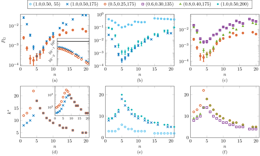
Figure 2: Empirical success probability vs $\bm{k}^{\ast}$ for the ASC problem on the DW2X processor. $k^{\ast}$ denotes the number of single-fermion energies that fall below the thermal energy gap at the point of the minimum gap $s^{\ast}$. The legend entries indicate the chain parameters: ($W_{1}$,$W_{2}$,$N$). The error bars everywhere indicate $95\%$ confidence intervals calculated using a bootstrap over different gauges and embeddings. (a)-(c) Contrary to closed-system theory expectations, the success probability $P_{\text{G}}$ is non-monotonic in the sector size $n$, first decreasing and then increasing, exponentially. Inset (a): The minimum gap (in GHz) of the chains as a function of the sector size $n\in\{1,\dots,20\}$. The solid black line denotes the operating temperature energy scale of the DW2X. (d)-(f) For all chains we studied the ground state success probability has a minimum at the sector size $n^{*}$ where the peak in the number of single-fermion states $k^{\ast}$ occurs [compare with (a)-(c)]. The rise and fall pattern, as well as the location of $n^{*}$, are in agreement with the behavior of $P_{\text{G}}$ within the error bars. Inset (d): The total number of energy eigenstates that fall below the thermal energy gap as a function of the sector size $n$. In this case the peak position does not agree with the ground state success probability minimum.

We briefly summarize the intuitive argument of Ref. Reichardt (2004) for the failure of QA to efficiently solve the ASC problem. Consider the $N\gg 1$ and $n\gg 1$ limit, where any given light or heavy sector resembles a uniform transverse field Ising chain. Each such transverse field Ising chain encounters a quantum phase transition separating the disordered phase and the ordered phase when the strength of the transverse field and the chain coupling are equal, i.e., when $A(s)=B(s)J_{i}$ Sachdev (2011). Therefore the heavy sectors order independently before the light sectors during the anneal. Since the transverse field generates only local spin flips, QA is likely to get stuck in a local minimum with domain walls (antiparallel spins resulting in unsatisfied couplings) in the disordered (light) sectors, if $t_{\mathrm{f}}$ is less than exponential in $n$. We note that this mechanism, in which large local regions order before the whole is well-known in disordered, geometrically local optimization problems, giving rise to a Griffiths phase Fisher (1995).

This argument explains the behavior of a closed-system quantum annealer operating in the adiabatic limit. To check its experimental relevance, we next present the results of tests performed with a physical quantum annealer operating at non-zero temperature.

II.2 Empirical results

As an instantiation of a physical quantum annealer we used a D-Wave 2X (DW2X) processor. We consider ASCs with sector size $n\in[2,20]$. Since the number of sectors $b=(N-1)/n$ must be an integer, the chain length varies slightly with $n$. The minimum gap for these chains is below the processor temperature. Additional details about the processor and of our implementation of these chains are given in Methods.

Figures 2(a)-2(c) show the empirical success probability results for a fixed annealing time $t_{\mathrm{f}}=5\mu$s. Longer annealing times do not change the qualitative behavior of the results, but do lead to changes in the success probability (we provide these results in Appendix G). A longer annealing time can result in more thermal excitations near the minimum gap, but it may also allow more time for ground state repopulation after the minimum gap. The latter can be characterized in terms of a recombination of fermionic excitations by a quantum-diffusion mediated process Smelyanskiy et al. (2017). Unfortunately, we cannot distinguish between these two effects, as we only have access to their combined effect in the final-time success probability.

In stark contrast to the theoretical closed-system expectation, the success probability does not decrease monotonically with sector size, but exhibits a minimum, after which it grows back to close to its initial value. The decline as well as the initial rise are exponential in $n$. Longer chains result in a lower $P_{\text{G}}$ and a more pronounced minimum, but the position of the minimum depends only weakly on the chain parameter values $(W_{1},W_{2})$ (the value of $n^{*}$ shifts to the right as $(W_{1},W_{2})$ are increased) but not on $N$.

What might explain this behavior? Clearly, a purely gap-based approach cannot suffice, since the gap shrinks exponentially in $n$ for the ASC problem Reichardt (2004) [see also the inset of Fig. 2(a)]. However, for all chain parameters we have studied, the temperature is greater than the quantum minimum gap. In this setting not only the gap matters, but also the number of accessible energy levels that fall within the energy scale set by the temperature. In an open-system description of quantum annealing Childs et al. (2001); Amin et al. (2009); Albash et al. (2012); Deng et al. (2013); Ashhab (2014); Albash and Lidar (2015), both the Boltzmann factor $\exp(-\beta\Delta)$ ($\beta$ denotes the inverse temperature and $\Delta$ is the minimum gap) and the density of states determine the excitation and relaxation rates out of and back to the ground state. As we demonstrate next, the features of the DW2X success probability results, specifically the exponential fall and rise with $n$, and the position of the minimum, can be explained in terms of the number of single-fermion states that lie within the temperature energy scale at the critical point.

II.3 Fermionization

We can determine the spectrum of the quantum Hamiltonian [Eq. (1)] by transforming the system into a system of free fermions with fermionic raising and lowering operators $\eta_{k}^{\dagger}$ and $\eta_{k}$ Lieb et al. (1961); Sachdev (2011). The result is Reichardt (2004):

$$H(s)=E_{\mathrm{g}}(s)+\sum_{k=1}^{N}\lambda_{k}(s)\eta_{k}^{\dagger}\eta_{k}\ ,$$ (4)

where $E_{\mathrm{g}}(s)$ is the instantaneous ground state energy and $\{\lambda_{k}(s)\}$ are the single-fermion state energies, i.e., the eigenvalues of the linear system

$$\vec{\Phi}_{k}(s)(\mathbf{A}-\mathbf{B})(\mathbf{A}+\mathbf{B})=\lambda_{k}^{2}(s)\vec{\Phi}_{k}(s)\ ,$$ (5)

where the matrices $\mathbf{A}$ and $\mathbf{B}$ are tridiagonal and are given in Appendix A along with full details of the derivation. The vacuum of the fermionic system $\ket{0}$ is defined by $\eta_{k}\ket{0}=0\ \forall\ k$ and is the ground state of the system. Higher energy states correspond to single and many-particle fermionic excitations of the vacuum. At the end of the anneal, fermionic excitations corresponds to domain walls in the classical Ising chain (see Appendix B).

The Ising problem is $\mathbb{Z}_{2}$-symmetric, so the ground state and the first excited state of the quantum Hamiltonian merge towards the end of evolution to form a doubly degenerate ground state. Since any population in the instantaneous first excited state will merge back with the ground state at the end of the evolution, the relevant minimum gap of the problem is the gap between the ground state and the second excited state: $\Delta(s)=\lambda_{2}(s)$, which occurs at the point $s^{*}=\operatorname*{argmin}_{s\in[0,1]}\Delta(s)$. In the thermodynamic limit, this point coincides with the quantum critical point where the geometric mean of the Ising fields balances the transverse field, $A(s^{\ast})=\sqrt{W_{1}W_{2}}B(s^{\ast})$ Hermisson et al. (1997); Pfeuty (1979). Henceforth we write $\Delta\equiv\Delta(s^{*})$ for the minimum gap.

II.4 Spectral analysis

Let $k^{\ast}$ be the number of single-fermion states with energy smaller than the thermal gap at the critical point, i.e.,

$$k^{\ast}=\operatorname*{argmax}_{k}\Big{\{}\lambda_{k}(s^{\ast})<T\Big{\}}\ .$$ (6)

As can be seen by comparing Figs. 2(d)-2(f) to Figs. 2(a)-2(c), we find that the behavior of $k^{\ast}$ correlates strongly with the ground state success probability for all ASC cases we tested, when we set $T=12\ \text{mK}=1.57$ GHz, the operating temperature of the DW2X processor (we use $k_{\mathrm{B}}=\hbar=1$ units throughout). Specifically, $k^{\ast}$ peaks exactly where the success probability is minimized, which strongly suggests that $k^{\ast}$ is the relevant quantity explaining the empirically observed quantum annealing success probability. Longer chains result in a larger value of $k^{\ast}$ and a more pronounced maximum. Of all the ASC sets we tried, we only found a partial exception to this rule for the case $(1,0.5,200)$, where $k^{\ast}$ peaks at $n^{\ast}=5$ [Fig. 2(e)] but the empirical success probability for $n=5$ and $n=6$ is roughly the same [Fig. 2(b)]. We show later that this exception can be resolved when the details of the energy spectrum are taken into account via numerical simulations.

In contrast, the total number of energy eigenstates (including multi-fermion states) that lie within the thermal gap $[E_{\textrm{g}}(s^{\ast}),E_{\textrm{g}}(s^{\ast})+T]$, while rising and falling exponentially in $n$ like the empirical success probability in Fig. 2(a), does not peak in agreement with the peak position of the latter [see the inset of Fig. 2(d)].

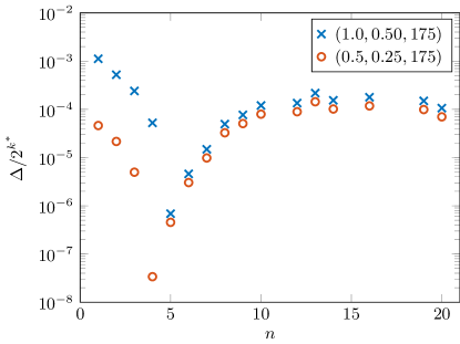
Figure 3: Ratio of the gap to the thermal density of states, as a function of sector size. Two alternating sector chain cases are shown. The position of the minimum is determined by $d$ rather than $\Delta$, as can be seen by comparing to Fig. 2(d) where the plot of $d=2^{k^{\ast}}$ alone correlates well with the position of minima in the empirical success probability curves.

Why and how does the behavior of $k^{*}$ explain the value of $n^{*}$? Heuristically, we expect the success probability to behave as

$$P_{\mathrm{G}}\sim\frac{1-e^{-\beta\Delta}}{d}\ ,$$ (7)

where $d$ is the ‘thermal density of states’ at the critical point $s^{*}$. Note that the role of the gap here is different from the closed-system case, since we are assuming that thermal transitions dominate over diabatic ones, so that the gap is compared to the temperature rather than the annealing time. Contrast this with the closed system case, where the Landau-Zener formula for closed two-level systems and Hamiltonians analytic in the time parameter (subject to a variety of additional technical conditions) states that: $P_{\mathrm{G}}\sim 1-e^{-\eta\Delta^{2}t_{\mathrm{f}}}$, where $\eta$ is a constant with units of time that depends on the parameters that quantify the behavior at the avoided crossing (appearing in, e.g., the proof of Theorem 2.1 in Ref. Joye (1994)). Since then $P_{\mathrm{G}}=O(\eta\Delta^{2}t_{\mathrm{f}})$, we expect the success probability to decrease exponentially at constant run-time $t_{\mathrm{f}}$ if the gap shrinks exponentially in the system size.

Our key assumption is that the thermal transitions between states differing by more than one fermion are negligible. That is, thermal excitation (relaxation) only happens via creation (annihilation) of one fermion at a time (see Appendix C for a detailed argument). Additionally, the Boltzmann factor suppresses excitations that require energy exchange greater than $\lambda_{k^{\ast}}$. Starting from the ground state, all single-fermion states with energy $\leq E_{\mathrm{g}}+\lambda_{k^{\ast}}$ are populated first, followed by all two-fermion states with total energy $\leq E_{\mathrm{g}}+\lambda_{k^{\ast}}+\lambda_{k^{\ast}-1}$, etc. In all, $\sum_{k=1}^{k^{*}}\binom{k^{*}}{k}=2^{k^{\ast}}-1$ excited states are thermally populated in this manner. Thus $d\leavevmode\nobreak\ \sim 2^{k^{\ast}}$ states are thermally accessible from the ground state.

For a sufficiently small gap we have $1-e^{-\beta\Delta}\sim\beta\Delta$, so that $P_{\mathrm{G}}\sim\beta\Delta/d$. As can be seen from Figs. 2(d)-2(f), $k^{*}$ rises and falls steeply for $n<n^{*}$ and $n>n^{*}$ respectively. For the ASCs under consideration, $d$ varies much faster with $n$ than the gap $\Delta$ (see Fig. 3). Thus $P_{\mathrm{G}}\sim 2^{-k^{\ast}}$. This argument explains both the observed minimum of $P_{\mathrm{G}}$ at $n^{*}$ and the exponential drop and rise of $P_{\mathrm{G}}$ with $n$, in terms of the thermal density of states. In Appendix D we give a more detailed argument based on transition rates obtained from the adiabatic master equation, which we discuss next.

II.5 Master equation model

We now consider a simplified model of the open system dynamics in order to make numerical predictions. We take the evolution of the populations $\vec{p}=\{p_{a}\}$ in the instantaneous energy eigenbasis of the system to be described by a Pauli master equation Pauli (1928). The form of the Pauli master equation is identical to that of the adiabatic Markovian quantum master equation Albash et al. (2012), derived for a system of qubits weakly coupled to independent identical bosonic baths. The master equation with an Ohmic bosonic bath has been successfully applied to qualitatively (and sometimes quantitatively) reproduce empirical D-Wave data Albash et al. (2015a); Boixo et al. (2013); Albash et al. (2015b, c). However, it does not account for $1/f$ noise Yoshihara et al. (2006), which may invalidate the weak coupling approximation when the energy gap is smaller than the temperature Boixo et al. (2016).

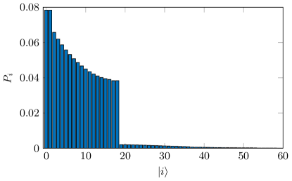
(a)  

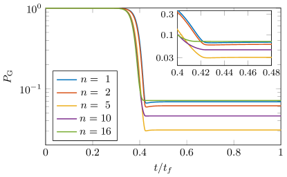
(b)  

Figure 4: Master equation results for the state populations when restricting the excited states to single-fermion states. (a) The population in each single-fermion state at $t=t_{\mathrm{f}}$ in a one-fermion simulation. The chain parameters are $N=176$, $W_{1}=1$, $W_{2}=0.5$, $t_{\mathrm{f}}=5\mu\text{s}$, and $n=5$. With the annealing schedule given in Methods, the quantum minimum gap is at $s^{\ast}=t^{\ast}/t_{\mathrm{f}}\approx 0.424$. At this point we find $k^{\ast}=18$ single-fermion states below the thermal energy $T=12\text{mK}$ (D-Wave processor operating temperature). As expected, in one-fermion simulations, most of the population is found in the first $k^{*}$ states. A long tail of more energetic single particle states beyond the first $k^{*}$ retain some population. (b) Evolution of the instantaneous ground state populations for ASCs with the same parameters as in (a), but for different sector sizes $n$ and with two-fermion states. The ground state loses the majority of its population as it approaches the minimum gap point at $t/t_{\mathrm{f}}=s^{\ast}$. The largest drop is found for $n=n^{*}=5$. Inset: Magnification of the region around the minimum gap. Relaxation plays essentially no role. Instead, the population freezes almost immediately.

After taking diagonal matrix elements and restricting just to the dissipative (non-Hermitian) part one obtains the Pauli master equation Pauli (1928) describing the evolution of the population $\vec{p}=\{p_{a}\}$ in the instantaneous energy eigenbasis of the system Albash and Lidar (2015):

$$\frac{\partial{p}_{a}}{\partial t}=\sum_{b\neq a}\gamma(\omega_{ba})M_{ab}p_{b}-\sum_{b\neq a}\gamma(\omega_{ab})M_{ba}p_{a}\ .$$ (8)

Here all quantities are time-dependent and the matrix elements are

$$M_{ab}(s)=\sum_{\alpha=1}^{N}|\braket{a(s)}{\sigma^{z}_{\alpha}}{b(s)}|^{2}\ ,$$ (9)

where we have assumed an independent thermal bath for each qubit $\alpha$ and where the indices $a$ and $b$ run over the instantaneous energy eigenstates of the system Hamiltonian (Eq. 4) in the fermionic representation [i.e., $H(s)\ket{a(s)}=E_{a}(s)\ket{a(s)}$] and $\omega_{ab}=E_{a}-E_{b}$ is the corresponding instantaneous Bohr frequency. Since the basis we have written this equation in is time-dependent, there are additional terms associated with the changing basis Albash et al. (2012), but we ignore these terms here since we are assuming that the system is dominated by the dissipative dynamics associated with its interaction with its thermal environment.

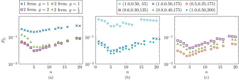
Figure 5: Master equation results for the ground state population when restricting the excited states to single and two fermion states. (a) The result of simulating the ASC problem with parameters $(1,0.5,175)$ via the adiabatic Pauli master equation (8), restricted to the vacuum + single-fermion states, and vacuum + single-fermion + two-fermion states. Also shown is the dependence on the system-bath coupling parameter $g$ in the two-fermion case; doubling it has little impact, whereas halving it increases the success probability somewhat for $n<14$. The position of the minimum at $n^{*}=5$ matches the empirical result seen in Fig. 2(a), except when $g=1/2$, i.e., the position is robust to doubling $g$ but not to halving it. Panels (b) and (c) show additional $2$-fermion master equation results with $g=1$. Note that for the $(1,0.5,200)$ chain, these simulations exhibit better agreement with the DW2X data than the simple $k^{*}$ analysis plotted in Figs. 2(d)-2(f). This is because the simulations also keep track of the Boltzmann factor.

The rates $\gamma(\omega)$ satisfy the quantum detailed balance condition Haag et al. (1967); Breuer and Petruccione (2002), $\gamma(-\omega)=e^{-\beta\omega}\gamma(\omega)$, where $\omega\geq 0$. In our model each qubit is coupled to an independent pure-dephasing bath with an Ohmic power spectrum:

$$\gamma(\omega)=\ 2\pi\eta g^{2}\frac{\omega e^{-|\omega|/\omega_{c}}}{1-e^{-\beta\omega}}\ ,$$ (10)

with UV cutoff $\omega_{c}=8\pi$ GHz and the dimensionless coupling constant $\eta g^{2}=1.2\times 10^{-4}$. The choice for the UV cutoff satisfies the assumptions made in the derivation of the master equation in the Lindblad form Albash et al. (2012). Note that we do not adjust any of the master equation parameter values, which are taken from Ref. Albash et al. (2015a). Details about the numerical solution procedure are given in Methods, and in Appendix E we also confirm that the validity conditions for the derivation of the master equation are satisfied for a relevant range of $n$ values given the parameters of our empirical tests.

Numerically solving the master equation while accounting for all thermally populated $2^{k^{\ast}}$ states is computationally prohibitive, but we can partly verify our interpretation by restricting the evolution of the system described in Eq. (8) to the vacuum and single-fermion states. This is justified in Appendix C, where we show that transitions between states differing by more than a single fermion are negligible. In other words, the dominant thermal transitions occur from the vacuum to the single-fermion states, from the single-fermion states to the two-fermion states, etc. The restriction to the vacuum and single-fermion states further simplifies the master equation (8) to:

$$\dot{p}_{0} =\sum_{b}\gamma(\lambda_{b})M_{b}p_{b}-p_{0}\sum_{b}\gamma(-\lambda_{b})M_{b}$$ (11)

$$\dot{p}_{i} =\gamma(-\lambda_{i})M_{i}p_{0}-\gamma(\lambda_{i})M_{i}p_{i}\ ,$$ (12)

where $\left\{p_{b}\right\}_{b=1}^{N}$ are the single-particle fermion energy populations and $\left\{\lambda_{b}\right\}$ their energies found by solving Eq. (5), and $M_{ab}$ [Eq. (9)] becomes $M_{b}=\sum_{\alpha=1}^{N}|\braket{0}{\sigma^{z}_{\alpha}}{b}|^{2}$. For a better approximation that accounts for more states, we can also perform a two-fermion calculation where we keep the vacuum, the first $k^{\ast}$ one fermion-states and the next $k^{\ast}(k^{\ast}-1)/2$ two fermion states. For two-fermion simulations the master equation becomes Eqs. 11 and 12 along with

$$\dot{p}_{i}={} \gamma(-\lambda_{i})M_{i}p_{0}-\gamma(\lambda_{i})M_{i}p_{i}$$

$$+\sum_{j\neq i}\gamma(\lambda_{j})M_{j}p_{ij}-p_{i}\sum_{j\neq i}\gamma(-\lambda_{i})M_{j}$$ (13)

$$\dot{p}_{ij}={} \gamma(-\lambda_{i})M_{i}p_{j}+\gamma(-\lambda_{j})M_{j}p_{i}-\gamma(\lambda_{i})M_{i}p_{ij}$$

$$-\gamma(\lambda_{j})M_{j}p_{ij}\ ,$$ (14)

where all summations run from $1$ to $k^{\ast}$, and $p_{ij}$ denotes the population in the two-particle fermion energy state $\eta_{i}^{\dagger}\eta_{j}^{\dagger}\ket{0}$.

We can now numerically solve this system of equations. As seen in Fig. 4(a), where we plot the final populations in the different single particle fermion states at $t=t_{\mathrm{f}}$ for one-fermion simulations, only the first $k^{*}$ single-fermion levels are appreciably populated. This agrees with our aforementioned assumption that states with energy greater than $\lambda_{k^{*}}$ are not thermally populated. In Fig. 4(b) we plot the population in the instantaneous ground state as a function of time for two-fermion simulations. The system starts in the gapped phase where the ground state population is at its chosen initial value of $1$. The ground state rapidly loses population via thermal excitation as the system approaches the critical point, after which the population essentially freezes, with repopulation via relaxation from the excited states essentially absent (see inset). Thus, it is not relaxation that explains the increase in ground state population seen in Fig. 2(a)-(c) for $n>n^{*}$. Instead, we find that the ground state population drops most deeply for $n=n^{*}$. This, in turn, is explained by the behavior of $k^{*}$ seen in Fig. 2(d)-(f), as discussed earlier.

We show in Fig. 5 the predicted final ground state population under the one and two-fermion restriction. This minimal model already reproduces the correct location of the minimum in $P_{\text{G}}$. It also reproduces the non-monotonic behavior of the success probability. It does not correctly reproduce the exponential fall and rise. However, including the two-fermion states gives the right trend: it leads to a faster decrease and increase in the population without changing the position of the minimum, suggesting that a simulation with the full $2^{k^{\ast}}$ states would recover the empirically observed exponential dependence of the ground state population seen in Fig. 2(a)-2(c).

III Discussion

A commonly cited failure mode of closed-system quantum annealing is the exponential closing of the quantum gap with increasing problem size. It is expected, on the basis of the Landau-Zener formula and the quantum adiabatic theorem, that to keep the success probability of the algorithm constant the run-time should increase exponentially. As a consequence, one expects the success probability to degrade at constant run-time if the gap decreases with increasing problem size. Our goal in this work was to test this failure mode in an open-system setting where the temperature energy scale is always larger than the minimum gap. We did so by studying the example of a ferromagnetic Ising chain with alternating coupling-strength sectors, whose gap is exponentially small in the sector size, on a quantum annealing device. Our tests showed that while the success probability initially drops exponentially with the sector size, it recovers for larger sector sizes. We found that this deviation from the expected closed-system behavior is qualitatively and semi-quantitatively explained by the system’s spectrum around the quantum critical point. Specifically, the scaling of the quantum gap alone does not account for the behavior of the system, and the scaling of the number of energy eigenstates accessible via thermal excitations at the critical point (the thermal density of states) explains the empirically observed ground state population.

Does there exist a classical explanation for our empirical results? We checked and found that the spin vector Monte Carlo (SVMC) model Shin et al. (2014a) is capable of matching the empirical DW2X results provided we fine-tune its parameters for each specific chain parameter set $\{W_{1},W_{2},N\}$. However, it does not provide as satisfactory a physical explanation of the empirical results as the fermionic or master equation models, which require no such fine-tuning; see Appendix F for details.

Our work demonstrates that care must be exercised when inferring the behavior of open-system quantum annealing from a closed-system analysis of the scaling of the gap. It has already been pointed out that quantum relaxation can play a beneficial role Childs et al. (2001); Sarandy and Lidar (2005); Amin et al. (2008); Dickson et al. (2013); Venuti et al. (2017). However, we have shown that relaxation plays no role in the recovery of the ground state population in our case. Instead, our work highlights the importance of a different mechanism: the scaling of the number of thermally accessible excited states. Thus, to fully assess the prospects of open-system quantum annealing, this mechanism must be understood along with the scaling of the gap and the rate of thermal relaxation. Of course, ultimately we only expect open-system quantum annealing to be scalable via the introduction of error correction methods Young et al. (2013); Jordan et al. (2006); Marvian and Lidar (2017); Jiang and Rieffel (2017).

IV Methods

$N$	174	175	172	173	176	175	176	169
$n$	1	2	3	4	5	6	7	8
$N$	172	171	181	170	183	177	172	181
$n$	9	10	12	13	14	16	19	20

Table 1: Chain length ($N$) and sector size ($n$) for $N\sim 175$.

Alternating sector chains We generated a set of ASCs with chains lengths centered at $N\sim\{55,135,175,200\}$ and with sector sizes $n$ ranging from $2$ to $20$. Since the chain length and sector size must obey the relation $(N-1)/n=2b+1$ with integer $b$, there is some variability in $N$. Table 1 gives the $(N,n)$ pair combinations we used for chain set with mean length $175$.

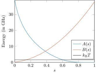
Figure 6: Annealing schedules and temperature. $A(s)$ and $B(s)$ are the annealing schedules of the D-Wave processor used in this work. The fridge temperature (horizontal black line) is $T=12$ mK.

Quantum annealing processor used in this work The D-Wave 2X processor (DW2X) is an $1152$-qubit quantum annealing device made by D-Wave Systems, Inc., using superconducting flux qubits Bunyk et al. (2014). The particular processor used in this study is located at the University of Southern California’s Information Sciences Institute, with $1098$ functional qubits and an operating temperature of $12$ mK. The total annealing time $t_{\mathrm{f}}$ can be set in the range $[5,2000]\ \mu$s. The time-dependent Hamiltonian the processor is designed to implement is given by

$$H(s)=A(s)\sum_{i}\sigma^{z}_{i}+B(s)\left(\sum_{i}h_{i}\sigma_{i}^{z}+\sum_{(i,j)}J_{ij}\sigma_{i}^{z}\sigma_{j}^{z}\right)\ ,$$ (15)

with dimensionless time $s=t/t_{\mathrm{f}}$. Figure 6 describes the annealing schedules $A(s)$ and $B(s)$. The coupling strengths $J_{ij}$ between qubits $i$ and $j$ can be set in the range $[-1,1]$ and the local fields $h_{i}$ can be set in the range $[-2,2]$.

We used $t_{\mathrm{f}}=5\ \mu$s. For each ASC instance we implemented $10$ different embeddings, with $10$ gauge transforms each Boixo et al. (2014). In total, $10^{5}$ runs and readouts were taken per instance. The reported success probability is defined as the fraction of readouts corresponding to a correct ground state. For additional details on the DW2X processor we used see, e.g., Ref. Albash and Lidar (2018b).

Numerical procedure for solving the master equation We solve the coupled differential Eqs. 11, 12, 13 and 14 using a fourth order Runge-Kutta method given by Dormand-Prince Dormand and Prince (1980) with non-negativity constraints Shampine et al. (2005). We compute the transition matrix elements via Eq. 50 and the bath correlation term via Eq. (10).

Data Availability The data that support the findings of this study are available from the corresponding author upon reasonable request.

Appendix A Jordan-Wigner transform

The Jordan-Wigner transform can be used to map a one-dimensional transverse field Ising Hamiltonian to a Hamiltonian of uncoupled (free) fermions. A system of dimension $2^{N}\times 2^{N}$ is thus effectively reduced to a system of dimension $N$, which is essential for our simulations involving $N$ as large as $200$. We briefly summarize the approach found in the classic work of Lieb et al. Lieb et al. (1961).

We start by defining fermionic raising operators $a_{i}^{\dagger}=\frac{1}{2}\left(\otimes_{j=1}^{i-1}\sigma^{x}_{j}\right)(\sigma^{z}_{i}+{i\mkern 1.0mu}\sigma^{y}_{i})$ ($i=1,\dots,N$) and their corresponding lowering operators $a_{i}$. It is easy to check that the fermionic canonical commutation relations are then satisfied: $\{a_{i},a_{j}\}=\{a_{i}^{\dagger},a_{j}^{\dagger}\}=0$ and $\{a^{\dagger}_{i},a_{j}\}=\delta_{ij}$. Rewriting Eq. 1 as

$$H=-\Gamma\sum_{i=1}^{N}\sigma^{x}_{i}-\sum_{i=1}^{N-1}J_{i}\sigma^{z}_{i}\sigma^{z}_{i+1}$$ (16)

and substituting $\sigma^{x}_{i}=1-2a^{\dagger}_{i}a_{i}$, $\sigma^{z}_{i}\sigma^{z}_{i+1}=(a_{i}^{\dagger}-a_{i})(a_{i+1}^{\dagger}+a_{i+1})$ gives

$$H=-N\Gamma+\sum_{ij}a_{i}^{\dagger}A_{ij}a_{j}+\frac{1}{2}(a_{i}^{\dagger}B_{ij}a_{j}^{\dagger}+a_{i}B_{ji}a_{j})\ ,$$ (17)

or

$$H=-N\Gamma+(\vec{a^{\dagger}})^{T}\mathbf{A}\vec{a}+\frac{1}{2}\left[(\mathbf{a^{\dagger}})^{T}\mathbf{B}\mathbf{a^{\dagger}}+\vec{a}^{T}\mathbf{B}^{T}\vec{a}\right]$$ (18)

where $(\vec{a^{\dagger}})^{T}=(a_{1}^{\dagger},\dots,a_{N}^{\dagger})$, $\vec{a}^{T}=(a_{1},\dots,a_{N})$, and

$$\mathbf{A} =\begin{pmatrix}2\Gamma&-J_{1}&0&&\\ -J_{1}&2\Gamma&-J_{2}&&\\ 0&-J_{2}&\ddots&\ddots&0\\ &&\ddots&2\Gamma&-J_{N-1}\\ &\cdots&&-J_{N-1}&2\Gamma\end{pmatrix}\ ,$$ (19)

$$\mathbf{B} =\begin{pmatrix}0&-J_{1}&&&\\ J_{1}&0&-J_{2}&&\\ &J_{2}&\ddots&\ddots&0\\ &&\ddots&0&-J_{N-1}\\ &\cdots&&J_{N-1}&0\end{pmatrix}\ .$$ (20)

The Hamiltonian in Eq. 17 is not fermion number conserving (it contains terms such as $a_{i}^{\dagger}a_{j}^{\dagger}$, which means that $\sum_{i}\sigma^{x}_{i}$ is not conserved), but it can be diagonalized by a Bogoliubov transformation (Lieb et al., 1961, Appendix A) in terms of a new set of fermionic operators $\{\eta_{i},\eta_{i}^{\dagger}\}$:

$$H=E_{\mathrm{g}}+\sum_{i=1}^{N}{\lambda_{i}}\eta_{i}^{\dagger}\eta_{i}\ .$$ (21)

where the $\lambda_{i}$ are the single-fermion energies of the system. The new fermionic operators are real linear combinations of the old ones:

$$\begin{split}\eta_{i}^{\dagger}&=\sum_{k}g_{ik}a^{\dagger}_{k}+\sum_{k}h_{ik}a_{k}\\ \eta_{i}&=\sum_{k}g_{ik}a_{k}+\sum_{k}h_{ik}a^{\dagger}_{k}\ .\end{split}$$ (22)

From Eq. 21 we get

$$\left[\eta_{k},H\right]=\lambda_{k}\eta_{k}\ .$$ (23)

Substituting Eqs. 17 and 22 in Eq. 23 and setting the coefficients of every operator $\{a_{i},a^{\dagger}_{i}\}$ to zero gives

$$\begin{split}\lambda_{k}g_{ki}&=\sum_{j}g_{kj}A_{ji}-h_{kj}B_{ji}\\ \lambda_{k}h_{ki}&=\sum_{j}g_{kj}B_{ji}-h_{kj}A_{ji}\end{split}$$ (24)

Let $\phi_{ik}=g_{ik}+h_{ik}$ and $\psi_{ik}=g_{ik}-h_{ik}$. Plugging this into  Eq. 24, we get two coupled equations:

$$\vec{\Phi}_{k}(\mathbf{A}-\mathbf{B}) =\lambda_{k}\vec{\Psi}_{k}$$ (25)

$$\vec{\Psi}_{k}(\mathbf{A}+\mathbf{B}) =\lambda_{k}\vec{\Phi}_{k}\ ,$$ (26)

where $\vec{\Phi}_{k}=(\phi_{1k},\dots,\phi_{Nk})$ and $\vec{\Psi}_{k}=(\psi_{1k},\dots,\psi_{Nk})$. Eliminating $\vec{\Psi}_{k}$ gives us the decoupled equation,

$$\vec{\Phi}_{k}(\mathbf{A}-\mathbf{B})(\mathbf{A}+\mathbf{B})=\lambda_{k}^{2}\vec{\Phi}_{k}\ .$$ (27)

Solving the eigensystem given by Eq. 27 gives the eigenvalues $\{\lambda_{i}\}$ in the Hamiltonian (21).

We can find the ground state energy $E_{\mathrm{g}}$ by taking trace of Eqs. 17 and 21 (Lieb et al., 1961, Appendix A). From Eq. 17, we have

$$\operatorname{Tr}(H)=2^{N-1}\sum_{i}A_{ii}-2^{N}N\Gamma$$ (28)

and from Eq. 21 we have,

$$\operatorname{Tr}(H)=2^{N-1}\sum_{k}\lambda_{k}+2^{N}E_{\mathrm{g}}\ .$$ (29)

As the trace is invariant under a canonical transform, we get

$$E_{\mathrm{g}}=-N\Gamma+\frac{1}{2}(\sum_{i}A_{ii}-\sum_{k}{\lambda_{k}})=-\frac{1}{2}\sum_{k}\lambda_{k}\ .$$ (30)

If we require that the $\vec{\Phi}_{k}$ are orthonormal, then the transformation given by  Eq. 22 is a canonical transformation. Solving Eq. 25 gives the corresponding $\vec{\Psi}_{k}$.

Finding matrices $\Phi$ and $\Psi$ (and hence $g_{ik}$ and $h_{ik}$) gives the forward transform connecting the undiagonalized fermions to the diagonalized fermions. The inverse transform can be defined as

$$\begin{split}a_{i}^{\dagger}&=\sum_{k}\bar{g}_{ik}\eta^{\dagger}_{k}+\sum_{k}\bar{h}_{ik}\eta_{k}\\ a_{i}&=\sum_{k}\bar{g}_{ik}\eta_{k}+\sum_{k}\bar{h}_{ik}\eta^{\dagger}_{k}\ ,\end{split}$$ (31)

such that

$$\begin{split}a_{i}^{\dagger}+a_{i}&=\sum_{k}\bar{\phi}_{ik}\left(\eta^{\dagger}_{k}+\eta_{k}\right)\\ a_{i}^{\dagger}-a_{i}&=\sum_{k}\bar{\psi}_{ik}\left(\eta^{\dagger}_{k}-\eta_{k}\right)\ ,\end{split}$$ (32)

where $\bar{\phi}_{ik}=\bar{g}_{ik}+\bar{h}_{ik}$ and $\bar{\psi}_{ik}=\bar{g}_{ik}-\bar{h}_{ik}$. Since these transforms are canonical, $\bar{\Phi}=\Phi^{\mathrm{T}}$ and $\bar{\Psi}=\Psi^{\mathrm{T}}$.

Appendix B Fermionic domain-wall states

The eigenstates of the Hamiltonian can be rewritten as many-fermion states. For example, $\ket{0}$ denotes the vacuum which is the ground state of the Hamiltonian, $\ket{a\ b\ c}=\eta^{\dagger}_{a}\eta^{\dagger}_{b}\eta^{\dagger}_{c}\ket{0}$ is a three-fermion state with energy $E_{\mathrm{g}}+\lambda_{a}+\lambda_{b}+\lambda_{c}$ and $\ket{\gamma}=\eta^{\dagger}_{\{\gamma\}}\ket{0}$ is another state with $|\gamma|$ fermions. In this notation $\ket{a\ b\ c}$ means a state with a single fermion in each of the positions $a,b$, and $c$. What do these states look like in the computational basis? We can gain some intuition by considering the special case with zero transverse field.

For $\Gamma=0$, Eq. 27 becomes:

$$\vec{\Phi}_{k}\begin{pmatrix}0&&&&\\ &4J_{1}^{2}&&&\\ &&4J_{2}^{2}&&\\ &&&\ddots&\\ &&&&4J_{N-1}^{2}\end{pmatrix}=\lambda_{k}^{2}\vec{\Phi}_{k}\ .$$ (33)

For simplicity, assume $J_{1}\leq J_{2}\leq\ldots\leq J_{N-1}$. This immediately yields the eigenvalues $\lambda_{1}=0$, $\lambda_{2}=2J_{1}$, $\lambda_{3}=2J_{2}$, $\ldots$, $\lambda_{N}=2J_{N-1}$ and eigenvector

$$\Phi =\begin{pmatrix}1&&&&\\ &1&&&\\ &&1&&\\ &&&\ddots&\\ &&&&1\end{pmatrix}\ .$$ (34)

Using Eq. 26 we find:

$$\Psi =\begin{pmatrix}0&0&0&\ldots&1\\ -1&0&0&\ldots&0\\ 0&-1&0&\ldots&0\\ 0&&\ddots&&0\\ 0&0&\ldots&-1&0\end{pmatrix}\ .$$ (35)

If the $J_{i}$ are not ordered the result remains the same up to a permutation of rows of $\Phi$ and $\Psi$, where the $\lambda_{i}$ are still arranged in ascending order.

Now consider the operator $\sigma^{z}_{i}\sigma^{z}_{i+1}=(a^{\dagger}_{i}-a_{i})(a^{\dagger}_{i+1}+a_{i+1})$ in terms of the diagonalized fermionic operators. Using Eqs. 32, 34 and 35 gives

$$\sigma^{z}_{i}\sigma^{z}_{i+1} =\sum_{kk^{\prime}}\bar{\psi}_{ki}\bar{\phi}_{i+1,k^{\prime}}(\eta^{\dagger}_{k}-\eta_{k})(\eta^{\dagger}_{k^{\prime}}+\eta_{k^{\prime}})$$

$$=\sum_{kk^{\prime}}(-\delta_{k,i+1})(\delta_{k^{\prime},i+1})(\eta^{\dagger}_{k}-\eta_{k})(\eta^{\dagger}_{k^{\prime}}+\eta_{k^{\prime}})$$

$$=1-2\eta^{\dagger}_{i+1}\eta_{i+1}\ .$$ (36)

Thus, the many-fermion states are also the eigenstates of the operators $\sigma^{z}_{i}\sigma^{z}_{i+1}$ with eigenvalue $-1$ if there is a fermion occupying level $i+1$, and eigenvalue $1$ otherwise. In the spin picture, eigenvalue $+1$ denotes a satisfied coupling and $-1$ denotes an unsatisfied coupling. Thus, the presence of a fermion in level $i+1$ can be thought as a domain wall in coupling $i$ of the ferromagnetic chain. The fermionic states $\ket{0}$ and $\ket{1}$ satisfy all the couplings and hence are linear combinations of the all-$0$ and all-$1$ states. This is reflective of the $\mathbb{Z}_{2}$ symmetry inherent in the Ising Hamiltonian, which also manifest itself as $\lambda_{1}=0$. Thus, for given state $\ket{a}$ with energy $E_{a}=E_{\mathrm{g}}+\lambda_{a}$, the state $\ket{a\ 1}$ has the same energy $E_{\mathrm{g}}+\lambda_{a}+\lambda_{1}=E_{a}$. Additionally, $(1-2\eta^{\dagger}_{i+1}\eta_{i+1})\ket{a}=(1-2\eta^{\dagger}_{i+1}\eta_{i+1})\ket{a\ 1}\ \forall\ i\geq 1$ since the fermion occupying the state $\ket{1}$ is not affected by this operation. Ergo, the states $\ket{2}$ and $\ket{2\ 1}$ corresponds to a domain wall at the location of the weakest coupling, $\ket{3}$ and $\ket{3\ 1}$ corresponds to a state with a domain wall at the second weakest coupling, etc. Once the couplers are arranged in alternating sectors such that $J_{1}=J_{2}=\ldots=W_{1}>J_{n+1}=J_{n+2}=\ldots=W_{2}<\ldots$, the domain walls first occur in the light sectors, followed by the heavy sectors, etc.

Appendix C Why states that differ by a single fermionic excitation have the largest matrix elements

In order to determine whether thermal transitions between states can occur, we need to calculate the matrix element of $\sigma^{z}$ between the two states, where we assume that the dominant interaction term between the system and environment is given by a pure dephasing interaction of the form $H_{\mathrm{SB}}=\sum_{i}\sigma^{z}_{i}\otimes B_{i}$ Lanting et al. (2010); Boixo et al. (2016); Albash et al. (2015a, b, a). We we would like to estimate the transition matrix element $\braket{\gamma_{1}}{\sigma^{z}_{i}}{\gamma_{2}}$ between states $\ket{\gamma_{1}}$ and $\ket{\gamma_{2}}$. We shall show that these transitions are most prominent when the states differ by only a single fermion.

In terms of the fermionic operators, the operator $\sigma^{z}$ can be written as

$$\sigma^{z}_{i}=\left[\prod_{j=1}^{i-1}(a_{j}^{\dagger}+a_{j})(a_{j}^{\dagger}-a_{j})\right](a^{\dagger}_{i}+a_{i})$$ (37)

and it can in turn be written in term of the $\{\eta_{k}\}$ and $\{\eta_{k}^{\dagger}\}$ operators using  Eq. 32.

Now consider the matrix element between the vacuum state $\ket{0}$ and the state $\ket{\gamma}$. For the operator $\sigma^{z}_{1}$ we find that

$$\begin{split}\braket{\gamma}{\sigma^{z}_{1}}{0}&=\braket{\gamma}{a^{\dagger}_{1}+a_{1}}{0}\\ &=\braket{\gamma}{\sum_{k}\bar{\phi}_{1k}(\eta^{\dagger}_{k}+\eta_{k})}{0}\\ &=\sum_{k}\bar{\phi}_{1k}\braket{\gamma}{k}.\end{split}$$ (38)

This can only be non-zero if $\ket{\gamma}$ is a single fermion state. Thus, the operator $\sigma^{z}_{1}$ connects the vacuum to single-fermion states.

For $\sigma^{z}_{2}$, we have

$$\begin{split}&\braket{\gamma}{\sigma^{z}_{2}}{0}=\braket{\gamma}{(a^{\dagger}_{1}+a_{1})(a^{\dagger}_{1}-a_{1})(a^{\dagger}_{2}+a_{2})}{0}\\ &=\sum_{k,l,m}\bar{\phi}_{1k}\bar{\psi}_{1l}\bar{\phi}_{2m}\braket{\gamma}{(\eta^{\dagger}_{k}+\eta_{k})(\eta^{\dagger}_{l}+\eta_{l})(\eta^{\dagger}_{m}+\eta_{m})}{0}.\end{split}$$ (39)

For the above term to be non-zero, the state $\ket{\gamma}$ must be either a three-fermion or a single-fermion state. The one-fermion case can be computed in a similar manner to the previous case involving $\sigma_{1}^{z}$, so we focus on the case when $\ket{\gamma}=\ket{a\ b\ c}$ is a three-fermion state. We have

$$\begin{split}&\braket{a\ b\ c}{\sigma^{z}_{2}}{0}\\ &=\sum_{klm}\bar{\phi}_{1k}\bar{\psi}_{1l}\bar{\phi}_{2m}\braket{a\ b\ c}{\eta_{k}^{\dagger}\eta_{l}^{\dagger}\eta_{m}^{\dagger}}{0}\\ &=\sum_{klm}\bar{\phi}_{1k}\bar{\psi}_{1l}\bar{\phi}_{2m}\braket{a\ b\ c}{k\ l\ m}\\ &=\det{\begin{vmatrix}\bar{\phi}_{1a}&\bar{\psi}_{1a}&\bar{\phi}_{2a}\\ \bar{\phi}_{1b}&\bar{\psi}_{1b}&\bar{\phi}_{2b}\\ \bar{\phi}_{1c}&\bar{\psi}_{1c}&\bar{\phi}_{2c}\end{vmatrix}}\ .\end{split}$$ (40)

We find numerically for our problems that the matrix element associated with the three-fermion states is much smaller than that for single-fermion states. For example, for a chain of length $N=176$ with parameters $n=5$, $W_{1}=1$ and $W_{2}=0.5$, we find at $s=s^{\ast}$ that $\braket{3}{\sigma^{z}_{1}}{0}=0.12$ and $\braket{2\ 3\ 4}{\sigma^{z}_{2}}{0}=1.2\times{10}^{-8}$.

Similarly, the matrix element involving $\sigma^{z}_{3}$ requires $\ket{\gamma}$ to be a state with $1$, $3$ or $5$ fermions, etc. We find that the excitation to the $5$-fermion states will be even smaller than that to the $3$-fermion states, since they contain terms that are the product of five terms of the type $\bar{\phi}\bar{\psi}\bar{\phi}\bar{\psi}\bar{\phi}$. Thus, our numerical results indicate that the vacuum state couples predominantly to single-fermion states.

The above analysis can be generalized. Let us consider the matrix element $\theta_{ij}=\braket{0}{\sigma^{z}_{i}}{j}$. Let $\mathbf{\Theta}=[\theta_{ij}]$ and $\mathbf{\bar{\Psi}}=[\bar{\psi}_{ij}]$, and consider $\mathbf{\tilde{G}}=\mathbf{\Theta}\mathbf{\bar{\Psi}}^{\mathrm{T}}$. We have:

$$\tilde{G}_{ij} =\sum_{m}\theta_{im}{\left(\mathbf{\bar{\Psi}}^{\mathrm{T}}\right)}_{mj}$$ (41)

$$=\sum_{m}\bar{\psi}_{jm}\braket{0}{\sigma^{z}_{i}}{m}$$ (42)

$$=\braket{0}{\sigma^{z}_{i}\left(\sum_{m}\bar{\psi}_{jm}(\eta_{m}^{\dagger}-\eta_{m})\right)}{0}$$ (43)

$$=\braket{0}{\sigma^{z}_{i}(a_{j}^{\dagger}-a_{j})}{0}$$ (44)

$$=\braket{0}{A_{1}B_{1}\ldots A_{i-1}B_{i-1}A_{i}B_{j}}{0}\ ,$$ (45)

where we have defined $A_{i}=(a_{i}^{\dagger}+a_{i})$ and $B_{i}=(a_{i}^{\dagger}-a_{i})$. Since the operators $A_{i}$ and $B_{j}$ in Eq. 45 anticommute when they have different indices, we can simplify the expression using Wick’s theorem Wick (1950); Lieb et al. (1961). For a set of anticommutating operators $\{O_{1},O_{2},\ldots,O_{2n}\}$, Wick’s theorem states that

$$\braket{0}{O_{1}O_{2}\ldots O_{2n}}{0}\\ =\sum_{\text{possible pairings}}(-1)^{p}\prod_{\text{all pairs}}\braket{0}{O_{i_{1}}O_{i_{2}}}{0}\ .$$ (46)

where the sum is over all possible pairings of the operators $\{O_{1},O_{2},\ldots,O_{2n}\}$, the product is over the two-point expectation value of all pairs, and $(-1)^{p}$ is the sign of the permutation that is required to bring the paired terms next to each other. For an odd number of operators, the expectation value vanishes. Applying the theorem to Eq. 45, we can make the following simplifications:

$$\braket{0}{A_{i}A_{j}}{0}=\phantom{-}\sum_{k}\bar{\phi}_{ik}\bar{\phi}_{jk}=\delta_{ij}\ ,$$ (47)

$$\braket{0}{B_{i}B_{j}}{0}=-\sum_{k}\bar{\psi}_{ik}\bar{\psi}_{jk}=-\delta_{ij}\ ,$$

$$\braket{0}{A_{i}B_{j}}{0}=\phantom{-}\sum_{k}\bar{\phi}_{ik}\bar{\psi}_{jk}=\left(\mathbf{\bar{\Phi}}\mathbf{\bar{\Psi}}^{\mathrm{T}}\right)_{ij}\equiv G_{ij}\ .$$

If $i<j$, all the terms in Eq. 45 will have different indices. The non-zero terms are pairs of the form $\braket{A_{k}B_{k^{\prime}}}$. An obvious pairing is $\braket{A_{1}B_{1}}\ldots\braket{A_{i}B_{j}}=G_{11}G_{22}\ldots G_{ij}$ and all other permutations can be obtained by keeping the $A$’s fixed and permuting the $B$’s around them. The signature of the permutation will be the signature of the permutations of $B$’s. The sum over permutations $p$ is then given by

$$\tilde{G}_{ij} =\sum_{p}(-1)^{p}G_{1p_{1}}G_{2p_{2}}\ldots G_{ip_{i}}$$ (48)

$$=\det{\begin{vmatrix}G_{11}&G_{12}&\ldots&G_{1j}\\ G_{21}&G_{22}&\ldots&G_{2j}\\ \vdots&&&\\ G_{i1}&G_{i2}&\ldots&G_{ij}\end{vmatrix}}\ .$$

If $i\geq j$, we need to further simplify Eq. 45 so that it only contains anticommuting terms;

$$\begin{split}\braket{A_{1}B_{1}\ldots A_{j}B_{j}\ldots A_{i}B_{j}}&=-\braket{A_{1}B_{1}\ldots A_{j}B_{j}B_{j}\ldots A_{i}}\\ &=-\braket{A_{1}B_{1}\ldots A_{j}(-1)\ldots A_{i}}\\ &=\braket{A_{1}B_{1}\ldots A_{j}\ldots A_{i-1}B_{i-1}A_{i}}\ .\end{split}$$ (49)

In Wick’s expansion of this equation, any possible permutation will contain a pair of form $\braket{A_{k}A_{k^{\prime}}}=0$. Thus, $\tilde{G}_{ij}=0$ for $i>j$.

This gives us a method to calculate the matrix elements of $\mathbf{\tilde{G}}$, and we can in turn compute the desired transition element matrix via

$$\mathbf{\Theta}=\mathbf{\tilde{G}}\mathbf{\bar{\Psi}}\ .$$ (50)

Matrix element between arbitrary states can be computed in a similar fashion. For example:

$$\begin{split}\braket{\gamma_{1}}{\sigma^{z}_{i}}{\gamma_{2}}&=\braket{\gamma_{1}}{A_{1}B_{1}\ldots A_{i-1}B_{i-1}A_{i}}{\gamma_{2}}\\ &=\braket{\gamma_{1}}{A_{1}B_{1}\ldots A_{i-1}B_{i-1}A_{i}\eta^{\dagger}_{\{\gamma_{2}\}}}{0}.\end{split}$$ (51)

Since $A_{i}=\sum_{j}\bar{\phi}_{ij}(\eta^{\dagger}_{j}+\eta_{j})$ and $B_{i}=\sum_{j}\bar{\psi}_{ij}(\eta^{\dagger}_{j}-\eta_{j})$ we have

$$\begin{split}\{A_{i},\eta^{\dagger}_{j}\}&=\phantom{-}\bar{\phi}_{ij}\ ,\\ \{B_{i},\eta^{\dagger}_{j}\}&=-\bar{\psi}_{ij}\ .\end{split}$$ (52)

We can therefore anticommute the creation operator of $\eta^{\dagger}_{\{\gamma_{2}\}}$ from the left hand side to the right hand side. We find that the additional terms appearing because of the anticommutation relation in Eq. 52 are small relative to the term proportional to $\braket{\gamma_{1}}{\eta^{\dagger}_{\{\gamma_{2}\}}A_{1}B_{1}\ldots A_{i-1}B_{i-1}A_{i}}{0}$, so we focus only on this term:

$$\braket{\gamma_{1}}{\sigma^{z}_{i}}{\gamma_{2}}$$ (53)

$$\quad\sim(-1)^{(2i-1)|\gamma_{2}|}\braket{\gamma_{1}}{\eta^{\dagger}_{\{\gamma_{2}\}}A_{1}B_{1}\ldots A_{i-1}B_{i-1}A_{i}}{0}$$

$$\quad=(-1)^{(2i-1)|\gamma_{2}|}\braket{\gamma_{1}-\gamma_{2}}{A_{1}B_{1}\ldots A_{i-1}B_{i-1}A_{i}}{0}$$

$$\quad=(-1)^{(2i-1)|\gamma_{2}|}\braket{\gamma_{1}-\gamma_{2}}{\sigma^{z}_{i}}{0}\ ,$$

where $(-1)^{(2i-1)|\gamma_{2}|}$ is an overall phase term associated with anticommuting the set $\eta^{\dagger}_{\{\gamma_{2}\}}$ to the left and $\ket{\gamma_{1}-\gamma_{2}}=\eta_{\{\gamma_{2}\}}\ket{\gamma_{1}}$. For this term to be non zero, the state $\ket{\gamma_{1}}$ should contain all the fermions found in the state $\ket{\gamma_{2}}$. The remaining quantity $\braket{\gamma_{1}-\gamma_{2}}{\sigma^{z}_{i}}{0}$ is a matrix element connecting the vacuum, which we have already argued is largest when the state $\ket{\gamma_{1}-\gamma_{2}}$ is a single-fermion state. Therefore, the matrix elements connecting $\ket{\gamma_{1}}$ and $\ket{\gamma_{2}}$ are largest when the two states differ only by one fermion.

From the above analysis of the coupling matrix elements, we find that the ground state couples principally with the single-fermion states, and the single-fermion states couple principally to two-fermion states and so on. The transition energies are the single-fermion energies $\{\lambda_{i}\}$ found by solving the eigensystem of Eq. 27.

Appendix D Exponential dependence of the success probability on $k^{\ast}$

In this section we provide a more detailed argument than given in the main text for why the success probability exhibits an exponential dependence on $k^{\ast}$. Rather than providing a counting argument based on the thermal density of states $d$, as in Eq. 7, we consider the transition rates appearing in the Pauli master equation. Our argument provides a justification for why, if it were numerically feasible, we would expect the master equation simulations to reproduce the exponential dependence on $k^{*}$ seen in our empirical results.

Given the form of the Pauli master equation [ Eq. 8], $\dot{p}_{a}=\sum_{b\neq a}\gamma(\omega_{ba})M_{ab}p_{b}-\left(\sum_{b\neq a}\gamma(\omega_{ab})M_{ba}\right)p_{a}$, where [ Eq. 9] $M_{ab}=\sum_{\alpha}|\braket{a}{A_{\alpha}}{b}|^{2}$, we expect the success probability to be inversely related to the overall excitation rate. Let $M_{0b}\equiv M_{b}$ be the matrix element involving a transition between states via the creation or annihilation of a fermion with energy $\lambda_{b}$, where $\lambda_{b}\leq\lambda_{k^{\ast}}$. Let the number of such connected states be $\#_{b}={k^{*}\choose b}$ and let $M_{\min}$ ($M_{\max}$) be the minimum (maximum) matrix element within the set $\{M_{1},M_{2},\ldots,M_{k^{\ast}}\}$. The total transition rate $\tau$ is can be estimated as

$$\tau\sim M_{1}\times\#_{1}+M_{2}\times\#_{2}+\ldots+M_{k^{\ast}}\times\#_{k^{\ast}}\ ,$$ (54)

so that

$$M_{\min}2^{k^{\ast}}\lesssim\tau\lesssim M_{\max}2^{k^{\ast}}\ ,$$ (55)

where we used $\sum_{b=0}^{k^{*}}\#_{b}=2^{k^{*}}$. This bound is meaningful if the matrix elements do not differ by orders of magnitude. Indeed, we found numerically that the matrix elements are within an order of magnitude of each other. For example, for the chain with parameters $N=176$, $n=5$, $W_{1}=1$ and $W_{2}=0.5$, we found that at the critical point with $k^{\ast}=18$, the largest matrix element is $M_{\max}=M_{1}=43.76$ and the smallest matrix element is $M_{\min}=M_{18}=0.99$. The difference in these values is small compared to the number of fermionic states, which is $2^{18}$. Thus, $\tau=\Omega(2^{k^{\ast}})$ and we expect the success probability to be inversely proportional to $2^{k^{\ast}}$.

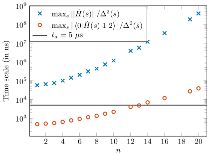
Figure 7: Test of the adiabatic condition. The solid line is the annealing time used in our experiments. Symbols represent the quantity appearing in two versions of the adiabatic condition [for ASC parameters $(1,0.5,175)$] that should be smaller than the annealing time in order for the adiabatic condition to hold.

Appendix E Test of the adiabatic condition

Here we test the validity conditions assumed for the derivation of the adiabatic Markovian master equation Albash et al. (2012), and in particular that the adiabatic approximation is satisfied. To this end we test the ‘folklore’ adiabatic condition $t_{f}\gg\max_{s}|\langle g|\dot{H}(s)|e\rangle|/\Delta^{2}(s)$, where $g$ and $e$ are the ground and first (relevant) excited states, respectively, for ASC parameters $(1,0.5,175)$. The result is shown in Supplementary Fig. 7 (red circles), and it can be seen that the condition is satisfied for $n\leq 14$. The relevant first excited state is the two-fermion state $|1\ 2\rangle$. Also shown is the more conservative condition given in terms of the operator norm (blue crosses). The adiabatic condition with the operator norm is not satisfied for any value of $n$, but it has recently been shown that this condition, which involves an extensively growing operator norm, must be replaced by a condition involving local operators Bachmann et al. (2017).

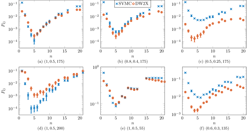
Figure 8: Comparison of the SMVC model to the empirical DW2X results. The error bars everywhere indicate $95\%$ confidence intervals calculated using a binomial bootstrap over the different runs of the simulation. (a) The SVMC parameters were optimized to match the empirical DW2X success probability results for the chain with parameters $(W_{1},W_{2},N)=(1,0.5,175)$. The optimal values found are: $N_{s}=120\times 10^{3},\beta=0.75\text{ (GHz)}^{-1},\sigma=0.05$ [compare to the DW2X’s $t_{f}=5\ \mu\text{s},\beta=0.637\text{ (GHz)}^{-1},\sigma\sim 0.03$]. (b) With the same optimal SVMC parameter values, but with chain parameters $(0.8,0.4,175)$, the SVMC model predicts increased success probability, in contrast to the empirical results. The same trend continues but is more pronounced in (c), with additionally the position of the minimum shifting to the wrong location ($n=7$ vs $n^{*}=4$). Panel (d) shows that increasing the chain length causes a large deviation in the SVMC results [compare to panel (a)], and also shifts the location of the minimum to the wrong value, but (e) shows showing that reducing the chain length does not degrade the agreement much. (f) Results for another chain parameter set, exhibiting a similar discrepancy to that seen in (c).

Chain parameters	DW2X	$k^{*}$	ME	SVMC
$(1.0,0.50,175)$	5,6	5	5,6	5
$(0.5,0.25,175)$	3,4,5	4	4,5	5,6,7
$(0.8,0.40,175)$	5	5	5	5,6
$(1.0,0.50,200)$	5,6	5	5,6	4,5,6
$(1.0,0.50,\phantom{0}55)$	5,6	5	5,6,8	5
$(0.6,0.30,135)$	4,5	4,5	5,6	5,6

Table 2: Locations $n^{*}$ of the DW2X success probability minima vs those found by the fermionic model based on the peak of $k^{*}$, the master equation model (ME), and the SVMC model. When the location of the minimum is ambiguous within our $95\%$ confidence interval we list all values of $n^{*}$ that overlap to within one $\sigma$. The best agreement is obtained by the master equation model.

Appendix F Comparison to the classical SVMC model

The spin vector Monte Carlo (SVMC) model Shin et al. (2014a) was proposed as a purely classical model of the D-Wave processors in response to earlier work that ruled out simulated annealing Boixo et al. (2013) and other work that established a strong correlation between D-Wave ground state success probability data and simulated quantum annealing Boixo et al. (2014). The SVMC model was found to not always correlate well with D-Wave empirical data; for example, deviations were observed for the SVMC model in the case of ground state degeneracy breaking Albash et al. (2015a), excited state distributions Albash et al. (2015b), quantum annealing correction experiments Pudenz et al. (2015) and the dependence of success probability on temperature Boixo et al. (2016). But it has generally been successful in predicting the success probability distributions of D-Wave experiments. The SVMC model thus provides a sensitive test for whether anything other than classical effects are at play in a fixed-temperature measurement of the ground state success probability.

In the SVMC model each qubit is replaced by a classical $O(2)$ rotor parametrized by one continuous angle via $\sigma^{x}_{i}\mapsto\sin\theta_{i}$ and $\sigma^{z}_{i}\mapsto\cos\theta_{i}$, so that the Hamiltonian [Eq. 1] becomes

$$E(s)=-A(s)\sum_{i}\sin\theta_{i}+B(s)\left(-\sum_{i}J_{i}\cos\theta_{i}\cos\theta_{i+1}\right)\ .$$ (56)

In addition, the angles $\theta_{i}$ undergo Metropolis updates every discrete time-step of size $1/N_{s}$, where $N_{s}$ is the number of sweeps, at a fixed inverse temperature $\beta$.

Angle updates are performed as follows. We first divide the dimensionless time $s$ into steps of size $\delta s=1/N_{s}$, where $N_{s}$ is the number of sweeps performed during the course of one run, and initialize to the state $\theta_{i}(s=0)=\pi/2$ for all spins $i$. At each such time step, we pick a random permutation of the set $\{1,2,\ldots,N\}$ where $N$ is the number of qubits in the chain. One by one, we select a random angle for each qubit in this permuted list, changing it from $\theta_{i}$ to $\tilde{\theta}_{i}$ where $\tilde{\theta}_{i}$ is picked randomly from $[0,\pi]$. We calculate the energy change $\Delta E$ for this move and the new angle is accepted with probability

$$p_{i}=\min\left[1,\exp(-\beta\Delta E)\right]\ ,$$ (57)

where $\beta$ is the inverse annealing temperature for the SVMC algorithm. The final state is obtained by projecting the $O(2)$ rotor spins to the computational state at $s=1$, setting spin $i$ to be $1$ ($-1$) if $\cos\theta_{i}>0$ ($<0$). We repeat this process many times in order to estimate the success probability of the algorithm.

In order to realistically emulate the D-Wave processor, we added random Gaussian noise $\mathcal{N}(0,\sigma^{2})$ to each $J_{i}$ Shin et al. (2014b). The SVMC model then has three free parameters: $\{N_{s},\beta,\sigma\}$, which we used to calibrate it against the DW2X data. Toward this end we used the chain with parameters $(1,0.5,175)$ and performed an extensive search in the $\{N_{s},\beta,\sigma\}$ parameter space. As shown in Supplementary Fig. 8(a), we obtain a close match for $N_{s}=120\times 10^{3}$, $\beta=0.75\text{ (GHz)}^{-1}$ and $\sigma=0.05$. This is the best fit we found for this particular chain. In general, we found that the SVMC parameters can be tuned to reproduce the location of the minimum in success probability for any sector size. We were also able to tune the parameters such that the minimum disappears completely and have the success probability increase or decrease monotonically. We were not able to find parameters that give rise to an inverted curve, i.e., a maximum in the success probability. Most of these features can be seen by tuning $\beta$ and keeping the other parameters fixed.

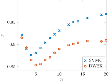
Figure 9: Spin boundary correlation function computed using the SVMC model. The spin boundary correlation function for the same chain and SVMC parameters as in Supplementary Fig. 8(a). The SVMC model does not correctly capture the empirical results despite providing a close match to the success probability in Supplementary Fig. 8(a).

To avoid fine-tuning, we next used the same parameters to compute the success probability of the SVMC model for other chains. As shown in Supplementary Figs. 8(b) and 8(c), the SVMC model has the wrong trend with decreasing $(W_{1},W_{2})$: it exhibits a higher success probability as the coupling energy scale is lowered. The same happens with increased chain length [Supplementary Fig. 8(d)], though to a lesser degree with decreased chain length [Supplementary Fig. 8(e)]. Moreover, as summarized in Table 2, it does not agree as well with the location of the minimum of the success probability as the other models. We emphasize that while we performed an extensive search, we cannot rule out the possibility of another set of parameters (or the inclusion of other parameters) that allow SVMC to reproduce the DW2X results for all chain lengths and energy scales.

As a further test we also considered the spin boundary correlation, defined as the sum of spin correlations over all boundary qubits in the chain, where the boundary qubits are the qubits at the right edge ($r$) of the heavy sector and left edge ($l$) of the light sector:

$$\bar{s}=\frac{1}{|Q|}\sum_{Q}s_{l}s_{r}\ ,$$ (58)

where $Q$ is the set of boundary qubits and $s_{l},s_{r}\in\{0,1\}$. Thus $\bar{s}=1$ represents perfect alignment (a ground state), while $\bar{s}<1$ represents the occurrence of an excited state due to misalignment of the different sectors. Supplementary Fig. 9 shows the results for the same set of optimized parameters that provided strong agreement with the ground state success probability in Supplementary Fig. 8(a). It can be seen that the SVMC model predicts the wrong location for the minimum of $\bar{s}$ and rises too fast. Unfortunately, master equation simulations for $\bar{s}$ are numerically prohibitive, so we cannot assess whether this discrepancy of the SVMC model is fixed by a quantum model.

Appendix G Results at different annealing times

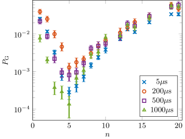
Figure 10: Dependence of the success probability on the annealing times. We show the results for the ASC with parameters $(1.0,0.5,175)$. The error bars everywhere indicate $95\%$ confidence intervals calculated using a bootstrap over different gauges and embeddings. The location of the minimum is unchanged as the annealing time is varied.

In E we discussed the validity of the “folklore” adiabatic condition for the ASC problem. We expect that the adiabatic condition will also be satisfied if we make small changes in the annealing time compared to the vertical scale of Supplementary Fig. 7. Also, neither the gap $\Delta$ nor the number of single fermion states $k^{\ast}$ changes with an increase in the annealing time. Hence we expect that the qualitative nature of the success probability curve, including the location of minima, will be independent of small changes in the annealing time. Since the total thermal transition rate depends on the amount of time system spends near the quantum minimum gap point $s^{\ast}$, we do expect to see changes in the value of the success probability. In Supplementary Fig. 10, we show the change in success probability as we vary the annealing time on the D-Wave device. As expected, the location of the minima remains unchanged. We do find that the success probability varies depending on the annealing time and sector size.