Algorithmic aspects of
$M$-Lipschitz mappings of graphs

Abstract

$M$-Lipschitz mappings of graphs (or equivalently graph-indexed random walks) are a generalization of standard random walk on $\mathbb{Z}$. For $M\in\mathbb{N}$, an $M$-Lipschitz mapping of a connected rooted graph $G=(V,E)$ is a mapping $f:V\to\mathbb{Z}$ such that root is mapped to zero and for every edge $(u,v)\in E$ we have $|f(u)-f(v)|\leq M$.

We study two natural problems regarding graph-indexed random walks.

1. Computing the maximum range of a graph-indexed random walk for a given graph.

2. Deciding if we can extend a partial GI random walk into a full GI random walk for a given graph.

We show that both these problems are polynomial-time solvable and we show efficient algorithms for them. To our best knowledge, this is the first algorithmic treatment of Lipschitz mappings of graphs. Furthermore, our problem of extending partial mappings is connected to the problem of list homomorphism and yields a better run-time complexity for a specific family of its instances.

1 Introduction

Graph-indexed random walks (or also $M$-Lipschitz mapping of graphs) are a generalization of standard random walk on $\mathbb{Z}$. This concept has important connections to statistical physics, namely to gas models and Widom–Rowlinson configurations (as is described by Zhao [23] and Cohen et al. [5]). For a more general treatment of random walks, see [18, 11, 16].

Graph-indexed random walks were thoroughly studied, mainly because of the parameter of the average range, for example in [1, 7, 2, 22, 17]. However, we emphasize that algorithmic aspects of graph-indexed random walks were, by our best knowledge, not studied yet.

Applications and motivation.

We believe that our results can be useful in determining the complexity of computing the average range and in statistical physics.

Results on finding the maximum range provide an easy tool to determine the extremal cases of graphs with regard to the number of $1$-Lipschitz mappings. Furthermore, one can ask if there is some $M$-Lipschitz mapping for a given $M$ and a given graph $G$ with $k\in\mathbb{Z}$ as the image of a vertex in $G$. Results in Section 3 provide a clear positive answer to this. We can check this in linear time.

Results on extending partial Lipschitz mappings are motivated by the following.

• Our algorithms for extending partial Lipschitz mappings provide faster algorithms for particular instances of list homomorphism problem compared to algorithms of Feder and Hell in [8, 9].

• We often deal with incomplete or corrupted data. Finding if some given mapping can be a part of an $M$-Lipschitz mapping can be seen as a quick routine to exclude cases of clearly inconsistent data.

2 Preliminaries

We use the standard notation and definitions as in Diestel’s monograph [6]. Intervals in this paper are closed intervals of integers, if not stated otherwise.

A graph homomorphism between digraphs $G$ and $H$ is a mapping $f:V(G)\to V(H)$ such that for every edge $uv\in E(G)$, $f(u)f(v)\in E(H)$. That means that graph homomorphism is an adjacency-preserving mapping between the vertex sets of two digraphs. The set $I:=\{w\in V(H)\mid\exists v\in V(G):f(v)=w\}$ for a graph homomorphism $f$ is called the homomorphic image of $f$.

For a comprehensive and more complete source on graph homomorphisms, the reader is invited to see [12]. A quick introduction is given in [10] as well.

Definition 1

For $M\in\mathbb{N}$, an $M$-Lipschitz mapping of a connected graph $G=(V,E)$ with root $v_{0}\in V$ is a mapping $f:V\to\mathbb{Z}$ such that $f(v_{0})=0$ and for every edge $(u,v)\in E$ it holds that $|f(u)-f(v)|\leq M$. The set of all $M$-Lipschitz mappings of a graph $G$ is denoted by $\mathcal{L}_{M}(G)$.

We strongly emphasize that we are interested in connected graphs only. Components without the root would also allow infinitely many new $M$-Lipschitz mappings. In case of disconnected graphs we can apply a suitable linear transformation (for example $x\to x+1$) to images of vertices we would get a new $M$-Lipschitz mapping.

The root is just some distinguished vertex of $G$. The reason for having graphs rooted is that we want to have finitely many Lipschitz mappings for a fixed graph $G$. One can reason similarly as in the case of disconnected graphs.

In literature, we will often meet a slightly different definition of $1$-Lipschitz mappings. In it the restriction $|f(u)-f(v)|\leq 1$, for all $uv\in E$, is removed and instead, the restriction $|f(u)-f(v)|=1$, for all $uv\in E$, is added. In [17] authors call these mappings strong Lipschitz mappings. We generalize this in the following definition.

Definition 2

For $M\in\mathbb{N}$, a strong $M$-Lipschitz mapping of a connected graph $G=(V,E)$ with root $v_{0}\in V$ is a mapping $f:V\to\mathbb{Z}$ such that $f(v_{0})=0$ and for every edge $(u,v)\in E$ it holds that $|f(u)-f(v)|=M$. The set of all $M$-Lipschitz mappings of a graph $G$ is denoted by $\mathcal{L}_{\pm M}(G)$.

Note that strong $M$-Lipschitz mappings are a special case of $M$-Lipschitz mappings of graph. We further emphasize the following lemma.

Lemma 1

A graph has a strong $M$-Lipschitz mapping iff it is bipartite.

We now define the main parameters for Lipschitz mapping of graphs.

Definition 3

The range of a Lipschitz mapping $f$ of $G$ is the size of the homomorphic image of $f$. Formally $\mathrm{r}_{G}(f):=\big{|}\{z\in\mathbb{Z}\,|\,z=f(v)\textrm{ for some }v\in V(G)\}\big{|}$.

Definition 4

(Average range) The average range of graph $G$ over all $M$-Lipschitz mappings is defined as

$$\mathrm{\overline{r}}_{M}(G):=\frac{\sum_{f\in\mathcal{L}_{M}(G)}\mathrm{r}(f)}{|\mathcal{L}_{M}(G)|}.$$

We can view this quantity as the expected size of the homomorphic image of an uniformly picked random $M$-Lipschitz mapping of $G$.

Definition 5

(Maximum range) The maximum range over all $M$-Lipschitz mappings of graph $G$ is defined as

$$\mathrm{r}^{\max}_{M}(G)=\max_{f\in\mathcal{L}_{M}(G)}\mathrm{r}(f).$$

Whenever we want to talk about the counterparts of these definitions for strong Lipschitz mappings, we denote it with $\pm$ in subscript. For example, $\mathrm{\overline{r}}_{\pm M}$ is the average range of strong $M$-Lipschitz mapping of graph.

Whenever we write average range or maximum range without saying which $M$-Lipschitz mappings we use, it should be clear from the context what $M$ do we mean.

It is worth noting that for computing the average range and the maximum range, the choice of root does not matter. That is why we often omit the details of picking a root.

Connection to graph homomorphisms.

$M$-Lipschitz mappings map graph vertices to integers. There is a natural bijection between $M$-Lipschitz mappings and graph homomorphisms to a suitable graph associated with $\mathbb{Z}$. Consider a graph $Z_{M}$ with the vertex set $V(Z_{M})=\mathbb{Z}$ and the edge set $E(Z_{M})=\{ij:\left|{i-j}\right|\leq M\}$. Every $M$-Lipschitz mapping corresponds to a graph homomorphism to $Z_{M}$.

We can define a graph $Z_{\pm M}$ analogously for strong mappings. Note that in the case of strong $1$-Lipschitz mappings, we get that they correspond to homomorphisms to a two-way infinite path and in the case of $1$-Lipschitz mappings, we get a correspondence to homomorphisms to a two-way infinite path with loops added to each vertex. See Figure 1 for an example of such homomorphism of $C_{4}$.

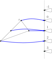
Figure 1: A homomorphism of $C_{4}$ rooted in $r$ to $Z_{1}$ graph. In fact, this homomorphism is a $1$-Lipschitz mapping of $C_{4}$.

Gas models and physical motivation.

A homomorphism from G to $P_{3}$ with loops added to each vertex corresponds to a partial (not necessarily proper) coloring of the vertices of G with red or blue, allowing vertices to be left “uncolored” such that no red vertex is adjacent to a blue vertex. This coloring is known as the Widom–Rowlinson configuration [21] Observe that Widom-Rowlinson configuration corresponds to a $1$-Lipschitz mapping with the size of the homomorphic image at most 3. See Figure 2 for an example.

Widom-Rowlinson configurations have a physical interpretation. Consider particles of a gas $B$ (blue vertices) and of a gas $R$ (red vertices). W-R configurations then model situations in which particles of gases $A$ and $B$ do not interact. This model is sometimes referred to as the hard-core model. The name emphasizes the hard restriction that particles of gases cannot be directly adjacent, i.e. their molecules do not interact.

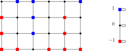
Figure 2: An example of Widom–Rowlinson configuration for a grid graph.

3 Maximum range

In this section we will show how can we algorithmically compute the maximum range of a given graph. Also, we will show the relation of this parameter to other existing results.

3.1 Diameter

In this section we observe one important fact giving us an upper bound on the range of a graph. Then we will show that this upper bound is tight.

We will first prove an important, yet easy lemma.

Lemma 2

For any connected graph $G$ with $\mathrm{diam}(G)$ and every $M$-Lipschitz mapping $f$ of $G$, holds that $\mathrm{r}(f)\leq M\cdot(\mathrm{diam}(G)+1).$

Now we show that we can always construct a mapping where equality holds and thus we conclude that the diameter and the maximum range are tightly connected.

Theorem 3.1

For any connected graph $G$, $\mathrm{r}^{\max}_{M}(G)=M\cdot(\mathrm{diam}(G)+1)$.

Proof

From the definition of the diameter, there must exist vertices $u_{1}$ and $u_{2}$ such that their distance is equal to $\mathrm{diam}(G)$. Without loss of generality we set $r:=u_{1}$. Now let us define the mapping $f:V(G)\to\mathbb{Z}$ so that for every $v\in V$ we have $f(v):=M\cdot d(r,v)$.

We see that $f(r)=0$, and $f(u_{2})=M\cdot d(r,u_{2})$ so the image of the shortest path connecting $u_{1}$ and $u_{2}$ has the size $\mathrm{diam}(G)+1$. On the top of that, for every $uv\in E(G)$, $|f(u)-f(v)|\leq M$, otherwise we would get a contradiction with the definition of the distance. Thus $f$ is an $M$-Lipschitz mapping and its range has to be at least $M\cdot(\mathrm{diam}(G)+1)$. Combining this with Lemma 2, we get the claim weT wanted to prove. ∎

3.2 The case of strong mappings

By Lemma 1 we showed that strong Lipschitz mappings can exist on bipartite graphs only. We will now extend Theorem 3.1.

Theorem 3.2

For any bipartite connected graph $G$, $\mathrm{r}^{\max}_{\pm M}(G)=M\cdot(\mathrm{diam}(G)+1)$.

3.3 Applications

We will apply our results to prove Theorem 3.3 and subsequently to prove extremal behavior on the number of Lipschitz mappings of a graph.

Theorem 3.3

For every connected graph $G=(V,E)$ and for every two vertices $a,b\in V$ such that $ab\not\in E$, holds that

$$\left|{\mathcal{L}_{1}(G)}\right|\geq\left|{\mathcal{L}_{1}(G\cup\{a,b\})}\right|.$$

We will use the Cherry lemma for the proof.

Lemma 3 (Cherry lemma)

A graph $G$ is a disjoint union of complete graphs if and only if it does not contain $K_{1,2}$ as an induced subgraph.

Now we can prove Theorem 3.3.

Proof (Proof of Theorem 3.3)

The graph $G$ cannot be a complete graph. Therefore, by Lemma 3, induced $K_{1,2}$ exists in $G$. Let vertices $a$ and $b$ from the statement of Theorem 3.3 be the two non-adjacent vertices of induced $K_{1,2}$.

We see that $G$ has the diameter at least $2$, since $a$ and $b$ are in distance $2$. Let us root $G$ in $a$ for auxiliary reasons. By the construction of $1$-Lipschitz mapping from Theorem 3.1, there must exist a mapping $f$ with $f(b)=d(a,b)=2$.

Clearly, $\mathcal{L}_{1}(G\cup ab)\subseteq\mathcal{L}_{1}(G)$. However, $f$ cannot be a $1$-Lipschitz mapping of $G\cup ab$ rooted in $a$. That implies $|\mathcal{L}_{1}(G\cup ab)|\leq|\mathcal{L}_{1}(G)|-1$. ∎

Theorem 3.3 further implies the following theorem, giving extremal graphs with respect to the number of Lipschitz mappings.

Corollary 1

Among connected graphs of order $n$, trees have the maximum number of $1$-Lipschitz mappings and a complete graph $K_{n}$ has the minimum number of $1$-Lipschitz mappings.

3.4 Algorithmic aspects

Let us consider the following algorithmic problems – $M$-MaxRange and $M$-Strong-MaxRange.

Problem:	Maximum range problem – $M$-MaxRange
Input:	A connected graph $G$.
Question:	What is the maximum range of $M$-Lipschitz mapping of $G$, i.e. $\mathrm{r}^{\max}_{M}(G)$?

The problem $M$-Strong-MaxRange can be defined similarly.

Because of Theorem 3.1, we can use the existing algorithms for finding graph diameter and distance in graphs for both of these problems. We can achieve an even better complexity for some classes. Take for example the class of trees in which we can compute diameter by a linear-time algorithm using one clever depth-first search traversal.

4 Extending partial Lipschitz mappings

While studying Lipschitz mappings of graphs we came up with an algorithmic problem which falls into widely studied paradigm of a partial structure extension. We give two examples of such problems to show a broader context.

4.1 Related problems

Precoloring extension.

The following problem was introduced in the series of papers [3, 13, 14].

Problem:	Precoloring Extension
Input:	An integer $k\geq 2$, a graph $G=(V,E)$ with $|V|\geq k$, a vertex subset $W\subseteq V$, and a proper $k$-coloring of $G_{W}$.
Question:	Can this $k$-coloring be extended to a proper $k$-coloring of the whole graph $G$?

To current date, more than twenty papers on the precoloring extension problem were published. No up-to-date survey is available, but Daniel Marx gathers an unofficial list of relevant papers on his webpage http://www.cs.bme.hu/~dmarx/prext.php.

The partial representation extension problem.

The reader surely knows a planar drawing of graph. A particular drawing of the underlying graph can be seen as one of the possible representations. Studying the representations of various graph classes is a wide area of graph theory and we refer reader to the comprehensive monograph of Spinrad [19]. One can ask for a given graph $G$ and some partial representation $R^{\prime}$ of $G$ if it can be extended to some full representation $R$ of $G$ such that $R^{\prime}\subseteq R$. This problem was studied for various graph classes, see PhD thesis of Klavík [15] for a survey.

4.2 Definition of our problem

We will define two similar problems in the setting of integer homomorphisms.

Problem:	Partial $M$-Lipschitz mapping extension - $M$-LipExt
Input:	A connected graph $G=(V,E)$, a subset $V^{\prime}\subseteq V$ with a function $f^{\prime}:V^{\prime}\to\mathbb{Z}$.
Question:	Does there exist an $M$-Lipschitz mapping $f$ of $G$ such that $f^{\prime}\subseteq f$?

The problem Strong $M$-LipExt can be defined similarly.

If the answer for a given instance of $M$-LipExt (or Strong $M$-LipExt) is YES, we say that $f^{\prime}$ is extendable for the given $G$ and the given type of problem. We often say only that $f^{\prime}$ is extendable when it is clear from the context which of these two problems we are trying to solve.

See Figure 3 for an initial example. This mapping cannot be extended to a $1$-Lipschitz mapping but it can be extended to an $L$-Lipschitz mapping for every $L\geq 2$.

Figure 3: An example of a partial mapping with three prescribed vertices.

4.3 Partial non-strong $M$-Lipschitz mappings

Polynomiality.

We will show that $M$-ParExt can be polynomially reduced to a tractable instance of list homomorphism problem.

Problem:	List homomorphism problem - LHom($H$)
Input:	A graph $G$ and a list function $L:V(G)\to 2^{V(H)}$.
Question:	Does there exist an homomorphism $f:G\to H$ such that $f(v)\in L(v)$ for every $v\in V(G)$?

Theorem 4.1

The problem $M$-ParExt is polynomial-time solvable.

Proof

(Sketch.) Without loss of generality, assume that $f^{\prime}(V^{\prime})\subseteq[-n,n]$. We define $n:=|V(G)|$. For a given instance of $M$-ParExt instance, build a graph $T$ with $V(T):=\{-n,\ldots,0,\ldots n\}$ and $E(T):=\{(a,b):-n\leq a\leq b\leq n\wedge|a-b|\leq M\}$. If $v\in V^{\prime}$, set $L(v):=\{f^{\prime}(v)\}$ and if $w\in V\setminus V^{\prime}$, set $L(w):=V(T)$. Now observe that answer for LHom($T$) with $G$ on input is positive if and only if $M$-ParExt on $G$ has a positive answer.

Feder and Hell [8] proved that if $H$ has a loop on each vertex and $H$ is an interval graph, then LHom($H$) is tractable. Hence what remains is to prove that $T$ is an interval graph. Our result then follows. ∎

Note that the algorithm in [8] runs in $O(|V|^{4})$ for the case of LHom($Z_{M}$) Our goal in the remaining text will be to show more efficient algorithms for these instances. We note that our approach will be also constructive, as is the algorithm in [8],

Trees.

The goal of this part of the paper is to show that we can solve $M$-ParExt in quadratic time and linear space with a special algorithm. We will now prove the correctness and the complexity of this algorithm.

Algorithm 1 Algorithm for $M$-ParExt on trees.

0:  A tree graph $G$, a vertex set $V^{\prime}\subseteq V(G)$, and a partial $M$-Lipschitz mapping $f^{\prime}:V^{\prime}\to\mathbb{Z}$.

1:  Check if $|f^{\prime}(v)-f^{\prime}(u)|\leq M$ for all $u,v\in V^{\prime}$. If not, $f^{\prime}$ cannot be extended.

2:  Set $P(v):=[f^{\prime}(v),f^{\prime}(v)]$ for every $v\in V^{\prime}$,

3:  Set $P(v):=[-\infty,\infty]$ for every $v\in V(G)\setminus V^{\prime}$.

4:  for every $v^{\prime}$ in $V^{\prime}$ do

5:     Start the DFS on $G$ from $v^{\prime}$.

6:     In DFS, when you process vertex $v$ with $P(v)=[\underline{P}(v),\overline{P}(v)]$, do the following:

7:     for every $w\in N_{G}(v)$ do

8:        $P(w):=[\underline{P}(v)-M,\overline{P}(v)+M]\cap P(w)$.

9:     end for

10:  end for

11:  Find $r\in V(G)$ such that $0\in P(v)$ and re-run DFS from Line 5 with $v^{\prime}=r$.

12:  if no such r exists then

13:     return  The mapping $f^{\prime}$ cannot be extended.

14:  end if

15:  Set $f(r):=0$.

16:  if $P(v)=\emptyset$ for some $v\in V(G)$ then

17:     return  The mapping $f^{\prime}$ cannot be extended.

18:  end if

19:  Launch the BFS from $r$ and for every visited vertex $v\neq r$, set $f(v)$ so that for parent vertex $p$, $f(v)\in[f(p)-M,f(p)+M]$ holds.

20:  if the previous BFS could not be completed then

21:     return  false

22:  end if

23:  return  true

Lemma 4 (Correctness)

Algorithm 1 is correct. It finds an $M$-Lipschitz mapping $f$ that extends $f^{\prime}$ if and only if $f^{\prime}$ is extendable.

Proof

Suppose that the algorithm returns a mapping $f$. We claim that it is an $M$-Lipschitz mapping extending $f^{\prime}$. Obviously, there exists a vertex mapped to zero under $f$ – the vertex $r$. Furthermore, the condition

$$|f(u)-f(v)|\leq M,\forall uv\in E(G)$$

holds, otherwise the algorithm would stop on Line 20. Finally, we observe that for every $v^{\prime}\in V^{\prime}$, interval $P(v^{\prime})$ is equal to $[f^{\prime}(v^{\prime}),f^{\prime}(v^{\prime})]$ at the end of the algorithm so $f$ extends $f^{\prime}$. That finishes the only if part of the equivalence.

Now let us prove the if part. We will prove that if the algorithm does not find an $M$-Lipschitz mapping $f$ extending $f^{\prime}$, then $f^{\prime}$ is not extendable.

Algorithm can stop and fail to find such $f$ exactly from the following reasons:

1. Algorithm could not find a candidate for the root. (Line 12)

   If at the end of the algorithm for every vertex $v\in V$, $0\not\in P(v)$, then for every $v\in V$ exists some vertex $v^{\prime}\in V^{\prime}$ such that $|f(v^{\prime})|>M\cdot d(v,v^{\prime})$. We see that $f^{\prime}$ is not extendable.

2. There exists $v\in V$ such that $P(v)=\emptyset$. (Line 16)

   If such $v$ exists, then it implies the existence of two vertices $c,d\in V^{\prime}$ such that the intersection $I=[f^{\prime}(c)-M\cdot(c,v),f^{\prime}(c)+M\cdot(c,v)]\cap[f^{\prime}(d)-M\cdot(d,v),f^{\prime}(d)+M\cdot(d,v)]$ is empty. However, $I$ is exactly the set of all possible images that we can assign to $v$ if $c$ is set to $f^{\prime}(c)$ and $d$ is set to $f^{\prime}(d)$. We conclude that $f^{\prime}$ is not extendable.

3. Algorithm could not complete the BFS phase. (Line 20)

   We will actually show that this case is not possible since the only possibility how 3) can happen is that some final interval $P(v)$ for some $v\in V$ is empty and the algorithm will halt even before the BFS phase can start (more precisely, the algorithm would already stop at line 16 and the case 2) occurs).

   Assume that all intervals $P(v)$ are nonempty. Consider an edge $xy\in E(G)$. Without loss of generality, in the last DFS phase (Line 11), $x$ was processed before $y$. Consider intervals $P^{\prime}(x),P^{\prime}(y)$ defined as the intervals $P(x),P(y)$, respectively, before the last DFS phase. Clearly, when $x$ was processed in the last DFS phase, $P(y)$ was set to $P^{\prime}(y)\cap[P^{\prime}(x)-M,P^{\prime}(x)+M]$; a nonempty interval and therefore,

   $$\forall i\in P(x),\exists j\in P(y):|i-j|\leq M.$$

   And conversely,

   $$\forall j\in P(y),\exists i\in P(x):|i-j|\leq M.$$

   We conclude that the case 3) cannot occur.

This proves the if part and we are done. ∎

We can now conclude the main theorem for trees.

Theorem 4.2

$M$-ParExt for trees is solvable in time $O(|V|^{2})$ and space $O(|V|)$.

Proof

We proved that Algorithm 1 is correct.

We are running $O(|V|)$ times depth-first search on $G$ plus we perform a constant number of linear traversals of data structure for $G$. That, combined with $G$ being a tree, concludes the claim. ∎

General case.

The goal of this section is to show an efficient constructive algorithm for the general case.

Theorem 4.3

The problem $M$-ParExt is solvable in polynomial time on general graphs. There is an algorithm for it running in time $O(|V|^{3})$ and $O(|V|^{2})$ space. Furthermore, if an instance for $M$-ParExt is rooted, we have an algorithm running in time $O(|V||E|)$ and space $O(|V|^{2})$.

It will be useful to define two new properties for integer functions on vertex sets.

Definition 6 ($M$-reachability)

We call a mapping $f:V^{\prime}\to\mathbb{Z}$ of graph $G$, with $V^{\prime}\subseteq V(G)$, $M$-reachable if every pair of vertices $u,v\in V^{\prime}$ satisfies

$$\left|{f(u)-f(v)}\right|\leq M\cdot d(u,v),$$

We omit for which graph is a mapping $M$-reachable if it clear from context.

Definition 7

We call a mapping $f:V^{\prime}\to\mathbb{Z}$ of graph $G$, with $V^{\prime}\subseteq V(G)$, rooted if $f^{-1}(0)\neq\emptyset$.

We can now state and prove the full characterization of extendable situations.

Theorem 4.4

For a graph $G=(V,E)$, subset $V^{\prime}\subseteq V$, and a partial mapping $f^{\prime}:V^{\prime}\to\mathbb{Z}$, the following statements are equivalent:

1. The mapping $f^{\prime}$ is extendable to a $M$-Lipschitz mapping.

2. One of the following holds:

   1. The mapping $f^{\prime}$ is $M$-reachable and rooted.

   2. There exist $r\in V\setminus V^{\prime}$ with $f^{\prime\prime}$ defined as $f^{\prime\prime}:=f^{\prime}\cup(r,0)$, such that $f^{\prime\prime}$ is $M$-reachable.

Proof

$(1)\implies(2)$: For brevity, we will handle the (a) case, (b) case is similar. Assume that $f^{\prime}$ is extendable to an $M$-Lipschitz mapping $f^{*}$. Choose a pair of vertices $u,v\in V^{\prime}$ such that $\left|{f(u)-f(v)}\right|>M\cdot d(u,v)$. Pick a shortest path $u=x_{1},\ldots,x_{l}=v$ between $u$ and $v$. Each summand of the sum $\sum_{i=2}^{l}(f(x_{i})-f(x_{i-1}))$ is at most $M$ and at least $-M$, which contradicts that the mapping $f^{*}$ is $M$-Lipschitz.

$(2)\implies(1)$: Again, we will only prove the (a) case, (b) can be done in analogous way. We will show that we can extend $f^{\prime}$ mapping by one vertex and preserve $M$-reachability. By applying this inductively we will prove that $(2)$ implies $(1)$.

Choose a vertex $a$ that is adjacent to some vertex $b$ such that $f^{\prime}(b)$ is defined and $f^{\prime}(a)$ is not defined. For every vertex $c\in f^{\prime}(V^{\prime})$, the vertex $b$ is reachable. Thus we can always find a number for $a$ such that $c$ will be reachable from $a$. For every $c$ we can define interval $I_{c}$ containing all possible values for $a$ such that $c$ is reachable from $a$. This is a closed connected interval in $\mathbb{Z}$. Furthermore, the set system $\{I_{c}|\forall c\in f^{\prime}(V^{\prime})\}$ has the Helly property. Finally, for every two $c_{1},c_{2}\in f^{\prime}(V^{\prime})$ there is a nonempty intersection. Otherwise we would get contradiction with $M$-reachability of $f^{\prime}$. Thus we can pick a suitable $k\in\Large\cap_{c\in f^{\prime}(V^{\prime})}I_{c}$ and extend $f^{\prime}$ by setting $f^{\prime}:=f^{\prime}\cup\{(a,k)\}$. We also set $V^{\prime}:=V^{\prime}\cup a$. ∎

Theorem 4.4 and its proof yield an algorithm for constructing an extended mapping. Now we can finally prove Theorem 4.3.

Algorithm 2 A constructive algorithm for $M$-ParExt on general graphs.

0:  A graph $G$, a set of vertices $V^{\prime}\subseteq V(G)$, and a partial $M$-Lipschitz mapping $f^{\prime}:V^{\prime}\to\mathbb{Z}$.

1:  Compute all-pairs distances using Thorup’s algorithm [20].

2:  if $f^{\prime}$ rooted then

3:     Set $f^{\prime\prime}:=f^{\prime}$ and go to line 8.

4:  end if

5:  if $f^{\prime}$ not rooted then

6:     for every $v^{\prime}$ in $V\setminus V^{\prime}$ do

7:        Set $f^{\prime\prime}:=f^{\prime}\cup(v^{\prime},0)$.

8:        if $f^{\prime\prime}$ is $M$-reachable then

9:           while some vertex not mapped under $f^{\prime\prime}$ do

10:              Pick a non-mapped vertex $a$ adjacent to some already mapped vertex.

11:              Choose some $k\in\Large\cap_{c\in f^{\prime\prime}(V^{\prime\prime})}I_{c}$ with $c$’s nad $I_{c}$’s defined analogously as in the proof of Theorem 4.4.

12:              Set $f^{\prime\prime}:=f^{\prime\prime}\cup(a,k)$.

13:           end while

14:           return  true

15:        else

16:           return  false

17:        end if

18:     end for

19:  end if

Proof (Proof of Theorem 4.3)

Because of Theorem 4.4 our Algorithm 2 is correct. We need to analyze its complexity.

Line 1 computes all-pairs distances in time $O(|V||E|)$. Line 8 takes $O(|V|^{2})$ time and the code between lines 10 and 12 also. If $f^{\prime}$ was rooted, we jump straight into the for-cycle and thus $O(|V|)$ factor is saved, otherwise we get additional factor $O(|V|)$. Thus we conclude the claim. ∎

Fixed range and the maximum possible range.

We can also ask if it is possible to extend a given mapping to an $M$-Lipschitz mapping with a given range. Naturally, one can also define MaxRange-$M$-LipExt asking for the maximum possible range of extending mapping. Minimum variant can be approached in the same manner. Formally, we have the following problem.

Problem:	Partial $M$-Lipschitz mapping extension with a fixed range - FixedRange-$M$-LipExt
Input:	A connected graph $G=(V,E)$, a subset $V^{\prime}\subseteq V$ with a function $f^{\prime}:V^{\prime}\to\mathbb{Z}$ and $r\in\mathbb{N}$.
Question:	Does there exist an $M$-Lipschitz mapping $f$ of $G$ such that $f^{\prime}\subseteq f$ and $\mathrm{r}(f)=r$?

Using Algorithm 2 as a subroutine we can first choose an interval $[a,b]$ such that $a,b\in\mathbb{N}$ and $0\in[a,b]$. Then we can choose independently two different vertices $v_{a},v_{b}\in V\setminus V^{\prime}$ . We can then set $f_{[a,b],v_{a},v_{b}}:=f^{\prime}\cup(v_{b},b)\cup(v_{a},a)$. Of course, $a$ (or $b$) can already be the image of some vertex in $V^{\prime}$ and in that case we choose only $v_{b}$ (or $v_{a}$).

For every choice of $[a,b]$ and $v_{a},v_{b}$ we run Algorithm 2 and see if $f_{[a,b],v_{a},v_{b}}$ can be extended. This algorithm is correct and since $\left|{a-b}\right|\leq|V|$ we deduce that FixedRange-$M$-LipExt can be solved in time $O(|V|^{7})$. Furthermore, MaxRange-$M$-LipExt can be solved in time $O(|V|^{7}\cdot\log|V|)$ by combining the algorithm for FixedRange-$M$-LipExt with a binary search for a suitable $r$.

Finally, we note that in the case of diameter being bounded we can easily modify these algorithms to run in time $O(|V|^{5})$ for both FixedRange-$M$-LipExt and MaxRange-$M$-LipExt.

4.4 Partial strong $M$-Lipschitz mappings

We note that for Strong $M$-LipExt we can modify Algorithm 1 and 2. However, more involved analysis is needed. If we are satisfied with a worse running time, we can conclude the following theorem by analysis similar to that for $M$-LipExt in Theorem 4.1, using results of Feder and Hell [9].

Theorem 4.5

Strong $M$-LipExt is solvable in polynomial time.

5 Concluding remarks

We initiated the study of algorithmic aspects of Lipschitz mappings of graphs. We showed that the problem of finding the maximum range and extending partial Lipschitz mapping are both solvable in polynomial time.

We conclude with two open problems stemming from our research.

Improving the complexity of extension problems.

The following open problem naturally arises: Are there algorithms for FixedRange-$M$-LipExt and MaxRange-$M$-LipExt running in time asymptotically better than ours?

Average range.

We propose to settle the complexity of the following natural problem associated with the average range. The problem $M$-AvgRange has a connected graph $G$ on input. We ask what is the average range of $M$-Lipschitz mappings of $G$, i.e. $\mathrm{\overline{r}}_{M}(G)$? Even the case $M=1$ seems challenging.

We note that for several classes of graphs, e.g. paths, cycles, complete graphs, complete bipartite graphs we showed [4] a closed formulas implying that we can compute $1$-AvgRange for these classes efficiently.

Appendix 0.A Omitted theorems and proofs

Proof

(of Lemma 1) Observe that in every strong $M$-Lipschitz mapping, all vertices are mapped to some number of the form $k\cdot M$, where $k\in\mathbb{Z}$.

Consider a non-bipartite graph $G$ and a strong $M$-Lipschitz mapping $f$ of $G$. We recall that a graph is bipartite if and only if it does not contain a cycle of odd length as a subgraph.

Therefore, $G$ contains some odd cycle $C$ with edges $v_{1}v_{2},\ldots,v_{l}v_{1}$. Let us denote

$$e_{i}:=f(v_{(i+1\textrm{ mod }l)})-f(v_{(i\textrm{ mod }l)}),\forall i\in\{1,\ldots,n\}.$$

We see that $e_{i}\in\{+M,-M\}$. Moreover, $\sum_{i=0}^{n}e_{i}=0$ from the definition of $e_{i}$. However, this sum has an odd number of summands and thus we get a contradiction. ∎

Proof

(of Lemma 2) The existence of $f$ with $\mathrm{r}(f)>M\cdot(\mathrm{diam}(G)+1)$ would imply the existence of a path subgraph in $G$ with endpoints $u,v$ such that their images would be in distance $|f(u)-f(v)|=M\cdot(\mathrm{diam}(G)+1)$. However, that would mean that all paths between $u$ and $v$ have to map to some connected subgraph of $\mathbb{Z}$ of size greater than $M\cdot(\mathrm{diam}(G)+1)$ which is a contradiction with the definition of diameter. ∎

Proof

(of Theorem 3.2) We can take Lipschitz mapping $f$ as in Theorem 3.1. However, we have to check if it is a strong $M$-Lipschitz mapping.

Suppose that $f$ is not a strong $M$-Lipschitz mapping. That means that there exist two vertices $a,b\in V(G)$ such that $ab\in E(G)$ and $f(a)=f(b)$. Furthermore, from the definition of $f$, $d(r,a)=d(r,b)$. Define $l:=d(r,a)$.

From the definition of the distance, we get that there exist an $(r,a)$-path and $(r,b)$-path, both of length $l$. Since $G$ is bipartite, parts to which vertices belong have to alternate along the $(r,a)$-path and along the $(r,b)$-path as well. Additionally, parts to which $a$ and $b$ belong are determined by the parity of their distance from root. But that means that $a$ and $b$ belong to the same part. Since they are neighbors, we get a contradiction.

Finally, we note that the previous argument works also in the case of $r$ being either the vertex $a$ or $b$. ∎

References

- [1] Itai Benjamini, Olle Häggström, and Elchanan Mossel. On random graph homomorphisms into Z. Journal of Combinatorial Theory, Series B, 78(1):86–114, 2000.
- [2] Itai Benjamini and Gideon Schechtman. Upper bounds on the height difference of the Gaussian random field and the range of random graph homomorphisms into Z. Random Structures and Algorithms, 17(1):20–25, 2000.
- [3] Miklós Biro, Mihály Hujter, and Zsolt Tuza. Precoloring extension I: Interval graphs. Discrete Mathematics, 100(1-3):267–279, 1992.
- [4] Jan Bok. Graph-indexed random walks on special classes of graphs. arXiv preprint arXiv:1801.05498, 2018.
- [5] Emma Cohen, Will Perkins, and Prasad Tetali. On the Widom–Rowlinson occupancy fraction in regular graphs. Combinatorics, Probability and Computing, 26(2):183–194, 2017.
- [6] Reinhard Diestel. Graph theory Graduate texts in mathematics; 173. Springer-Verlag Berlin and Heidelberg GmbH, 2000.
- [7] Anna Erschler. Random mappings of scaled graphs. Probability theory and related fields, 144(3-4):543–579, 2009.
- [8] Tomas Feder and Pavol Hell. List homomorphisms to reflexive graphs. Journal of Combinatorial Theory, Series B, 72(2):236–250, 1998.
- [9] Tomas Feder, Pavol Hell, and Jing Huang. List homomorphisms and circular arc graphs. Combinatorica, 19(4):487–505, 1999.
- [10] Chris Godsil and Gordon F Royle. Algebraic graph theory, volume 207. Springer Science & Business Media, 2013.
- [11] Olle Häggström. Finite Markov chains and algorithmic applications, volume 52. Cambridge University Press, 2002.
- [12] Pavol Hell and Jaroslav Nešetřil. Graphs and homomorphisms. Oxford Lecture Series in Mathematics and its Applications, 2004.
- [13] Mihály Hujter and Zsolt Tuza. Precoloring extension II: Graph classes related to bipartite graphs. Acta Mathematica Universitatis Comenianae, 62(1):1–11, 1993.
- [14] Mihály Hujter and Zsolt Tuza. Precoloring extension III: Classes of perfect graphs. Combinatorics, Probability and Computing, 5(1):35–56, 1996.
- [15] Pavel Klavík. Extension Properties of Graphs and Structures. Charles University, 2017.
- [16] Gregory F Lawler and Vlada Limic. Random walk: a modern introduction, volume 123. Cambridge University Press, 2010.
- [17] Martin Loebl, Jaroslav Nešetřil, and Bruce Reed. A note on random homomorphism from arbitrary graphs to Z. Discrete mathematics, 273(1):173–181, 2003.
- [18] László Lovász. Random walks on graphs. Combinatorics, Paul Erdos is eighty, 2:1–46, 1993.
- [19] Jeremy P Spinrad. Efficient graph representations. American Mathematical Society, 2003.
- [20] Mikkel Thorup. Undirected single-source shortest paths with positive integer weights in linear time. J. ACM, 46(3):362–394, May 1999.
- [21] Benjamin Widom and John S Rowlinson. New model for the study of liquid–vapor phase transitions. The Journal of Chemical Physics, 52(4):1670–1684, 1970.
- [22] Yaokun Wu, Zeying Xu, and Yinfeng Zhu. Average range of Lipschitz functions on trees. Moscow Journal of Combinatorics and Number Theory, 1(6):96–116, 2016.
- [23] Yufei Zhao. Extremal regular graphs: independent sets and graph homomorphisms. American Mathematical Monthly, 124(9):827–843, 2017.