BFKL and Sudakov Resummation in Higgs Boson Plus Jet Production with Large Rapidity Separation

Abstract

We investigate the QCD resummation for the Higgs boson plus a high $P_{T}$ jet production with large rapidity separations in proton-proton collisions at the LHC. The relevant Balitsky-Fadin-Kuraev-Lipatov (BFKL) and Sudakov logs are identified and resummed. In particular, we apply recent developments of the transverse momentum dependent factorization formalism in the impact factors, which provides a systematic framework to incorporate both the BFKL and Sudakov resummations.

Introduction. The production of a Higgs boson in association with a large transverse momentum jet is an important channel at the LHC to investigate the Higgs boson property, in particular, when they are produced with large rapidity separation Aad:2012tfa ; Chatrchyan:2012ufa ; Dittmaier:2012vm . To explore the full potential to distinguish between different production mechanisms, we need to improve the theoretical computations of this process. There have been great progresses in higher order perturbative calculations in the last few years with next-to-next-to-leading order results available Chen:2014gva ; Boughezal:2015dra ; Boughezal:2015aha ; Caola:2015wna ; Chen:2016zka . In addition, there exist large logarithms to be resummed to all orders to make reliable theoretical predictions. Because of the large rapidity separation between the two final state particles, an important contribution comes from the so-called Balitsky-Fadin-Kuraev-Lipatov (BFKL) evolution Balitsky:1978ic , similar to the Mueller-Navelet (MN) dijet production Mueller:1986ey . Meanwhile, there are Sudakov-type of large logarithms Sudakov:1954sw ; Collins:1984kg , which has been shown in Ref. Sun:2014lna for central rapidity Higgs boson plus jet production. In this paper, we will develop a systematic framework to implement both BFKL and Sudakov resummations for the Higgs boson plus jet production with large rapidity separation at the LHC. This is crucial for phenomenological study to investigate the coupling between the Higgs boson and other particles in the Standard Model.

We focus on the QCD process contributions to the Higgs boson plus jet production ,

$$p(P_{A})+p(P_{B})\to H(y_{1},k_{1\perp})+Jet(y_{2},k_{2\perp})\ ,$$ (1)

where the incoming hadrons carry momenta $P_{A}$ and $P_{B}$, two final state particles with rapidities $y_{1}$ and $y_{2}$, transverse momenta $k_{1\perp}$ and $k_{2\perp}$, respectively. We take the limit of large rapidity difference $Y=|y_{1}-y_{2}|\sim\frac{1}{\alpha_{s}}\gg 1$ , where as schematically shown in Fig. 1, we can write down the following factorization formula in the momentum space as follows

$$\frac{d^{6}\sigma(pp\to H+J)}{dy_{1}dy_{2}d^{2}k_{1\perp}d^{2}k_{2\perp}}=\sum_{b=q,g}\int d^{2}q_{1\perp}d^{2}q_{2\perp}V_{h}(x_{1},q_{1\perp},k_{1\perp})V_{b}(x_{2},q_{2\perp},k_{2\perp})f_{BFKL}(q_{1\perp},q_{2\perp};Y)\ ,$$ (2)

where $V_{b}$ is the impact factor for parton $b$ (quark or gluon), $V_{h}$ for the Higgs boson, and $f_{BFKL}$ represents the BFKL evolution effects due to gluon radiation in the rapidity interval of $Y$. This factorization is very much similar to the MN-dijet production process Mueller:1986ey , where the dijet are well separated in rapidity. There have been great progresses in theory developments for MN-dijet productions Fadin:1998py ; Ciafaloni:1998kx ; Ciafaloni:1998hu ; Bartels:2001ge ; Bartels:2002yj ; Colferai:2010wu ; Caporale:2011cc ; Ducloue:2013hia ; Ducloue:2013bva ; Caporale:2014gpa , and the first detailed experiment measurement have been performed by the CMS collaboration at the LHC Khachatryan:2016udy . The experimental results have been interpreted as an evidence for the BFKL dynamics Ducloue:2013bva . In our previous publication, we have shown that there exist Sudakov logarithms in MN-dijet productions and these logarithms should be resummed as well Mueller:2015ael . Our results in the following can be applied to MN-dijet processes, and will confirm the factorization formula postulated there. The important difference between the Higgs+Jet process and the MN dijet process is that the Higgs mass can serve as an additional scale which makes the Sudakov resummation a bit more non-trivial. Using the Fourier transform, it is straightforward to write the above factorization formula in the coordinate space, where the resummation is performed

$$\frac{d^{6}\sigma(pp\to H+J)}{dy_{1}dy_{2}d^{2}k_{1\perp}d^{2}k_{2\perp}} = \sum_{b}\int\frac{d^{2}b_{1\perp}d^{2}b_{2\perp}}{(2\pi)^{4}}e^{ik_{1\perp}\cdot b_{1\perp}+ik_{2\perp}\cdot b_{2\perp}}$$ (3)

$$\times\widetilde{V}_{h}(x_{1},b_{1\perp},k_{1\perp})\widetilde{V}_{b}(x_{2},b_{2\perp},k_{2\perp})\widetilde{f}_{BFKL}(b_{1\perp},b_{2\perp};Y)\ .$$

It is well-known that both the Sudakov resummation and BFKL evolution can be more conveniently carried out in the coordinate space.

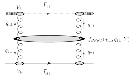
Figure 1: Schematic factorization for Higgs boson and a hard jet production with large rapidity separation between them at the LHC: $f_{BFKL}$ represents the BFKL evolution with gluon radiation in the rapidity interval between the two final state particles; $V_{h}$ and $V_{b}$ for the transverse momentum resummation effects with gluon radiation in the forward rapidity region of the incoming gluon and partons, respectively.

In the inclusive production process, the impact factors can be calculated in the collinear factorization approach. However, in the study of the azimuthal angular distribution between the two final state particles, there exist Sudakov double logarithms in the back-to-back correlation kinematics, where, for example, $k_{1\perp}$ is close to $q_{1\perp}$. To resum these large Sudakov type logarithms, we apply the transverse momentum dependent (TMD) factorization Collins:1984kg ; Collins:2011zzd ; Ji:2004wu for the impact factors in Eq. (2): $V_{h}$ is the TMD gluon distribution, and $V_{b}$ is factorized into the TMD parton distribution and the soft factor associated with the final state jet. The resummation is carried out by solving the relevant evolution equation.

The physical argument for the above factorization is that the higher order gluon radiations can be classified according to the relevant phase space. The most important gluon radiation comes from the large rapidity separation region between the two final state particles, which generates the BFKL evolution effects and can be factorized into the factor $f_{BFKL}$. In the meantime, the gluon radiations in the forward regions of the incoming quark and gluon are factorized into the TMD parton distributions, with a manifest rapidity cut-off in their definitions Collins:2011zzd . Therefore, the BFKL and Sudakov contributions are clearly separated out in the gluon radiation phase space and the factorization can be proved accordingly. This will build a systematic framework to implement both BFKL and Sudakov resummation in the process of Eq. (1).

From the resummation point of view, there are two interesting types of logarithms arising from a one-loop calculation for this process, namely, the BFKL type logarithm $\alpha_{s}Y$ and the Sudakov logarithms. They can be resummed into the factor $f_{BFKL}$ and the impact factors, respectively. As far as the collinear logarithms are concerned, they can be easily dealt with the help of the jet definition and the collinear parton distributions.

The rest of the paper is organized as follows. We take the example of the quark impact factor to demonstrate how the TMD factorization and resummation are applied. Similar results can be obtained for the gluon impact factor. We then calculate the Higgs impact factor, which is factorized into the TMD gluon distribution. Finally, we summarize our results.

Impact Factors for the Quark and Gluon. The partonic scattering of the process described in Eq. (1) comes from quark-gluon and gluon-gluon channels. According to the proposed BFKL factorization, we can separate the calculations into the quark or gluon impact factor and the gluon-Higgs impact factor. Let us take the quark impact factor as an example. At one-loop order, there are virtual and real gluon radiation contributions. The virtual contribution can be written as

$$\Gamma^{v}=\frac{\alpha_{s}}{2\pi}\left(\frac{\mu^{2}}{\vec{q}_{\perp}^{2}}\right)^{\epsilon}\left\{C_{F}\left[-\frac{2}{\epsilon^{2}}-\frac{3}{\epsilon}-\frac{23}{4}+\frac{3}{2}\pi^{2}\right]+{\cal K}\right\}\ ,$$ (4)

where ${\cal K}=C_{A}\left(\frac{67}{18}-\frac{\pi^{2}}{6}\right)-\frac{5}{9}N_{f}$, $C_{F}=4/3$ and $N_{c}=3$, $N_{f}$ represents the number of quark flavors. Here we work in the dimensional regulation with $D=4-2\epsilon$ and $\overline{\textrm{MS}}$ scheme. In the above equation, $\vec{q}_{\perp}$ is the t-channel momentum transfer due to the BFKL factor, and a universal energy dependent term proportional to $C_{A}\ln(s_{0}/\vec{q}_{\perp}^{2})/\epsilon$ is omitted. Together with the similar term from the real gluon radiation, it generates the corresponding BFKL contribution, which can be used to derive the well-known BFKL evolution equation. The detailed procedure can be found in Ref. Mueller:2015ael ; Watanabe:2016gws . In the following, we will focus on the QCD dynamics associated with the Sudakov logarithms, and neglect the BFKL part to simplify the derivations. The real gluon radiation amplitude has also been calculated,

$$\frac{\alpha_{s}}{2\pi^{2}}\int d^{2}k_{\perp}\left[\frac{1+z^{2}}{1-z}-\epsilon(1-z)\right]\left\{C_{F}\frac{(1-z)^{2}q_{\perp}^{2}}{k_{\perp}^{2}(k_{\perp}-(1-z)q_{\perp})^{2}}\right\}\ ,$$ (5)

where $(1-z)$ is the momentum fraction of the incoming quark carried by the radiated gluon with transverse momentum $k_{\perp}$. Clearly, there are two important contributions from the singularities in the above equation: (1) collinear gluon radiation associated with the incoming quark when $k_{\perp}\to 0$; (2) soft gluon radiation associated with the final state jet when $k_{\perp}\sim(1-z)q_{\perp}$. We take the leading power contribution in the limit of $k_{\perp}\ll q_{\perp}$, where soft gluon radiation with $z\to 1$ plays an important role. By apply the plus function prescription to separate out the collinear gluon radiation from the incoming quark, we are left with the following term,

$$\frac{\alpha_{s}}{2\pi^{2}}C_{F}\frac{1}{k_{\perp}^{2}}\delta(1-z)\int\frac{d\alpha}{\alpha}(1+(1-\alpha)^{2})\frac{\alpha^{2}q_{\perp}^{2}}{(k_{\perp}-\alpha q_{\perp})^{2}}\ ,$$ (6)

which contains the collinear divergence associated with the final state jet. Following the same procedure described in Refs. Mueller:2013wwa ; Sun:2014gfa ; Sun:2015doa , we apply the anti-$k_{t}$ jet algorithm and the narrow jet approximation Jager:2004jh ; Mukherjee:2012uz which lead to

$$\frac{\alpha_{s}}{2\pi^{2}}\frac{1}{k_{\perp}^{2}}\left[\ln\frac{q_{\perp}^{2}}{k_{\perp}^{2}}+\ln\frac{1}{R^{2}}+\epsilon\left(\frac{1}{2}\ln^{2}\frac{1}{R^{2}}+\frac{\pi^{2}}{6}\right)\right]\ ,$$ (7)

where $R$ represents the jet size. The soft divergence in the above equation will be cancelled out by the virtual contribution in Eq. (4). To see this more clearly, we introduce the Fourier transform in $b_{\perp}$-space: $V_{q}(x,k_{1\perp},q_{1\perp})=\int\frac{d^{2}b_{\perp}}{(2\pi)^{2}}e^{i(k_{1\perp}-q_{1\perp})\cdot b_{\perp}}\widetilde{V}_{q}(x,b_{\perp})$, and write the one-loop result for $\widetilde{V}_{q}$ as

$$\widetilde{V}_{q}^{(1)}(b_{\perp}) = \widetilde{V}_{q}^{(0)}(b_{\perp})\frac{\alpha_{s}}{2\pi}\left\{C_{F}{\cal P}_{qq}(z)\left(-\frac{1}{\epsilon}-\ln\frac{q_{\perp}^{2}b_{\perp}^{2}}{c_{0}^{2}}\right)-(1-z)C_{F}\right.$$ (9)

$$\left.+\delta(1-z)\left[C_{F}\left(-\frac{1}{2}\ln^{2}\left(\frac{q_{\perp}^{2}b_{\perp}^{2}}{c_{0}^{2}}\right)+\left(\frac{3}{2}-\ln\frac{1}{R^{2}}\right)\ln\frac{q_{\perp}^{2}b_{\perp}^{2}}{c_{0}^{2}}\right)+{\cal K}+\Delta I_{q}\right]\right\}\ ,$$

where $\widetilde{V}_{q}^{(0)}$ represents the leading order normalization, $c_{0}=2e^{-\gamma_{E}}$, ${\cal P}_{qq}(z)$ is the quark-quark splitting kernel and $\Delta I_{q}=C_{F}\left[\frac{3}{2}\ln\frac{1}{R^{2}}+\frac{3}{4}+\frac{2}{3}\pi^{2}\right]$. In reaching the above expression, we have also included the jet contribution Sun:2015doa . Clearly, there are Sudakov double and single logarithms. The above result can be factorized into the TMD quark distribution and the soft factor associated with the final state jet. Here we follow the Collins 2011 scheme for the definition of TMDs, which are defined with soft factor subtraction Collins:2011zzd as follows

$$f_{q}^{(sub.)}(x,b_{\perp},\mu_{F},\zeta_{c})=f_{q}^{unsub.}(x,b_{\perp})\sqrt{\frac{S_{2}^{\bar{n},v}(b_{\perp})}{S_{2}^{n,\bar{n}}(b_{\perp})S_{2}^{n,v}(b_{\perp})}}\ ,$$ (10)

where $b_{\perp}$ is the Fourier conjugate variable respect to the transverse momentum $k_{\perp}$, $\mu_{F}$ the factorization scale and $\zeta_{c}^{2}=x^{2}(2v\cdot P)^{2}/v^{2}=2(xP^{+})^{2}e^{-2y_{n}}$ with $y_{n}$ the rapidity cut-off in the Collins-2011 scheme. The second factor corresponds to the soft factor subtraction with $n$ and $\bar{n}$ as the light-front vectors $n=(1^{-},0^{+},0_{\perp})$, $\bar{n}=(0^{-},1^{+},0_{\perp})$, whereas $v$ is an off-light-front four-vector $v=(v^{-},v^{+},0_{\perp})$ with $v^{-}\gg v^{+}$. The un-subtracted TMD reads as

$$f_{q}^{unsub.}(x,k_{\perp}) = \frac{1}{2}\int\frac{d\xi^{-}d^{2}\xi_{\perp}}{(2\pi)^{3}}e^{-ix\xi^{-}P^{+}+i\vec{\xi}_{\perp}\cdot\vec{k}_{\perp}}\left\langle PS\left|\overline{\psi}(\xi){\cal L}_{n}^{\dagger}(\xi)\gamma^{+}{\cal L}_{n}(0)\psi(0)\right|PS\right\rangle\ ,$$ (11)

with the gauge link defined as ${\cal L}_{n}(\xi)\equiv\exp\left(-ig\int^{-\infty}_{0}d\lambda\,v\cdot A(\lambda n+\xi)\right)$. The light-cone singularity in the un-subtracted TMDs is cancelled out by the soft factor as in Eq. (10) with $S^{v_{1},v_{2}}$ defined as

$$S_{2}^{v_{1},v_{2}}(b_{\perp})={\langle 0|{\cal L}_{v_{2}}^{\dagger}(b_{\perp}){\cal L}_{v_{1}}^{\dagger}(b_{\perp}){\cal L}_{v_{1}}(0){\cal L}_{v_{2}}(0)|0\rangle}\,.$$ (12)

Following the similar idea, we introduce a subtracted soft factor associated with the final state jet,

$$S_{J}(b_{\perp},\mu_{F})=\sqrt{\frac{S_{n,n_{1}}(b_{\perp})S_{n_{1},\bar{n}}(b_{\perp})}{S_{n,\bar{n}}(b_{\perp})}}\ ,$$ (13)

where $n_{1}$ represents the jet direction. One-loop calculation leads to the following result,

$$S_{J}^{(1)}=\frac{\alpha_{s}}{2\pi}C_{F}\left[\ln\frac{1}{R^{2}}\ln\frac{b_{\perp}^{2}\mu_{F}^{2}}{c_{0}^{2}}+\frac{1}{2}\ln^{2}\left(\frac{1}{R^{2}}\right)+\frac{\pi^{2}}{6}\right]\ ,$$ (14)

again with narrow jet approximation, from which we obtain the anamolous dimension $\gamma^{(s)}=\frac{\alpha_{s}}{2\pi}C_{F}\ln(1/R^{2})$. Together with the result for the quark distribution from Ref. Collins:2011zzd ; Sun:2013hua , the following TMD factorization can be verified at one-loop order,

$$\widetilde{V}_{q}(x,b_{\perp})=f_{q}^{(sub.)}(x,b_{\perp},\mu_{F},\zeta_{c})S_{J}(b_{\perp},\mu_{F})H(q_{1\perp},\mu_{F})\ .$$ (15)

Furthermore, in order to eliminate the large logarithms in the hard factor $H^{(1)}$, we have to choose the appropriate scales as $\mu_{F}^{2}=\zeta_{c}^{2}=\vec{q}_{\perp}^{2}$. This corresponds to the factorization that the TMD quark distribution only contains contribution from the gluon radiation in the forward region of the incoming quark. The gluon radiation in the central region (rapidity interval between the two final state particles) belongs to the BFKL evolution. Finally, following the Collins-Soper-Sterman (CSS) resummation approach Collins:1984kg , we obtain the all order result as follows

$$\widetilde{V}_{q}(x,b_{\perp}) = \widetilde{V}_{q}^{(0)}e^{-S_{q}(q_{\perp},b_{\perp})}C\otimes f_{q}(x,\bar{\mu}={c_{0}}/{b})\left[1+\frac{\alpha_{s}}{2\pi}\left({\cal K}+\Delta I_{q}\right)\right]\ ,$$ (16)

where $\otimes$ represents the convolution in $x$ and $f_{q}(x,\bar{\mu})$ the integrated quark distribution. Following the so-called “TMD” scheme Catani:2000vq ; Prokudin:2015ysa in CSS resummation, the hard and soft factors at the appropriate scale lead to the coefficients at $\alpha_{s}$, represented by ${\cal K}$ and $\Delta I_{q}$. The Sudakov factor can be written as

$$S_{q}(q_{\perp},b_{\perp})=\int_{c_{0}^{2}/b_{\perp}^{2}}^{q_{\perp}^{2}}\frac{d\mu^{2}}{\mu^{2}}\left[A_{q}\ln\frac{q_{\perp}^{2}}{\mu^{2}}+B_{q}+D_{q}\ln\frac{1}{R^{2}}\right]\ ,$$ (17)

with $A_{q}=\sum_{i}A_{q}^{(i)}$, $A_{q}^{(1)}=D_{q}^{(1)}=\frac{\alpha_{s}}{2\pi}C_{F}$, $B_{q}^{(1)}=-\frac{3}{2}A_{q}^{(1)}$, and the $C$ coefficient function is $C^{(1)}=\frac{\alpha_{s}}{2\pi}C_{F}(1-x)$.

Similar calculations can be performed for the gluon impact factor,

$$\widetilde{V}_{g}(x,b_{\perp}) = \widetilde{V}_{g}^{(0)}e^{-S_{g}(q_{\perp},b_{\perp})}C\otimes f_{g}(x,\bar{\mu}={c_{0}}/{b})\left[1+\frac{\alpha_{s}}{2\pi}\left({\cal K}+\Delta I_{g}\right)\right]\ ,$$ (18)

with one-loop results as $A_{g}^{(1)}=D_{g}^{(1)}=\frac{\alpha_{s}}{2\pi}C_{A}$, $B_{g}^{(1)}=-2\beta_{0}A^{(1)}$. and $\Delta I_{g}=C_{A}\left(2\beta_{0}\ln\frac{1}{R^{2}}-\frac{\pi^{2}}{6}\right)-\frac{N_{f}}{6}$ with $\beta_{0}=\frac{11}{12}-\frac{N_{f}}{18}$ and $N_{f}$ being the number of flavors. The $C$ coefficient vanishes at one-loop order. In the BFKL factorization, the quark and gluon impact factors are universal, which means that they are same as those in MN-dijet processes. Indeed, we can apply the above impact factors and obtain the consistent results as those in Ref. Mueller:2015ael .

Impact Factor for the Higgs Boson. The computation procedure of the last section can be applied to the Higgs impact factor as well. At the one-loop order, the virtual graph contribution in the gluon-to-Higgs boson impact factor can be deduced from that in Higgs boson plus jet production by taking the limit of the large rapidity separation between the final state particles Ravindran:2002dc ; Glosser:2002gm ,

$$\Gamma^{v}=\frac{\alpha_{s}}{2\pi}\left(\frac{\mu^{2}}{\vec{q}_{\perp}^{2}}\right)^{\epsilon}\left\{N_{c}\left[-\frac{1}{\epsilon^{2}}+\frac{1}{\epsilon}\left(\ln\frac{\tilde{m}^{2}}{\vec{q}_{\perp}^{2}}-2\beta_{0}\right)\right]+\Delta I_{h}+{\cal K}\right\}\ ,$$ (19)

where $\tilde{m}^{2}=m_{h}^{2}+\vec{q}_{\perp}^{2}$ with Higgs mass $m_{h}$, $\Delta I_{h}=C_{A}\left[\pi^{2}+2{\rm Li}_{2}(x_{q})+\ln(x_{q})\ln\frac{(1+x_{q})^{2}}{x_{q}}\right]$ and $x_{q}$ is defined as $x_{q}=\vec{q}_{\perp}^{2}/m_{h}^{2}$. Again, we have subtracted the universal energy dependent term related to the BFKL evolution. The contribution from the real gluon radiation can be summarized as

$$\frac{\alpha_{s}}{2\pi^{2}}\frac{1}{k_{\perp}^{2}}C_{A}\left\{{\cal P}_{gg}(z)+\delta(1-z)\left[\ln\frac{\tilde{m}^{2}}{k_{\perp}^{2}}-2\beta_{0}\right]\right\}\ .$$ (20)

Adding the above two terms together, we obtain the following result in the $b_{\perp}$-space,

$$\widetilde{V}_{h}^{(1)} = \widetilde{V}_{h}^{(0)}\frac{\alpha_{s}}{2\pi}\left[C_{A}{\cal P}_{gg}(z)+\delta(1-z)\left(\Delta I_{h}+{\cal K}\right)\right]$$ (21)

$$+\widetilde{V}_{h}^{(0)}\frac{\alpha_{s}}{2\pi}C_{A}\delta(1-z)\left[-\frac{1}{2}\ln^{2}\left(\frac{q_{\perp}^{2}b_{\perp}^{2}}{c_{0}^{2}}\right)+\left(\ln\frac{\tilde{m}^{2}}{q_{\perp}^{2}}-2\beta_{0}\right)\ln\frac{c_{0}^{2}}{q_{\perp}^{2}b_{\perp}^{2}}\right],$$

where ${\cal P}_{gg}(z)$ represents the gluon-gluon splitting kernel. Again, the above result can be factorized into the TMD gluon distribution,

$$\widetilde{V}_{h}=xf_{g}(x,b_{\perp},\mu_{F},\zeta_{c})H(q_{\perp},\mu_{F})\ ,$$ (22)

for which we will choose the factorization scale $\mu_{F}^{2}=\vec{q}_{\perp}^{2}$ and $\zeta_{c}^{2}=\tilde{m}^{2}$ to eliminate the large logarithms in the hard factor. All order resummation is achieved by solving the energy evolution equation for the TMD gluon distribution,

$$\widetilde{V}_{h}(x,b_{\perp}) = \widetilde{V}_{h}^{(0)}e^{-S_{h}(q_{\perp},b_{\perp})}C\otimes f_{g}(x,\bar{\mu}={c_{0}}/{b})\left[1+\frac{\alpha_{s}}{2\pi}\left({\cal K}+\Delta I_{h}\right)\right]\ ,$$ (23)

where the Sudakov factor can be written as

$$S_{h}(q_{\perp},b_{\perp})=\int_{c_{0}^{2}/b_{\perp}^{2}}^{q_{\perp}^{2}}\frac{d\mu^{2}}{\mu^{2}}\left[A_{h}\ln\frac{\tilde{m}^{2}}{\mu^{2}}+B_{h}\right]\ .$$ (24)

We find that $A_{h}=A_{g}$, $B_{h}=B_{g}$, which is because they come from the same TMD gluon distribution, and the $C$ coefficient function vanishes at one-loop order.

Summary and Discussions. The final resummation results for the BFKL and Sudakov resummation effects in the Higgs boson plus jet production with large rapidity separation are obtained by substituting the results in Eqs. (16,18,23) into Eq. (3). An important cross check has been performed by comparing to the derivation in Ref. Sun:2014lna with only Sudakov resummation, and we find the complete agreement.

The factorization method developed in this paper can have great impact in LHC physics. A potential application is to study in Higgs plus two jets production where the final state three particles are well separated in rapidity. This channel is an important place to study the vector boson fusion contribution in Higgs boson production at the LHC, where we need to understand the QCD resummation contributions accurately.

Theoretically, both BFKL and Sudakov resummations are the important corner stones in the perturbative QCD applications to high energy hadronic collisions. Recently, there have been strong interests Mueller:2013wwa ; Mueller:2012uf ; Balitsky:2015qba ; Marzani:2015oyb ; Balitsky:2016dgz ; Zhou:2016tfe ; Xiao:2017yya to combine these two resummations consistently in the hard scattering processes at various collider experiments. Our results in this paper is a step further toward a systematic framework to deal with both physics. We anticipate more applications in the future, in particular, for multi-jets events at the LHC, such as three-jet or four-jet productions Caporale:2016soq ; Caporale:2016xku ; Caporale:2016zkc .

Appendix A Consistency in the BFKL Evolution Effects

In this section, we show that the BFKL evolution has been consistently taken into account with the above results w.r.t. the impact factor calculations.

In the quark impact factor calculation, we have the following term associated with the BFKL gluon radiation,

$$\frac{\alpha_{s}}{2\pi^{2}}C_{A}\int\frac{dz}{z}\frac{2(1-z)k_{\perp}\cdot(k_{\perp}-zq_{\perp})}{k_{\perp}^{2}(k_{\perp}-zq_{\perp})^{2}}\ .$$ (25)

Here $z$ integral is limited by $z>k_{\perp}^{2}/s_{\Lambda}$, where $s_{\Lambda}=2p_{1}^{-}P_{A}^{+}$ represents the invariant mass cut-off with $p_{1}$ for the incoming quark momentum. This cut-off will be combined with the other particle in the final state to obtain the boost invariant evolution for the BFKL gluon radiation. There is no final state jet divergence, because the $z\sim k_{\perp}/q_{\perp}$ is regulated by the numerator. Further calculations can be performed by average the azimuthal angle between $k_{\perp}$ and $q_{\perp}$, from which we find the integrand vanishes in the region of $z>k_{\perp}/q_{\perp}$. Therefore, the final result will be

$$\frac{\alpha_{s}}{2\pi^{2}}C_{A}\frac{1}{k_{\perp}^{2}}\ln\frac{s_{\Lambda}^{2}}{q_{\perp}^{2}k_{\perp}^{2}}\ .$$ (26)

In the case of Mueller-Navelet dijet productions, we can perform the same calculation for the other impact factor and introduce $\bar{s}_{\Lambda}=2p_{2}^{+}P_{B}^{-}$ with the following expression,

$$\frac{\alpha_{s}}{2\pi^{2}}C_{A}\frac{1}{k_{\perp}^{2}}\ln\frac{\bar{s}_{\Lambda}^{2}}{q_{\perp}^{2}k_{\perp}^{2}}\ .$$ (27)

By taking into account the kinematic relation $s_{\Lambda}\bar{s}_{\Lambda}=ss_{y}=s_{y}^{2}$ where $s_{y}=q_{\perp}^{2}e^{\Delta Y}$, we can find the BFKL evolution simplifies to

$$\frac{\alpha_{s}}{2\pi^{2}}C_{A}\frac{2}{k_{\perp}^{2}}\ln\frac{s_{y}^{2}}{q_{\perp}^{2}k_{\perp}^{2}}\ .$$ (28)

The above is the universal BFKL evolution contribution, which only depends on the transverse momentum and the rapidity between the two final state particles. We expect the same BFKL contribution from the Higgs plus jet production as well. This provides an important cross check for the above calculations.

From the details of the gluon-Higgs impact factor calculation, we find that there is only the following term contributing to the BFKL evolution,

$$\frac{\alpha_{s}}{2\pi^{2}}C_{A}\frac{2}{k_{\perp}^{2}}\ln\frac{s_{\Lambda}}{k_{\perp}^{2}}\ ,$$ (29)

and all other power suppressed terms drop out from the calculations in Ref. Sun:2014lna . It is interesting to note that the above term can be separated into two terms,

$$\frac{\alpha_{s}}{2\pi^{2}}C_{A}\frac{2}{k_{\perp}^{2}}\ln\frac{s_{\Lambda}}{k_{\perp}^{2}}=\frac{\alpha_{s}}{2\pi^{2}}C_{A}\frac{1}{k_{\perp}^{2}}\left[\ln\frac{\tilde{m}^{2}}{k_{\perp}^{2}}+\ln\frac{s_{\Lambda}^{2}}{\tilde{m}^{2}k_{\perp}^{2}}\right]\ ,$$ (30)

where the first term contributes to the Sudakov logs (as in Eqs. (20) and (24)), and the second term gives the BFKL evolution after combined with the BFKL term from the quark impact factor calculation. The latter is achieved by taking into account the following identity from the kinematics of Higgs boson plus jet production,

$$s_{\Lambda}^{2}\bar{s}_{\Lambda}^{2}=s^{2}s_{y}^{2}=s_{y}^{4}\tilde{m}^{2}/q_{\perp}^{2}\ ,$$ (31)

in the limit of large rapidity separation between the Higgs boson and the produced jet.

References

• (1) G.Β Aad et al. [ATLAS Collaboration], Phys.Β Lett.Β B 716, 1 (2012).
• (2) S.Β Chatrchyan et al. [CMS Collaboration], Phys.Β Lett.Β B 716, 30 (2012).
• (3) S.Β Dittmaier, S.Β Dittmaier, C.Β Mariotti, G.Β Passarino, R.Β Tanaka, S.Β Alekhin, J.Β Alwall and E.Β A.Β Bagnaschi et al., arXiv:1201.3084 [hep-ph]; S.Β Heinemeyer et al. [LHC Higgs Cross Section Working Group Collaboration], arXiv:1307.1347 [hep-ph].
• (4) X.Β Chen, T.Β Gehrmann, E.Β W.Β N.Β Glover and M.Β Jaquier, Phys.Β Lett.Β B 740, 147 (2015) doi:10.1016/j.physletb.2014.11.021 [arXiv:1408.5325 [hep-ph]].
• (5) R.Β Boughezal, F.Β Caola, K.Β Melnikov, F.Β Petriello and M.Β Schulze, Phys.Β Rev.Β Lett.Β  115, no. 8, 082003 (2015).
• (6) R.Β Boughezal, C.Β Focke, W.Β Giele, X.Β Liu and F.Β Petriello, Phys.Β Lett.Β B 748, 5 (2015)
• (7) F.Β Caola, K.Β Melnikov and M.Β Schulze, Phys.Β Rev.Β D 92, no. 7, 074032 (2015)
• (8) X.Β Chen, J.Β Cruz-Martinez, T.Β Gehrmann, E.Β W.Β N.Β Glover and M.Β Jaquier, JHEP 1610, 066 (2016) doi:10.1007/JHEP10(2016)066 [arXiv:1607.08817 [hep-ph]].
• (9) I.Β I.Β Balitsky and L.Β N.Β Lipatov, Sov.Β J.Β Nucl.Β Phys.Β  28, 822 (1978) [Yad.Β Fiz.Β  28, 1597 (1978)]; E.Β A.Β Kuraev, L.Β N.Β Lipatov and V.Β S.Β Fadin, Sov.Β Phys.Β JETP 45, 199 (1977) [Zh.Β Eksp.Β Teor.Β Fiz.Β  72, 377 (1977)].
• (10) A.Β H.Β Mueller and H.Β Navelet, Nucl.Β Phys.Β B 282, 727 (1987).
• (11) V.Β V.Β Sudakov, Sov.Β Phys.Β JETP 3, 65 (1956) [Zh.Β Eksp.Β Teor.Β Fiz.Β  30, 87 (1956)]; Y.Β L.Β Dokshitzer, D.Β Diakonov and S.Β I.Β Troian, Phys.Β Rept.Β  58, 269 (1980); G.Β Parisi and R.Β Petronzio, Nucl.Β Phys.Β B 154, 427 (1979).
• (12) J.Β C.Β Collins, D.Β E.Β Soper and G.Β F.Β Sterman, Nucl.Β Phys.Β B 250, 199 (1985).
• (13) P.Β Sun, C.-P.Β Yuan and F.Β Yuan, Phys.Β Rev.Β Lett.Β  114, no. 20, 202001 (2015).
• (14) P.Β Sun, C.-P.Β Yuan and F.Β Yuan, Phys.Β Lett.Β B 762, 47 (2016) doi:10.1016/j.physletb.2016.09.005 [arXiv:1605.00063 [hep-ph]].
• (15) V.Β S.Β Fadin and L.Β N.Β Lipatov, Phys.Β Lett.Β B 429, 127 (1998) [hep-ph/9802290].
• (16) M.Β Ciafaloni, Phys.Β Lett.Β B 429, 363 (1998) [hep-ph/9801322].
• (17) M.Β Ciafaloni and D.Β Colferai, Nucl.Β Phys.Β B 538, 187 (1999) [hep-ph/9806350].
• (18) J.Β Bartels, D.Β Colferai and G.Β P.Β Vacca, Eur.Β Phys.Β J.Β C 24, 83 (2002) [hep-ph/0112283].
• (19) J.Β Bartels, D.Β Colferai and G.Β P.Β Vacca, Eur.Β Phys.Β J.Β C 29, 235 (2003) [hep-ph/0206290].
• (20) D.Β Colferai, F.Β Schwennsen, L.Β Szymanowski and S.Β Wallon, JHEP 1012, 026 (2010) [arXiv:1002.1365 [hep-ph]].
• (21) F.Β Caporale, D.Β Y.Β Ivanov, B.Β Murdaca, A.Β Papa and A.Β Perri, JHEP 1202, 101 (2012) [arXiv:1112.3752 [hep-ph]].
• (22) B.Β Ducloue, L.Β Szymanowski and S.Β Wallon, JHEP 1305, 096 (2013) [arXiv:1302.7012 [hep-ph]].
• (23) B.Β Ducloue, L.Β Szymanowski and S.Β Wallon, Phys.Β Rev.Β Lett.Β  112, 082003 (2014) [arXiv:1309.3229 [hep-ph]].
• (24) F.Β Caporale, D.Β Y.Β Ivanov, B.Β Murdaca and A.Β Papa, Eur.Β Phys.Β J.Β C 74, 3084 (2014) [arXiv:1407.8431 [hep-ph]].
• (25) V.Β Khachatryan et al. [CMS Collaboration], arXiv:1601.06713 [hep-ex].
• (26) A.Β H.Β Mueller, L.Β Szymanowski, S.Β Wallon, B.Β W.Β Xiao and F.Β Yuan, JHEP 1603, 096 (2016) [arXiv:1512.07127 [hep-ph]].
• (27) J.Β Collins, Foundations of Perturbative QCD, Cambridge University Press, Cambridge U.K. (2011).
• (28) X.Β Ji, J.Β P.Β Ma and F.Β Yuan, Phys.Β Rev.Β D 71, 034005 (2005) doi:10.1103/PhysRevD.71.034005 [hep-ph/0404183].
• (29) K.Β Watanabe and B.Β W.Β Xiao, Phys.Β Rev.Β D 94, no. 9, 094046 (2016) [arXiv:1607.04726 [hep-ph]].
• (30) A.Β H.Β Mueller, B.Β W.Β Xiao and F.Β Yuan, Phys.Β Rev.Β D 88, no. 11, 114010 (2013) doi:10.1103/PhysRevD.88.114010 [arXiv:1308.2993 [hep-ph]].
• (31) P.Β Sun, C.-P.Β Yuan and F.Β Yuan, Phys.Β Rev.Β Lett.Β  113, no. 23, 232001 (2014) doi:10.1103/PhysRevLett.113.232001 [arXiv:1405.1105 [hep-ph]].
• (32) P.Β Sun, C.-P.Β Yuan and F.Β Yuan, Phys.Β Rev.Β D 92, no. 9, 094007 (2015) doi:10.1103/PhysRevD.92.094007 [arXiv:1506.06170 [hep-ph]].
• (33) B.Β Jager, M.Β Stratmann and W.Β Vogelsang, Phys.Β Rev.Β D 70, 034010 (2004).
• (34) A.Β Mukherjee and W.Β Vogelsang, Phys.Β Rev.Β D 86, 094009 (2012).
• (35) P.Β Sun and F.Β Yuan, Phys.Β Rev.Β D 88, no. 11, 114012 (2013) doi:10.1103/PhysRevD.88.114012 [arXiv:1308.5003 [hep-ph]].
• (36) S.Β Catani, D.Β de Florian and M.Β Grazzini, Nucl.Β Phys.Β B 596, 299 (2001) [hep-ph/0008184]; S.Β Catani, L.Β Cieri, D.Β de Florian, G.Β Ferrera and M.Β Grazzini, Nucl.Β Phys.Β B 881, 414 (2014) [arXiv:1311.1654 [hep-ph]].
• (37) A.Β Prokudin, P.Β Sun and F.Β Yuan, Phys.Β Lett.Β B 750, 533 (2015) doi:10.1016/j.physletb.2015.09.064 [arXiv:1505.05588 [hep-ph]].
• (38) V.Β Ravindran, J.Β Smith and W.Β L.Β Van Neerven, Nucl.Β Phys.Β B 634, 247 (2002).
• (39) C.Β J.Β Glosser and C.Β R.Β Schmidt, JHEP 0212, 016 (2002).
• (40) A.Β H.Β Mueller, B.Β W.Β Xiao and F.Β Yuan, Phys.Β Rev.Β Lett.Β  110, no. 8, 082301 (2013) [arXiv:1210.5792 [hep-ph]].
• (41) I.Β Balitsky and A.Β Tarasov, JHEP 1510, 017 (2015) [arXiv:1505.02151 [hep-ph]].
• (42) S.Β Marzani, Phys.Β Rev.Β D 93, no. 5, 054047 (2016) [arXiv:1511.06039 [hep-ph]].
• (43) I.Β Balitsky and A.Β Tarasov, JHEP 1606, 164 (2016) [arXiv:1603.06548 [hep-ph]].
• (44) J.Β Zhou, JHEP 1606, 151 (2016) [arXiv:1603.07426 [hep-ph]].
• (45) B.Β W.Β Xiao, F.Β Yuan and J.Β Zhou, Nucl.Β Phys.Β B 921, 104 (2017) [arXiv:1703.06163 [hep-ph]].
• (46) F.Β Caporale, F.Β G.Β Celiberto, G.Β Chachamis, D.Β Gordo GΓ³mez and A.Β Sabio Vera, Nucl.Β Phys.Β B 910, 374 (2016) [arXiv:1603.07785 [hep-ph]].
• (47) F.Β Caporale, F.Β G.Β Celiberto, G.Β Chachamis, D.Β Gordo GΓ³mez and A.Β Sabio Vera, Eur.Β Phys.Β J.Β C 77, no. 1, 5 (2017) [arXiv:1606.00574 [hep-ph]].
• (48) F.Β Caporale, F.Β G.Β Celiberto, G.Β Chachamis, D.Β G.Β Gomez and A.Β Sabio Vera, Phys.Β Rev.Β D 95, no. 7, 074007 (2017) [arXiv:1612.05428 [hep-ph]].