Abstract
We study asymptotic properties of expectation propagation (EP) β a method
for approximate inference originally developed in the field of machine learning.
Applied to generalized linear models, EP iteratively computes a multivariate Gaussian approximation to the exact posterior distribution.
The computational complexity of the repeated update of covariance matrices severely limits the application of EP to large problem sizes. In this study, we present a rigorous analysis by means of free probability theory that allows us to overcome this computational bottleneck if specific data matrices in the problem fulfill certain properties of asymptotic freeness. We demonstrate the relevance of our approach on the gene selection problem of a microarray dataset.
I Introduction
We consider the problem of approximate (Bayesian) inference for a latent vector π π \textstyle w with its posterior probability density function (pdf) of the form p β ( π | π , πΏ ) β p β ( π ) β p β ( π | πΏ π ) proportional-to π conditional π π πΏ
π π π conditional π πΏ π p({\mathchoice{\mbox{\boldmath$\displaystyle w$}}{\mbox{\boldmath$\textstyle w$}}{\mbox{\boldmath$\scriptstyle w$}}{\mbox{\boldmath$\scriptscriptstyle w$}}}|{\mathchoice{\mbox{\boldmath$\displaystyle y$}}{\mbox{\boldmath$\textstyle y$}}{\mbox{\boldmath$\scriptstyle y$}}{\mbox{\boldmath$\scriptscriptstyle y$}}},{\mathchoice{\mbox{\boldmath$\displaystyle X$}}{\mbox{\boldmath$\textstyle X$}}{\mbox{\boldmath$\scriptstyle X$}}{\mbox{\boldmath$\scriptscriptstyle X$}}})\propto p({\mathchoice{\mbox{\boldmath$\displaystyle w$}}{\mbox{\boldmath$\textstyle w$}}{\mbox{\boldmath$\scriptstyle w$}}{\mbox{\boldmath$\scriptscriptstyle w$}}})p({\mathchoice{\mbox{\boldmath$\displaystyle y$}}{\mbox{\boldmath$\textstyle y$}}{\mbox{\boldmath$\scriptstyle y$}}{\mbox{\boldmath$\scriptscriptstyle y$}}}|{\mathchoice{\mbox{\boldmath$\displaystyle X$}}{\mbox{\boldmath$\textstyle X$}}{\mbox{\boldmath$\scriptstyle X$}}{\mbox{\boldmath$\scriptscriptstyle X$}}}{\mathchoice{\mbox{\boldmath$\displaystyle w$}}{\mbox{\boldmath$\textstyle w$}}{\mbox{\boldmath$\scriptstyle w$}}{\mbox{\boldmath$\scriptscriptstyle w$}}}) where p β ( π ) π π p({\mathchoice{\mbox{\boldmath$\displaystyle w$}}{\mbox{\boldmath$\textstyle w$}}{\mbox{\boldmath$\scriptstyle w$}}{\mbox{\boldmath$\scriptscriptstyle w$}}}) is a prior pdf and πΏ πΏ \textstyle X is an N Γ K π πΎ N\times K matrix. Here all variables are real-valued. This probabilistic model often is referred to as βgeneralized linear modelβ[1 ] . For a (multivariate) Gaussian p β ( π ) π π p({\mathchoice{\mbox{\boldmath$\displaystyle w$}}{\mbox{\boldmath$\textstyle w$}}{\mbox{\boldmath$\scriptstyle w$}}{\mbox{\boldmath$\scriptscriptstyle w$}}}) , it covers e.g. many Gaussian process inference problems in machine learning. But we are also interested in more general cases where both factors can be non-Gaussian. Such models naturally appear in signal recovery problems where a signal described by a vector π π \textstyle w is linearly coupled π = πΏ π π πΏ π {\mathchoice{\mbox{\boldmath$\displaystyle z$}}{\mbox{\boldmath$\textstyle z$}}{\mbox{\boldmath$\scriptstyle z$}}{\mbox{\boldmath$\scriptscriptstyle z$}}}={\mathchoice{\mbox{\boldmath$\displaystyle X$}}{\mbox{\boldmath$\textstyle X$}}{\mbox{\boldmath$\scriptstyle X$}}{\mbox{\boldmath$\scriptscriptstyle X$}}}{\mathchoice{\mbox{\boldmath$\displaystyle w$}}{\mbox{\boldmath$\textstyle w$}}{\mbox{\boldmath$\scriptstyle w$}}{\mbox{\boldmath$\scriptscriptstyle w$}}} and then passed through a channel with the output signal vector π π \textstyle y and the channel pdf p β ( π | π ) π conditional π π p({\mathchoice{\mbox{\boldmath$\displaystyle y$}}{\mbox{\boldmath$\textstyle y$}}{\mbox{\boldmath$\scriptstyle y$}}{\mbox{\boldmath$\scriptscriptstyle y$}}}|{\mathchoice{\mbox{\boldmath$\displaystyle z$}}{\mbox{\boldmath$\textstyle z$}}{\mbox{\boldmath$\scriptstyle z$}}{\mbox{\boldmath$\scriptscriptstyle z$}}}) .
Actually, it is rather convenient to introduce the latent vector πΏ πΏ \textstyle X π π \textstyle w as an auxiliary vector π π \textstyle z [2 ] and study the posterior pdf of the latent vector π½ β ( π , π ) β π½ π π {\mathchoice{\mbox{\boldmath$\displaystyle\theta$}}{\mbox{\boldmath$\textstyle\theta$}}{\mbox{\boldmath$\scriptstyle\theta$}}{\mbox{\boldmath$\scriptscriptstyle\theta$}}}\triangleq({\mathchoice{\mbox{\boldmath$\displaystyle w$}}{\mbox{\boldmath$\textstyle w$}}{\mbox{\boldmath$\scriptstyle w$}}{\mbox{\boldmath$\scriptscriptstyle w$}}},{\mathchoice{\mbox{\boldmath$\displaystyle z$}}{\mbox{\boldmath$\textstyle z$}}{\mbox{\boldmath$\scriptstyle z$}}{\mbox{\boldmath$\scriptscriptstyle z$}}}) which factorizes according to
p β ( π½ | π , πΏ ) β p β ( π ) β p β ( π | π ) β p 1 β ( π½ ) β Ξ΄ β ( π β πΏ π ) β p 2 β ( π½ ) . proportional-to π conditional π½ π πΏ
subscript β π π π conditional π π subscript π 1 π½ subscript β πΏ π πΏ π subscript π 2 π½ p({\mathchoice{\mbox{\boldmath$\displaystyle\theta$}}{\mbox{\boldmath$\textstyle\theta$}}{\mbox{\boldmath$\scriptstyle\theta$}}{\mbox{\boldmath$\scriptscriptstyle\theta$}}}|{\mathchoice{\mbox{\boldmath$\displaystyle y$}}{\mbox{\boldmath$\textstyle y$}}{\mbox{\boldmath$\scriptstyle y$}}{\mbox{\boldmath$\scriptscriptstyle y$}}},{\mathchoice{\mbox{\boldmath$\displaystyle X$}}{\mbox{\boldmath$\textstyle X$}}{\mbox{\boldmath$\scriptstyle X$}}{\mbox{\boldmath$\scriptscriptstyle X$}}})\propto\underbrace{p({\mathchoice{\mbox{\boldmath$\displaystyle w$}}{\mbox{\boldmath$\textstyle w$}}{\mbox{\boldmath$\scriptstyle w$}}{\mbox{\boldmath$\scriptscriptstyle w$}}})p({\mathchoice{\mbox{\boldmath$\displaystyle y$}}{\mbox{\boldmath$\textstyle y$}}{\mbox{\boldmath$\scriptstyle y$}}{\mbox{\boldmath$\scriptscriptstyle y$}}}|{\mathchoice{\mbox{\boldmath$\displaystyle z$}}{\mbox{\boldmath$\textstyle z$}}{\mbox{\boldmath$\scriptstyle z$}}{\mbox{\boldmath$\scriptscriptstyle z$}}})}_{p_{1}({\mathchoice{\mbox{\boldmath$\displaystyle\theta$}}{\mbox{\boldmath$\textstyle\theta$}}{\mbox{\boldmath$\scriptstyle\theta$}}{\mbox{\boldmath$\scriptscriptstyle\theta$}}})}\underbrace{\delta({\mathchoice{\mbox{\boldmath$\displaystyle z$}}{\mbox{\boldmath$\textstyle z$}}{\mbox{\boldmath$\scriptstyle z$}}{\mbox{\boldmath$\scriptscriptstyle z$}}}-{\mathchoice{\mbox{\boldmath$\displaystyle X$}}{\mbox{\boldmath$\textstyle X$}}{\mbox{\boldmath$\scriptstyle X$}}{\mbox{\boldmath$\scriptscriptstyle X$}}}{\mathchoice{\mbox{\boldmath$\displaystyle w$}}{\mbox{\boldmath$\textstyle w$}}{\mbox{\boldmath$\scriptstyle w$}}{\mbox{\boldmath$\scriptscriptstyle w$}}})}_{p_{2}({\mathchoice{\mbox{\boldmath$\displaystyle\theta$}}{\mbox{\boldmath$\textstyle\theta$}}{\mbox{\boldmath$\scriptstyle\theta$}}{\mbox{\boldmath$\scriptscriptstyle\theta$}}})}.
(1)
Here,
for short we neglect the dependencies on π π \textstyle y and πΏ πΏ \textstyle X in the notations of p 1 β ( π½ ) subscript π 1 π½ p_{1}({\mathchoice{\mbox{\boldmath$\displaystyle\theta$}}{\mbox{\boldmath$\textstyle\theta$}}{\mbox{\boldmath$\scriptstyle\theta$}}{\mbox{\boldmath$\scriptscriptstyle\theta$}}}) and p 2 β ( π½ ) subscript π 2 π½ p_{2}({\mathchoice{\mbox{\boldmath$\displaystyle\theta$}}{\mbox{\boldmath$\textstyle\theta$}}{\mbox{\boldmath$\scriptstyle\theta$}}{\mbox{\boldmath$\scriptscriptstyle\theta$}}}) , respectively.
We are interested in the method of (Gaussian) expectation propagation (EP) [3 , 4 ] . It approximates the marginal posterior pdf p β ( ΞΈ i | π , πΏ ) π conditional subscript π π π πΏ
p(\theta_{i}|{\mathchoice{\mbox{\boldmath$\displaystyle y$}}{\mbox{\boldmath$\textstyle y$}}{\mbox{\boldmath$\scriptstyle y$}}{\mbox{\boldmath$\scriptscriptstyle y$}}},{\mathchoice{\mbox{\boldmath$\displaystyle X$}}{\mbox{\boldmath$\textstyle X$}}{\mbox{\boldmath$\scriptstyle X$}}{\mbox{\boldmath$\scriptscriptstyle X$}}}) by q β ( ΞΈ i ) , β i π subscript π π for-all π
q(\theta_{i}),\forall i which is a marginal of the Gaussian pdf
q β ( π½ ) β e β 1 2 β π½ β β π² 1 β π½ + π½ β β πΈ 1 β f 1 β ( π½ ) β e β 1 2 β π½ β β π² 2 β π½ + π½ β β πΈ 2 β f 2 β ( π½ ) . proportional-to π π½ subscript β superscript π 1 2 superscript π½ β subscript π² 1 π½ superscript π½ β subscript πΈ 1 subscript π 1 π½ subscript β superscript π 1 2 superscript π½ β subscript π² 2 π½ superscript π½ β subscript πΈ 2 subscript π 2 π½ q({\mathchoice{\mbox{\boldmath$\displaystyle\theta$}}{\mbox{\boldmath$\textstyle\theta$}}{\mbox{\boldmath$\scriptstyle\theta$}}{\mbox{\boldmath$\scriptscriptstyle\theta$}}})\propto\underbrace{e^{-\frac{1}{2}{\mathchoice{\mbox{\boldmath$\displaystyle\theta$}}{\mbox{\boldmath$\textstyle\theta$}}{\mbox{\boldmath$\scriptstyle\theta$}}{\mbox{\boldmath$\scriptscriptstyle\theta$}}}^{\dagger}{\mathchoice{\mbox{\boldmath$\displaystyle\Lambda$}}{\mbox{\boldmath$\textstyle\Lambda$}}{\mbox{\boldmath$\scriptstyle\Lambda$}}{\mbox{\boldmath$\scriptscriptstyle\Lambda$}}}_{1}{\mathchoice{\mbox{\boldmath$\displaystyle\theta$}}{\mbox{\boldmath$\textstyle\theta$}}{\mbox{\boldmath$\scriptstyle\theta$}}{\mbox{\boldmath$\scriptscriptstyle\theta$}}}+{\mathchoice{\mbox{\boldmath$\displaystyle\theta$}}{\mbox{\boldmath$\textstyle\theta$}}{\mbox{\boldmath$\scriptstyle\theta$}}{\mbox{\boldmath$\scriptscriptstyle\theta$}}}^{\dagger}{\mathchoice{\mbox{\boldmath$\displaystyle\gamma$}}{\mbox{\boldmath$\textstyle\gamma$}}{\mbox{\boldmath$\scriptstyle\gamma$}}{\mbox{\boldmath$\scriptscriptstyle\gamma$}}}_{1}}}_{f_{1}({\mathchoice{\mbox{\boldmath$\displaystyle\theta$}}{\mbox{\boldmath$\textstyle\theta$}}{\mbox{\boldmath$\scriptstyle\theta$}}{\mbox{\boldmath$\scriptscriptstyle\theta$}}})}\underbrace{e^{-\frac{1}{2}{\mathchoice{\mbox{\boldmath$\displaystyle\theta$}}{\mbox{\boldmath$\textstyle\theta$}}{\mbox{\boldmath$\scriptstyle\theta$}}{\mbox{\boldmath$\scriptscriptstyle\theta$}}}^{\dagger}{\mathchoice{\mbox{\boldmath$\displaystyle\Lambda$}}{\mbox{\boldmath$\textstyle\Lambda$}}{\mbox{\boldmath$\scriptstyle\Lambda$}}{\mbox{\boldmath$\scriptscriptstyle\Lambda$}}}_{2}{\mathchoice{\mbox{\boldmath$\displaystyle\theta$}}{\mbox{\boldmath$\textstyle\theta$}}{\mbox{\boldmath$\scriptstyle\theta$}}{\mbox{\boldmath$\scriptscriptstyle\theta$}}}+{\mathchoice{\mbox{\boldmath$\displaystyle\theta$}}{\mbox{\boldmath$\textstyle\theta$}}{\mbox{\boldmath$\scriptstyle\theta$}}{\mbox{\boldmath$\scriptscriptstyle\theta$}}}^{\dagger}{\mathchoice{\mbox{\boldmath$\displaystyle\gamma$}}{\mbox{\boldmath$\textstyle\gamma$}}{\mbox{\boldmath$\scriptstyle\gamma$}}{\mbox{\boldmath$\scriptscriptstyle\gamma$}}}_{2}}}_{f_{2}({\mathchoice{\mbox{\boldmath$\displaystyle\theta$}}{\mbox{\boldmath$\textstyle\theta$}}{\mbox{\boldmath$\scriptstyle\theta$}}{\mbox{\boldmath$\scriptscriptstyle\theta$}}})}.
(2)
Here, the parameters of f 1 β ( π½ ) subscript π 1 π½ f_{1}({\mathchoice{\mbox{\boldmath$\displaystyle\theta$}}{\mbox{\boldmath$\textstyle\theta$}}{\mbox{\boldmath$\scriptstyle\theta$}}{\mbox{\boldmath$\scriptscriptstyle\theta$}}}) and f 2 β ( π½ ) subscript π 2 π½ f_{2}({\mathchoice{\mbox{\boldmath$\displaystyle\theta$}}{\mbox{\boldmath$\textstyle\theta$}}{\mbox{\boldmath$\scriptstyle\theta$}}{\mbox{\boldmath$\scriptscriptstyle\theta$}}}) are obtained from the expectation consistency (EC) conditions
πΌ β [ { g β ( π½ ) } ] p 1 β
f 2 = πΌ β [ { g β ( π½ ) } ] f 1 β
p 2 πΌ subscript delimited-[] π π½ β
subscript π 1 subscript π 2 πΌ subscript delimited-[] π π½ β
subscript π 1 subscript π 2 \mathbb{E}[\{g({\mathchoice{\mbox{\boldmath$\displaystyle\theta$}}{\mbox{\boldmath$\textstyle\theta$}}{\mbox{\boldmath$\scriptstyle\theta$}}{\mbox{\boldmath$\scriptscriptstyle\theta$}}})\}]_{p_{1}\cdot f_{2}}=\mathbb{E}[\{g({\mathchoice{\mbox{\boldmath$\displaystyle\theta$}}{\mbox{\boldmath$\textstyle\theta$}}{\mbox{\boldmath$\scriptstyle\theta$}}{\mbox{\boldmath$\scriptscriptstyle\theta$}}})\}]_{f_{1}\cdot f_{2}}=\mathbb{E}[\{g({\mathchoice{\mbox{\boldmath$\displaystyle\theta$}}{\mbox{\boldmath$\textstyle\theta$}}{\mbox{\boldmath$\scriptstyle\theta$}}{\mbox{\boldmath$\scriptscriptstyle\theta$}}})\}]_{f_{1}\cdot p_{2}}
(3)
with the expectation notation πΌ β [ ( β
) ] m 1 β
m 2 β β« ( β
) β p β ( ΞΈ ) β d ΞΈ β πΌ subscript delimited-[] β
β
subscript π 1 subscript π 2 β
π π differential-d π \mathbb{E}[(\cdot)]_{m_{1}\cdot m_{2}}\triangleq\int(\cdot){p}(\theta){\rm d}\theta for a pdf p β ( ΞΈ ) β m 1 β ( ΞΈ ) β m 2 β ( ΞΈ ) proportional-to π π subscript π 1 π subscript π 2 π p(\theta)\propto m_{1}(\theta)m_{2}(\theta) . The set { g β ( π½ ) } π π½ \{g({\mathchoice{\mbox{\boldmath$\displaystyle\theta$}}{\mbox{\boldmath$\textstyle\theta$}}{\mbox{\boldmath$\scriptstyle\theta$}}{\mbox{\boldmath$\scriptscriptstyle\theta$}}})\} is specified in such a way that πΌ β [ { g β ( π½ ) } ] f 1 β
f 2 πΌ subscript delimited-[] π π½ β
subscript π 1 subscript π 2 \mathbb{E}[\{g({\mathchoice{\mbox{\boldmath$\displaystyle\theta$}}{\mbox{\boldmath$\textstyle\theta$}}{\mbox{\boldmath$\scriptstyle\theta$}}{\mbox{\boldmath$\scriptscriptstyle\theta$}}})\}]_{f_{1}\cdot f_{2}} yields the set of all natural parameters of the Gaussian pdf q β ( π½ ) π π½ q({\mathchoice{\mbox{\boldmath$\displaystyle\theta$}}{\mbox{\boldmath$\textstyle\theta$}}{\mbox{\boldmath$\scriptstyle\theta$}}{\mbox{\boldmath$\scriptscriptstyle\theta$}}}) . For example, the mean and the covariance are required in general, i.e. { g β ( π½ ) } = { π½ , π½ π½ β } π π½ π½ superscript π½ π½ β \{g({\mathchoice{\mbox{\boldmath$\displaystyle\theta$}}{\mbox{\boldmath$\textstyle\theta$}}{\mbox{\boldmath$\scriptstyle\theta$}}{\mbox{\boldmath$\scriptscriptstyle\theta$}}})\}=\{{\mathchoice{\mbox{\boldmath$\displaystyle\theta$}}{\mbox{\boldmath$\textstyle\theta$}}{\mbox{\boldmath$\scriptstyle\theta$}}{\mbox{\boldmath$\scriptscriptstyle\theta$}}},{\mathchoice{\mbox{\boldmath$\displaystyle\theta$}}{\mbox{\boldmath$\textstyle\theta$}}{\mbox{\boldmath$\scriptstyle\theta$}}{\mbox{\boldmath$\scriptscriptstyle\theta$}}}{\mathchoice{\mbox{\boldmath$\displaystyle\theta$}}{\mbox{\boldmath$\textstyle\theta$}}{\mbox{\boldmath$\scriptstyle\theta$}}{\mbox{\boldmath$\scriptscriptstyle\theta$}}}^{\dagger}\} .
The conventional approach in machine learning is to restrict the matrices π² 1 subscript π² 1 {\mathchoice{\mbox{\boldmath$\displaystyle\Lambda$}}{\mbox{\boldmath$\textstyle\Lambda$}}{\mbox{\boldmath$\scriptstyle\Lambda$}}{\mbox{\boldmath$\scriptscriptstyle\Lambda$}}}_{1} & π² 2 subscript π² 2 {\mathchoice{\mbox{\boldmath$\displaystyle\Lambda$}}{\mbox{\boldmath$\textstyle\Lambda$}}{\mbox{\boldmath$\scriptstyle\Lambda$}}{\mbox{\boldmath$\scriptscriptstyle\Lambda$}}}_{2} to diagonals. Consequently, the EC conditions in (3 ) are fulfilled for
{ g β ( π½ ) } = { π½ , π½ β π½ } β Β withΒ β ( π½ β π½ ) i = ( π½ ) i 2 . π π½ π½ direct-product π½ π½ Β withΒ subscript direct-product π½ π½ π superscript subscript π½ π 2 \{g({\mathchoice{\mbox{\boldmath$\displaystyle\theta$}}{\mbox{\boldmath$\textstyle\theta$}}{\mbox{\boldmath$\scriptstyle\theta$}}{\mbox{\boldmath$\scriptscriptstyle\theta$}}})\}=\{{\mathchoice{\mbox{\boldmath$\displaystyle\theta$}}{\mbox{\boldmath$\textstyle\theta$}}{\mbox{\boldmath$\scriptstyle\theta$}}{\mbox{\boldmath$\scriptscriptstyle\theta$}}},{\mathchoice{\mbox{\boldmath$\displaystyle\theta$}}{\mbox{\boldmath$\textstyle\theta$}}{\mbox{\boldmath$\scriptstyle\theta$}}{\mbox{\boldmath$\scriptscriptstyle\theta$}}}\odot{\mathchoice{\mbox{\boldmath$\displaystyle\theta$}}{\mbox{\boldmath$\textstyle\theta$}}{\mbox{\boldmath$\scriptstyle\theta$}}{\mbox{\boldmath$\scriptscriptstyle\theta$}}}\}~{}\text{ with }~{}({\mathchoice{\mbox{\boldmath$\displaystyle\theta$}}{\mbox{\boldmath$\textstyle\theta$}}{\mbox{\boldmath$\scriptstyle\theta$}}{\mbox{\boldmath$\scriptscriptstyle\theta$}}}\odot{\mathchoice{\mbox{\boldmath$\displaystyle\theta$}}{\mbox{\boldmath$\textstyle\theta$}}{\mbox{\boldmath$\scriptstyle\theta$}}{\mbox{\boldmath$\scriptscriptstyle\theta$}}})_{i}=({\mathchoice{\mbox{\boldmath$\displaystyle\theta$}}{\mbox{\boldmath$\textstyle\theta$}}{\mbox{\boldmath$\scriptstyle\theta$}}{\mbox{\boldmath$\scriptscriptstyle\theta$}}})_{i}^{2}.
(4)
The diagonal-EP approach has shown excellent performances for many relevant machine learning problems [5 , 3 , 6 ] .
In the diagonal-EP case where π² 1 subscript π² 1 {\mathchoice{\mbox{\boldmath$\displaystyle\Lambda$}}{\mbox{\boldmath$\textstyle\Lambda$}}{\mbox{\boldmath$\scriptstyle\Lambda$}}{\mbox{\boldmath$\scriptscriptstyle\Lambda$}}}_{1} & π² 2 subscript π² 2 {\mathchoice{\mbox{\boldmath$\displaystyle\Lambda$}}{\mbox{\boldmath$\textstyle\Lambda$}}{\mbox{\boldmath$\scriptstyle\Lambda$}}{\mbox{\boldmath$\scriptscriptstyle\Lambda$}}}_{2} being (arbitrary) diagonal, an iterative algorithm associated with the EP fixed-point equations (3 ) will require a matrix inversion operation at each iteration. This leads to the iterative algorithm to have a cubic computational complexity, say O β ( K 3 ) π superscript πΎ 3 O(K^{3}) , per iteration which makes a direct application of the method to large systems problematic. A simple way to resolve this problem is to consider the scalar-EP approach [4 ] in which the diagonal matrices π² i subscript π² π {\mathchoice{\mbox{\boldmath$\displaystyle\Lambda$}}{\mbox{\boldmath$\textstyle\Lambda$}}{\mbox{\boldmath$\scriptstyle\Lambda$}}{\mbox{\boldmath$\scriptscriptstyle\Lambda$}}}_{i} for i = { 1 , 2 } π 1 2 i=\{1,2\} are restricted to π² i = ( Ξ» i β w β π K π π Ξ» i β z β π N ) subscript π² π subscript π π π€ subscript π πΎ 0 0 subscript π π π§ subscript π π {\small{\mathchoice{\mbox{\boldmath$\displaystyle\Lambda$}}{\mbox{\boldmath$\textstyle\Lambda$}}{\mbox{\boldmath$\scriptstyle\Lambda$}}{\mbox{\boldmath$\scriptscriptstyle\Lambda$}}}_{i}=\left(\begin{array}[]{cc}\lambda_{iw}{\bf I}_{K}&{\mathchoice{\mbox{\boldmath$\displaystyle 0$}}{\mbox{\boldmath$\textstyle 0$}}{\mbox{\boldmath$\scriptstyle 0$}}{\mbox{\boldmath$\scriptscriptstyle 0$}}}\\
{\mathchoice{\mbox{\boldmath$\displaystyle 0$}}{\mbox{\boldmath$\textstyle 0$}}{\mbox{\boldmath$\scriptstyle 0$}}{\mbox{\boldmath$\scriptscriptstyle 0$}}}&\lambda_{iz}{\bf I}_{N}\end{array}\right)} where π K subscript π πΎ {\bf I}_{K} is K Γ K πΎ πΎ K\times K identity matrix. Consequently, the EC conditions in (3 ) are fulfilled for
{ g β ( π½ ) } = { π , π , π β β π , π β β π } . π π½ π π superscript π β π superscript π β π \{g({\mathchoice{\mbox{\boldmath$\displaystyle\theta$}}{\mbox{\boldmath$\textstyle\theta$}}{\mbox{\boldmath$\scriptstyle\theta$}}{\mbox{\boldmath$\scriptscriptstyle\theta$}}})\}=\{{\mathchoice{\mbox{\boldmath$\displaystyle w$}}{\mbox{\boldmath$\textstyle w$}}{\mbox{\boldmath$\scriptstyle w$}}{\mbox{\boldmath$\scriptscriptstyle w$}}},{\mathchoice{\mbox{\boldmath$\displaystyle z$}}{\mbox{\boldmath$\textstyle z$}}{\mbox{\boldmath$\scriptstyle z$}}{\mbox{\boldmath$\scriptscriptstyle z$}}},{\mathchoice{\mbox{\boldmath$\displaystyle w$}}{\mbox{\boldmath$\textstyle w$}}{\mbox{\boldmath$\scriptstyle w$}}{\mbox{\boldmath$\scriptscriptstyle w$}}}^{\dagger}{\mathchoice{\mbox{\boldmath$\displaystyle w$}}{\mbox{\boldmath$\textstyle w$}}{\mbox{\boldmath$\scriptstyle w$}}{\mbox{\boldmath$\scriptscriptstyle w$}}},{\mathchoice{\mbox{\boldmath$\displaystyle z$}}{\mbox{\boldmath$\textstyle z$}}{\mbox{\boldmath$\scriptstyle z$}}{\mbox{\boldmath$\scriptscriptstyle z$}}}^{\dagger}{\mathchoice{\mbox{\boldmath$\displaystyle z$}}{\mbox{\boldmath$\textstyle z$}}{\mbox{\boldmath$\scriptstyle z$}}{\mbox{\boldmath$\scriptscriptstyle z$}}}\}.
(5)
Such approach has recently been attracted considerable attention in the information theory community [7 , 8 , 9 , 10 , 11 ] because of its strong connection with the approximate message passing techniques [12 , 13 , 14 ] . Moreover, important theoretical analyses on the trajectories of the scalar-EP fixed-point algorithms have been developed in the context of the linear observation model [15 , 16 , 17 ] .
The diagonal-EP method may stand as a plain approximation β at first sight. But it actually coincides with the powerful cavity method introduced in statistical physics [5 , 18 ] . On the other hand, though the asymptotic consistency of the scalar-EP method with the powerful replica ansatz [19 ] is now well-understood [15 , 16 , 17 ] , it is still unclear how to obtain the method per se from an explicit mathematical argumentation.
In this study, we introduce a profound theoretical approach by means of free probability theory [20 , 21 ] to relate the diagonal- and scalar- EP methods. Specifically, we show that if the data matrix πΏ πΏ \textstyle X fulfills certain properties of asymptotic freeness both methods become asymptotically equivalent. Though the underlying asymptotic freeness conditions will be typically approximations in practice, we are nevertheless convinced that they can be reasonable approximations for many real-world problems. Indeed, in SectionΒ 5 we demonstrate the relevance of our free probability approximations on the gene selection problem of a microarray dataset.
I-A Related Works
The main technical step in the proof of the aforementioned contribution is to show the following: Let π² π² \textstyle\Lambda and π± π± \textstyle J be n Γ n π π n\times n real diagonal and Hermitian matrices, respectively, and π π \textstyle Z be an n Γ n π π n\times n diagonal matrix and independent of π² π² \textstyle\Lambda and π± π± \textstyle J . The diagonal entries of π π \textstyle Z are independent and composed of Β± 1 plus-or-minus 1 \pm 1 with equal probabilities. If π± π± \textstyle J and { π² , π } π² π \{{\mathchoice{\mbox{\boldmath$\displaystyle\Lambda$}}{\mbox{\boldmath$\textstyle\Lambda$}}{\mbox{\boldmath$\scriptstyle\Lambda$}}{\mbox{\boldmath$\scriptscriptstyle\Lambda$}}},{\mathchoice{\mbox{\boldmath$\displaystyle Z$}}{\mbox{\boldmath$\textstyle Z$}}{\mbox{\boldmath$\scriptstyle Z$}}{\mbox{\boldmath$\scriptscriptstyle Z$}}}\} are asymptotically free we have [ ( π² + π± ) β 1 ] i β i β ( Ξ i β i + v ) β 1 β 0 , β i β subscript delimited-[] superscript π² π± 1 π π superscript subscript Ξ π π π£ 1 0 for-all π
\small{[({\mathchoice{\mbox{\boldmath$\displaystyle\Lambda$}}{\mbox{\boldmath$\textstyle\Lambda$}}{\mbox{\boldmath$\scriptstyle\Lambda$}}{\mbox{\boldmath$\scriptscriptstyle\Lambda$}}}+{\mathchoice{\mbox{\boldmath$\displaystyle J$}}{\mbox{\boldmath$\textstyle J$}}{\mbox{\boldmath$\scriptstyle J$}}{\mbox{\boldmath$\scriptscriptstyle J$}}})^{-1}]_{ii}-(\Lambda_{ii}+v)^{-1}\to 0},\forall i as n β β β π n\to\infty where v π£ v is an appropriately computed scalar. Such a βlocal lawβ for addition of free matrices has been shown by [22 ] (see also [23 ] ) but for π± π± \textstyle J being invariant, i.e. π± = πΌ π² ~ πΌ β π± superscript πΌ π² ~ πΌ β {\mathchoice{\mbox{\boldmath$\displaystyle J$}}{\mbox{\boldmath$\textstyle J$}}{\mbox{\boldmath$\scriptstyle J$}}{\mbox{\boldmath$\scriptscriptstyle J$}}}={\mathchoice{\mbox{\boldmath$\displaystyle U$}}{\mbox{\boldmath$\textstyle U$}}{\mbox{\boldmath$\scriptstyle U$}}{\mbox{\boldmath$\scriptscriptstyle U$}}}{\mathchoice{\mbox{\boldmath$\displaystyle\tilde{\Lambda}$}}{\mbox{\boldmath$\textstyle\tilde{\Lambda}$}}{\mbox{\boldmath$\scriptstyle\tilde{\Lambda}$}}{\mbox{\boldmath$\scriptscriptstyle\tilde{\Lambda}$}}}{\mathchoice{\mbox{\boldmath$\displaystyle U$}}{\mbox{\boldmath$\textstyle U$}}{\mbox{\boldmath$\scriptstyle U$}}{\mbox{\boldmath$\scriptscriptstyle U$}}}^{\dagger} where πΌ πΌ \textstyle U is Haar matrix that is independent of diagonal π² ~ bold-~ π² \textstyle\tilde{\Lambda} .
While invariant matrices are important ensembles for the asymptotic freeness to hold, there are important matrix ensemble that are not invariant but the asymptotic freeness can still holds. For example, consider π± = πΌ π² ~ πΌ β π± superscript πΌ π² ~ πΌ β {\mathchoice{\mbox{\boldmath$\displaystyle J$}}{\mbox{\boldmath$\textstyle J$}}{\mbox{\boldmath$\scriptstyle J$}}{\mbox{\boldmath$\scriptscriptstyle J$}}}={\mathchoice{\mbox{\boldmath$\displaystyle U$}}{\mbox{\boldmath$\textstyle U$}}{\mbox{\boldmath$\scriptstyle U$}}{\mbox{\boldmath$\scriptscriptstyle U$}}}{\mathchoice{\mbox{\boldmath$\displaystyle\tilde{\Lambda}$}}{\mbox{\boldmath$\textstyle\tilde{\Lambda}$}}{\mbox{\boldmath$\scriptstyle\tilde{\Lambda}$}}{\mbox{\boldmath$\scriptscriptstyle\tilde{\Lambda}$}}}{\mathchoice{\mbox{\boldmath$\displaystyle U$}}{\mbox{\boldmath$\textstyle U$}}{\mbox{\boldmath$\scriptstyle U$}}{\mbox{\boldmath$\scriptscriptstyle U$}}}^{\dagger} as above. Then, by substituting the Haar matrix πΌ πΌ \textstyle U with randomly permuted Fourier or Hadamard matrices the asymptotic freeness still holds, see [24 ] for further information.
The proof technique by [22 ] is based on the probabilistic analysis of certain operations of Haar measure. Our proof technique is algebraic and considerably simpler which could be a useful approach to obtain such local law property of random matrices for different problems. Indeed, in our context we need to extend the above result to a more-involved matrix model in which our algebraic approach is convenient. On the other hand, the weak aspect of our method is that we prove the convergence in the L 2 superscript πΏ 2 L^{2} norm sense (see the explanation in the first paragraph of SectionΒ IV) while [22 ] shows the convergence point-wise. This weakness is potentially remediable, but it exceeds the scope of the present contribution and is left for future study.
Finally, in [25 ] we and the co-authors provide a non-rigorous (and rather complicated) approach to the problem.
I-B Outline
This paper is organized as follows: Section 2 briefly presents the concept of βasymptotic freenessβ (in the almost sure sense) in random matrix theory, see [26 ] for a detailed exposition. SectionΒ 3 presents a more explicit form of the fixed-point equations in (3 ) for the diagonal- and scalar- EP methods. Our main result is presented in SectionΒ 4. SectionΒ 5 is devoted to the simulation results. SectionΒ 6 gives a summary and outlook. The proof of the main result is located in the Appendix.
II Asymptotic Freeness
In probability theory we say the real and bounded random variables A π΄ A and B π΅ B are independent if for all integers n , m β₯ 1 π π
1 n,m\geq 1 we have πΌ β [ ( A n β πΌ β [ A n ] ) β ( B m β πΌ β [ B m ] ) ] = 0 πΌ delimited-[] superscript π΄ π πΌ delimited-[] superscript π΄ π superscript π΅ π πΌ delimited-[] superscript π΅ π 0 \mathbb{E}[(A^{n}-{\mathbb{E}}[A^{n}])(B^{m}-{\mathbb{E}}[B^{m}])]=0 . This role of independence in expectations { πΌ β [ β
] } πΌ delimited-[] β
\{\mathbb{E}[\cdot]\} of products of (commutative) random variables is analogous to the role of βasymptotic freenessβ in asymptotic normalized traces { Ο β ( β
) } italic-Ο β
\{\phi(\cdot)\} of products of (non-commutative) matrices with Ο β ( π¨ ) β lim N β β 1 N β tr β ( π¨ ) β italic-Ο π¨ subscript β π 1 π tr π¨ \phi({\mathchoice{\mbox{\boldmath$\displaystyle A$}}{\mbox{\boldmath$\textstyle A$}}{\mbox{\boldmath$\scriptstyle A$}}{\mbox{\boldmath$\scriptscriptstyle A$}}})\triangleq\lim_{N\to\infty}\frac{1}{N}{\rm tr}({\mathchoice{\mbox{\boldmath$\displaystyle A$}}{\mbox{\boldmath$\textstyle A$}}{\mbox{\boldmath$\scriptstyle A$}}{\mbox{\boldmath$\scriptscriptstyle A$}}}) for an N Γ N π π N\times N matrix π¨ π¨ \textstyle A . Specifically, we say the matrices π¨ π¨ \textstyle A and π© π© \textstyle B are asymptotically free if for all k β₯ 1 π 1 k\geq 1 and for all integers n 1 , m 1 , β― β n k , m k β₯ 1 subscript π 1 subscript π 1 β― subscript π π subscript π π
1 n_{1},m_{1},\cdots n_{k},m_{k}\geq 1 we haveΒ [22 ]
Ο β ( β i = 1 k ( π¨ n i β Ο β ( π¨ n i ) β π ) β ( π© m i β Ο β ( π© m i ) β π ) ) = 0 . italic-Ο superscript subscript product π 1 π superscript π¨ subscript π π italic-Ο superscript π¨ subscript π π π superscript π© subscript π π italic-Ο superscript π© subscript π π π 0 \phi\left(\prod_{i=1}^{k}({\mathchoice{\mbox{\boldmath$\displaystyle A$}}{\mbox{\boldmath$\textstyle A$}}{\mbox{\boldmath$\scriptstyle A$}}{\mbox{\boldmath$\scriptscriptstyle A$}}}^{n_{i}}-\phi({\mathchoice{\mbox{\boldmath$\displaystyle A$}}{\mbox{\boldmath$\textstyle A$}}{\mbox{\boldmath$\scriptstyle A$}}{\mbox{\boldmath$\scriptscriptstyle A$}}}^{n_{i}}){\mathchoice{\mbox{\boldmath$\displaystyle\bf I$}}{\mbox{\boldmath$\textstyle\bf I$}}{\mbox{\boldmath$\scriptstyle\bf I$}}{\mbox{\boldmath$\scriptscriptstyle\bf I$}}})({\mathchoice{\mbox{\boldmath$\displaystyle B$}}{\mbox{\boldmath$\textstyle B$}}{\mbox{\boldmath$\scriptstyle B$}}{\mbox{\boldmath$\scriptscriptstyle B$}}}^{m_{i}}-\phi({\mathchoice{\mbox{\boldmath$\displaystyle B$}}{\mbox{\boldmath$\textstyle B$}}{\mbox{\boldmath$\scriptstyle B$}}{\mbox{\boldmath$\scriptscriptstyle B$}}}^{m_{i}}){\mathchoice{\mbox{\boldmath$\displaystyle\bf I$}}{\mbox{\boldmath$\textstyle\bf I$}}{\mbox{\boldmath$\scriptstyle\bf I$}}{\mbox{\boldmath$\scriptscriptstyle\bf I$}}})\right)=0.
(6)
Note that the adjacent factors in the product must be polynomials belonging to different matrices. This gives the highest degree of nonβcommutativity
in the definition of asymptotic freeness. We next present the concept of asymptotic freeness in a more general and formal setup[26 ] . To this end we define a non-commutative polynomial set in p π p matrices of order n π n :
π« n ( π¨ 1 , β― , π¨ p ) β { β i = 1 β Ξ± i β k = 1 n π¨ 1 l i , k , 1 β― π¨ p l i , k , p \displaystyle\mathcal{P}_{n}({\mathchoice{\mbox{\boldmath$\displaystyle A$}}{\mbox{\boldmath$\textstyle A$}}{\mbox{\boldmath$\scriptstyle A$}}{\mbox{\boldmath$\scriptscriptstyle A$}}}_{1},\cdots,{\mathchoice{\mbox{\boldmath$\displaystyle A$}}{\mbox{\boldmath$\textstyle A$}}{\mbox{\boldmath$\scriptstyle A$}}{\mbox{\boldmath$\scriptscriptstyle A$}}}_{p})\triangleq\left\{\sum_{i=1}^{\infty}\alpha_{i}\prod_{k=1}^{n}{\mathchoice{\mbox{\boldmath$\displaystyle A$}}{\mbox{\boldmath$\textstyle A$}}{\mbox{\boldmath$\scriptstyle A$}}{\mbox{\boldmath$\scriptscriptstyle A$}}}_{1}^{l_{i,k,1}}\cdots{\mathchoice{\mbox{\boldmath$\displaystyle A$}}{\mbox{\boldmath$\textstyle A$}}{\mbox{\boldmath$\scriptstyle A$}}{\mbox{\boldmath$\scriptscriptstyle A$}}}_{p}^{l_{i,k,p}}\right.
: Ξ± i β β Β andΒ ( β k = 1 n l i , k , j ) β [ 1 , n ] , β i , j } . \displaystyle\left.:\alpha_{i}\in\mathbb{R}\text{ and }\left(\sum_{k=1}^{n}l_{i,k,j}\right)\in[1,n],~{}\forall i,j\right\}.
(7)
For example π« 2 β ( π¨ , π© ) subscript π« 2 π¨ π© \mathcal{P}_{2}({\mathchoice{\mbox{\boldmath$\displaystyle A$}}{\mbox{\boldmath$\textstyle A$}}{\mbox{\boldmath$\scriptstyle A$}}{\mbox{\boldmath$\scriptscriptstyle A$}}},{\mathchoice{\mbox{\boldmath$\displaystyle B$}}{\mbox{\boldmath$\textstyle B$}}{\mbox{\boldmath$\scriptstyle B$}}{\mbox{\boldmath$\scriptscriptstyle B$}}}) consists of matrices of the form
Ξ± 1 β π¨ 2 β π© 2 + Ξ± 2 β π¨ π© 2 β π¨ + Ξ± 3 β π¨ π© π¨ π© + β― + Ξ± 13 β π¨ 2 + subscript πΌ 1 superscript π¨ 2 superscript π© 2 subscript πΌ 2 superscript π¨ π© 2 π¨ subscript πΌ 3 π¨ π© π¨ π© β― limit-from subscript πΌ 13 superscript π¨ 2 \displaystyle{\small\alpha_{1}{\mathchoice{\mbox{\boldmath$\displaystyle A$}}{\mbox{\boldmath$\textstyle A$}}{\mbox{\boldmath$\scriptstyle A$}}{\mbox{\boldmath$\scriptscriptstyle A$}}}^{2}{\mathchoice{\mbox{\boldmath$\displaystyle B$}}{\mbox{\boldmath$\textstyle B$}}{\mbox{\boldmath$\scriptstyle B$}}{\mbox{\boldmath$\scriptscriptstyle B$}}}^{2}+\alpha_{2}{\mathchoice{\mbox{\boldmath$\displaystyle A$}}{\mbox{\boldmath$\textstyle A$}}{\mbox{\boldmath$\scriptstyle A$}}{\mbox{\boldmath$\scriptscriptstyle A$}}}{\mathchoice{\mbox{\boldmath$\displaystyle B$}}{\mbox{\boldmath$\textstyle B$}}{\mbox{\boldmath$\scriptstyle B$}}{\mbox{\boldmath$\scriptscriptstyle B$}}}^{2}{\mathchoice{\mbox{\boldmath$\displaystyle A$}}{\mbox{\boldmath$\textstyle A$}}{\mbox{\boldmath$\scriptstyle A$}}{\mbox{\boldmath$\scriptscriptstyle A$}}}+\alpha_{3}{\mathchoice{\mbox{\boldmath$\displaystyle A$}}{\mbox{\boldmath$\textstyle A$}}{\mbox{\boldmath$\scriptstyle A$}}{\mbox{\boldmath$\scriptscriptstyle A$}}}{\mathchoice{\mbox{\boldmath$\displaystyle B$}}{\mbox{\boldmath$\textstyle B$}}{\mbox{\boldmath$\scriptstyle B$}}{\mbox{\boldmath$\scriptscriptstyle B$}}}{\mathchoice{\mbox{\boldmath$\displaystyle A$}}{\mbox{\boldmath$\textstyle A$}}{\mbox{\boldmath$\scriptstyle A$}}{\mbox{\boldmath$\scriptscriptstyle A$}}}{\mathchoice{\mbox{\boldmath$\displaystyle B$}}{\mbox{\boldmath$\textstyle B$}}{\mbox{\boldmath$\scriptstyle B$}}{\mbox{\boldmath$\scriptscriptstyle B$}}}+\dots+\alpha_{13}{\mathchoice{\mbox{\boldmath$\displaystyle A$}}{\mbox{\boldmath$\textstyle A$}}{\mbox{\boldmath$\scriptstyle A$}}{\mbox{\boldmath$\scriptscriptstyle A$}}}^{2}+}
+ Ξ± 14 β π¨ π© + Ξ± 15 β π© π¨ + Ξ± 16 β π© 2 + Ξ± 17 β π¨ + Ξ± 18 β π© + Ξ± 19 β π . subscript πΌ 14 π¨ π© subscript πΌ 15 π© π¨ subscript πΌ 16 superscript π© 2 subscript πΌ 17 π¨ subscript πΌ 18 π© subscript πΌ 19 π \displaystyle{\small+\alpha_{14}{\mathchoice{\mbox{\boldmath$\displaystyle A$}}{\mbox{\boldmath$\textstyle A$}}{\mbox{\boldmath$\scriptstyle A$}}{\mbox{\boldmath$\scriptscriptstyle A$}}}{\mathchoice{\mbox{\boldmath$\displaystyle B$}}{\mbox{\boldmath$\textstyle B$}}{\mbox{\boldmath$\scriptstyle B$}}{\mbox{\boldmath$\scriptscriptstyle B$}}}+\alpha_{15}{\mathchoice{\mbox{\boldmath$\displaystyle B$}}{\mbox{\boldmath$\textstyle B$}}{\mbox{\boldmath$\scriptstyle B$}}{\mbox{\boldmath$\scriptscriptstyle B$}}}{\mathchoice{\mbox{\boldmath$\displaystyle A$}}{\mbox{\boldmath$\textstyle A$}}{\mbox{\boldmath$\scriptstyle A$}}{\mbox{\boldmath$\scriptscriptstyle A$}}}+\alpha_{16}{\mathchoice{\mbox{\boldmath$\displaystyle B$}}{\mbox{\boldmath$\textstyle B$}}{\mbox{\boldmath$\scriptstyle B$}}{\mbox{\boldmath$\scriptscriptstyle B$}}}^{2}+\alpha_{17}{\mathchoice{\mbox{\boldmath$\displaystyle A$}}{\mbox{\boldmath$\textstyle A$}}{\mbox{\boldmath$\scriptstyle A$}}{\mbox{\boldmath$\scriptscriptstyle A$}}}+\alpha_{18}{\mathchoice{\mbox{\boldmath$\displaystyle B$}}{\mbox{\boldmath$\textstyle B$}}{\mbox{\boldmath$\scriptstyle B$}}{\mbox{\boldmath$\scriptscriptstyle B$}}}+\alpha_{19}{\bf I}}.
Definition 1
[ 20 ] The sets π¬ 1 β { π 1 , β¦ , π a } , π¬ 2 β { π 1 , β¦ , π b } , β¦ , π¬ r formulae-sequence β subscript π¬ 1 subscript π 1 β¦ subscript π a β subscript π¬ 2 subscript π 1 β¦ subscript π b β¦ subscript π¬ π
\mathcal{Q}_{1}\triangleq\{{\mathchoice{\mbox{\boldmath$\displaystyle A$}}{\mbox{\boldmath$\textstyle A$}}{\mbox{\boldmath$\scriptstyle A$}}{\mbox{\boldmath$\scriptscriptstyle A$}}}_{1},\ldots,{\mathchoice{\mbox{\boldmath$\displaystyle A$}}{\mbox{\boldmath$\textstyle A$}}{\mbox{\boldmath$\scriptstyle A$}}{\mbox{\boldmath$\scriptscriptstyle A$}}}_{\rm a}\},\mathcal{Q}_{2}\triangleq\{{\mathchoice{\mbox{\boldmath$\displaystyle B$}}{\mbox{\boldmath$\textstyle B$}}{\mbox{\boldmath$\scriptstyle B$}}{\mbox{\boldmath$\scriptscriptstyle B$}}}_{1},\ldots,{\mathchoice{\mbox{\boldmath$\displaystyle B$}}{\mbox{\boldmath$\textstyle B$}}{\mbox{\boldmath$\scriptstyle B$}}{\mbox{\boldmath$\scriptscriptstyle B$}}}_{\rm b}\},\ldots,\mathcal{Q}_{r} form an asymptotically free family if
Ο β ( β i = 1 k πΈ i ) = 0 italic-Ο superscript subscript product π 1 π subscript πΈ π 0 \phi\left(\prod_{i=1}^{k}{\mathchoice{\mbox{\boldmath$\displaystyle Q$}}{\mbox{\boldmath$\textstyle Q$}}{\mbox{\boldmath$\scriptstyle Q$}}{\mbox{\boldmath$\scriptscriptstyle Q$}}}_{i}\right)=0
(8)
whenever π i β π« β β ( π¬ n β ( i ) ) subscript π π subscript π« subscript π¬ π π {\mathchoice{\mbox{\boldmath$\displaystyle Q$}}{\mbox{\boldmath$\textstyle Q$}}{\mbox{\boldmath$\scriptstyle Q$}}{\mbox{\boldmath$\scriptscriptstyle Q$}}}_{i}\in\mathcal{P}_{\infty}(\mathcal{Q}_{n(i)}) , n β ( 1 ) β n β ( 2 ) β β― β n β ( k ) π 1 π 2 β― π π n(1)\neq n(2)\neq\cdots\neq n(k) with Ο β ( π i ) = 0 italic-Ο subscript π π 0 \phi({\mathchoice{\mbox{\boldmath$\displaystyle Q$}}{\mbox{\boldmath$\textstyle Q$}}{\mbox{\boldmath$\scriptstyle Q$}}{\mbox{\boldmath$\scriptscriptstyle Q$}}}_{i})=0 for all i β [ 1 , k ] π 1 π i\in[1,k] .
We refer the reader to [26 , SectionΒ 4.3] for some important examples of asymptotically free matrices.
III The EP Fixed-Point Equations
In the sequel we present a more explicit form of the fixed-point equations in (3 ) for the diagonal- and scalar- EP methods: Firstly, as regards the first expectation term in (3 ) we define for convenience the vectors
πΌ β πΌ β [ π½ ] p 1 β
f 2 β Β andΒ β π β πΌ β [ ( π½ β πΌ ) β ( π½ β πΌ ) ] p 1 β
f 2 . β πΌ πΌ subscript delimited-[] π½ β
subscript π 1 subscript π 2 Β andΒ π β πΌ subscript delimited-[] direct-product π½ πΌ π½ πΌ β
subscript π 1 subscript π 2 \displaystyle{\mathchoice{\mbox{\boldmath$\displaystyle\eta$}}{\mbox{\boldmath$\textstyle\eta$}}{\mbox{\boldmath$\scriptstyle\eta$}}{\mbox{\boldmath$\scriptscriptstyle\eta$}}}\triangleq{\mathbb{E}}[{\mathchoice{\mbox{\boldmath$\displaystyle\theta$}}{\mbox{\boldmath$\textstyle\theta$}}{\mbox{\boldmath$\scriptstyle\theta$}}{\mbox{\boldmath$\scriptscriptstyle\theta$}}}]_{p_{1}\cdot f_{2}}~{}\text{ and }~{}{\mathchoice{\mbox{\boldmath$\displaystyle\chi$}}{\mbox{\boldmath$\textstyle\chi$}}{\mbox{\boldmath$\scriptstyle\chi$}}{\mbox{\boldmath$\scriptscriptstyle\chi$}}}\triangleq{\mathbb{E}}[({\mathchoice{\mbox{\boldmath$\displaystyle\theta$}}{\mbox{\boldmath$\textstyle\theta$}}{\mbox{\boldmath$\scriptstyle\theta$}}{\mbox{\boldmath$\scriptscriptstyle\theta$}}}-{\mathchoice{\mbox{\boldmath$\displaystyle\eta$}}{\mbox{\boldmath$\textstyle\eta$}}{\mbox{\boldmath$\scriptstyle\eta$}}{\mbox{\boldmath$\scriptscriptstyle\eta$}}})\odot({\mathchoice{\mbox{\boldmath$\displaystyle\theta$}}{\mbox{\boldmath$\textstyle\theta$}}{\mbox{\boldmath$\scriptstyle\theta$}}{\mbox{\boldmath$\scriptscriptstyle\theta$}}}-{\mathchoice{\mbox{\boldmath$\displaystyle\eta$}}{\mbox{\boldmath$\textstyle\eta$}}{\mbox{\boldmath$\scriptstyle\eta$}}{\mbox{\boldmath$\scriptscriptstyle\eta$}}})]_{p_{1}\cdot f_{2}}.
(9)
Secondly, as regards the third expectation term in (3 ) we define
π β πΌ β [ π ] f 1 β
p 2 β Β andΒ β πΊ β πΌ β [ ( π β π ) β ( π β π ) β ] f 1 β
p 2 . β π πΌ subscript delimited-[] π β
subscript π 1 subscript π 2 Β andΒ πΊ β πΌ subscript delimited-[] π π superscript π π β β
subscript π 1 subscript π 2 {\mathchoice{\mbox{\boldmath$\displaystyle\mu$}}{\mbox{\boldmath$\textstyle\mu$}}{\mbox{\boldmath$\scriptstyle\mu$}}{\mbox{\boldmath$\scriptscriptstyle\mu$}}}\triangleq\mathbb{E}[{\mathchoice{\mbox{\boldmath$\displaystyle w$}}{\mbox{\boldmath$\textstyle w$}}{\mbox{\boldmath$\scriptstyle w$}}{\mbox{\boldmath$\scriptscriptstyle w$}}}]_{f_{1}\cdot p_{2}}~{}\text{ and }~{}{\mathchoice{\mbox{\boldmath$\displaystyle\Sigma$}}{\mbox{\boldmath$\textstyle\Sigma$}}{\mbox{\boldmath$\scriptstyle\Sigma$}}{\mbox{\boldmath$\scriptscriptstyle\Sigma$}}}\triangleq{\mathbb{E}}[({\mathchoice{\mbox{\boldmath$\displaystyle w$}}{\mbox{\boldmath$\textstyle w$}}{\mbox{\boldmath$\scriptstyle w$}}{\mbox{\boldmath$\scriptscriptstyle w$}}}-{\mathchoice{\mbox{\boldmath$\displaystyle\mu$}}{\mbox{\boldmath$\textstyle\mu$}}{\mbox{\boldmath$\scriptstyle\mu$}}{\mbox{\boldmath$\scriptscriptstyle\mu$}}})({\mathchoice{\mbox{\boldmath$\displaystyle w$}}{\mbox{\boldmath$\textstyle w$}}{\mbox{\boldmath$\scriptstyle w$}}{\mbox{\boldmath$\scriptscriptstyle w$}}}-{\mathchoice{\mbox{\boldmath$\displaystyle\mu$}}{\mbox{\boldmath$\textstyle\mu$}}{\mbox{\boldmath$\scriptstyle\mu$}}{\mbox{\boldmath$\scriptscriptstyle\mu$}}})^{\dagger}]_{f_{1}\cdot p_{2}}.
(10)
Here, we point out the following immediate remarks that πΌ β [ π ] f 1 β
p 2 = πΏ π πΌ subscript delimited-[] π β
subscript π 1 subscript π 2 πΏ π \mathbb{E}[{\mathchoice{\mbox{\boldmath$\displaystyle z$}}{\mbox{\boldmath$\textstyle z$}}{\mbox{\boldmath$\scriptstyle z$}}{\mbox{\boldmath$\scriptscriptstyle z$}}}]_{f_{1}\cdot p_{2}}={\mathchoice{\mbox{\boldmath$\displaystyle X$}}{\mbox{\boldmath$\textstyle X$}}{\mbox{\boldmath$\scriptstyle X$}}{\mbox{\boldmath$\scriptscriptstyle X$}}}{\mathchoice{\mbox{\boldmath$\displaystyle\mu$}}{\mbox{\boldmath$\textstyle\mu$}}{\mbox{\boldmath$\scriptstyle\mu$}}{\mbox{\boldmath$\scriptscriptstyle\mu$}}} and πΌ β [ ( π β πΏ π ) β ( π β πΏ π ) β ] f 1 β
p 2 = πΏ πΊ πΏ β πΌ subscript delimited-[] π πΏ π superscript π πΏ π β β
subscript π 1 subscript π 2 superscript πΏ πΊ πΏ β {\mathbb{E}}[({\mathchoice{\mbox{\boldmath$\displaystyle z$}}{\mbox{\boldmath$\textstyle z$}}{\mbox{\boldmath$\scriptstyle z$}}{\mbox{\boldmath$\scriptscriptstyle z$}}}-{\mathchoice{\mbox{\boldmath$\displaystyle X$}}{\mbox{\boldmath$\textstyle X$}}{\mbox{\boldmath$\scriptstyle X$}}{\mbox{\boldmath$\scriptscriptstyle X$}}}{\mathchoice{\mbox{\boldmath$\displaystyle\mu$}}{\mbox{\boldmath$\textstyle\mu$}}{\mbox{\boldmath$\scriptstyle\mu$}}{\mbox{\boldmath$\scriptscriptstyle\mu$}}})({\mathchoice{\mbox{\boldmath$\displaystyle z$}}{\mbox{\boldmath$\textstyle z$}}{\mbox{\boldmath$\scriptstyle z$}}{\mbox{\boldmath$\scriptscriptstyle z$}}}-{\mathchoice{\mbox{\boldmath$\displaystyle X$}}{\mbox{\boldmath$\textstyle X$}}{\mbox{\boldmath$\scriptstyle X$}}{\mbox{\boldmath$\scriptscriptstyle X$}}}{\mathchoice{\mbox{\boldmath$\displaystyle\mu$}}{\mbox{\boldmath$\textstyle\mu$}}{\mbox{\boldmath$\scriptstyle\mu$}}{\mbox{\boldmath$\scriptscriptstyle\mu$}}})^{\dagger}]_{f_{1}\cdot p_{2}}={\mathchoice{\mbox{\boldmath$\displaystyle X$}}{\mbox{\boldmath$\textstyle X$}}{\mbox{\boldmath$\scriptstyle X$}}{\mbox{\boldmath$\scriptscriptstyle X$}}}{\mathchoice{\mbox{\boldmath$\displaystyle\Sigma$}}{\mbox{\boldmath$\textstyle\Sigma$}}{\mbox{\boldmath$\scriptstyle\Sigma$}}{\mbox{\boldmath$\scriptscriptstyle\Sigma$}}}{\mathchoice{\mbox{\boldmath$\displaystyle X$}}{\mbox{\boldmath$\textstyle X$}}{\mbox{\boldmath$\scriptstyle X$}}{\mbox{\boldmath$\scriptscriptstyle X$}}}^{\dagger} .
In particular, by invoking the standard Gaussian integral identities we have the explicit expressions of πΊ πΊ \textstyle\Sigma and π π \textstyle\mu as
πΊ πΊ \displaystyle\Sigma
= ( π² 1 β w + πΏ β β π² 1 β z β πΏ ) β 1 absent superscript subscript π² 1 π€ superscript πΏ β subscript π² 1 π§ πΏ 1 \displaystyle=({{\mathchoice{\mbox{\boldmath$\displaystyle\Lambda$}}{\mbox{\boldmath$\textstyle\Lambda$}}{\mbox{\boldmath$\scriptstyle\Lambda$}}{\mbox{\boldmath$\scriptscriptstyle\Lambda$}}}_{1w}}+{\mathchoice{\mbox{\boldmath$\displaystyle X$}}{\mbox{\boldmath$\textstyle X$}}{\mbox{\boldmath$\scriptstyle X$}}{\mbox{\boldmath$\scriptscriptstyle X$}}}^{\dagger}{{\mathchoice{\mbox{\boldmath$\displaystyle\Lambda$}}{\mbox{\boldmath$\textstyle\Lambda$}}{\mbox{\boldmath$\scriptstyle\Lambda$}}{\mbox{\boldmath$\scriptscriptstyle\Lambda$}}}_{1z}}{\mathchoice{\mbox{\boldmath$\displaystyle X$}}{\mbox{\boldmath$\textstyle X$}}{\mbox{\boldmath$\scriptstyle X$}}{\mbox{\boldmath$\scriptscriptstyle X$}}})^{-1}
(11)
π π \displaystyle\mu
= πΊ β ( πΈ 1 β w + πΏ β β πΈ 1 β z ) absent πΊ subscript πΈ 1 π€ superscript πΏ β subscript πΈ 1 π§ \displaystyle={\mathchoice{\mbox{\boldmath$\displaystyle\Sigma$}}{\mbox{\boldmath$\textstyle\Sigma$}}{\mbox{\boldmath$\scriptstyle\Sigma$}}{\mbox{\boldmath$\scriptscriptstyle\Sigma$}}}({\mathchoice{\mbox{\boldmath$\displaystyle\gamma$}}{\mbox{\boldmath$\textstyle\gamma$}}{\mbox{\boldmath$\scriptstyle\gamma$}}{\mbox{\boldmath$\scriptscriptstyle\gamma$}}}_{1w}+{\mathchoice{\mbox{\boldmath$\displaystyle X$}}{\mbox{\boldmath$\textstyle X$}}{\mbox{\boldmath$\scriptstyle X$}}{\mbox{\boldmath$\scriptscriptstyle X$}}}^{\dagger}{\mathchoice{\mbox{\boldmath$\displaystyle\gamma$}}{\mbox{\boldmath$\textstyle\gamma$}}{\mbox{\boldmath$\scriptstyle\gamma$}}{\mbox{\boldmath$\scriptscriptstyle\gamma$}}}_{1z})
(12)
where, for notational convenience, associated with the
vectors π π \textstyle w and π π \textstyle z we consider the EP parameters for i = { 1 , 2 } π 1 2 i=\{1,2\} as
πΈ i = ( πΈ i β w , πΈ i β z ) β and β π² i = ( π² i β w π π π² i β z ) subscript πΈ π subscript πΈ π π€ subscript πΈ π π§ and subscript π² π subscript π² π π€ 0 0 subscript π² π π§ {\mathchoice{\mbox{\boldmath$\displaystyle\gamma$}}{\mbox{\boldmath$\textstyle\gamma$}}{\mbox{\boldmath$\scriptstyle\gamma$}}{\mbox{\boldmath$\scriptscriptstyle\gamma$}}}_{i}=({\mathchoice{\mbox{\boldmath$\displaystyle\gamma$}}{\mbox{\boldmath$\textstyle\gamma$}}{\mbox{\boldmath$\scriptstyle\gamma$}}{\mbox{\boldmath$\scriptscriptstyle\gamma$}}}_{iw},{\mathchoice{\mbox{\boldmath$\displaystyle\gamma$}}{\mbox{\boldmath$\textstyle\gamma$}}{\mbox{\boldmath$\scriptstyle\gamma$}}{\mbox{\boldmath$\scriptscriptstyle\gamma$}}}_{iz})~{}~{}\text{and}~{}~{}{\mathchoice{\mbox{\boldmath$\displaystyle\Lambda$}}{\mbox{\boldmath$\textstyle\Lambda$}}{\mbox{\boldmath$\scriptstyle\Lambda$}}{\mbox{\boldmath$\scriptscriptstyle\Lambda$}}}_{i}={\small\left(\begin{array}[]{cc}{\mathchoice{\mbox{\boldmath$\displaystyle\Lambda$}}{\mbox{\boldmath$\textstyle\Lambda$}}{\mbox{\boldmath$\scriptstyle\Lambda$}}{\mbox{\boldmath$\scriptscriptstyle\Lambda$}}}_{iw}&{\mathchoice{\mbox{\boldmath$\displaystyle 0$}}{\mbox{\boldmath$\textstyle 0$}}{\mbox{\boldmath$\scriptstyle 0$}}{\mbox{\boldmath$\scriptscriptstyle 0$}}}\\
{\mathchoice{\mbox{\boldmath$\displaystyle 0$}}{\mbox{\boldmath$\textstyle 0$}}{\mbox{\boldmath$\scriptstyle 0$}}{\mbox{\boldmath$\scriptscriptstyle 0$}}}&{\mathchoice{\mbox{\boldmath$\displaystyle\Lambda$}}{\mbox{\boldmath$\textstyle\Lambda$}}{\mbox{\boldmath$\scriptstyle\Lambda$}}{\mbox{\boldmath$\scriptscriptstyle\Lambda$}}}_{iz}\end{array}\right)}~{}
(13)
with πΈ i β w β β K Γ 1 subscript πΈ π π€ superscript β πΎ 1 {\mathchoice{\mbox{\boldmath$\displaystyle\gamma$}}{\mbox{\boldmath$\textstyle\gamma$}}{\mbox{\boldmath$\scriptstyle\gamma$}}{\mbox{\boldmath$\scriptscriptstyle\gamma$}}}_{iw}\in\mathbb{R}^{K\times 1} and π² i β w β β K Γ K subscript π² π π€ superscript β πΎ πΎ {\mathchoice{\mbox{\boldmath$\displaystyle\Lambda$}}{\mbox{\boldmath$\textstyle\Lambda$}}{\mbox{\boldmath$\scriptstyle\Lambda$}}{\mbox{\boldmath$\scriptscriptstyle\Lambda$}}}_{iw}\in\mathbb{R}^{K\times K} . Note that for the scalar-EP π² i β w = Ξ» i β w β π subscript π² π π€ subscript π π π€ π {\mathchoice{\mbox{\boldmath$\displaystyle\Lambda$}}{\mbox{\boldmath$\textstyle\Lambda$}}{\mbox{\boldmath$\scriptstyle\Lambda$}}{\mbox{\boldmath$\scriptscriptstyle\Lambda$}}}_{iw}=\lambda_{iw}{\bf I} and π² i β z = Ξ» i β z β π subscript π² π π§ subscript π π π§ π {\mathchoice{\mbox{\boldmath$\displaystyle\Lambda$}}{\mbox{\boldmath$\textstyle\Lambda$}}{\mbox{\boldmath$\scriptstyle\Lambda$}}{\mbox{\boldmath$\scriptscriptstyle\Lambda$}}}_{iz}=\lambda_{iz}{\bf I} where π π {\bf I} is the identity matrix of appropriate dimension. Similar to (13 ) we also write πΌ = ( πΌ w , πΌ z ) πΌ subscript πΌ π€ subscript πΌ π§ {\mathchoice{\mbox{\boldmath$\displaystyle\eta$}}{\mbox{\boldmath$\textstyle\eta$}}{\mbox{\boldmath$\scriptstyle\eta$}}{\mbox{\boldmath$\scriptscriptstyle\eta$}}}=({\mathchoice{\mbox{\boldmath$\displaystyle\eta$}}{\mbox{\boldmath$\textstyle\eta$}}{\mbox{\boldmath$\scriptstyle\eta$}}{\mbox{\boldmath$\scriptscriptstyle\eta$}}}_{w},{\mathchoice{\mbox{\boldmath$\displaystyle\eta$}}{\mbox{\boldmath$\textstyle\eta$}}{\mbox{\boldmath$\scriptstyle\eta$}}{\mbox{\boldmath$\scriptscriptstyle\eta$}}}_{z}) and π = ( π w , π z ) π subscript π π€ subscript π π§ {\mathchoice{\mbox{\boldmath$\displaystyle\chi$}}{\mbox{\boldmath$\textstyle\chi$}}{\mbox{\boldmath$\scriptstyle\chi$}}{\mbox{\boldmath$\scriptscriptstyle\chi$}}}=({\mathchoice{\mbox{\boldmath$\displaystyle\chi$}}{\mbox{\boldmath$\textstyle\chi$}}{\mbox{\boldmath$\scriptstyle\chi$}}{\mbox{\boldmath$\scriptscriptstyle\chi$}}}_{w},{\mathchoice{\mbox{\boldmath$\displaystyle\chi$}}{\mbox{\boldmath$\textstyle\chi$}}{\mbox{\boldmath$\scriptstyle\chi$}}{\mbox{\boldmath$\scriptscriptstyle\chi$}}}_{z}) . Thus, the fixed-point equations (3 ) for the diagonal- and scalar- EPs read of the form [25 ]
( πΌ s ) i subscript subscript πΌ π π \displaystyle({\mathchoice{\mbox{\boldmath$\displaystyle\eta$}}{\mbox{\boldmath$\textstyle\eta$}}{\mbox{\boldmath$\scriptstyle\eta$}}{\mbox{\boldmath$\scriptscriptstyle\eta$}}}_{s})_{i}
= ( πΈ 1 β s + πΈ 2 β s ) i ( π² 1 β s + π² 2 β s ) i β i = { ( π ) i s = w ( πΏ π ) i s = z absent subscript subscript πΈ 1 π subscript πΈ 2 π π subscript subscript π² 1 π subscript π² 2 π π π cases subscript π π π π€ subscript πΏ π π π π§ \displaystyle=\frac{({\mathchoice{\mbox{\boldmath$\displaystyle\gamma$}}{\mbox{\boldmath$\textstyle\gamma$}}{\mbox{\boldmath$\scriptstyle\gamma$}}{\mbox{\boldmath$\scriptscriptstyle\gamma$}}}_{1s}+{\mathchoice{\mbox{\boldmath$\displaystyle\gamma$}}{\mbox{\boldmath$\textstyle\gamma$}}{\mbox{\boldmath$\scriptstyle\gamma$}}{\mbox{\boldmath$\scriptscriptstyle\gamma$}}}_{2s})_{i}}{({\mathchoice{\mbox{\boldmath$\displaystyle\Lambda$}}{\mbox{\boldmath$\textstyle\Lambda$}}{\mbox{\boldmath$\scriptstyle\Lambda$}}{\mbox{\boldmath$\scriptscriptstyle\Lambda$}}}_{1s}+{\mathchoice{\mbox{\boldmath$\displaystyle\Lambda$}}{\mbox{\boldmath$\textstyle\Lambda$}}{\mbox{\boldmath$\scriptstyle\Lambda$}}{\mbox{\boldmath$\scriptscriptstyle\Lambda$}}}_{2s})_{ii}}={\begin{cases}({\mathchoice{\mbox{\boldmath$\displaystyle\mu$}}{\mbox{\boldmath$\textstyle\mu$}}{\mbox{\boldmath$\scriptstyle\mu$}}{\mbox{\boldmath$\scriptscriptstyle\mu$}}})_{i}&\hskip 2.84544pt\qquad{s}={w}\\
({\mathchoice{\mbox{\boldmath$\displaystyle X$}}{\mbox{\boldmath$\textstyle X$}}{\mbox{\boldmath$\scriptstyle X$}}{\mbox{\boldmath$\scriptscriptstyle X$}}}{\mathchoice{\mbox{\boldmath$\displaystyle\mu$}}{\mbox{\boldmath$\textstyle\mu$}}{\mbox{\boldmath$\scriptstyle\mu$}}{\mbox{\boldmath$\scriptscriptstyle\mu$}}})_{i}&\hskip 2.84544pt\qquad{s}={z}\end{cases}}
(14)
( π s ) i subscript subscript π π π \displaystyle({\mathchoice{\mbox{\boldmath$\displaystyle\chi$}}{\mbox{\boldmath$\textstyle\chi$}}{\mbox{\boldmath$\scriptstyle\chi$}}{\mbox{\boldmath$\scriptscriptstyle\chi$}}}_{s})_{i}
= 1 ( π² 1 β s + π² 2 β s ) i β i = { ( πΊ ) i β i s = w ( πΏ πΊ πΏ β ) i β i s = z absent 1 subscript subscript π² 1 π subscript π² 2 π π π cases subscript πΊ π π π π€ subscript superscript πΏ πΊ πΏ β π π π π§ \displaystyle=\frac{1}{({\mathchoice{\mbox{\boldmath$\displaystyle\Lambda$}}{\mbox{\boldmath$\textstyle\Lambda$}}{\mbox{\boldmath$\scriptstyle\Lambda$}}{\mbox{\boldmath$\scriptscriptstyle\Lambda$}}}_{1s}+{\mathchoice{\mbox{\boldmath$\displaystyle\Lambda$}}{\mbox{\boldmath$\textstyle\Lambda$}}{\mbox{\boldmath$\scriptstyle\Lambda$}}{\mbox{\boldmath$\scriptscriptstyle\Lambda$}}}_{2s})_{ii}}={\begin{cases}({\mathchoice{\mbox{\boldmath$\displaystyle\Sigma$}}{\mbox{\boldmath$\textstyle\Sigma$}}{\mbox{\boldmath$\scriptstyle\Sigma$}}{\mbox{\boldmath$\scriptscriptstyle\Sigma$}}})_{ii}&~{}{s}={w}\\
({\mathchoice{\mbox{\boldmath$\displaystyle X$}}{\mbox{\boldmath$\textstyle X$}}{\mbox{\boldmath$\scriptstyle X$}}{\mbox{\boldmath$\scriptscriptstyle X$}}}{\mathchoice{\mbox{\boldmath$\displaystyle\Sigma$}}{\mbox{\boldmath$\textstyle\Sigma$}}{\mbox{\boldmath$\scriptstyle\Sigma$}}{\mbox{\boldmath$\scriptscriptstyle\Sigma$}}}{\mathchoice{\mbox{\boldmath$\displaystyle X$}}{\mbox{\boldmath$\textstyle X$}}{\mbox{\boldmath$\scriptstyle X$}}{\mbox{\boldmath$\scriptscriptstyle X$}}}^{\dagger})_{ii}&~{}{s}={z}\end{cases}}
(15)
β¨ π s β© delimited-β¨β© subscript π π \displaystyle\langle{\mathchoice{\mbox{\boldmath$\displaystyle\chi$}}{\mbox{\boldmath$\textstyle\chi$}}{\mbox{\boldmath$\scriptstyle\chi$}}{\mbox{\boldmath$\scriptscriptstyle\chi$}}}_{s}\rangle
= 1 Ξ» 1 β s + Ξ» 2 β s = { Tr β ( πΊ ) s = w Tr β ( πΏ πΊ πΏ β ) s = z . absent 1 subscript π 1 π subscript π 2 π cases Tr πΊ π π€ Tr superscript πΏ πΊ πΏ β π z \displaystyle=~{}\frac{1}{~{}~{}\large\lambda_{1s}+\lambda_{2s}~{}}~{}={\begin{cases}{\rm Tr}({\mathchoice{\mbox{\boldmath$\displaystyle\Sigma$}}{\mbox{\boldmath$\textstyle\Sigma$}}{\mbox{\boldmath$\scriptstyle\Sigma$}}{\mbox{\boldmath$\scriptscriptstyle\Sigma$}}})&{s}={w{}{}{}{}}\\
{\rm Tr}({\mathchoice{\mbox{\boldmath$\displaystyle X$}}{\mbox{\boldmath$\textstyle X$}}{\mbox{\boldmath$\scriptstyle X$}}{\mbox{\boldmath$\scriptscriptstyle X$}}}{\mathchoice{\mbox{\boldmath$\displaystyle\Sigma$}}{\mbox{\boldmath$\textstyle\Sigma$}}{\mbox{\boldmath$\scriptstyle\Sigma$}}{\mbox{\boldmath$\scriptscriptstyle\Sigma$}}}{\mathchoice{\mbox{\boldmath$\displaystyle X$}}{\mbox{\boldmath$\textstyle X$}}{\mbox{\boldmath$\scriptstyle X$}}{\mbox{\boldmath$\scriptscriptstyle X$}}}^{\dagger})&{s}={\rm z{}{}{}{}}\end{cases}}.
(16)
Here, for a R Γ R π
π
R\times R matrix π¨ π¨ \textstyle A and a R Γ 1 π
1 R\times 1 vector π π \textstyle a we define
Tr β ( π¨ ) β 1 R β tr β ( π¨ ) β Tr π¨ 1 π
tr π¨ {\rm Tr}({\mathchoice{\mbox{\boldmath$\displaystyle A$}}{\mbox{\boldmath$\textstyle A$}}{\mbox{\boldmath$\scriptstyle A$}}{\mbox{\boldmath$\scriptscriptstyle A$}}})\triangleq\frac{1}{R}{\rm tr}({\mathchoice{\mbox{\boldmath$\displaystyle A$}}{\mbox{\boldmath$\textstyle A$}}{\mbox{\boldmath$\scriptstyle A$}}{\mbox{\boldmath$\scriptscriptstyle A$}}}) and β¨ π β© β 1 R β β r = 1 R a r β delimited-β¨β© π 1 π
superscript subscript π 1 π
subscript π π \langle{\mathchoice{\mbox{\boldmath$\displaystyle a$}}{\mbox{\boldmath$\textstyle a$}}{\mbox{\boldmath$\scriptstyle a$}}{\mbox{\boldmath$\scriptscriptstyle a$}}}\rangle\triangleq\frac{1}{R}\sum_{r=1}^{R}a_{r} . Note that (14 )Β &Β (15 ) and (14 )Β &Β (16 ) constitute the fixed-point equations of the diagonal- and the scalar- EPs, respectively.
III-A Cubic versus quadratic computational complexities
An iterative algorithm to solve the diagonal-EP fixed-point equations, i.e. (14 )Β &Β (15 ), has an O β ( K 3 ) π superscript πΎ 3 O(K^{3}) computational complexity per iteration (here we assume that N / K = O β ( 1 ) π πΎ π 1 N/K=O(1) ) as it requires to update the matrix inverse (11 ) at each iteration.
On the other hand, an iterative algorithm for the scalar-EP fixed-point equations, i.e. (14 ) & (16 ), can have O β ( K 2 ) π superscript πΎ 2 O(K^{2}) computational complexity per iteration. Specifically, by computing the singular value decomposition of πΏ πΏ \textstyle X before the iteration starts, the cubic computational complexity of updating (11 ), i.e. ( Ξ» 1 β w β π + Ξ» 1 β z β πΏ β β πΏ ) β 1 superscript subscript π 1 π€ π subscript π 1 π§ superscript πΏ β πΏ 1 ({\lambda_{1w}}{\bf I}+{\lambda_{1z}}{\mathchoice{\mbox{\boldmath$\displaystyle X$}}{\mbox{\boldmath$\textstyle X$}}{\mbox{\boldmath$\scriptstyle X$}}{\mbox{\boldmath$\scriptscriptstyle X$}}}^{\dagger}{\mathchoice{\mbox{\boldmath$\displaystyle X$}}{\mbox{\boldmath$\textstyle X$}}{\mbox{\boldmath$\scriptstyle X$}}{\mbox{\boldmath$\scriptscriptstyle X$}}})^{-1} , at each iteration reduces to a quadratic computational complexity, see e.g. [27 ] .
Within the scalar-EP method it is also possible to circumvent the need for the singular value decomposition. In short, this can be done by bypassing the need for matrix inverse (11 ) in fulfilling (14 ) (see next subsection) and fulfilling (16 ) by means of the so-called R-transform of free probability (see [25 ] ) which is in general can be estimated from spectral moments Tr β ( ( πΏ β β πΏ ) k ) Tr superscript superscript πΏ β πΏ π {\rm Tr}(({\mathchoice{\mbox{\boldmath$\displaystyle X$}}{\mbox{\boldmath$\textstyle X$}}{\mbox{\boldmath$\scriptstyle X$}}{\mbox{\boldmath$\scriptscriptstyle X$}}}^{\dagger}{\mathchoice{\mbox{\boldmath$\displaystyle X$}}{\mbox{\boldmath$\textstyle X$}}{\mbox{\boldmath$\scriptstyle X$}}{\mbox{\boldmath$\scriptscriptstyle X$}}})^{k}) up to some order [28 ] .
III-B An equivalent representation of (14 )
From (12 ), πΌ w = π subscript πΌ π€ π {\mathchoice{\mbox{\boldmath$\displaystyle\eta$}}{\mbox{\boldmath$\textstyle\eta$}}{\mbox{\boldmath$\scriptstyle\eta$}}{\mbox{\boldmath$\scriptscriptstyle\eta$}}}_{w}={\mathchoice{\mbox{\boldmath$\displaystyle\mu$}}{\mbox{\boldmath$\textstyle\mu$}}{\mbox{\boldmath$\scriptstyle\mu$}}{\mbox{\boldmath$\scriptscriptstyle\mu$}}} in (14 ) holds if, and only if
πΈ 1 β w = ( π² 1 β w + πΏ β β π² 1 β z β πΏ ) β πΌ w β πΏ β β πΈ 1 β z . subscript πΈ 1 π€ subscript π² 1 π€ superscript πΏ β subscript π² 1 π§ πΏ subscript πΌ π€ superscript πΏ β subscript πΈ 1 π§ {\mathchoice{\mbox{\boldmath$\displaystyle\gamma$}}{\mbox{\boldmath$\textstyle\gamma$}}{\mbox{\boldmath$\scriptstyle\gamma$}}{\mbox{\boldmath$\scriptscriptstyle\gamma$}}}_{1w}=({{\mathchoice{\mbox{\boldmath$\displaystyle\Lambda$}}{\mbox{\boldmath$\textstyle\Lambda$}}{\mbox{\boldmath$\scriptstyle\Lambda$}}{\mbox{\boldmath$\scriptscriptstyle\Lambda$}}}_{1w}}+{\mathchoice{\mbox{\boldmath$\displaystyle X$}}{\mbox{\boldmath$\textstyle X$}}{\mbox{\boldmath$\scriptstyle X$}}{\mbox{\boldmath$\scriptscriptstyle X$}}}^{\dagger}{{\mathchoice{\mbox{\boldmath$\displaystyle\Lambda$}}{\mbox{\boldmath$\textstyle\Lambda$}}{\mbox{\boldmath$\scriptstyle\Lambda$}}{\mbox{\boldmath$\scriptscriptstyle\Lambda$}}}_{1z}}{\mathchoice{\mbox{\boldmath$\displaystyle X$}}{\mbox{\boldmath$\textstyle X$}}{\mbox{\boldmath$\scriptstyle X$}}{\mbox{\boldmath$\scriptscriptstyle X$}}}){\mathchoice{\mbox{\boldmath$\displaystyle\eta$}}{\mbox{\boldmath$\textstyle\eta$}}{\mbox{\boldmath$\scriptstyle\eta$}}{\mbox{\boldmath$\scriptscriptstyle\eta$}}}_{w}-{\mathchoice{\mbox{\boldmath$\displaystyle X$}}{\mbox{\boldmath$\textstyle X$}}{\mbox{\boldmath$\scriptstyle X$}}{\mbox{\boldmath$\scriptscriptstyle X$}}}^{\dagger}{\mathchoice{\mbox{\boldmath$\displaystyle\gamma$}}{\mbox{\boldmath$\textstyle\gamma$}}{\mbox{\boldmath$\scriptstyle\gamma$}}{\mbox{\boldmath$\scriptscriptstyle\gamma$}}}_{1z}.
(17)
Combining this equality with the first equality of (14 ), i.e. ( π² 1 + π² 2 ) β πΌ = ( πΈ 1 + πΈ 2 ) subscript π² 1 subscript π² 2 πΌ subscript πΈ 1 subscript πΈ 2 ({\mathchoice{\mbox{\boldmath$\displaystyle\Lambda$}}{\mbox{\boldmath$\textstyle\Lambda$}}{\mbox{\boldmath$\scriptstyle\Lambda$}}{\mbox{\boldmath$\scriptscriptstyle\Lambda$}}}_{1}+{\mathchoice{\mbox{\boldmath$\displaystyle\Lambda$}}{\mbox{\boldmath$\textstyle\Lambda$}}{\mbox{\boldmath$\scriptstyle\Lambda$}}{\mbox{\boldmath$\scriptscriptstyle\Lambda$}}}_{2}){\mathchoice{\mbox{\boldmath$\displaystyle\eta$}}{\mbox{\boldmath$\textstyle\eta$}}{\mbox{\boldmath$\scriptstyle\eta$}}{\mbox{\boldmath$\scriptscriptstyle\eta$}}}=({\mathchoice{\mbox{\boldmath$\displaystyle\gamma$}}{\mbox{\boldmath$\textstyle\gamma$}}{\mbox{\boldmath$\scriptstyle\gamma$}}{\mbox{\boldmath$\scriptscriptstyle\gamma$}}}_{1}+{\mathchoice{\mbox{\boldmath$\displaystyle\gamma$}}{\mbox{\boldmath$\textstyle\gamma$}}{\mbox{\boldmath$\scriptstyle\gamma$}}{\mbox{\boldmath$\scriptscriptstyle\gamma$}}}_{2}) , we have
πΈ 2 β w = ( π² 2 β w + πΏ β β π² 2 β z β πΏ ) β πΌ w β πΏ β β πΈ 2 β z . subscript πΈ 2 π€ subscript π² 2 π€ superscript πΏ β subscript π² 2 π§ πΏ subscript πΌ π€ superscript πΏ β subscript πΈ 2 π§ {\mathchoice{\mbox{\boldmath$\displaystyle\gamma$}}{\mbox{\boldmath$\textstyle\gamma$}}{\mbox{\boldmath$\scriptstyle\gamma$}}{\mbox{\boldmath$\scriptscriptstyle\gamma$}}}_{2w}=({\mathchoice{\mbox{\boldmath$\displaystyle\Lambda$}}{\mbox{\boldmath$\textstyle\Lambda$}}{\mbox{\boldmath$\scriptstyle\Lambda$}}{\mbox{\boldmath$\scriptscriptstyle\Lambda$}}}_{2w}+{\mathchoice{\mbox{\boldmath$\displaystyle X$}}{\mbox{\boldmath$\textstyle X$}}{\mbox{\boldmath$\scriptstyle X$}}{\mbox{\boldmath$\scriptscriptstyle X$}}}^{\dagger}{\mathchoice{\mbox{\boldmath$\displaystyle\Lambda$}}{\mbox{\boldmath$\textstyle\Lambda$}}{\mbox{\boldmath$\scriptstyle\Lambda$}}{\mbox{\boldmath$\scriptscriptstyle\Lambda$}}}_{2z}{\mathchoice{\mbox{\boldmath$\displaystyle X$}}{\mbox{\boldmath$\textstyle X$}}{\mbox{\boldmath$\scriptstyle X$}}{\mbox{\boldmath$\scriptscriptstyle X$}}}){\mathchoice{\mbox{\boldmath$\displaystyle\eta$}}{\mbox{\boldmath$\textstyle\eta$}}{\mbox{\boldmath$\scriptstyle\eta$}}{\mbox{\boldmath$\scriptscriptstyle\eta$}}}_{w}-{\mathchoice{\mbox{\boldmath$\displaystyle X$}}{\mbox{\boldmath$\textstyle X$}}{\mbox{\boldmath$\scriptstyle X$}}{\mbox{\boldmath$\scriptscriptstyle X$}}}^{\dagger}{\mathchoice{\mbox{\boldmath$\displaystyle\gamma$}}{\mbox{\boldmath$\textstyle\gamma$}}{\mbox{\boldmath$\scriptstyle\gamma$}}{\mbox{\boldmath$\scriptscriptstyle\gamma$}}}_{2z}.
(18)
Here, we express πΈ 2 β z subscript πΈ 2 π§ {\mathchoice{\mbox{\boldmath$\displaystyle\gamma$}}{\mbox{\boldmath$\textstyle\gamma$}}{\mbox{\boldmath$\scriptstyle\gamma$}}{\mbox{\boldmath$\scriptscriptstyle\gamma$}}}_{2z} implicitly via πΌ z subscript πΌ π§ {\mathchoice{\mbox{\boldmath$\displaystyle\eta$}}{\mbox{\boldmath$\textstyle\eta$}}{\mbox{\boldmath$\scriptstyle\eta$}}{\mbox{\boldmath$\scriptscriptstyle\eta$}}}_{z} : Consider the scalar functions g i β ( ( πΈ 2 β z ) i ) β ( πΌ z ) i β subscript π π subscript subscript πΈ 2 π§ π subscript subscript πΌ π§ π g_{i}(({\mathchoice{\mbox{\boldmath$\displaystyle\gamma$}}{\mbox{\boldmath$\textstyle\gamma$}}{\mbox{\boldmath$\scriptstyle\gamma$}}{\mbox{\boldmath$\scriptscriptstyle\gamma$}}}_{2z})_{i})\triangleq({\mathchoice{\mbox{\boldmath$\displaystyle\eta$}}{\mbox{\boldmath$\textstyle\eta$}}{\mbox{\boldmath$\scriptstyle\eta$}}{\mbox{\boldmath$\scriptscriptstyle\eta$}}}_{z})_{i} β i for-all π \forall i , see (9 ). One can show that g i β ( x ) subscript π π π₯ g_{i}(x) is a strictly increasing function of x π₯ x and thereby its inverse (with respect to functional decomposition) g i β 1 superscript subscript π π 1 g_{i}^{-1} exists. Thus, ( πΈ 2 β z ) i = g i β 1 β ( ( πΏ πΌ w ) i ) subscript subscript πΈ 2 π§ π superscript subscript π π 1 subscript subscript πΏ πΌ π€ π ({\mathchoice{\mbox{\boldmath$\displaystyle\gamma$}}{\mbox{\boldmath$\textstyle\gamma$}}{\mbox{\boldmath$\scriptstyle\gamma$}}{\mbox{\boldmath$\scriptscriptstyle\gamma$}}}_{2z})_{i}=g_{i}^{-1}(({\mathchoice{\mbox{\boldmath$\displaystyle X$}}{\mbox{\boldmath$\textstyle X$}}{\mbox{\boldmath$\scriptstyle X$}}{\mbox{\boldmath$\scriptscriptstyle X$}}}{\mathchoice{\mbox{\boldmath$\displaystyle\eta$}}{\mbox{\boldmath$\textstyle\eta$}}{\mbox{\boldmath$\scriptstyle\eta$}}{\mbox{\boldmath$\scriptscriptstyle\eta$}}}_{w})_{i}) holds if, and only if
πΌ z = πΏ πΌ w . subscript πΌ π§ subscript πΏ πΌ π€ {\mathchoice{\mbox{\boldmath$\displaystyle\eta$}}{\mbox{\boldmath$\textstyle\eta$}}{\mbox{\boldmath$\scriptstyle\eta$}}{\mbox{\boldmath$\scriptscriptstyle\eta$}}}_{z}={\mathchoice{\mbox{\boldmath$\displaystyle X$}}{\mbox{\boldmath$\textstyle X$}}{\mbox{\boldmath$\scriptstyle X$}}{\mbox{\boldmath$\scriptscriptstyle X$}}}{\mathchoice{\mbox{\boldmath$\displaystyle\eta$}}{\mbox{\boldmath$\textstyle\eta$}}{\mbox{\boldmath$\scriptstyle\eta$}}{\mbox{\boldmath$\scriptscriptstyle\eta$}}}_{w}.
(19)
In summary, (14 ) holds if, and only if (18 ) & (19 ) hold.
IV The Main Result
For π² 2 subscript π² 2 {\mathchoice{\mbox{\boldmath$\displaystyle\Lambda$}}{\mbox{\boldmath$\textstyle\Lambda$}}{\mbox{\boldmath$\scriptstyle\Lambda$}}{\mbox{\boldmath$\scriptscriptstyle\Lambda$}}}_{2} fixed since (18 ) & (19 ) do not depend on π² 1 subscript π² 1 {\mathchoice{\mbox{\boldmath$\displaystyle\Lambda$}}{\mbox{\boldmath$\textstyle\Lambda$}}{\mbox{\boldmath$\scriptstyle\Lambda$}}{\mbox{\boldmath$\scriptscriptstyle\Lambda$}}}_{1} both the diagonal- and scalar- EP methods share the same fixed-point equations. The fixed-point equations of π² 2 subscript π² 2 {\mathchoice{\mbox{\boldmath$\displaystyle\Lambda$}}{\mbox{\boldmath$\textstyle\Lambda$}}{\mbox{\boldmath$\scriptstyle\Lambda$}}{\mbox{\boldmath$\scriptscriptstyle\Lambda$}}}_{2} differ however. That of diagonal-EP is given by (15 ) and that of scalar-EP is given by (16 ). We next show under certain asymptotic freeness conditions that { ( π² 2 β w β Ξ» 2 β w β π ) k β k : k β€ K } β β L 2 β 0 conditional-set subscript subscript π² 2 π€ subscript π 2 π€ π π π π πΎ superscript πΏ 2 β 0 \{({\mathchoice{\mbox{\boldmath$\displaystyle\Lambda$}}{\mbox{\boldmath$\textstyle\Lambda$}}{\mbox{\boldmath$\scriptstyle\Lambda$}}{\mbox{\boldmath$\scriptscriptstyle\Lambda$}}}_{2w}-\lambda_{2w}{\bf I})_{kk}:k\leq K\}\overset{L^{2}}{\rightarrow}0 and { ( π² 2 β z β Ξ» 2 β z β π ) n β n : n β€ N } β β L 2 β 0 conditional-set subscript subscript π² 2 π§ subscript π 2 π§ π π π π π superscript πΏ 2 β 0 \{({\mathchoice{\mbox{\boldmath$\displaystyle\Lambda$}}{\mbox{\boldmath$\textstyle\Lambda$}}{\mbox{\boldmath$\scriptstyle\Lambda$}}{\mbox{\boldmath$\scriptscriptstyle\Lambda$}}}_{2z}-\lambda_{2z}{\bf I})_{nn}:n\leq N\}\overset{L^{2}}{\rightarrow}0 where π² 2 β w subscript π² 2 π€ {\mathchoice{\mbox{\boldmath$\displaystyle\Lambda$}}{\mbox{\boldmath$\textstyle\Lambda$}}{\mbox{\boldmath$\scriptstyle\Lambda$}}{\mbox{\boldmath$\scriptscriptstyle\Lambda$}}}_{2w} & π² 2 β z subscript π² 2 π§ {\mathchoice{\mbox{\boldmath$\displaystyle\Lambda$}}{\mbox{\boldmath$\textstyle\Lambda$}}{\mbox{\boldmath$\scriptstyle\Lambda$}}{\mbox{\boldmath$\scriptscriptstyle\Lambda$}}}_{2z} are as in (15 ) and Ξ» 2 β w subscript π 2 π€ {\lambda_{2w}} & Ξ» 2 β z subscript π 2 π§ {\lambda_{2z}} fulfillΒ (16 ). Here, for π β β n π superscript β π {\mathchoice{\mbox{\boldmath$\displaystyle a$}}{\mbox{\boldmath$\textstyle a$}}{\mbox{\boldmath$\scriptstyle a$}}{\mbox{\boldmath$\scriptscriptstyle a$}}}\in\mathbb{R}^{n} { a 1 , β― , a n } β β L 2 β A subscript π 1 β― subscript π π superscript πΏ 2 β π΄ \{a_{1},\cdots,a_{n}\}\overset{L^{2}}{\rightarrow}A stands for lim n β β πΌ β [ ( A n β A ) 2 ] = 0 subscript β π πΌ delimited-[] superscript subscript π΄ π π΄ 2 0 \lim_{n\to\infty}\mathbb{E}[(A_{n}-A)^{2}]=0 where the distribution function of A n subscript π΄ π A_{n} is defined as the empirical distribution function of { a 1 , β― , a n } subscript π 1 β― subscript π π \{a_{1},\cdots,a_{n}\} , i.e. A n subscript π΄ π A_{n} converges in the L 2 superscript πΏ 2 L^{2} norm to a random variable A π΄ A .
Theorem 1
Let π² 1 β w subscript π² 1 π€ {\mathchoice{\mbox{\boldmath$\displaystyle\Lambda$}}{\mbox{\boldmath$\textstyle\Lambda$}}{\mbox{\boldmath$\scriptstyle\Lambda$}}{\mbox{\boldmath$\scriptscriptstyle\Lambda$}}}_{1w} and π² 1 β z subscript π² 1 π§ {\mathchoice{\mbox{\boldmath$\displaystyle\Lambda$}}{\mbox{\boldmath$\textstyle\Lambda$}}{\mbox{\boldmath$\scriptstyle\Lambda$}}{\mbox{\boldmath$\scriptscriptstyle\Lambda$}}}_{1z} be a K Γ K πΎ πΎ K\times K and an N Γ N π π N\times N real diagonal and invertible matrices, respectively, and π π \textstyle X be an N Γ K π πΎ N\times K matrix. Furthermore, let π² 2 β w subscript π² 2 π€ {\mathchoice{\mbox{\boldmath$\displaystyle\Lambda$}}{\mbox{\boldmath$\textstyle\Lambda$}}{\mbox{\boldmath$\scriptstyle\Lambda$}}{\mbox{\boldmath$\scriptscriptstyle\Lambda$}}}_{2w} and π² 2 β z subscript π² 2 π§ {\mathchoice{\mbox{\boldmath$\displaystyle\Lambda$}}{\mbox{\boldmath$\textstyle\Lambda$}}{\mbox{\boldmath$\scriptstyle\Lambda$}}{\mbox{\boldmath$\scriptscriptstyle\Lambda$}}}_{2z} be respectively a K Γ K πΎ πΎ K\times K and an N Γ N π π N\times N diagonal matrices whose diagonal entries are introduced through
1 ( π² 1 β s + π² 2 β s ) i β i = { ( πΊ ) i β i s = w ( π πΊ π β ) i β i s = z 1 subscript subscript π² 1 π subscript π² 2 π π π cases subscript πΊ π π π π€ subscript superscript π πΊ π β π π π π§ \frac{1}{({\mathchoice{\mbox{\boldmath$\displaystyle\Lambda$}}{\mbox{\boldmath$\textstyle\Lambda$}}{\mbox{\boldmath$\scriptstyle\Lambda$}}{\mbox{\boldmath$\scriptscriptstyle\Lambda$}}}_{1s}+{\mathchoice{\mbox{\boldmath$\displaystyle\Lambda$}}{\mbox{\boldmath$\textstyle\Lambda$}}{\mbox{\boldmath$\scriptstyle\Lambda$}}{\mbox{\boldmath$\scriptscriptstyle\Lambda$}}}_{2s})_{ii}}={\begin{cases}({\mathchoice{\mbox{\boldmath$\displaystyle\Sigma$}}{\mbox{\boldmath$\textstyle\Sigma$}}{\mbox{\boldmath$\scriptstyle\Sigma$}}{\mbox{\boldmath$\scriptscriptstyle\Sigma$}}})_{ii}&~{}{s}={w}\\
({\mathchoice{\mbox{\boldmath$\displaystyle X$}}{\mbox{\boldmath$\textstyle X$}}{\mbox{\boldmath$\scriptstyle X$}}{\mbox{\boldmath$\scriptscriptstyle X$}}}{\mathchoice{\mbox{\boldmath$\displaystyle\Sigma$}}{\mbox{\boldmath$\textstyle\Sigma$}}{\mbox{\boldmath$\scriptstyle\Sigma$}}{\mbox{\boldmath$\scriptscriptstyle\Sigma$}}}{\mathchoice{\mbox{\boldmath$\displaystyle X$}}{\mbox{\boldmath$\textstyle X$}}{\mbox{\boldmath$\scriptstyle X$}}{\mbox{\boldmath$\scriptscriptstyle X$}}}^{\dagger})_{ii}&~{}{s}={z}\end{cases}}
(20)
where πΊ β ( π² 1 β w + π β β π² 1 β z β π ) β 1 β πΊ superscript subscript π² 1 π€ superscript π β subscript π² 1 π§ π 1 {\mathchoice{\mbox{\boldmath$\displaystyle\Sigma$}}{\mbox{\boldmath$\textstyle\Sigma$}}{\mbox{\boldmath$\scriptstyle\Sigma$}}{\mbox{\boldmath$\scriptscriptstyle\Sigma$}}}\triangleq({{\mathchoice{\mbox{\boldmath$\displaystyle\Lambda$}}{\mbox{\boldmath$\textstyle\Lambda$}}{\mbox{\boldmath$\scriptstyle\Lambda$}}{\mbox{\boldmath$\scriptscriptstyle\Lambda$}}}_{1w}}+{\small{\mathchoice{\mbox{\boldmath$\displaystyle X$}}{\mbox{\boldmath$\textstyle X$}}{\mbox{\boldmath$\scriptstyle X$}}{\mbox{\boldmath$\scriptscriptstyle X$}}}}^{\dagger}{{\mathchoice{\mbox{\boldmath$\displaystyle\Lambda$}}{\mbox{\boldmath$\textstyle\Lambda$}}{\mbox{\boldmath$\scriptstyle\Lambda$}}{\mbox{\boldmath$\scriptscriptstyle\Lambda$}}}_{1z}}{\mathchoice{\mbox{\boldmath$\displaystyle\small$}}{\mbox{\boldmath$\textstyle\small$}}{\mbox{\boldmath$\scriptstyle\small$}}{\mbox{\boldmath$\scriptscriptstyle\small$}}}{{\mathchoice{\mbox{\boldmath$\displaystyle X$}}{\mbox{\boldmath$\textstyle X$}}{\mbox{\boldmath$\scriptstyle X$}}{\mbox{\boldmath$\scriptscriptstyle X$}}}})^{\small-1} .
Moreover, let π w subscript π π€ {\mathchoice{\mbox{\boldmath$\displaystyle Z$}}{\mbox{\boldmath$\textstyle Z$}}{\mbox{\boldmath$\scriptstyle Z$}}{\mbox{\boldmath$\scriptscriptstyle Z$}}}_{w} and π z subscript π π§ {\mathchoice{\mbox{\boldmath$\displaystyle Z$}}{\mbox{\boldmath$\textstyle Z$}}{\mbox{\boldmath$\scriptstyle Z$}}{\mbox{\boldmath$\scriptscriptstyle Z$}}}_{z} be a K Γ K πΎ πΎ K\times K and an N Γ N π π N\times N diagonal matrices, respectively, and independent of π² 1 β w subscript π² 1 π€ {\mathchoice{\mbox{\boldmath$\displaystyle\Lambda$}}{\mbox{\boldmath$\textstyle\Lambda$}}{\mbox{\boldmath$\scriptstyle\Lambda$}}{\mbox{\boldmath$\scriptscriptstyle\Lambda$}}}_{1w} , π² 1 β z subscript π² 1 π§ {\mathchoice{\mbox{\boldmath$\displaystyle\Lambda$}}{\mbox{\boldmath$\textstyle\Lambda$}}{\mbox{\boldmath$\scriptstyle\Lambda$}}{\mbox{\boldmath$\scriptscriptstyle\Lambda$}}}_{1z} and π π \textstyle X . The diagonal entries of both π w subscript π π€ {\mathchoice{\mbox{\boldmath$\displaystyle Z$}}{\mbox{\boldmath$\textstyle Z$}}{\mbox{\boldmath$\scriptstyle Z$}}{\mbox{\boldmath$\scriptscriptstyle Z$}}}_{w} and π z subscript π π§ {\mathchoice{\mbox{\boldmath$\displaystyle Z$}}{\mbox{\boldmath$\textstyle Z$}}{\mbox{\boldmath$\scriptstyle Z$}}{\mbox{\boldmath$\scriptscriptstyle Z$}}}_{z} are independent and composed of Β± 1 plus-or-minus 1 \pm 1 with equal probabilities. In general, we assume that π² 1 β w subscript π² 1 π€ {\mathchoice{\mbox{\boldmath$\displaystyle\Lambda$}}{\mbox{\boldmath$\textstyle\Lambda$}}{\mbox{\boldmath$\scriptstyle\Lambda$}}{\mbox{\boldmath$\scriptscriptstyle\Lambda$}}}_{1w} , π² 1 β z subscript π² 1 π§ {\mathchoice{\mbox{\boldmath$\displaystyle\Lambda$}}{\mbox{\boldmath$\textstyle\Lambda$}}{\mbox{\boldmath$\scriptstyle\Lambda$}}{\mbox{\boldmath$\scriptscriptstyle\Lambda$}}}_{1z} and π β β π superscript π β π {\mathchoice{\mbox{\boldmath$\displaystyle X$}}{\mbox{\boldmath$\textstyle X$}}{\mbox{\boldmath$\scriptstyle X$}}{\mbox{\boldmath$\scriptscriptstyle X$}}}^{\dagger}{\mathchoice{\mbox{\boldmath$\displaystyle X$}}{\mbox{\boldmath$\textstyle X$}}{\mbox{\boldmath$\scriptstyle X$}}{\mbox{\boldmath$\scriptscriptstyle X$}}} have almost surely (a.s.) a limiting eigenvalue distribution (LED) each as N , K β β β π πΎ
N,K\to\infty with N / K = O β ( 1 ) π πΎ π 1 N/K=O(1) .
1.
If πΏ β β π² 1 β z β πΏ superscript πΏ β subscript π² 1 π§ πΏ {\mathchoice{\mbox{\boldmath$\displaystyle X$}}{\mbox{\boldmath$\textstyle X$}}{\mbox{\boldmath$\scriptstyle X$}}{\mbox{\boldmath$\scriptscriptstyle X$}}}^{\dagger}{\mathchoice{\mbox{\boldmath$\displaystyle\Lambda$}}{\mbox{\boldmath$\textstyle\Lambda$}}{\mbox{\boldmath$\scriptstyle\Lambda$}}{\mbox{\boldmath$\scriptscriptstyle\Lambda$}}}_{1z}{\mathchoice{\mbox{\boldmath$\displaystyle X$}}{\mbox{\boldmath$\textstyle X$}}{\mbox{\boldmath$\scriptstyle X$}}{\mbox{\boldmath$\scriptscriptstyle X$}}} has a LED a.s. and is asymptotically free of { π² 1 β w , π w } subscript π² 1 π€ subscript π π€ \{{\mathchoice{\mbox{\boldmath$\displaystyle\Lambda$}}{\mbox{\boldmath$\textstyle\Lambda$}}{\mbox{\boldmath$\scriptstyle\Lambda$}}{\mbox{\boldmath$\scriptscriptstyle\Lambda$}}}_{1w},{\mathchoice{\mbox{\boldmath$\displaystyle Z$}}{\mbox{\boldmath$\textstyle Z$}}{\mbox{\boldmath$\scriptstyle Z$}}{\mbox{\boldmath$\scriptscriptstyle Z$}}}_{w}\} a.s. there exists a deterministic variable Ξ» 2 β w subscript π 2 π€ \lambda_{2w} such that we have a.s.
{ ( π² 2 β w ) 11 , β― , ( π² 2 β w ) K β K } β β L 2 β Ξ» 2 β w subscript subscript π² 2 π€ 11 β― subscript subscript π² 2 π€ πΎ πΎ superscript πΏ 2 β subscript π 2 π€ \{({\mathchoice{\mbox{\boldmath$\displaystyle\Lambda$}}{\mbox{\boldmath$\textstyle\Lambda$}}{\mbox{\boldmath$\scriptstyle\Lambda$}}{\mbox{\boldmath$\scriptscriptstyle\Lambda$}}}_{2w})_{11},\cdots,({\mathchoice{\mbox{\boldmath$\displaystyle\Lambda$}}{\mbox{\boldmath$\textstyle\Lambda$}}{\mbox{\boldmath$\scriptstyle\Lambda$}}{\mbox{\boldmath$\scriptscriptstyle\Lambda$}}}_{2w})_{KK}\}\overset{L^{2}}{\rightarrow}\lambda_{2w}
(21)
whenever ( π² 1 β w + Ξ» 2 β w β π ) β 1 superscript subscript π² 1 π€ subscript π 2 π€ π 1 ({\mathchoice{\mbox{\boldmath$\displaystyle\Lambda$}}{\mbox{\boldmath$\textstyle\Lambda$}}{\mbox{\boldmath$\scriptstyle\Lambda$}}{\mbox{\boldmath$\scriptscriptstyle\Lambda$}}}_{1w}+\lambda_{2w}{\bf I})^{-1} has a.s. an asymptotically bounded spectral norm.
2.
If π π² 1 β w β 1 β πΏ β superscript subscript π π² 1 π€ 1 superscript πΏ β {\mathchoice{\mbox{\boldmath$\displaystyle X$}}{\mbox{\boldmath$\textstyle X$}}{\mbox{\boldmath$\scriptstyle X$}}{\mbox{\boldmath$\scriptscriptstyle X$}}}{\mathchoice{\mbox{\boldmath$\displaystyle\Lambda$}}{\mbox{\boldmath$\textstyle\Lambda$}}{\mbox{\boldmath$\scriptstyle\Lambda$}}{\mbox{\boldmath$\scriptscriptstyle\Lambda$}}}_{1w}^{-1}{\mathchoice{\mbox{\boldmath$\displaystyle X$}}{\mbox{\boldmath$\textstyle X$}}{\mbox{\boldmath$\scriptstyle X$}}{\mbox{\boldmath$\scriptscriptstyle X$}}}^{\dagger} has a LED a.s. and is asymptotically free of { π² 1 β z , π z } subscript π² 1 π§ subscript π π§ \{{\mathchoice{\mbox{\boldmath$\displaystyle\Lambda$}}{\mbox{\boldmath$\textstyle\Lambda$}}{\mbox{\boldmath$\scriptstyle\Lambda$}}{\mbox{\boldmath$\scriptscriptstyle\Lambda$}}}_{1z},{\mathchoice{\mbox{\boldmath$\displaystyle Z$}}{\mbox{\boldmath$\textstyle Z$}}{\mbox{\boldmath$\scriptstyle Z$}}{\mbox{\boldmath$\scriptscriptstyle Z$}}}_{z}\} a.s. there exists a deterministic variable Ξ» 2 β z subscript π 2 π§ \lambda_{2z} such that we have a.s.
{ ( π² 2 β z ) 11 , β― , ( π² 2 β z ) N β N } β β L 2 β Ξ» 2 β z subscript subscript π² 2 π§ 11 β― subscript subscript π² 2 π§ π π superscript πΏ 2 β subscript π 2 π§ \{({\mathchoice{\mbox{\boldmath$\displaystyle\Lambda$}}{\mbox{\boldmath$\textstyle\Lambda$}}{\mbox{\boldmath$\scriptstyle\Lambda$}}{\mbox{\boldmath$\scriptscriptstyle\Lambda$}}}_{2z})_{11},\cdots,({\mathchoice{\mbox{\boldmath$\displaystyle\Lambda$}}{\mbox{\boldmath$\textstyle\Lambda$}}{\mbox{\boldmath$\scriptstyle\Lambda$}}{\mbox{\boldmath$\scriptscriptstyle\Lambda$}}}_{2z})_{NN}\}\overset{L^{2}}{\rightarrow}\lambda_{2z}
(22)
whenever ( π² 1 β z + Ξ» 2 β z β π ) β 1 superscript subscript π² 1 π§ subscript π 2 π§ π 1 ({\mathchoice{\mbox{\boldmath$\displaystyle\Lambda$}}{\mbox{\boldmath$\textstyle\Lambda$}}{\mbox{\boldmath$\scriptstyle\Lambda$}}{\mbox{\boldmath$\scriptscriptstyle\Lambda$}}}_{1z}+\lambda_{2z}{\bf I})^{-1} has a.s. an asymptotically bounded spectral norm.
3.
If the pairs π π β superscript π π β {\mathchoice{\mbox{\boldmath$\displaystyle X$}}{\mbox{\boldmath$\textstyle X$}}{\mbox{\boldmath$\scriptstyle X$}}{\mbox{\boldmath$\scriptscriptstyle X$}}}{\mathchoice{\mbox{\boldmath$\displaystyle X$}}{\mbox{\boldmath$\textstyle X$}}{\mbox{\boldmath$\scriptstyle X$}}{\mbox{\boldmath$\scriptscriptstyle X$}}}^{\dagger} Β &Β π² 1 β z subscript π² 1 π§ {\mathchoice{\mbox{\boldmath$\displaystyle\Lambda$}}{\mbox{\boldmath$\textstyle\Lambda$}}{\mbox{\boldmath$\scriptstyle\Lambda$}}{\mbox{\boldmath$\scriptscriptstyle\Lambda$}}}_{1z} and πΏ β β πΏ superscript πΏ β πΏ {\mathchoice{\mbox{\boldmath$\displaystyle X$}}{\mbox{\boldmath$\textstyle X$}}{\mbox{\boldmath$\scriptstyle X$}}{\mbox{\boldmath$\scriptscriptstyle X$}}}^{\dagger}{\mathchoice{\mbox{\boldmath$\displaystyle X$}}{\mbox{\boldmath$\textstyle X$}}{\mbox{\boldmath$\scriptstyle X$}}{\mbox{\boldmath$\scriptscriptstyle X$}}} Β &Β π² 1 β w subscript π² 1 π€ {\mathchoice{\mbox{\boldmath$\displaystyle\Lambda$}}{\mbox{\boldmath$\textstyle\Lambda$}}{\mbox{\boldmath$\scriptstyle\Lambda$}}{\mbox{\boldmath$\scriptscriptstyle\Lambda$}}}_{1w} form a.s. an asymptotically free family each then πΏ β β π² 1 β z β πΏ superscript πΏ β subscript π² 1 π§ πΏ {\mathchoice{\mbox{\boldmath$\displaystyle X$}}{\mbox{\boldmath$\textstyle X$}}{\mbox{\boldmath$\scriptstyle X$}}{\mbox{\boldmath$\scriptscriptstyle X$}}}^{\dagger}{\mathchoice{\mbox{\boldmath$\displaystyle\Lambda$}}{\mbox{\boldmath$\textstyle\Lambda$}}{\mbox{\boldmath$\scriptstyle\Lambda$}}{\mbox{\boldmath$\scriptscriptstyle\Lambda$}}}_{1z}{\mathchoice{\mbox{\boldmath$\displaystyle X$}}{\mbox{\boldmath$\textstyle X$}}{\mbox{\boldmath$\scriptstyle X$}}{\mbox{\boldmath$\scriptscriptstyle X$}}} and π π² 1 β w β 1 β πΏ β superscript subscript π π² 1 π€ 1 superscript πΏ β {\mathchoice{\mbox{\boldmath$\displaystyle X$}}{\mbox{\boldmath$\textstyle X$}}{\mbox{\boldmath$\scriptstyle X$}}{\mbox{\boldmath$\scriptscriptstyle X$}}}{\mathchoice{\mbox{\boldmath$\displaystyle\Lambda$}}{\mbox{\boldmath$\textstyle\Lambda$}}{\mbox{\boldmath$\scriptstyle\Lambda$}}{\mbox{\boldmath$\scriptscriptstyle\Lambda$}}}_{1w}^{-1}{\mathchoice{\mbox{\boldmath$\displaystyle X$}}{\mbox{\boldmath$\textstyle X$}}{\mbox{\boldmath$\scriptstyle X$}}{\mbox{\boldmath$\scriptscriptstyle X$}}}^{\dagger} have a LED each a.s., respectively, and under the premises of 1) and 2) Ξ» 2 β w subscript π 2 π€ \lambda_{2w} in ( 21 ) and Ξ» 2 β z subscript π 2 π§ \lambda_{2z} in ( 22 ) are the solutions of the fixed-point equations
Ο s = 1 Ξ» 1 β s + Ξ» 2 β s = { Ο β ( ( Ξ» 1 β w β π + Ξ» 1 β z β πΏ β β π ) β 1 ) s = w Ο β ( πΏ β ( Ξ» 1 β w β π + Ξ» 1 β z β πΏ β β π ) β 1 β πΏ β ) s = z subscript π π 1 subscript π 1 π subscript π 2 π cases italic-Ο superscript subscript π 1 π€ π subscript π 1 π§ superscript πΏ β π 1 π π€ italic-Ο πΏ superscript subscript π 1 π€ π subscript π 1 π§ superscript πΏ β π 1 superscript πΏ β π z {\small\chi_{s}=\frac{1}{\large\lambda_{1s}+\lambda_{2s}}={\begin{cases}{\phi}(({\lambda_{1w}}{\bf I}+\lambda_{1z}{\small{\mathchoice{\mbox{\boldmath$\displaystyle X$}}{\mbox{\boldmath$\textstyle X$}}{\mbox{\boldmath$\scriptstyle X$}}{\mbox{\boldmath$\scriptscriptstyle X$}}}}^{\dagger}{\mathchoice{\mbox{\boldmath$\displaystyle\small$}}{\mbox{\boldmath$\textstyle\small$}}{\mbox{\boldmath$\scriptstyle\small$}}{\mbox{\boldmath$\scriptscriptstyle\small$}}}{{\mathchoice{\mbox{\boldmath$\displaystyle X$}}{\mbox{\boldmath$\textstyle X$}}{\mbox{\boldmath$\scriptstyle X$}}{\mbox{\boldmath$\scriptscriptstyle X$}}}})^{\small-1})&{s}={w}\\
{\phi}({\mathchoice{\mbox{\boldmath$\displaystyle X$}}{\mbox{\boldmath$\textstyle X$}}{\mbox{\boldmath$\scriptstyle X$}}{\mbox{\boldmath$\scriptscriptstyle X$}}}({\lambda_{1w}}{\bf I}+\lambda_{1z}{\small{\mathchoice{\mbox{\boldmath$\displaystyle X$}}{\mbox{\boldmath$\textstyle X$}}{\mbox{\boldmath$\scriptstyle X$}}{\mbox{\boldmath$\scriptscriptstyle X$}}}}^{\dagger}{\mathchoice{\mbox{\boldmath$\displaystyle\small$}}{\mbox{\boldmath$\textstyle\small$}}{\mbox{\boldmath$\scriptstyle\small$}}{\mbox{\boldmath$\scriptscriptstyle\small$}}}{{\mathchoice{\mbox{\boldmath$\displaystyle X$}}{\mbox{\boldmath$\textstyle X$}}{\mbox{\boldmath$\scriptstyle X$}}{\mbox{\boldmath$\scriptscriptstyle X$}}}})^{\small-1}{\mathchoice{\mbox{\boldmath$\displaystyle X$}}{\mbox{\boldmath$\textstyle X$}}{\mbox{\boldmath$\scriptstyle X$}}{\mbox{\boldmath$\scriptscriptstyle X$}}}^{\dagger})&{s}={\rm z}\end{cases}}}
(23)
where Ο w β Ο β ( πΊ ) β subscript π π€ italic-Ο πΊ \chi_{w}\triangleq\phi({\mathchoice{\mbox{\boldmath$\displaystyle\Sigma$}}{\mbox{\boldmath$\textstyle\Sigma$}}{\mbox{\boldmath$\scriptstyle\Sigma$}}{\mbox{\boldmath$\scriptscriptstyle\Sigma$}}}) and Ο z β Ο β ( π πΊ π β ) β subscript π π§ italic-Ο superscript π πΊ π β \chi_{z}\triangleq\phi({\mathchoice{\mbox{\boldmath$\displaystyle X$}}{\mbox{\boldmath$\textstyle X$}}{\mbox{\boldmath$\scriptstyle X$}}{\mbox{\boldmath$\scriptscriptstyle X$}}}{\mathchoice{\mbox{\boldmath$\displaystyle\Sigma$}}{\mbox{\boldmath$\textstyle\Sigma$}}{\mbox{\boldmath$\scriptstyle\Sigma$}}{\mbox{\boldmath$\scriptscriptstyle\Sigma$}}}{\mathchoice{\mbox{\boldmath$\displaystyle X$}}{\mbox{\boldmath$\textstyle X$}}{\mbox{\boldmath$\scriptstyle X$}}{\mbox{\boldmath$\scriptscriptstyle X$}}}^{\dagger}) .
TheoremΒ 1 is self-contained in the sense that its premises do not make reference to any of EP methods as π² 1 β w subscript π² 1 π€ {\mathchoice{\mbox{\boldmath$\displaystyle\Lambda$}}{\mbox{\boldmath$\textstyle\Lambda$}}{\mbox{\boldmath$\scriptstyle\Lambda$}}{\mbox{\boldmath$\scriptscriptstyle\Lambda$}}}_{1w} and π² 1 β z subscript π² 1 π§ {\mathchoice{\mbox{\boldmath$\displaystyle\Lambda$}}{\mbox{\boldmath$\textstyle\Lambda$}}{\mbox{\boldmath$\scriptstyle\Lambda$}}{\mbox{\boldmath$\scriptscriptstyle\Lambda$}}}_{1z} are some arbitrary diagonal matrices. Moreover, instead of assuming that e.g. πΏ β β π² 1 β z β πΏ superscript πΏ β subscript π² 1 π§ πΏ {\mathchoice{\mbox{\boldmath$\displaystyle X$}}{\mbox{\boldmath$\textstyle X$}}{\mbox{\boldmath$\scriptstyle X$}}{\mbox{\boldmath$\scriptscriptstyle X$}}}^{\dagger}{\mathchoice{\mbox{\boldmath$\displaystyle\Lambda$}}{\mbox{\boldmath$\textstyle\Lambda$}}{\mbox{\boldmath$\scriptstyle\Lambda$}}{\mbox{\boldmath$\scriptscriptstyle\Lambda$}}}_{1z}{\mathchoice{\mbox{\boldmath$\displaystyle X$}}{\mbox{\boldmath$\textstyle X$}}{\mbox{\boldmath$\scriptstyle X$}}{\mbox{\boldmath$\scriptscriptstyle X$}}} is asymptotically free of π² 1 β w subscript π² 1 π€ {\mathchoice{\mbox{\boldmath$\displaystyle\Lambda$}}{\mbox{\boldmath$\textstyle\Lambda$}}{\mbox{\boldmath$\scriptstyle\Lambda$}}{\mbox{\boldmath$\scriptscriptstyle\Lambda$}}}_{1w} for any π² 1 β w subscript π² 1 π€ {\mathchoice{\mbox{\boldmath$\displaystyle\Lambda$}}{\mbox{\boldmath$\textstyle\Lambda$}}{\mbox{\boldmath$\scriptstyle\Lambda$}}{\mbox{\boldmath$\scriptscriptstyle\Lambda$}}}_{1w} it is sufficient to assume that πΏ β β π² 1 β z β πΏ superscript πΏ β subscript π² 1 π§ πΏ {\mathchoice{\mbox{\boldmath$\displaystyle X$}}{\mbox{\boldmath$\textstyle X$}}{\mbox{\boldmath$\scriptstyle X$}}{\mbox{\boldmath$\scriptscriptstyle X$}}}^{\dagger}{\mathchoice{\mbox{\boldmath$\displaystyle\Lambda$}}{\mbox{\boldmath$\textstyle\Lambda$}}{\mbox{\boldmath$\scriptstyle\Lambda$}}{\mbox{\boldmath$\scriptscriptstyle\Lambda$}}}_{1z}{\mathchoice{\mbox{\boldmath$\displaystyle X$}}{\mbox{\boldmath$\textstyle X$}}{\mbox{\boldmath$\scriptstyle X$}}{\mbox{\boldmath$\scriptscriptstyle X$}}} is asymptotically free of { π² 1 β w , π w } subscript π² 1 π€ subscript π π€ \{{\mathchoice{\mbox{\boldmath$\displaystyle\Lambda$}}{\mbox{\boldmath$\textstyle\Lambda$}}{\mbox{\boldmath$\scriptstyle\Lambda$}}{\mbox{\boldmath$\scriptscriptstyle\Lambda$}}}_{1w},{\mathchoice{\mbox{\boldmath$\displaystyle Z$}}{\mbox{\boldmath$\textstyle Z$}}{\mbox{\boldmath$\scriptstyle Z$}}{\mbox{\boldmath$\scriptscriptstyle Z$}}}_{w}\} .
The asymptotic freeness conditions in TheoremΒ 1 hold if πΏ πΏ \textstyle X is bi-invariant (i.e. the probability distribution of πΏ πΏ \textstyle X is invariant under multiplications from left and right with any independent orthogonal matrices), π² 1 β w subscript π² 1 π€ {\mathchoice{\mbox{\boldmath$\displaystyle\Lambda$}}{\mbox{\boldmath$\textstyle\Lambda$}}{\mbox{\boldmath$\scriptstyle\Lambda$}}{\mbox{\boldmath$\scriptscriptstyle\Lambda$}}}_{1w} , π² 1 β z subscript π² 1 π§ {\mathchoice{\mbox{\boldmath$\displaystyle\Lambda$}}{\mbox{\boldmath$\textstyle\Lambda$}}{\mbox{\boldmath$\scriptstyle\Lambda$}}{\mbox{\boldmath$\scriptscriptstyle\Lambda$}}}_{1z} and πΏ πΏ \textstyle X are independent of each others and π² 1 β w subscript π² 1 π€ {\mathchoice{\mbox{\boldmath$\displaystyle\Lambda$}}{\mbox{\boldmath$\textstyle\Lambda$}}{\mbox{\boldmath$\scriptstyle\Lambda$}}{\mbox{\boldmath$\scriptscriptstyle\Lambda$}}}_{1w} , π² 1 β z subscript π² 1 π§ {\mathchoice{\mbox{\boldmath$\displaystyle\Lambda$}}{\mbox{\boldmath$\textstyle\Lambda$}}{\mbox{\boldmath$\scriptstyle\Lambda$}}{\mbox{\boldmath$\scriptscriptstyle\Lambda$}}}_{1z} and πΏ β β πΏ superscript πΏ β πΏ {\mathchoice{\mbox{\boldmath$\displaystyle X$}}{\mbox{\boldmath$\textstyle X$}}{\mbox{\boldmath$\scriptstyle X$}}{\mbox{\boldmath$\scriptscriptstyle X$}}}^{\dagger}{\mathchoice{\mbox{\boldmath$\displaystyle X$}}{\mbox{\boldmath$\textstyle X$}}{\mbox{\boldmath$\scriptstyle X$}}{\mbox{\boldmath$\scriptscriptstyle X$}}} have LEDs with uniformly bounded spectral norms [29 ] . Of course, the condition of independence becomes artificial in an application of EP. Nevertheless, as the diagonal entries of π² 1 β w subscript π² 1 π€ {\mathchoice{\mbox{\boldmath$\displaystyle\Lambda$}}{\mbox{\boldmath$\textstyle\Lambda$}}{\mbox{\boldmath$\scriptstyle\Lambda$}}{\mbox{\boldmath$\scriptscriptstyle\Lambda$}}}_{1w} and π² 1 β z subscript π² 1 π§ {\mathchoice{\mbox{\boldmath$\displaystyle\Lambda$}}{\mbox{\boldmath$\textstyle\Lambda$}}{\mbox{\boldmath$\scriptstyle\Lambda$}}{\mbox{\boldmath$\scriptscriptstyle\Lambda$}}}_{1z} have a limiting (deterministic) distribution each we may treat the underlying matrices as asymptotically independent.
Note that (23 ) may not yield unique solutions for Ξ» 2 β w subscript π 2 π€ \lambda_{2w} and Ξ» 2 β z subscript π 2 π§ \lambda_{2z} . Thus, for the asymptotic equivalence between the diagonal- and scalar- EP methods to hold we need to assume that the later yields unique solutions for Ξ» 2 β w subscript π 2 π€ \lambda_{2w} and Ξ» 2 β z subscript π 2 π§ \lambda_{2z} . It is interesting to investigate a βregion of stabilityβ analysis [30 ] where the solutions offered by (23 ) are unique. This could clarify the region of system parameters where both methods yields reliable solutions. But we consider this as out of the scope of the current contribution.
V Simulation Results on Real Data
To demonstrate that our free probability assumptions are applicable in practice, we address a novel application of EP to gene selection. This problem is based on microarray data [32 ] which are used to analyze the tissue samples taken from N π N patients. The data consists of { πΏ , π } πΏ π \{{\mathchoice{\mbox{\boldmath$\displaystyle X$}}{\mbox{\boldmath$\textstyle X$}}{\mbox{\boldmath$\scriptstyle X$}}{\mbox{\boldmath$\scriptscriptstyle X$}}},{\mathchoice{\mbox{\boldmath$\displaystyle y$}}{\mbox{\boldmath$\textstyle y$}}{\mbox{\boldmath$\scriptstyle y$}}{\mbox{\boldmath$\scriptscriptstyle y$}}}\} where the matrix element X n β k subscript π π π X_{nk} stands for the measurement of the expression level of the k π k th gene for the n π n th patient for n β [ 1 , N ] π 1 π n\in[1,N] and k β [ 1 , K ] π 1 πΎ k\in[1,K] , and the vector π = ( y 1 , β― , y N ) β π superscript subscript π¦ 1 β― subscript π¦ π β {\mathchoice{\mbox{\boldmath$\displaystyle y$}}{\mbox{\boldmath$\textstyle y$}}{\mbox{\boldmath$\scriptstyle y$}}{\mbox{\boldmath$\scriptscriptstyle y$}}}=(y_{1},\cdots,y_{N})^{\dagger} contains binary labels where y n = β 1 subscript π¦ π 1 y_{n}=-1 or y n = 1 subscript π¦ π 1 y_{n}=1 indicate whether the n π n th patient is healthy or has cancer. Given the data, the problem is to identify relevant genes for the cancer type of interest and to diagnose new patients. We model the inference problemΒ asΒ [2 ]
π = sign β ( πΏ π + Ο΅ ) . π sign πΏ π bold-italic-Ο΅ {\mathchoice{\mbox{\boldmath$\displaystyle y$}}{\mbox{\boldmath$\textstyle y$}}{\mbox{\boldmath$\scriptstyle y$}}{\mbox{\boldmath$\scriptscriptstyle y$}}}=\mathrm{sign}({\mathchoice{\mbox{\boldmath$\displaystyle X$}}{\mbox{\boldmath$\textstyle X$}}{\mbox{\boldmath$\scriptstyle X$}}{\mbox{\boldmath$\scriptscriptstyle X$}}}{\mathchoice{\mbox{\boldmath$\displaystyle w$}}{\mbox{\boldmath$\textstyle w$}}{\mbox{\boldmath$\scriptstyle w$}}{\mbox{\boldmath$\scriptscriptstyle w$}}}+{\mathchoice{\mbox{\boldmath$\displaystyle\epsilon$}}{\mbox{\boldmath$\textstyle\epsilon$}}{\mbox{\boldmath$\scriptstyle\epsilon$}}{\mbox{\boldmath$\scriptscriptstyle\epsilon$}}}).
(24)
Here, Ο΅ bold-italic-Ο΅ \textstyle\epsilon stands for a white Gaussian noise vector and π π \textstyle w for the vector of regression parameters, where w k subscript π€ π w_{k} corresponds to the k π k th gene. The number of genes K πΎ K is typically in the range from 6000 6000 6000 to 60000 60000 60000 . To model the prior assumption that only a small subset of genes are relevant for the cancer type of interest [33 ] we postulate
a sparsity promoting prior distribution for π π \textstyle w in the form of a spike-and-slab (aka Bernoulli-Gaussian) prior as p β ( π ) = β k = 1 K ( 1 β Ο ) β Ξ΄ β ( w k ) + Ο β π© β ( w k | 0 , 1 ) π π superscript subscript product π 1 πΎ 1 π πΏ subscript π€ π π π© conditional subscript π€ π 0 1
p({\mathchoice{\mbox{\boldmath$\displaystyle w$}}{\mbox{\boldmath$\textstyle w$}}{\mbox{\boldmath$\scriptstyle w$}}{\mbox{\boldmath$\scriptscriptstyle w$}}})=\prod_{k=1}^{K}(1-\rho)\delta(w_{k})+\rho\mathcal{N}(w_{k}|0,1) for Ο β ( 0 , 1 ] π 0 1 \rho\in(0,1] .
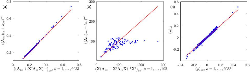
Figure 1: (a) Quality of approximation (25a ). (b) Quality of approximation (25b ). (c) Comparison of posterior means obtained by the diagonal-EP and the scalar-EP. Straight lines denote identity.
We assume that the expression level values { X n β k } subscript π π π \{X_{nk}\} are irregular enough
(arising from both biological and experimental variability) to be considered βrandomβ and that N π N and K πΎ K
are large enough to justify the application of the free probability approach. Then, TheoremΒ 1 offers the approximations for the fixed-point equations of diagonal-EP in (15 ) as
( ( π² 1 β w + πΏ β β π² 1 β z β πΏ ) β 1 ) k β k subscript superscript subscript π² 1 π€ superscript πΏ β subscript π² 1 π§ πΏ 1 π π \displaystyle(({\mathchoice{\mbox{\boldmath$\displaystyle\Lambda$}}{\mbox{\boldmath$\textstyle\Lambda$}}{\mbox{\boldmath$\scriptstyle\Lambda$}}{\mbox{\boldmath$\scriptscriptstyle\Lambda$}}}_{1w}+{\mathchoice{\mbox{\boldmath$\displaystyle X$}}{\mbox{\boldmath$\textstyle X$}}{\mbox{\boldmath$\scriptstyle X$}}{\mbox{\boldmath$\scriptscriptstyle X$}}}^{\dagger}{{\mathchoice{\mbox{\boldmath$\displaystyle\Lambda$}}{\mbox{\boldmath$\textstyle\Lambda$}}{\mbox{\boldmath$\scriptstyle\Lambda$}}{\mbox{\boldmath$\scriptscriptstyle\Lambda$}}}}_{1z}{\mathchoice{\mbox{\boldmath$\displaystyle X$}}{\mbox{\boldmath$\textstyle X$}}{\mbox{\boldmath$\scriptstyle X$}}{\mbox{\boldmath$\scriptscriptstyle X$}}})^{-1})_{kk}
β ( ( π² 1 β w ) k β k + Ξ» 2 β w ) β 1 absent superscript subscript subscript π² 1 π€ π π subscript π 2 π€ 1 \displaystyle\approx(({\mathchoice{\mbox{\boldmath$\displaystyle\Lambda$}}{\mbox{\boldmath$\textstyle\Lambda$}}{\mbox{\boldmath$\scriptstyle\Lambda$}}{\mbox{\boldmath$\scriptscriptstyle\Lambda$}}}_{1w})_{kk}+\lambda_{2w})^{-1}
(25a)
( πΏ β ( π² 1 β w + πΏ β β π² 1 β z β πΏ ) β 1 β πΏ β ) n β n subscript πΏ superscript subscript π² 1 π€ superscript πΏ β subscript π² 1 π§ πΏ 1 superscript πΏ β π π \displaystyle({\mathchoice{\mbox{\boldmath$\displaystyle X$}}{\mbox{\boldmath$\textstyle X$}}{\mbox{\boldmath$\scriptstyle X$}}{\mbox{\boldmath$\scriptscriptstyle X$}}}({\mathchoice{\mbox{\boldmath$\displaystyle\Lambda$}}{\mbox{\boldmath$\textstyle\Lambda$}}{\mbox{\boldmath$\scriptstyle\Lambda$}}{\mbox{\boldmath$\scriptscriptstyle\Lambda$}}}_{1w}+{\mathchoice{\mbox{\boldmath$\displaystyle X$}}{\mbox{\boldmath$\textstyle X$}}{\mbox{\boldmath$\scriptstyle X$}}{\mbox{\boldmath$\scriptscriptstyle X$}}}^{\dagger}{{\mathchoice{\mbox{\boldmath$\displaystyle\Lambda$}}{\mbox{\boldmath$\textstyle\Lambda$}}{\mbox{\boldmath$\scriptstyle\Lambda$}}{\mbox{\boldmath$\scriptscriptstyle\Lambda$}}}}_{1z}{\mathchoice{\mbox{\boldmath$\displaystyle X$}}{\mbox{\boldmath$\textstyle X$}}{\mbox{\boldmath$\scriptstyle X$}}{\mbox{\boldmath$\scriptscriptstyle X$}}})^{-1}{\mathchoice{\mbox{\boldmath$\displaystyle X$}}{\mbox{\boldmath$\textstyle X$}}{\mbox{\boldmath$\scriptstyle X$}}{\mbox{\boldmath$\scriptscriptstyle X$}}}^{\dagger})_{nn}
β ( ( π² 1 β z ) n β n + Ξ» 2 β z ) β 1 absent superscript subscript subscript π² 1 π§ π π subscript π 2 π§ 1 \displaystyle\approx(({\mathchoice{\mbox{\boldmath$\displaystyle\Lambda$}}{\mbox{\boldmath$\textstyle\Lambda$}}{\mbox{\boldmath$\scriptstyle\Lambda$}}{\mbox{\boldmath$\scriptscriptstyle\Lambda$}}}_{1z})_{nn}+\lambda_{2z})^{-1}
(25b)
where Ξ» 2 β w subscript π 2 π€ \lambda_{2w} and Ξ» 2 β z subscript π 2 π§ \lambda_{2z} are appropriately computed scalars which are asymptotically consistent with (23 ). In FigureΒ 1 -a) and -b) we illustrate the validity of the approximations in (25 ) on the prostate cancer microarray dataset [34 ] with N = 102 π 102 N=102 patients and K = 6033 πΎ 6033 K=6033 genes.
Approximation (25 ) is excellent for the large matrix, but
(as might be expected) yields cruder results for the comparably small matrix related to the small number of patients available. Nevertheless, such a mismatch may not necessarily have a deteriorating role to the approximate posterior of π π \textstyle w . To show this, we compare the posterior mean using the diagonal-EP denoted by π π \textstyle\mu and compare with the scalar-EP denoted by π ~ ~ π \tilde{{\mathchoice{\mbox{\boldmath$\displaystyle\mu$}}{\mbox{\boldmath$\textstyle\mu$}}{\mbox{\boldmath$\scriptstyle\mu$}}{\mbox{\boldmath$\scriptscriptstyle\mu$}}}} . As shown in FigureΒ 1-c both methods yield in fact close results.
Appendix B Proof of TheoremΒ 1
TheoremΒ 1 -1) follows directly from TheoremΒ 2 such that we have
Ξ» 2 β w = R πΏ β β π² 1 β z β πΏ β ( β Ο w ) . subscript π 2 π€ subscript R superscript πΏ β subscript π² 1 π§ πΏ subscript π π€ \lambda_{2w}={\rm R}_{{\mathchoice{\mbox{\boldmath$\displaystyle X$}}{\mbox{\boldmath$\textstyle X$}}{\mbox{\boldmath$\scriptstyle X$}}{\mbox{\boldmath$\scriptscriptstyle X$}}}^{\dagger}{\mathchoice{\mbox{\boldmath$\displaystyle\Lambda$}}{\mbox{\boldmath$\textstyle\Lambda$}}{\mbox{\boldmath$\scriptstyle\Lambda$}}{\mbox{\boldmath$\scriptscriptstyle\Lambda$}}}_{1z}{\mathchoice{\mbox{\boldmath$\displaystyle X$}}{\mbox{\boldmath$\textstyle X$}}{\mbox{\boldmath$\scriptstyle X$}}{\mbox{\boldmath$\scriptscriptstyle X$}}}}(-\chi_{w}).
(64)
As regards TheoremΒ 1 -2), we first underline the following points:
β’
By invoking the Woodbury Β matrixΒ inversionΒ lemma, for πΊ ~ β ( π² 1 β z β 1 + πΏ π² 1 β w β 1 β πΏ β ) β 1 β ~ πΊ superscript superscript subscript π² 1 π§ 1 superscript subscript πΏ π² 1 π€ 1 superscript πΏ β 1 \tilde{{\mathchoice{\mbox{\boldmath$\displaystyle\Sigma$}}{\mbox{\boldmath$\textstyle\Sigma$}}{\mbox{\boldmath$\scriptstyle\Sigma$}}{\mbox{\boldmath$\scriptscriptstyle\Sigma$}}}}\triangleq({\mathchoice{\mbox{\boldmath$\displaystyle\Lambda$}}{\mbox{\boldmath$\textstyle\Lambda$}}{\mbox{\boldmath$\scriptstyle\Lambda$}}{\mbox{\boldmath$\scriptscriptstyle\Lambda$}}}_{1z}^{-1}+{\mathchoice{\mbox{\boldmath$\displaystyle X$}}{\mbox{\boldmath$\textstyle X$}}{\mbox{\boldmath$\scriptstyle X$}}{\mbox{\boldmath$\scriptscriptstyle X$}}}{\mathchoice{\mbox{\boldmath$\displaystyle\Lambda$}}{\mbox{\boldmath$\textstyle\Lambda$}}{\mbox{\boldmath$\scriptstyle\Lambda$}}{\mbox{\boldmath$\scriptscriptstyle\Lambda$}}}_{1w}^{-1}{\mathchoice{\mbox{\boldmath$\displaystyle X$}}{\mbox{\boldmath$\textstyle X$}}{\mbox{\boldmath$\scriptstyle X$}}{\mbox{\boldmath$\scriptscriptstyle X$}}}^{\dagger})^{-1} we write
( πΊ ~ ) n β n subscript ~ πΊ π π \displaystyle(\tilde{{\mathchoice{\mbox{\boldmath$\displaystyle\Sigma$}}{\mbox{\boldmath$\textstyle\Sigma$}}{\mbox{\boldmath$\scriptstyle\Sigma$}}{\mbox{\boldmath$\scriptscriptstyle\Sigma$}}}})_{nn}
= ( π² 1 β z ) n β n β ( π² 1 β z 2 ) n β n β ( πΏ πΊ πΏ β ) n β n absent subscript subscript π² 1 π§ π π subscript superscript subscript π² 1 π§ 2 π π subscript superscript πΏ πΊ πΏ β π π \displaystyle=({\mathchoice{\mbox{\boldmath$\displaystyle\Lambda$}}{\mbox{\boldmath$\textstyle\Lambda$}}{\mbox{\boldmath$\scriptstyle\Lambda$}}{\mbox{\boldmath$\scriptscriptstyle\Lambda$}}}_{1z})_{nn}-({\mathchoice{\mbox{\boldmath$\displaystyle\Lambda$}}{\mbox{\boldmath$\textstyle\Lambda$}}{\mbox{\boldmath$\scriptstyle\Lambda$}}{\mbox{\boldmath$\scriptscriptstyle\Lambda$}}}_{1z}^{2})_{nn}({\mathchoice{\mbox{\boldmath$\displaystyle X$}}{\mbox{\boldmath$\textstyle X$}}{\mbox{\boldmath$\scriptstyle X$}}{\mbox{\boldmath$\scriptscriptstyle X$}}}{\mathchoice{\mbox{\boldmath$\displaystyle\Sigma$}}{\mbox{\boldmath$\textstyle\Sigma$}}{\mbox{\boldmath$\scriptstyle\Sigma$}}{\mbox{\boldmath$\scriptscriptstyle\Sigma$}}}{\mathchoice{\mbox{\boldmath$\displaystyle X$}}{\mbox{\boldmath$\textstyle X$}}{\mbox{\boldmath$\scriptstyle X$}}{\mbox{\boldmath$\scriptscriptstyle X$}}}^{\dagger})_{nn}
(65)
= ( π² 1 β z ) n β n β ( π² 1 β z 2 ) n β n ( π² 1 β z ) n β n + ( π² 2 β z ) n β n absent subscript subscript π² 1 π§ π π subscript superscript subscript π² 1 π§ 2 π π subscript subscript π² 1 π§ π π subscript subscript π² 2 π§ π π \displaystyle=({\mathchoice{\mbox{\boldmath$\displaystyle\Lambda$}}{\mbox{\boldmath$\textstyle\Lambda$}}{\mbox{\boldmath$\scriptstyle\Lambda$}}{\mbox{\boldmath$\scriptscriptstyle\Lambda$}}}_{1z})_{nn}-\frac{({\mathchoice{\mbox{\boldmath$\displaystyle\Lambda$}}{\mbox{\boldmath$\textstyle\Lambda$}}{\mbox{\boldmath$\scriptstyle\Lambda$}}{\mbox{\boldmath$\scriptscriptstyle\Lambda$}}}_{1z}^{2})_{nn}}{({\mathchoice{\mbox{\boldmath$\displaystyle\Lambda$}}{\mbox{\boldmath$\textstyle\Lambda$}}{\mbox{\boldmath$\scriptstyle\Lambda$}}{\mbox{\boldmath$\scriptscriptstyle\Lambda$}}}_{1z})_{nn}+({\mathchoice{\mbox{\boldmath$\displaystyle\Lambda$}}{\mbox{\boldmath$\textstyle\Lambda$}}{\mbox{\boldmath$\scriptstyle\Lambda$}}{\mbox{\boldmath$\scriptscriptstyle\Lambda$}}}_{2z})_{nn}}
(66)
= 1 ( π² 1 β z β 1 ) n β n + ( π² 2 β z β 1 ) n β n . absent 1 subscript superscript subscript π² 1 π§ 1 π π subscript superscript subscript π² 2 π§ 1 π π \displaystyle=\frac{1}{({{\mathchoice{\mbox{\boldmath$\displaystyle\Lambda$}}{\mbox{\boldmath$\textstyle\Lambda$}}{\mbox{\boldmath$\scriptstyle\Lambda$}}{\mbox{\boldmath$\scriptscriptstyle\Lambda$}}}_{1z}^{-1}})_{nn}+({{\mathchoice{\mbox{\boldmath$\displaystyle\Lambda$}}{\mbox{\boldmath$\textstyle\Lambda$}}{\mbox{\boldmath$\scriptstyle\Lambda$}}{\mbox{\boldmath$\scriptscriptstyle\Lambda$}}}_{2z}^{-1}})_{nn}}.
(67)
β’
A matrix π¨ = π¨ β π¨ superscript π¨ β {\mathchoice{\mbox{\boldmath$\displaystyle A$}}{\mbox{\boldmath$\textstyle A$}}{\mbox{\boldmath$\scriptstyle A$}}{\mbox{\boldmath$\scriptscriptstyle A$}}}={\mathchoice{\mbox{\boldmath$\displaystyle A$}}{\mbox{\boldmath$\textstyle A$}}{\mbox{\boldmath$\scriptstyle A$}}{\mbox{\boldmath$\scriptscriptstyle A$}}}^{\dagger} has a LED if, and only if the limiting Stieltjes transform G π¨ β ( z ) subscript G π¨ π§ {\rm G}_{{\mathchoice{\mbox{\boldmath$\displaystyle A$}}{\mbox{\boldmath$\textstyle A$}}{\mbox{\boldmath$\scriptstyle A$}}{\mbox{\boldmath$\scriptscriptstyle A$}}}}(z) (for z β β \ β π§ \ β β z\in\mathbb{C}\backslash\mathbb{R} ) exists[39 ] . On the other hand, for π¨ π¨ \textstyle A being invertible we have [38 ]
G π¨ β 1 β ( z ) = β z β 1 β ( 1 + z β 1 β G π¨ β ( z β 1 ) ) . subscript G superscript π¨ 1 π§ superscript π§ 1 1 superscript π§ 1 subscript G π¨ superscript π§ 1 {\rm G}_{{\mathchoice{\mbox{\boldmath$\displaystyle A$}}{\mbox{\boldmath$\textstyle A$}}{\mbox{\boldmath$\scriptstyle A$}}{\mbox{\boldmath$\scriptscriptstyle A$}}}^{-1}}(z)=-z^{-1}(1+z^{-1}{\rm G}_{{\mathchoice{\mbox{\boldmath$\displaystyle A$}}{\mbox{\boldmath$\textstyle A$}}{\mbox{\boldmath$\scriptstyle A$}}{\mbox{\boldmath$\scriptscriptstyle A$}}}}(z^{-1})).
(68)
Thus, π² 1 β w β 1 superscript subscript π² 1 π€ 1 {\mathchoice{\mbox{\boldmath$\displaystyle\Lambda$}}{\mbox{\boldmath$\textstyle\Lambda$}}{\mbox{\boldmath$\scriptstyle\Lambda$}}{\mbox{\boldmath$\scriptscriptstyle\Lambda$}}}_{1w}^{-1} and π² 1 β z β 1 superscript subscript π² 1 π§ 1 {\mathchoice{\mbox{\boldmath$\displaystyle\Lambda$}}{\mbox{\boldmath$\textstyle\Lambda$}}{\mbox{\boldmath$\scriptstyle\Lambda$}}{\mbox{\boldmath$\scriptscriptstyle\Lambda$}}}_{1z}^{-1} have LEDs as π² 1 β w subscript π² 1 π€ {\mathchoice{\mbox{\boldmath$\displaystyle\Lambda$}}{\mbox{\boldmath$\textstyle\Lambda$}}{\mbox{\boldmath$\scriptstyle\Lambda$}}{\mbox{\boldmath$\scriptscriptstyle\Lambda$}}}_{1w} Β andΒ π² 1 β z subscript π² 1 π§ {\mathchoice{\mbox{\boldmath$\displaystyle\Lambda$}}{\mbox{\boldmath$\textstyle\Lambda$}}{\mbox{\boldmath$\scriptstyle\Lambda$}}{\mbox{\boldmath$\scriptscriptstyle\Lambda$}}}_{1z} do.
β’
We write π² 1 β z β 1 superscript subscript π² 1 π§ 1 {\mathchoice{\mbox{\boldmath$\displaystyle\Lambda$}}{\mbox{\boldmath$\textstyle\Lambda$}}{\mbox{\boldmath$\scriptstyle\Lambda$}}{\mbox{\boldmath$\scriptscriptstyle\Lambda$}}}_{1z}^{-1} of the form β n = 0 N β 1 Ξ± n β π² 1 β z n superscript subscript π 0 π 1 subscript πΌ π superscript subscript π² 1 π§ π \sum_{n=0}^{N-1}\alpha_{n}{\mathchoice{\mbox{\boldmath$\displaystyle\Lambda$}}{\mbox{\boldmath$\textstyle\Lambda$}}{\mbox{\boldmath$\scriptstyle\Lambda$}}{\mbox{\boldmath$\scriptscriptstyle\Lambda$}}}_{1z}^{n} for some Ξ± n subscript πΌ π \alpha_{n} (depending on the spectral moments Tr β ( π² 1 β z k ) Tr superscript subscript π² 1 π§ π {\rm Tr}({\mathchoice{\mbox{\boldmath$\displaystyle\Lambda$}}{\mbox{\boldmath$\textstyle\Lambda$}}{\mbox{\boldmath$\scriptstyle\Lambda$}}{\mbox{\boldmath$\scriptscriptstyle\Lambda$}}}_{1z}^{k}) up to some order). Thereby, it follows from DefinitionΒ 1 that πΏ π² 1 β w β 1 β πΏ β superscript subscript πΏ π² 1 π€ 1 superscript πΏ β {\mathchoice{\mbox{\boldmath$\displaystyle X$}}{\mbox{\boldmath$\textstyle X$}}{\mbox{\boldmath$\scriptstyle X$}}{\mbox{\boldmath$\scriptscriptstyle X$}}}{\mathchoice{\mbox{\boldmath$\displaystyle\Lambda$}}{\mbox{\boldmath$\textstyle\Lambda$}}{\mbox{\boldmath$\scriptstyle\Lambda$}}{\mbox{\boldmath$\scriptscriptstyle\Lambda$}}}_{1w}^{-1}{\mathchoice{\mbox{\boldmath$\displaystyle X$}}{\mbox{\boldmath$\textstyle X$}}{\mbox{\boldmath$\scriptstyle X$}}{\mbox{\boldmath$\scriptscriptstyle X$}}}^{\dagger} and π² 1 β z β 1 superscript subscript π² 1 π§ 1 {\mathchoice{\mbox{\boldmath$\displaystyle\Lambda$}}{\mbox{\boldmath$\textstyle\Lambda$}}{\mbox{\boldmath$\scriptstyle\Lambda$}}{\mbox{\boldmath$\scriptscriptstyle\Lambda$}}}_{1z}^{-1} are asymptotically free as the former matrix is assumed to be free of the inverse of the latter.
From these remarks TheoremΒ 1 -2) follows from TheoremΒ 2 such that we have
Ξ» 2 β z = 1 R πΏ π² 1 β w β 1 β πΏ β β ( β Ο ~ z ) β Β withΒ β Ο ~ z β Ο β ( πΊ ~ ) . subscript π 2 π§ 1 subscript R superscript subscript πΏ π² 1 π€ 1 superscript πΏ β subscript ~ π π§ Β withΒ subscript ~ π π§ β italic-Ο ~ πΊ \displaystyle\lambda_{2z}=\frac{1}{{\rm R}_{{\mathchoice{\mbox{\boldmath$\displaystyle X$}}{\mbox{\boldmath$\textstyle X$}}{\mbox{\boldmath$\scriptstyle X$}}{\mbox{\boldmath$\scriptscriptstyle X$}}}{\mathchoice{\mbox{\boldmath$\displaystyle\Lambda$}}{\mbox{\boldmath$\textstyle\Lambda$}}{\mbox{\boldmath$\scriptstyle\Lambda$}}{\mbox{\boldmath$\scriptscriptstyle\Lambda$}}}_{1w}^{-1}{\mathchoice{\mbox{\boldmath$\displaystyle X$}}{\mbox{\boldmath$\textstyle X$}}{\mbox{\boldmath$\scriptstyle X$}}{\mbox{\boldmath$\scriptscriptstyle X$}}}^{\dagger}}(-\tilde{\chi}_{z})}~{}\text{ with }\tilde{\chi}_{z}\triangleq\phi(\tilde{{\mathchoice{\mbox{\boldmath$\displaystyle\Sigma$}}{\mbox{\boldmath$\textstyle\Sigma$}}{\mbox{\boldmath$\scriptstyle\Sigma$}}{\mbox{\boldmath$\scriptscriptstyle\Sigma$}}}}).
(69)
Here, we note that since ( π² 1 β z + Ξ» 2 β z β π ) β 1 superscript subscript π² 1 π§ subscript π 2 π§ π 1 ({\mathchoice{\mbox{\boldmath$\displaystyle\Lambda$}}{\mbox{\boldmath$\textstyle\Lambda$}}{\mbox{\boldmath$\scriptstyle\Lambda$}}{\mbox{\boldmath$\scriptscriptstyle\Lambda$}}}_{1z}+\lambda_{2z}{\bf I})^{-1} has an (a.s.) asymptotically bounded spectral norm so does
( π² 1 β z β 1 + Ξ» 2 β z β 1 β π ) β 1 = Ξ» 2 β z β π β Ξ» 2 β z 2 β ( π² 1 β z + Ξ» 2 β z β π ) β 1 . superscript superscript subscript π² 1 π§ 1 superscript subscript π 2 π§ 1 π 1 subscript π 2 π§ π superscript subscript π 2 π§ 2 superscript subscript π² 1 π§ subscript π 2 π§ π 1 ({\mathchoice{\mbox{\boldmath$\displaystyle\Lambda$}}{\mbox{\boldmath$\textstyle\Lambda$}}{\mbox{\boldmath$\scriptstyle\Lambda$}}{\mbox{\boldmath$\scriptscriptstyle\Lambda$}}}_{1z}^{-1}+\lambda_{2z}^{-1}{\bf I})^{-1}=\lambda_{2z}{\bf I}-\lambda_{2z}^{2}({\mathchoice{\mbox{\boldmath$\displaystyle\Lambda$}}{\mbox{\boldmath$\textstyle\Lambda$}}{\mbox{\boldmath$\scriptstyle\Lambda$}}{\mbox{\boldmath$\scriptscriptstyle\Lambda$}}}_{1z}+\lambda_{2z}{\bf I})^{-1}.
(70)
Moreover, from (70 ) it follows that
Ο ~ z = Ξ» 2 β z β ( 1 β Ξ» 2 β z β Ο z ) . subscript ~ π z subscript π 2 π§ 1 subscript π 2 π§ subscript π π§ \tilde{\chi}_{\rm z}=\lambda_{2z}(1-\lambda_{2z}\chi_{z}).
(71)
To complete the proof we only need to show that Ξ» 2 β w subscript π 2 π€ \lambda_{2w} in (64 ) and Ξ» 2 β z subscript π 2 π§ \lambda_{2z} in (69 ) fulfill the system of equations in (23 ). To this end we outline two remarks whose proofs are given at the end of the appendix, for convenience.
We thereby complete the proof by showing that the two solutions (i) Ξ» ~ 1 β w = Ξ» 1 β w subscript ~ π 1 π€ subscript π 1 π€ \tilde{\lambda}_{1w}=\lambda_{1w} and (ii) Ξ» ~ 1 β z = Ξ» 1 β z subscript ~ π 1 π§ subscript π 1 π§ \tilde{\lambda}_{1z}=\lambda_{1z} are consistent . To this end, we postulate that
Ξ» 2 β w β Ο w = Ξ± β ( 1 β Ξ» 2 β z β Ο z ) . subscript π 2 π€ subscript π π€ πΌ 1 subscript π 2 π§ subscript π π§ \lambda_{2w}\chi_{w}{=}\alpha(1-\lambda_{2z}\chi_{z}).
(76)
We first obtain (i) and (ii) under the hypothesis (76 ); then we show the hypothesis holds when (i) and (ii) hold.
By using respectively the first equality of (73 ), (76 ) and the first equalities in (74 ) and (75 ) we obtain that
1 Ξ» 1 β z 1 subscript π 1 π§ \displaystyle\frac{1}{\lambda_{1z}}
= S π² 1 β z β ( β ( 1 β Ξ» 2 β z β Ο z ) ) absent subscript S subscript π² 1 π§ 1 subscript π 2 π§ subscript π π§ \displaystyle={\rm S}_{{\mathchoice{\mbox{\boldmath$\displaystyle\Lambda$}}{\mbox{\boldmath$\textstyle\Lambda$}}{\mbox{\boldmath$\scriptstyle\Lambda$}}{\mbox{\boldmath$\scriptscriptstyle\Lambda$}}}_{1z}}(-(1-\lambda_{2z}\chi_{z}))
(77)
= S π² 1 β z β ( β Ξ» ~ 1 β z β Ο z ) absent subscript S subscript π² 1 π§ subscript ~ π 1 π§ subscript π π§ \displaystyle={\rm S}_{{\mathchoice{\mbox{\boldmath$\displaystyle\Lambda$}}{\mbox{\boldmath$\textstyle\Lambda$}}{\mbox{\boldmath$\scriptstyle\Lambda$}}{\mbox{\boldmath$\scriptscriptstyle\Lambda$}}}_{1z}}(-\tilde{\lambda}_{1z}\chi_{z})
(78)
= S π² 1 β z β ( β R π² 1 β z β ( β Ο z ) β Ο z ) . absent subscript S subscript π² 1 π§ subscript R subscript π² 1 π§ subscript π π§ subscript π π§ \displaystyle={\rm S}_{{\mathchoice{\mbox{\boldmath$\displaystyle\Lambda$}}{\mbox{\boldmath$\textstyle\Lambda$}}{\mbox{\boldmath$\scriptstyle\Lambda$}}{\mbox{\boldmath$\scriptscriptstyle\Lambda$}}}_{1z}}(-{\rm R}_{{\mathchoice{\mbox{\boldmath$\displaystyle\Lambda$}}{\mbox{\boldmath$\textstyle\Lambda$}}{\mbox{\boldmath$\scriptstyle\Lambda$}}{\mbox{\boldmath$\scriptscriptstyle\Lambda$}}}_{1z}}(-\chi_{z})\chi_{z}).
(79)
From (28 ), this implies that Ξ» 1 β z = R π² 1 β z β ( β Ο z ) subscript π 1 π§ subscript R subscript π² 1 π§ subscript π π§ \lambda_{1z}={\rm R}_{{\mathchoice{\mbox{\boldmath$\displaystyle\Lambda$}}{\mbox{\boldmath$\textstyle\Lambda$}}{\mbox{\boldmath$\scriptstyle\Lambda$}}{\mbox{\boldmath$\scriptscriptstyle\Lambda$}}}_{1z}}(-\chi_{z}) , i.e. Ξ» 1 β z = Ξ» ~ 1 β z subscript π 1 π§ subscript ~ π 1 π§ \lambda_{1z}=\tilde{\lambda}_{1z} .
By using respectively the second equality of (73 ), (71 ), (76 ) and (28 ) we obtain that
Ξ» ~ 1 β w subscript ~ π 1 π€ \displaystyle\tilde{\lambda}_{1w}
= S π² 1 β w β 1 β ( β Ξ± β ( 1 β Ξ» 2 β z β Ο z ) ) absent subscript S superscript subscript π² 1 π€ 1 πΌ 1 subscript π 2 π§ subscript π π§ \displaystyle={\rm S}_{{\mathchoice{\mbox{\boldmath$\displaystyle\Lambda$}}{\mbox{\boldmath$\textstyle\Lambda$}}{\mbox{\boldmath$\scriptstyle\Lambda$}}{\mbox{\boldmath$\scriptscriptstyle\Lambda$}}}_{1w}^{-1}}\left(-\alpha(1-\lambda_{2z}\chi_{z})\right)
(80)
= S π² 1 β w β 1 β ( β Ξ» 2 β w β Ο w ) absent subscript S superscript subscript π² 1 π€ 1 subscript π 2 π€ subscript π π€ \displaystyle={\rm S}_{{\mathchoice{\mbox{\boldmath$\displaystyle\Lambda$}}{\mbox{\boldmath$\textstyle\Lambda$}}{\mbox{\boldmath$\scriptstyle\Lambda$}}{\mbox{\boldmath$\scriptscriptstyle\Lambda$}}}_{1w}^{-1}}\left(-\lambda_{2w}\chi_{w}\right)
(81)
= S π² 1 β w β 1 β ( β ( 1 β Ξ» 1 β w β Ο w ) ) absent subscript S superscript subscript π² 1 π€ 1 1 subscript π 1 π€ subscript π π€ \displaystyle={\rm S}_{{\mathchoice{\mbox{\boldmath$\displaystyle\Lambda$}}{\mbox{\boldmath$\textstyle\Lambda$}}{\mbox{\boldmath$\scriptstyle\Lambda$}}{\mbox{\boldmath$\scriptscriptstyle\Lambda$}}}_{1w}^{-1}}\left(-(1-\lambda_{1w}\chi_{w})\right)
(82)
= 1 R π² 1 β w β 1 β ( Ξ» ~ 1 β w β ( 1 β Ξ» 1 β w β Ο w ) ) . absent 1 subscript R superscript subscript π² 1 π€ 1 subscript ~ π 1 π€ 1 subscript π 1 π€ subscript π π€ \displaystyle=\frac{1}{{\rm R}_{{\mathchoice{\mbox{\boldmath$\displaystyle\Lambda$}}{\mbox{\boldmath$\textstyle\Lambda$}}{\mbox{\boldmath$\scriptstyle\Lambda$}}{\mbox{\boldmath$\scriptscriptstyle\Lambda$}}}_{1w}^{-1}}(\tilde{\lambda}_{1w}(1-\lambda_{1w}\chi_{w}))}.
(83)
From LemmaΒ 2 the equality Ξ» ~ 1 β w = R π² 1 β w β ( β Ο w ) subscript ~ π 1 π€ subscript R subscript π² 1 π€ subscript π π€ \tilde{\lambda}_{1w}={\rm R}_{{\mathchoice{\mbox{\boldmath$\displaystyle\Lambda$}}{\mbox{\boldmath$\textstyle\Lambda$}}{\mbox{\boldmath$\scriptstyle\Lambda$}}{\mbox{\boldmath$\scriptscriptstyle\Lambda$}}}_{1w}}(-\chi_{w}) , i.e. Ξ» ~ 1 β w = Ξ» 1 β w subscript ~ π 1 π€ subscript π 1 π€ \tilde{\lambda}_{1w}=\lambda_{1w} , fulfills (83 ) and thereby the solution (ii) is consistent too.
We complete the proof by showing that the hypothesis (76 ) holds when (i) and (ii) hold:
Ξ» 2 β w β Ο w subscript π 2 π€ subscript π π€ \displaystyle\lambda_{2w}\chi_{w}
= 1 β Ξ» 1 β w β Ο w absent 1 subscript π 1 π€ subscript π π€ \displaystyle=1-\lambda_{1w}\chi_{w}
(84)
= Ο β ( π β Ξ» 1 β w β ( Ξ» 1 β w β π + Ξ» 1 β z β πΏ β β πΏ ) β 1 ) absent italic-Ο π subscript π 1 π€ superscript subscript π 1 π€ π subscript π 1 π§ superscript πΏ β πΏ 1 \displaystyle=\phi({\bf I}-\lambda_{1w}(\lambda_{1w}{\bf I}+\lambda_{1z}{\mathchoice{\mbox{\boldmath$\displaystyle X$}}{\mbox{\boldmath$\textstyle X$}}{\mbox{\boldmath$\scriptstyle X$}}{\mbox{\boldmath$\scriptscriptstyle X$}}}^{\dagger}{\mathchoice{\mbox{\boldmath$\displaystyle X$}}{\mbox{\boldmath$\textstyle X$}}{\mbox{\boldmath$\scriptstyle X$}}{\mbox{\boldmath$\scriptscriptstyle X$}}})^{-1})
(85)
= Ξ± β Ο β ( π β Ξ» 1 β w β ( Ξ» 1 β w β π + Ξ» 1 β z β πΏ πΏ β ) β 1 ) absent πΌ italic-Ο π subscript π 1 π€ superscript subscript π 1 π€ π subscript π 1 π§ superscript πΏ πΏ β 1 \displaystyle=\alpha\phi({\bf I}-\lambda_{1w}(\lambda_{1w}{\bf I}+\lambda_{1z}{\mathchoice{\mbox{\boldmath$\displaystyle X$}}{\mbox{\boldmath$\textstyle X$}}{\mbox{\boldmath$\scriptstyle X$}}{\mbox{\boldmath$\scriptscriptstyle X$}}}{\mathchoice{\mbox{\boldmath$\displaystyle X$}}{\mbox{\boldmath$\textstyle X$}}{\mbox{\boldmath$\scriptstyle X$}}{\mbox{\boldmath$\scriptscriptstyle X$}}}^{\dagger})^{-1})
(86)
= Ξ± β Ο β ( π β Ξ» 1 β z β 1 β ( Ξ» 1 β z β 1 β π + Ξ» 1 β w β 1 β πΏ πΏ β ) β 1 ) absent πΌ italic-Ο π superscript subscript π 1 π§ 1 superscript superscript subscript π 1 π§ 1 π superscript subscript π 1 π€ 1 superscript πΏ πΏ β 1 \displaystyle=\alpha\phi({\bf I}-\lambda_{1z}^{-1}(\lambda_{1z}^{\small-1}{\bf I}+{\lambda_{1w}^{\small-1}}{\mathchoice{\mbox{\boldmath$\displaystyle X$}}{\mbox{\boldmath$\textstyle X$}}{\mbox{\boldmath$\scriptstyle X$}}{\mbox{\boldmath$\scriptscriptstyle X$}}}{\mathchoice{\mbox{\boldmath$\displaystyle X$}}{\mbox{\boldmath$\textstyle X$}}{\mbox{\boldmath$\scriptstyle X$}}{\mbox{\boldmath$\scriptscriptstyle X$}}}^{\dagger})^{-1})
(87)
= Ξ± β Ο β ( π β ( π β Ξ» 1 β z β πΏ β ( Ξ» 1 β w + Ξ» 1 β z β πΏ β β πΏ ) β 1 β πΏ β ) ) absent πΌ italic-Ο π π subscript π 1 π§ πΏ superscript subscript π 1 π€ subscript π 1 π§ superscript πΏ β πΏ 1 superscript πΏ β \displaystyle=\alpha\phi({\bf I}-({\bf I}-\lambda_{1z}{\mathchoice{\mbox{\boldmath$\displaystyle X$}}{\mbox{\boldmath$\textstyle X$}}{\mbox{\boldmath$\scriptstyle X$}}{\mbox{\boldmath$\scriptscriptstyle X$}}}(\lambda_{1w}+\lambda_{1z}{\mathchoice{\mbox{\boldmath$\displaystyle X$}}{\mbox{\boldmath$\textstyle X$}}{\mbox{\boldmath$\scriptstyle X$}}{\mbox{\boldmath$\scriptscriptstyle X$}}}^{\dagger}{\mathchoice{\mbox{\boldmath$\displaystyle X$}}{\mbox{\boldmath$\textstyle X$}}{\mbox{\boldmath$\scriptstyle X$}}{\mbox{\boldmath$\scriptscriptstyle X$}}})^{-1}{\mathchoice{\mbox{\boldmath$\displaystyle X$}}{\mbox{\boldmath$\textstyle X$}}{\mbox{\boldmath$\scriptstyle X$}}{\mbox{\boldmath$\scriptscriptstyle X$}}}^{\dagger}))
(88)
= Ξ± β ( 1 β ( 1 β Ξ» 1 β z β Ο z ) ) absent πΌ 1 1 subscript π 1 π§ subscript π π§ \displaystyle=\alpha(1-(1-\lambda_{1z}\chi_{z}))
(89)
= Ξ± β ( 1 β Ξ» 2 β z β Ο z ) . absent πΌ 1 subscript π 2 π§ subscript π π§ \displaystyle=\alpha(1-\lambda_{2z}\chi_{z}).
(90)
Here (88 ) follows from the WoodburyΒ matrixΒ inversionΒ lemma.
B-A Proof of RemarkΒ 1
From LemmaΒ 1 we have
Ο w = ( Ξ» 1 β w + Ξ» 2 β w ) β 1 . subscript π π€ superscript subscript π 1 π€ subscript π 2 π€ 1 \chi_{w}=(\lambda_{1w}+\lambda_{2w})^{-1}.
(91)
With the scaling property of the R-transform (see [26 , TableΒ 4] ), the equality Ξ» 2 β w = R πΏ β β π² 1 β z β πΏ β ( β Ο w ) subscript π 2 π€ subscript R superscript πΏ β subscript π² 1 π§ πΏ subscript π π€ {\lambda}_{2w}={\rm R}_{{\mathchoice{\mbox{\boldmath$\displaystyle X$}}{\mbox{\boldmath$\textstyle X$}}{\mbox{\boldmath$\scriptstyle X$}}{\mbox{\boldmath$\scriptscriptstyle X$}}}^{\dagger}{\mathchoice{\mbox{\boldmath$\displaystyle\Lambda$}}{\mbox{\boldmath$\textstyle\Lambda$}}{\mbox{\boldmath$\scriptstyle\Lambda$}}{\mbox{\boldmath$\scriptscriptstyle\Lambda$}}}_{1z}{\mathchoice{\mbox{\boldmath$\displaystyle X$}}{\mbox{\boldmath$\textstyle X$}}{\mbox{\boldmath$\scriptstyle X$}}{\mbox{\boldmath$\scriptscriptstyle X$}}}}(-\chi_{w}) holds if, and only if
1 = R 1 Ξ» 2 β w β πΏ β β π² 1 β z β πΏ β ( β Ξ» 2 β w β Ο w ) . 1 subscript R 1 subscript π 2 π€ superscript πΏ β subscript π² 1 π§ πΏ subscript π 2 π€ subscript π π€ 1={\rm R}_{\frac{1}{{\lambda}_{2w}}{\mathchoice{\mbox{\boldmath$\displaystyle X$}}{\mbox{\boldmath$\textstyle X$}}{\mbox{\boldmath$\scriptstyle X$}}{\mbox{\boldmath$\scriptscriptstyle X$}}}^{\dagger}{\mathchoice{\mbox{\boldmath$\displaystyle\Lambda$}}{\mbox{\boldmath$\textstyle\Lambda$}}{\mbox{\boldmath$\scriptstyle\Lambda$}}{\mbox{\boldmath$\scriptscriptstyle\Lambda$}}}_{1z}{\mathchoice{\mbox{\boldmath$\displaystyle X$}}{\mbox{\boldmath$\textstyle X$}}{\mbox{\boldmath$\scriptstyle X$}}{\mbox{\boldmath$\scriptscriptstyle X$}}}}(-{\lambda}_{2w}\chi_{w}).
(92)
We express this result in terms of the S-transform via (28 ) as:
1 1 \displaystyle 1
= S 1 Ξ» 2 β w β πΏ β β π² 1 β z β πΏ β ( β Ξ» 2 β w β Ο w ) absent subscript S 1 subscript π 2 π€ superscript πΏ β subscript π² 1 π§ πΏ subscript π 2 π€ subscript π π€ \displaystyle={\rm S}_{\frac{1}{{\lambda}_{2w}}{\mathchoice{\mbox{\boldmath$\displaystyle X$}}{\mbox{\boldmath$\textstyle X$}}{\mbox{\boldmath$\scriptstyle X$}}{\mbox{\boldmath$\scriptscriptstyle X$}}}^{\dagger}{\mathchoice{\mbox{\boldmath$\displaystyle\Lambda$}}{\mbox{\boldmath$\textstyle\Lambda$}}{\mbox{\boldmath$\scriptstyle\Lambda$}}{\mbox{\boldmath$\scriptscriptstyle\Lambda$}}}_{1z}{\mathchoice{\mbox{\boldmath$\displaystyle X$}}{\mbox{\boldmath$\textstyle X$}}{\mbox{\boldmath$\scriptstyle X$}}{\mbox{\boldmath$\scriptscriptstyle X$}}}}(-{\lambda}_{2w}\chi_{w})
(93)
= S 1 Ξ» 2 β w β π² 1 β z β πΏ πΏ β β ( β Ξ» 2 β w β Ο w Ξ± ) absent subscript S 1 subscript π 2 π€ subscript π² 1 π§ superscript πΏ πΏ β subscript π 2 π€ subscript π π€ πΌ \displaystyle={\rm S}_{\frac{1}{{\lambda}_{2w}}{\mathchoice{\mbox{\boldmath$\displaystyle\Lambda$}}{\mbox{\boldmath$\textstyle\Lambda$}}{\mbox{\boldmath$\scriptstyle\Lambda$}}{\mbox{\boldmath$\scriptscriptstyle\Lambda$}}}_{1z}{\mathchoice{\mbox{\boldmath$\displaystyle X$}}{\mbox{\boldmath$\textstyle X$}}{\mbox{\boldmath$\scriptstyle X$}}{\mbox{\boldmath$\scriptscriptstyle X$}}}{\mathchoice{\mbox{\boldmath$\displaystyle X$}}{\mbox{\boldmath$\textstyle X$}}{\mbox{\boldmath$\scriptstyle X$}}{\mbox{\boldmath$\scriptscriptstyle X$}}}^{\dagger}}\left(-\frac{{\lambda}_{2w}\chi_{w}}{\alpha}\right)
(94)
= S π² 1 β z β ( β Ξ» 2 β w β Ο w Ξ± ) β Ξ» 1 β z β 1 β S 1 Ξ» 2 β w β πΏ πΏ β β ( β Ξ» 2 β w β Ο w Ξ± ) absent subscript β subscript S subscript π² 1 π§ subscript π 2 π€ subscript π π€ πΌ superscript subscript π 1 π§ 1 subscript S 1 subscript π 2 π€ superscript πΏ πΏ β subscript π 2 π€ subscript π π€ πΌ \displaystyle=\underbrace{{\rm S}_{{\mathchoice{\mbox{\boldmath$\displaystyle\Lambda$}}{\mbox{\boldmath$\textstyle\Lambda$}}{\mbox{\boldmath$\scriptstyle\Lambda$}}{\mbox{\boldmath$\scriptscriptstyle\Lambda$}}}_{1z}}\left(-\frac{{\lambda}_{2w}\chi_{w}}{\alpha}\right)}_{\lambda_{1z}^{-1}}{\rm S}_{\frac{1}{{\lambda}_{2w}}{\mathchoice{\mbox{\boldmath$\displaystyle X$}}{\mbox{\boldmath$\textstyle X$}}{\mbox{\boldmath$\scriptstyle X$}}{\mbox{\boldmath$\scriptscriptstyle X$}}}{\mathchoice{\mbox{\boldmath$\displaystyle X$}}{\mbox{\boldmath$\textstyle X$}}{\mbox{\boldmath$\scriptstyle X$}}{\mbox{\boldmath$\scriptscriptstyle X$}}}^{\dagger}}\left(-\frac{{\lambda}_{2w}\chi_{w}}{\alpha}\right)
(95)
= S Ξ» 1 β z Ξ» 2 β w β πΏ πΏ β β ( β Ξ» 2 β w β Ο w Ξ± ) absent subscript S subscript π 1 π§ subscript π 2 π€ superscript πΏ πΏ β subscript π 2 π€ subscript π π€ πΌ \displaystyle={\rm S}_{\frac{\lambda_{1z}}{{\lambda}_{2w}}{\mathchoice{\mbox{\boldmath$\displaystyle X$}}{\mbox{\boldmath$\textstyle X$}}{\mbox{\boldmath$\scriptstyle X$}}{\mbox{\boldmath$\scriptscriptstyle X$}}}{\mathchoice{\mbox{\boldmath$\displaystyle X$}}{\mbox{\boldmath$\textstyle X$}}{\mbox{\boldmath$\scriptstyle X$}}{\mbox{\boldmath$\scriptscriptstyle X$}}}^{\dagger}}\left(-\frac{{\lambda}_{2w}\chi_{w}}{\alpha}\right)
(96)
= S Ξ» 1 β z Ξ» 2 β w β πΏ β β πΏ β ( β Ξ» 2 β w β Ο w ) . absent subscript S subscript π 1 π§ subscript π 2 π€ superscript πΏ β πΏ subscript π 2 π€ subscript π π€ \displaystyle={\rm S}_{\frac{\lambda_{1z}}{{\lambda}_{2w}}{\mathchoice{\mbox{\boldmath$\displaystyle X$}}{\mbox{\boldmath$\textstyle X$}}{\mbox{\boldmath$\scriptstyle X$}}{\mbox{\boldmath$\scriptscriptstyle X$}}}^{\dagger}{\mathchoice{\mbox{\boldmath$\displaystyle X$}}{\mbox{\boldmath$\textstyle X$}}{\mbox{\boldmath$\scriptstyle X$}}{\mbox{\boldmath$\scriptscriptstyle X$}}}}(-{\lambda}_{2w}\chi_{w}).
(97)
Here (95 ) follows from (c) and the multiplicative free convolution (34 ). We now reuse (28 ) to express (97 ) in terms of the R-transform as
Ξ» 2 β w = R Ξ» 1 β z β πΏ β β πΏ β ( β Ο w ) . subscript π 2 π€ subscript R subscript π 1 π§ superscript πΏ β πΏ subscript π π€ {\lambda}_{2w}={\rm R}_{\lambda_{1z}{\mathchoice{\mbox{\boldmath$\displaystyle X$}}{\mbox{\boldmath$\textstyle X$}}{\mbox{\boldmath$\scriptstyle X$}}{\mbox{\boldmath$\scriptscriptstyle X$}}}^{\dagger}{\mathchoice{\mbox{\boldmath$\displaystyle X$}}{\mbox{\boldmath$\textstyle X$}}{\mbox{\boldmath$\scriptstyle X$}}{\mbox{\boldmath$\scriptscriptstyle X$}}}}(-\chi_{w}).
(98)
This completes the proof.
B-B Proof of RemarkΒ 2
We make use of RemarkΒ 1 for a different βsystemβ as
Ο β ( ( π² 1 β z β 1 + πΏ π² 1 β w β 1 β πΏ β ) β 1 ) = Ο β ( ( Ξ» ~ 1 β z β 1 β π + Ξ» ~ 1 β w β 1 β πΏ πΏ β ) β 1 ) italic-Ο superscript superscript subscript π² 1 π§ 1 superscript subscript πΏ π² 1 π€ 1 superscript πΏ β 1 italic-Ο superscript superscript subscript ~ π 1 π§ 1 π superscript subscript ~ π 1 π€ 1 superscript πΏ πΏ β 1 \displaystyle\phi(({\mathchoice{\mbox{\boldmath$\displaystyle\Lambda$}}{\mbox{\boldmath$\textstyle\Lambda$}}{\mbox{\boldmath$\scriptstyle\Lambda$}}{\mbox{\boldmath$\scriptscriptstyle\Lambda$}}}_{1z}^{-1}+{\mathchoice{\mbox{\boldmath$\displaystyle X$}}{\mbox{\boldmath$\textstyle X$}}{\mbox{\boldmath$\scriptstyle X$}}{\mbox{\boldmath$\scriptscriptstyle X$}}}{\mathchoice{\mbox{\boldmath$\displaystyle\Lambda$}}{\mbox{\boldmath$\textstyle\Lambda$}}{\mbox{\boldmath$\scriptstyle\Lambda$}}{\mbox{\boldmath$\scriptscriptstyle\Lambda$}}}_{1w}^{-1}{\mathchoice{\mbox{\boldmath$\displaystyle X$}}{\mbox{\boldmath$\textstyle X$}}{\mbox{\boldmath$\scriptstyle X$}}{\mbox{\boldmath$\scriptscriptstyle X$}}}^{\dagger})^{-1})=\phi((\tilde{\lambda}_{1z}^{-1}{\bf I}+{\tilde{\lambda}_{1w}^{-1}}{\mathchoice{\mbox{\boldmath$\displaystyle X$}}{\mbox{\boldmath$\textstyle X$}}{\mbox{\boldmath$\scriptstyle X$}}{\mbox{\boldmath$\scriptscriptstyle X$}}}{\mathchoice{\mbox{\boldmath$\displaystyle X$}}{\mbox{\boldmath$\textstyle X$}}{\mbox{\boldmath$\scriptstyle X$}}{\mbox{\boldmath$\scriptscriptstyle X$}}}^{\dagger})^{-1})
(99)
such that we have
Ο ~ z = 1 Ξ» ~ 1 β z β 1 + Ξ» 2 β z β 1 = Ο β ( ( Ξ» ~ 1 β z β 1 β π + Ξ» ~ 1 β w β 1 β πΏ πΏ β ) β 1 ) subscript ~ π π§ 1 superscript subscript ~ π 1 π§ 1 superscript subscript π 2 π§ 1 italic-Ο superscript superscript subscript ~ π 1 π§ 1 π superscript subscript ~ π 1 π€ 1 superscript πΏ πΏ β 1 \tilde{\chi}_{z}=\frac{1}{\tilde{\lambda}_{1z}^{-1}+\lambda_{2z}^{-1}}=\phi((\tilde{\lambda}_{1z}^{-1}{\bf I}+\tilde{\lambda}_{1w}^{-1}{\mathchoice{\mbox{\boldmath$\displaystyle X$}}{\mbox{\boldmath$\textstyle X$}}{\mbox{\boldmath$\scriptstyle X$}}{\mbox{\boldmath$\scriptscriptstyle X$}}}{\mathchoice{\mbox{\boldmath$\displaystyle X$}}{\mbox{\boldmath$\textstyle X$}}{\mbox{\boldmath$\scriptstyle X$}}{\mbox{\boldmath$\scriptscriptstyle X$}}}^{\dagger})^{-1})
(100)
where
Ξ» ~ 1 β z β 1 R π² 1 β z β 1 β ( β Ο ~ z ) β Β andΒ β Ξ» ~ 1 β w β S π² 1 β w β 1 β ( β Ξ± β Ο ~ z Ξ» 2 β z ) . β subscript ~ π 1 π§ 1 subscript R superscript subscript π² 1 π§ 1 subscript ~ π π§ Β andΒ subscript ~ π 1 π€ β subscript S superscript subscript π² 1 π€ 1 πΌ subscript ~ π π§ subscript π 2 π§ \tilde{\lambda}_{1z}\triangleq\frac{1}{{\rm R}_{{\mathchoice{\mbox{\boldmath$\displaystyle\Lambda$}}{\mbox{\boldmath$\textstyle\Lambda$}}{\mbox{\boldmath$\scriptstyle\Lambda$}}{\mbox{\boldmath$\scriptscriptstyle\Lambda$}}}_{1z}^{-1}}(-\tilde{\chi}_{z})}~{}\text{~{}and~{}}\tilde{\lambda}_{1w}\triangleq{\rm S}_{{\mathchoice{\mbox{\boldmath$\displaystyle\Lambda$}}{\mbox{\boldmath$\textstyle\Lambda$}}{\mbox{\boldmath$\scriptstyle\Lambda$}}{\mbox{\boldmath$\scriptscriptstyle\Lambda$}}}_{1w}^{-1}}\left(-\frac{\alpha\tilde{\chi}_{z}}{\lambda_{2z}}\right).
(101)
By invoking the first equality of (100 ) to the definition of Ο z subscript π π§ \chi_{z} we get Ο z = 1 / ( Ξ» ~ 1 β z + Ξ» 2 β z ) subscript π π§ 1 subscript ~ π 1 π§ subscript π 2 π§ \chi_{z}=1/(\tilde{\lambda}_{1z}+\lambda_{2z}) and thereby we have
Ο ~ z subscript ~ π π§ \displaystyle\tilde{\chi}_{z}
= Ξ» 2 β z β ( 1 β Ξ» 2 β z β Ο z ) absent subscript π 2 π§ 1 subscript π 2 π§ subscript π π§ \displaystyle=\lambda_{2z}(1-\lambda_{2z}\chi_{z})
(102)
= Ξ» ~ 1 β z β ( 1 β Ξ» ~ 1 β z β Ο z ) . absent subscript ~ π 1 π§ 1 subscript ~ π 1 π§ subscript π π§ \displaystyle=\tilde{\lambda}_{1z}(1-\tilde{\lambda}_{1z}\chi_{z}).
(103)
Then, by the Woodbury matrix inversion lemma, (100 ) implies (74 ). Furthermore, plugging (103 ) into the first equality of (101 ) we have
1 Ξ» ~ 1 β z = R π² 1 β z β 1 β ( β Ξ» ~ 1 β z β ( 1 β Ξ» ~ 1 β z β Ο z ) ) . 1 subscript ~ π 1 π§ subscript R superscript subscript π² 1 π§ 1 subscript ~ π 1 π§ 1 subscript ~ π 1 π§ subscript π π§ \frac{1}{\tilde{\lambda}_{1z}}={\rm R}_{{\mathchoice{\mbox{\boldmath$\displaystyle\Lambda$}}{\mbox{\boldmath$\textstyle\Lambda$}}{\mbox{\boldmath$\scriptstyle\Lambda$}}{\mbox{\boldmath$\scriptscriptstyle\Lambda$}}}_{1z}^{-1}}(-\tilde{\lambda}_{1z}(1-\tilde{\lambda}_{1z}\chi_{z})).
(104)
From LemmaΒ 2 this implies that Ξ» ~ 1 β z = R π² 1 β z β ( β Ο z ) subscript ~ π 1 π§ subscript R subscript π² 1 π§ subscript π π§ \tilde{\lambda}_{1z}={\rm R}_{{\mathchoice{\mbox{\boldmath$\displaystyle\Lambda$}}{\mbox{\boldmath$\textstyle\Lambda$}}{\mbox{\boldmath$\scriptstyle\Lambda$}}{\mbox{\boldmath$\scriptscriptstyle\Lambda$}}}_{1z}}(-\chi_{z}) . This completes the proof.