One-Pass Trajectory Simplification Using the Synchronous Euclidean Distance

Abstract

Various mobile devices have been used to collect, store and transmit tremendous trajectory data, and it is known that raw trajectory data seriously wastes the storage, network band and computing resource. To attack this issue, one-pass line simplification ($\mathsf{LS}$) algorithms have are been developed, by compressing data points in a trajectory to a set of continuous line segments. However, these algorithms adopt the perpendicular Euclidean distance, and none of them uses the synchronous Euclidean distance ($\mathsf{SED}$), and cannot support spatio-temporal queries. To do this, we develop two one-pass error bounded trajectory simplification algorithms ($\mathsf{CISED}$-$\mathsf{S}$ and $\mathsf{CISED}$-$\mathsf{W}$) using $\mathsf{SED}$, based on a novel spatio-temporal cone intersection technique. Using four real-life trajectory datasets, we experimentally show that our approaches are both efficient and effective. In terms of running time, algorithms $\mathsf{CISED}$-$\mathsf{S}$ and $\mathsf{CISED}$-$\mathsf{W}$ are on average $3$ times faster than $\mathsf{SQUISH}$-$\mathsf{E}$ (the most efficient existing $\mathsf{LS}$ algorithm using $\mathsf{SED}$). In terms of compression ratios, algorithms $\mathsf{CISED}$-$\mathsf{S}$ and $\mathsf{CISED}$-$\mathsf{W}$ are comparable with and $19.6\%$ better than $\mathsf{DPSED}$ (the most effective existing $\mathsf{LS}$ algorithm using $\mathsf{SED}$) on average, respectively, and are $21.1\%$ and $42.4\%$ better than $\mathsf{SQUISH}$-$\mathsf{E}$ on average, respectively.

1 Introduction

Various mobile devices, such as smart-phones, on-board diagnostics, personal navigation devices, and wearable smart devices, have been using their sensors to collect massive trajectory data of moving objects at a certain sampling rate (e.g., a data point every $5$ seconds), which is transmitted to cloud servers for various applications such as location based services and trajectory mining. Transmitting and storing raw trajectory data consumes too much network bandwidth and storage capacity Chen:Trajectory ; Meratnia:Spatiotemporal ; Shi:Survey ; Lin:Operb ; Liu:BQS ; Liu:Amnesic ; Muckell:survey ; Muckell:Compression ; Cao:Spatio ; Popa:Spatio ; Nibali:Trajic . It is known that these issues can be resolved or greatly alleviated by trajectory compression techniques via removing redundant data points of trajectories Douglas:Peucker ; Hershberger:Speeding ; Meratnia:Spatiotemporal ; Lin:Operb ; Liu:BQS ; Liu:Amnesic ; Muckell:Compression ; Chen:Trajectory ; Cao:Spatio ; Nibali:Trajic ; Long:Direction ; Popa:Spatio ; Han:Compress ; Chen:Fast , among which the piece-wise line simplification technique is widely used Douglas:Peucker ; Meratnia:Spatiotemporal ; Muckell:Compression ; Chen:Trajectory ; Cao:Spatio ; Liu:BQS ; Liu:Amnesic ; Lin:Operb ; Chen:Fast , due to its distinct advantages: (a) simple and easy to implement, (b) no need of extra knowledge and suitable for freely moving objects, and (c) bounded errors with good compression ratios Popa:Spatio ; Lin:Operb .

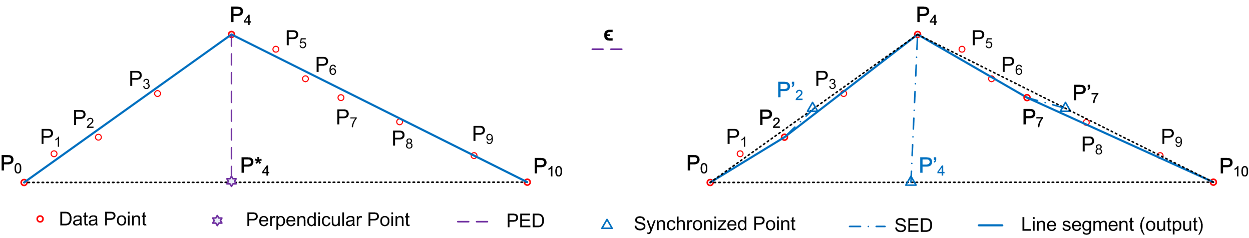
Figure 1: A trajectory $\dddot{\mathcal{T}}[P_{0},\ldots,P_{10}]$ with eleven points is represented by two (left) and four (right) continuous line segments (solid blue), compressed by the Douglas–Peucker algorithm Douglas:Peucker using $\mathsf{PED}$ and $\mathsf{SED}$, respectively. The Douglas–Peucker algorithm firstly creates line segment $\vv{P_{0}P_{10}}$, then it calculates the distance of each point in the trajectory to $\vv{P_{0}P_{10}}$. It finds that point $P_{4}$ has the maximum distance to $\vv{P_{0}P_{10}}$, and is greater than the user defined threshold $\epsilon$. Then it goes to compress sub-trajectories $[P_{0},\ldots,P_{4}]$ and $[P_{4},\ldots,P_{10}]$, separately.

Originally, line simplification ($\mathsf{LS}$) algorithms adopt the perpendicular Euclidean distance ($\mathsf{PED}$) as a metric to compute the errors, e.g., $|\vv{P_{4}P^{*}_{4}}|$ is the $\mathsf{PED}$ of data point $P_{4}$ to line segment $\vv{P_{0}P_{10}}$ in Figure 1 (left). Line simplification algorithms using $\mathsf{PED}$ have good compression ratios  Douglas:Peucker ; Hershberger:Speeding ; Lin:Operb ; Liu:BQS ; Muckell:Compression ; Chen:Trajectory ; Cao:Spatio ; Shi:Survey . However, when using $\mathsf{PED}$, the temporal information is lost. Thus, a spatio-temporal query, e.g., “the position of a moving object at time $t$”, on the compressed trajectories by $\mathsf{LS}$ algorithms using $\mathsf{PED}$ may return an approximate point $P^{\prime}$ whose distance to the actual position $P$ of the moving object at time $t$ is unbounded.

The synchronous Euclidean distance ($\mathsf{SED}$) was then introduced for trajectory compression to support the above spatio-temporal queries Meratnia:Spatiotemporal . $\mathsf{SED}$ is the Euclidean distance of a data point to its approximate temporally synchronized data point Meratnia:Spatiotemporal on the corresponding line segment. For instance, $P^{\prime}_{4}$ and $P^{\prime}_{7}$ are the synchronized data points of points $P_{4}$ and $P_{7}$ w.r.t. line segments $\vv{P_{0}P_{10}}$ and $\vv{P_{4}P_{10}}$, respectively, in Figure 1 (right). $\mathsf{LS}$ algorithms using $\mathsf{SED}$ may produce more line segments. However, the use of $\mathsf{SED}$ ensures that the Euclidean distance between a data point and its synchronized point w.r.t. the corresponding line segment is limited within a distance bound $\epsilon$. Hence, the above spatio-temporal query over the trajectories compressed by $\mathsf{SED}$ enabled approaches returns the synchronized point $P^{\prime}$ of a data point $P$ within the bound $\epsilon$.

The problem of finding the minimal number of line segments to represent the original polygonal lines w.r.t. an error bound $\epsilon$ is known as the “min-#” problemImai:Optimal ; Chan:Optimal . An optimal $O(n^{3})$ $\mathsf{LS}$ algorithm using $\mathsf{PED}$ was firstly developed in Imai:Optimal , where $n$ is the number of the original points. Later, an improved optimal $O(n^{2})$ algorithm using $\mathsf{PED}$ was designed in Chan:Optimal , with the help of sector intersection mechanism. However, the time complexity of the optimal $\mathsf{LS}$ algorithm using $\mathsf{SED}$ remains in $O(n^{3})$, as the optimization mechanisms are $\mathsf{PED}$ specific, and cannot work with $\mathsf{SED}$.

Due to the high time complexities of optimal $\mathsf{LS}$ algorithms using $\mathsf{SED}$, sub-optimal $\mathsf{LS}$ algorithms using $\mathsf{SED}$ have been developed for trajectory compression, including batch algorithms (e.g., Douglas-Peucker based algorithm $\mathsf{DPSED}$ Meratnia:Spatiotemporal ) and online algorithms (e.g., $\mathsf{SQUISH}$-$\mathsf{E}$ Muckell:Compression ). However, these methods still have high time and/or space complexities, which hinder their utilities in resource-constrained devices.

Observe that linear time $\mathsf{LS}$ algorithms using $\mathsf{PED}$ Williams:Longest ; Sklansky:Cone ; Dunham:Cone ; Zhao:Sleeve ; Lin:Operb have been develped, and they are more efficient for resource-constrained devices. The key idea to achieve a linear time complexity is by local distance checking in constant time, e.g., the sector intersection mechanism used in Williams:Longest ; Sklansky:Cone ; Dunham:Cone ; Zhao:Sleeve and the fitting function approach used in our preview work Lin:Operb . Unfortunately, these techinques are designed specifically for $\mathsf{PED}$, and cannot be applied for $\mathsf{SED}$.

Indeed, it is even more challenging to design an one-pass $\mathsf{LS}$ algorithm using $\mathsf{SED}$ than using $\mathsf{PED}$. To our knowledge, no one-pass $\mathsf{LS}$ algorithms using $\mathsf{SED}$ have been developed in the community.

Contributions. To this end, we propose two one-pass error bounded $\mathsf{LS}$ algorithms using $\mathsf{SED}$ for compressing trajectories in an efficient and effective way.

(1) We first develop a novel local synchronous distance checking approach, i.e., spatio-temporal Cone Intersection using the Synchronous Euclidean Distance (CISED). We further approximate the intersection of spatio-temporal cones with the intersection of regular polygons, and develop a fast regular polygon intersection algorithm, such that each data point in a trajectory is checked in $O(1)$ time during the entire process of trajectory simplification.

(2) We next develop two one-pass trajectory simplification algorithms $\mathsf{CISED}$-$\mathsf{S}$ and $\mathsf{CISED}$-$\mathsf{W}$, achieving $O(n)$ time complexity and $O(1)$ space complexity, based on our local synchronous distance checking technique. Algorithm $\mathsf{CISED}$-$\mathsf{S}$ belongs to strong simplification that only has original points in its outputs, while algorithm $\mathsf{CISED}$-$\mathsf{W}$ belongs to weak simplification that allows interpolated data points in its output.

(3) Using four real-life trajectory datasets ($\mathsf{Truck}$, $\mathsf{ServiceCar}$, $\mathsf{GeoLife}$, $\mathsf{PrivateCar}$), we finally conduct an extensive experimental study, by comparing our methods $\mathsf{CISED}$-$\mathsf{S}$ and $\mathsf{CISED}$-$\mathsf{W}$ with the optimal $\mathsf{LS}$ algorithm using $\mathsf{SED}$, $\mathsf{DPSED}$ Meratnia:Spatiotemporal (the most effective existing $\mathsf{LS}$ algorithm using $\mathsf{SED}$) and $\mathsf{SQUISH}$-$\mathsf{E}$ Muckell:Compression (the most efficient existing $\mathsf{LS}$ algorithm using $\mathsf{SED}$).

For running time, algorithms $\mathsf{CISED}$-$\mathsf{S}$ and $\mathsf{CISED}$-$\mathsf{W}$ are on average ($14.21$, $18.19$, $17.06$, $9.98$), ($2.84$, $3.45$, $3.69$, $2.86$) and ($925.25$, $7888.26$, $40041.59$, $8528.76$) times faster than $\mathsf{DPSED}$, $\mathsf{SQUISH}$-$\mathsf{E}$ and the optimal $\mathsf{LS}$ algorithm on datasets ($\mathsf{ServiceCar}$, $\mathsf{GeoLife}$, $\mathsf{Mopsi}$, $\mathsf{PrivateCar}$), respectively.

For compression ratios, algorithm $\mathsf{CISED}$-$\mathsf{S}$ is better than $\mathsf{SQUISH}$-$\mathsf{E}$ and comparable with $\mathsf{DPSED}$. The output sizes of $\mathsf{CISED}$-$\mathsf{S}$ are on average ($79.5\%$, $79.5\%$, $66.0\%$, $72.7\%$), ($109.1\%$, $109.7\%$, $113.5\%$, $109.2\%$) and ($134.3\%$, $133.3\%$, $148.4\%$, $135.4\%$) of $\mathsf{SQUISH}$-$\mathsf{E}$, $\mathsf{DPSED}$ and the optimal $\mathsf{LS}$ algorithm on datasets ($\mathsf{ServiceCar}$, $\mathsf{GeoLife}$, $\mathsf{Mopsi}$, $\mathsf{PrivateCar}$), respectively. Moreover, algorithm $\mathsf{CISED}$-$\mathsf{W}$ is comparable with the optimal $\mathsf{LS}$ algorithm and better than $\mathsf{SQUISH}$-$\mathsf{E}$ and $\mathsf{DPSED}$ that are on average ($57.9\%$, $58.8\%$, $48.4\%$, $54.6\%$), ($79.6\%$, $81.2\%$, $83.3\%$, $82.1\%$) and ($98.1\%$, $98.7\%$, $108.9\%$, $101.7\%$) of $\mathsf{SQUISH}$-$\mathsf{E}$, $\mathsf{DPSED}$ and the optimal $\mathsf{LS}$ algorithm on datasets ($\mathsf{ServiceCar}$, $\mathsf{GeoLife}$, $\mathsf{Mopsi}$, $\mathsf{PrivateCar}$), respectively.

Organization. The remainder of the article is organized as follows. Section 2 introduces the basic concepts and techniques. Section 3 presents our local synchronous distance checking method. Section 4 presents our one-pass trajectory simplification algorithms. Section 5 reports the experimental results, followed by related work in Section 6 and conclusion in Section 7.

2 Preliminaries

In this section, we first introduce basic concepts for piece-wise line based trajectory compression. We then describe the optimal $\mathsf{LS}$ algorithm and the sector intersection mechanism, and show how this mechanism can be used to fast the $\mathsf{LS}$ algorithms using $\mathsf{PED}$ and why it cannot work with $\mathsf{SED}$. Finally, we illustrate a convex polygon intersection algorithm, which serves as one of the fundamental components of our local synchronous distance checking method.

Notations used are summarized in Table 1.

2.1 Basic Notations

We first introduce basic notations.

Table 1: Summary of notations

Notations	Semantics
$P$	a data point
$\dddot{\mathcal{T}}$	a trajectory $\dddot{\mathcal{T}}$ is a sequence of data points
$\overline{\mathcal{T}}$	a piece-wise line representation of a
	trajectory $\dddot{\mathcal{T}}$
$\mathcal{L}$	a directed line segment
$ped(P,\mathcal{L})$	the perpendicular Euclidean distance of
	point $P$ to line segment $\mathcal{L}$
$sed(P,\mathcal{L})$	the synchronous Euclidean distance of
	point $P$ to line segment $\mathcal{L}$
$\epsilon$	the error bound
$\mathcal{S}{}$	a sector
$\vv{A}\times\vv{B}$	the cross product of (vectors) $\vv{A}$ and $\vv{B}$
$\mathcal{H}(\mathcal{L})$	The open half-plane to the left of $\mathcal{L}$
$\mathcal{R}$	a convex polygon
$\mathcal{R}^{*}$	the intersection of convex polygons
$m$	the maximum number of edges of a polygon
$E^{j}$	a group of edges labeled with $j$
$g(e)$	the label of an edge $e$ of polygons
$\mathcal{O}{}$	a synchronous circle
$\mathcal{C}{}$	a spatio-temporal cone
$\mathcal{O}^{c}{}$	a cone projection circle
$\bigsqcap$	intersection of geometries
$G$	the reachability graph of a trajectory

Points ($P$). A data point is defined as a triple $P(x,y,t)$, which represents that a moving object is located at longitude $x$ and latitude $y$ at time $t$. Note that data points can be viewed as points in a three-dimension Euclidean space.

Trajectories ($\dddot{\mathcal{T}}$). A trajectory $\dddot{\mathcal{T}}[P_{0},\ldots,P_{n}]$ is a sequence of data points in a monotonically increasing order of their associated time values (i.e., $P_{i}.t<P_{j}.t$ for any $0\leq i<j\leq n$). Intuitively, a trajectory is the path (or track) that a moving object follows through space as a function of time physics-trajectory .

Directed line segments ($\mathcal{L}$). A directed line segment (or line segment for simplicity) $\mathcal{L}$ is defined as $\vv{P_{s}P_{e}}$, which represents the closed line segment that connects the start point $P_{s}$ and the end point $P_{e}$. Note that here $P_{s}$ or $P_{e}$ may not be a point in a trajectory $\dddot{\mathcal{T}}$.

We also use $|\mathcal{L}|$ and $\mathcal{L}.\theta\in[0,2\pi)$ to denote the length of a directed line segment $\mathcal{L}$, and its angle with the $x$-axis of the coordinate system $(x,y)$, where $x$ and $y$ are the longitude and latitude, respectively. That is, a directed line segment $\mathcal{L}$ = $\vv{P_{s}P_{e}}$ can be treated as a triple $(P_{s},|\mathcal{L}|,\mathcal{L}.\theta)$.

Piecewise line representation ($\overline{\mathcal{T}}$). A piece-wise line representation $\overline{\mathcal{T}}[\mathcal{L}_{0},\ldots,\mathcal{L}_{m}]$ ($0<m\leq n$) of a trajectory $\dddot{\mathcal{T}}[P_{0},\ldots,P_{n}]$ is a sequence of continuous directed line segments $\mathcal{L}_{i}$ = $\vv{P_{s_{i}}P_{e_{i}}}$ ($i\in[0,m]$) of $\dddot{\mathcal{T}}$ such that $\mathcal{L}_{0}.P_{s_{0}}=P_{0}$, $\mathcal{L}_{m}.P_{e_{m}}=P_{n}$ and $\mathcal{L}_{i}.P_{e_{i}}$ = $\mathcal{L}_{i+1}.P_{s_{i+1}}$ for all $i\in[0,m-1]$. Note that each directed line segment in $\overline{\mathcal{T}}$ essentially represents a continuous sequence of data points in $\dddot{\mathcal{T}}$.

Perpendicular Euclidean Distance ($\mathsf{PED}$). Given a data point $P$ and a directed line segment $\mathcal{L}$ = $\vv{P_{s}P_{e}}$, the perpendicular Euclidean distance (or simply perpendicular distance) $ped(P,\mathcal{L})$ of point $P$ to line segment $\mathcal{L}$ is $\min\{|PQ|\}$ for any point $Q$ on $\vv{P_{s}P_{e}}$.

Synchronized points Meratnia:Spatiotemporal . Given a sub-trajectory $\dddot{\mathcal{T}}_{s}[P_{s}$, $\ldots,P_{e}]$, the synchronized point $P^{\prime}$ of a data point $P\in\dddot{\mathcal{T}}_{s}$, w.r.t. line segment $\vv{P_{s}P_{e}}$ is defined as follows: (1) $P^{\prime}.x$ = $P_{s}.x+c\cdot(P_{e}.x-P_{s}.x)$, (2) $P^{\prime}.y$ = $P_{s}.y+c\cdot(P_{e}.y-P_{s}.y)$ and (3) $P^{\prime}.t$ = $P.t$, where $c=\frac{P.t-P_{s}.t}{P_{e}.t-P_{s}.t}$.

Synchronous Euclidean Distance ($\mathsf{SED}$) Meratnia:Spatiotemporal . Given a data point $P$ and a directed line segment $\mathcal{L}$ = $\vv{P_{s}P_{e}}$, the synchronous Euclidean distance (or simply synchronous distance) $sed(P,\mathcal{L})$ of $P$ to $\mathcal{L}$ is $|\vv{PP^{\prime}}|$ that is the Euclidean distance from $P$ to its synchronized data point $P^{\prime}$ w.r.t. $\mathcal{L}$.

We illustrate these notations with examples.

Example 1

Consider Figure 1, in which

(1) $\dddot{\mathcal{T}}[P_{0}$, $\ldots,P_{10}]$ is a trajectory having 11 data points,

(2) the set of two continuous line segments $\{\vv{P_{0}P_{4}}$, $\vv{P_{4}P_{10}}$} (Left) and the set of four continuous line segments $\{\vv{P_{0}P_{2}}$, $\vv{P_{2}P_{4}}$, $\vv{P_{4}P_{7}}$, $\vv{P_{7}P_{10}}$} (Right) are two piecewise line representations of trajectory $\dddot{\mathcal{T}}$,

(3) $ped(P_{4},\vv{P_{0}P_{10}})=|\vv{P_{4}P^{*}_{4}}|$, where $P^{*}_{4}$ is the perpendicular point of $P_{4}$ w.r.t. line segment $\vv{P_{0}P_{10}}$, and

(4) $sed(P_{4},\vv{P_{0}P_{10}})=|\vv{P_{4}P^{\prime}_{4}}|$, $sed(P_{2},\vv{P_{0}P_{4}})=|\vv{P_{2}P^{\prime}_{2}}|$ and $sed(P_{7},\vv{P_{4}P_{10}})$ $=$ $|\vv{P_{7}P^{\prime}_{7}}|$, where points $P^{\prime}_{4}$, $P^{\prime}_{2}$ and $P^{\prime}_{7}$ are the synchronized points of $P_{4}$, $P_{2}$ and $P_{7}$ w.r.t. line segments $\vv{P_{0}P_{10}}$, $\vv{P_{0}P_{4}}$ and $\vv{P_{4}P_{10}}$, respectively. $\Box$

Error bounded algorithms. Given a trajectory $\dddot{\mathcal{T}}$ and its compression algorithm $\mathcal{A}$ using $\mathsf{SED}$ (respectively $\mathsf{PED}$) that produces another trajectory $\dddot{\mathcal{T^{\prime}}}$, we say that algorithm $\mathcal{A}$ is error bounded by $\epsilon$ if for each point $P$ in $\dddot{\mathcal{T}}$, there exist points $P_{j}$ and $P_{j+1}$ in $\dddot{\mathcal{T^{\prime}}}$ such that $sed(P,\mathcal{L}(P_{j},P_{j+1}))\leq\epsilon$ (respectively $ped(P,\mathcal{L}(P_{j},P_{j+1}))\leq\epsilon$).

2.2 The Optimal $\mathsf{LS}$ Algorithm

Given a trajectory $\dddot{\mathcal{T}}$${[P_{0},\ldots,P_{n}]}$ and an error bound $\epsilon$, the optimal trajectory simplification problem, as formulated by Imai and Iri in Imai:Optimal , can be solved in two steps: (1) construct a reachability graph $G$ of $\dddot{\mathcal{T}}$ and (2) search a shortest path from $P_{0}$ to $P_{n}$ in graph $G$.

The reachability graph of a trajectory $\dddot{\mathcal{T}}$${[P_{0},\ldots,P_{n}]}$ w.r.t. a bound $\epsilon$ is an unweighted graph $G(V,E)$, where (1) $V=\{P_{0},\ldots,P_{n}\}$, and (2) for any nodes $P_{s}$ and $P_{s+k}\in V$ ($s\geq 0,k>0,s+k\leq n$), edge $(P_{s},P_{s+k})\in E$ if and only if the distance of each point $P_{s+i}$ $(i\in[0,k])$ to line segment $\vv{P_{s}P_{s+k}}$ is no greater than $\epsilon$.

Observe that in the reachability graph $G$, (1) a path from nodes $P_{0}$ to $P_{n}$ is a representation of trajectory $\dddot{\mathcal{T}}$. The path also reveals the subset of points of $\dddot{\mathcal{T}}$ used in the approximate trajectory, (2) the path length corresponds to the number of line segments in the approximation trajectory, and (3) a shortest path is an optimal representation of trajectory $\dddot{\mathcal{T}}$.

Constructing the reachability graph $G$ needs to check for all pair of points $P_{s}$ and $P_{s+k}$ whether the distances of all points ($P_{s+i}$, $0<i<k$) to the line segment $\vv{P_{s}P_{s+k}}$ are less than $\epsilon$. There are $O(n^{2})$ pairs of points in the trajectory and checking the error of all points $P_{s+i}$ to a line segment $\vv{P_{s}P_{s+k}}$ takes $O(n)$ time. Thus, the construction step takes $O(n^{3})$ time. Finding shortest paths on unweighted graphs can be done in linear time. Hence, the brute-force algorithm takes $O(n^{3})$ time in total.

Though the brute-force algorithm was initially developed using $\mathsf{PED}$, it can be used for $\mathsf{SED}$. As pointed out in Chan:Optimal , the construction of the reachability graph $G$ using $\mathsf{PED}$ can be implemented in $O(n^{2})$ time using the sector intersection mechanism (see Section 2.3). However, the sector intersection mechanism cannot work with $\mathsf{SED}$. Hence, the construction of the reachability graph $G$ using $\mathsf{SED}$ remains in $O(n^{3})$ time, and the brute-force algorithm using $\mathsf{SED}$ remains in $O(n^{3})$ time.

2.3 Sector Intersection based Algorithms using $\mathsf{PED}$

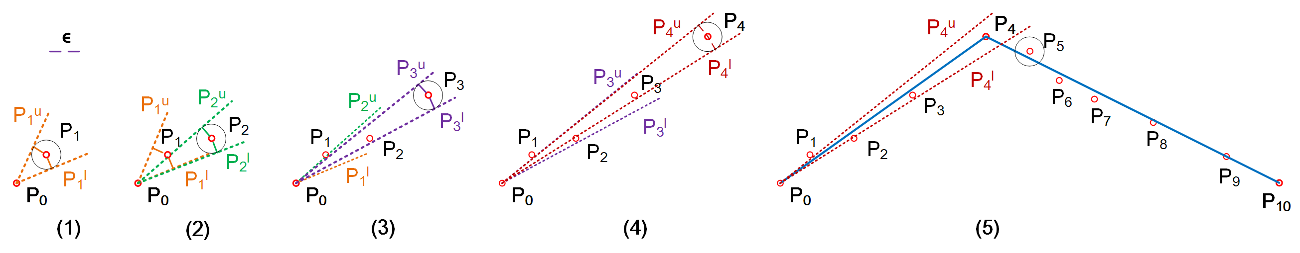
Figure 2: Trajectory $\dddot{\mathcal{T}}[P_{0},\ldots,P_{10}]$ in Figure 1 is compressed into two line segments by the Sector Intersection algorithm Williams:Longest ; Sklansky:Cone .

The sector intersection ($\mathsf{SI}$) algorithm Williams:Longest ; Sklansky:Cone was developed for graphic and pattern recognition in the late 1970s, for the approximation of arbitrary planar curves by linear segments or finding a polygonal approximation of a set of input data points in a 2D Cartesian coordinate system. The $\mathsf{Sleeve}$ algorithm Zhao:Sleeve in the cartographic discipline essentially applies the same idea as the $\mathsf{SI}$ algorithm. Further, Dunham:Cone optimized algorithm $\mathsf{SI}$ by considering the distance between a potential end point and the initial point of a line segment. It is worth pointing out that all these $\mathsf{SI}$ based algorithms use the perpendicular Euclidean distances.

Given a sequence of data points $[P_{s},P_{s+1},\ldots,P_{s+k}]$ and an error bound $\epsilon$, the $\mathsf{SI}$ based algorithms process the input points one by one in order, and produce a simplified polyline. Instead of using the distance threshold $\epsilon$ directly, the $\mathsf{SI}$ based algorithms convert the distance tolerance into a variable angle tolerance for testing the successive data points.

For the start data point $P_{s}$, any point $P_{s+i}$ and $|\vv{P_{s}P_{s+i}}|>\epsilon$ ($i\in[1,k]$), there are two directed lines $\vv{P_{s}P^{u}_{s+i}}$ and $\vv{P_{s}P^{l}_{s+i}}$ such that $ped(P_{s+i},\vv{P_{s}P^{u}_{s+i}})$ $=$ $ped(P_{s+i},\vv{P_{s}P^{l}_{s+i}})=\epsilon$ and either ($\vv{P_{s}P^{l}_{s+i}}.\theta<\vv{P_{s}P^{u}_{s+i}}.\theta\leavevmode\nobreak\ and\leavevmode\nobreak\ \vv{P_{s}P^{u}_{s+i}}.\theta-\vv{P_{s}P^{l}_{s+i}}.\theta<\pi$) or ($\vv{P_{s}P^{l}_{s+i}}.\theta>\vv{P_{s}P^{u}_{s+i}}.\theta\leavevmode\nobreak\ and\leavevmode\nobreak\ \vv{P_{s}P^{u}_{s+i}}.\theta-\vv{P_{s}P^{l}_{s+i}}.\theta<-\pi)$. Indeed, they forms a sector $\mathcal{S}{(P_{s},P_{s+i},\epsilon)}$ that takes $P_{s}$ as the center point and $\vv{P_{s}P^{u}_{s+i}}$ and $\vv{P_{s}P^{l}_{s+i}}$ as the border lines. Then there exists a data point $Q$ such that for any data point $P_{s+i}$ ($i\in[1,...k]$), its perpendicular Euclidean distance to directed line $\overline{P_{s}Q}$ is no greater than the error bound $\epsilon$ if and only if the $k$ sectors $\mathcal{S}{(P_{s},P_{s+i},\epsilon)}$ ($i\in[1,k]$) share common data points other than $P_{s}$, i.e., $\bigsqcap_{i=1}^{k}$$\mathcal{S}{(P_{s},P_{s+i},\epsilon)}$ $\neq\{P_{s}\}$ Williams:Longest ; Sklansky:Cone ; Zhao:Sleeve .

The point $Q$ may not belong to $\{P_{s},P_{s+1},$ $\ldots,P_{s+k}\}$. However, if $P_{s+i}$ ($1\leq i\leq k$) is chosen as $Q$, then for any data point $P_{s+j}$ ($j\in[1,...i]$), its perpendicular Euclidean distance to line segment $\overline{P_{s}P_{s+i}}$ is no greater than the error bound $\epsilon$ if and only if $\bigsqcap_{j=1}^{i}$$\mathcal{S}{(P_{s},P_{s+j},\epsilon/2)}$ $\neq\{P_{s}\}$, as pointed out in Zhao:Sleeve .

That is, these $\mathsf{SI}$ based algorithms can be easily adopted for trajectory compression using $\mathsf{PED}$ although they have been overlooked by existing trajectory simplification studies. The $\mathsf{SI}$ based algorithms run in $O(n)$ time and $O(1)$ space and are one-pass algorithms.

However, if we use $\mathsf{SED}$ instead of $\mathsf{PED}$, then “the $k$ sectors $\mathcal{S}{(P_{s},P_{s+i},\epsilon)}$ ($i\in[1,k]$) sharing common data points other than $P_{s}$” cannot ensure “there exists a data point $Q$ such that for any data point $P_{s+i}$ ($i\in[1,...k]$), its synchronized Euclidean distance to directed line $\overline{P_{s}Q}$ is no greater than the error bound $\epsilon$”. Hence, the $\mathsf{SI}$ mechanism is $\mathsf{PED}$ specific, and not applicable for $\mathsf{SED}$.

We next illustrate how the $\mathsf{SI}$ based algorithms can be used for trajectory compression with an example.

Example 2

Consider Figure 2. An $\mathsf{SI}$ based simplification algorithm takes as input a trajectory $\dddot{\mathcal{T}}[P_{0},\ldots,P_{10}]$, and returns a simplified ployline consisting of two line segments $\vv{P_{0}P_{4}}$ and $\vv{P_{4}P_{10}}$. Initially, point $P_{0}$ is the start point.

(1) Point $P_{1}$ is firstly read, and the sector $\mathcal{S}{(P_{0},P_{1},\epsilon/2)}$ of $P_{1}$ is created as shown in Figure 2.(1).

(2) Then $P_{2}$ is read, and the sector $\mathcal{S}{(P_{0},P_{2},\epsilon/2)}$ is created for $P_{2}$. The intersection of sectors $\mathcal{S}{(P_{0},P_{1},\epsilon/2)}$ and $\mathcal{S}{(P_{0},P_{2},\epsilon/2)}$ contains data points other than $P_{0}$, which has an up border line $P_{0}P_{2}^{u}$ and a low border line $P_{0}P_{1}^{l}$, as shown in Figure 2.(2).

Similarly, points $P_{3}$ and $P_{4}$ are processed, as shown in Figures 2.(3) and 2.(4), respectively.

(3) When point $P_{5}$ is read, line segment $\vv{P_{0}P_{4}}$ is produced, and point $P_{4}$ becomes the start point, as $\bigsqcap_{i=1}^{4}$$\mathcal{S}{(P_{0},P_{s+i},\epsilon/2)}$ $\neq\{P_{0}\}$ and $\bigsqcap_{i=1}^{5}$$\mathcal{S}{(P_{0},P_{s+i},\epsilon/2)}$ $=\{P_{0}\}$ as shown in Figure 2.(5).

(4) Points $P_{5},\ldots,P_{10}$ are processed similarly one by one in order, and finally the algorithm outputs another line segment $\vv{P_{4}P_{10}}$ as shown in Figure 2.(5). $\Box$

2.4 Intersection Computation of Convex Polygons

We also employ and revise a convex polygon intersection algorithm developed in ORourke:Intersection , whose basic idea is straightforward. Assume w.l.o.g. that the edges of polygons $\mathcal{R}_{1}$ and $\mathcal{R}_{2}$ are oriented counterclockwise, and $\vv{A}=(P_{s_{A}},P_{e_{A}})$ and $\vv{B}=(P_{s_{B}},P_{e_{B}})$ are two (directed) edges on $\mathcal{R}_{2}$ and $\mathcal{R}_{1}$, repectively (see Figure 4).

The algorithm has $\vv{A}$ and $\vv{B}$ “chasing” one another, i.e., moves $\vv{A}$ on $\mathcal{R}_{2}$ and $\vv{B}$ on $\mathcal{R}_{1}$ counter-clockwise step by step under certain rules, so that they meet at every crossing of $\mathcal{R}_{1}$ and $\mathcal{R}_{2}$. The rules, called advance rules, are carefully designed depending on geometric conditions of $\vv{A}$ and $\vv{B}$. Let $\vv{A}\times\vv{B}$ be the cross product of (vectors) $\vv{A}$ and $\vv{B}$, and $\mathcal{H}(\vv{A})$ be the open half-plane to the left of $\vv{A}$, the rules are as follows:

Rule (1): If $\vv{A}\times\vv{B}<0$ and $P_{e_{A}}\not\in\mathcal{H}(\vv{B})$, or $\vv{A}\times\vv{B}\geq 0$ and $P_{e_{B}}\in\mathcal{H}(\vv{A})$, then $\vv{A}$ is advanced a step.

For example, in Figure 4.(1) and 4.(2), $\vv{A}$ moves forward a step as $\vv{A}\times\vv{B}>0$ and $P_{e_{B}}\in\mathcal{H}(\vv{A})$.

Rule (2): If $\vv{A}\times\vv{B}\geq 0$ and $P_{e_{B}}\not\in\mathcal{H}(\vv{A})$, or $\vv{A}\times\vv{B}<0$ and $P_{e_{A}}\in\mathcal{H}(\vv{B})$, then $\vv{B}$ is advanced a step.

For example, in Figure 4.(6) and 4.(7), $\vv{B}$ moves forward a step as $\vv{A}\times\vv{B}<0$ and $P_{e_{A}}\in\mathcal{H}(\vv{B})$.

Algorithm $\mathsf{CPolyInter}$. The complete algorithm is shown in Figure 3. Given two convex polygons $\mathcal{R}_{1}$ and $\mathcal{R}_{2}$, algorithm $\mathsf{CPolyInter}$ first arbitrarily sets directed edge $\vv{A}$ on $\mathcal{R}_{2}$ and directed edge $\vv{B}$ on $\mathcal{R}_{1}$, respectively (line 1). It then checks the intersection of edges $\vv{A}$ and $\vv{B}$. If $\vv{A}$ intersects $\vv{B}$ (line 3), then the algorithm checks for some special termination conditions (e.g., if $\vv{A}$ and $\vv{B}$ are overlapped and, at the same time, polygons $\mathcal{R}_{1}$ and $\mathcal{R}_{2}$ are on the opposite sides of the overlapped edges, then the process is terminated) (line 4), and records the inner edge, which is a boundary segment of the intersection polygon (line 5). After that, the algorithm moves on $\vv{A}$ or $\vv{B}$ one step under the advance rules (lines 6–11). The above processes repeated, until both $\vv{A}$ and $\vv{B}$ cycle their polygons (line 12). Next, the algorithm handles three special cases of the polygons $\mathcal{R}_{1}$ and $\mathcal{R}_{2}$, i.e., $\mathcal{R}_{1}$ is inside of $\mathcal{R}_{2}$, $\mathcal{R}_{2}$ is inside of $\mathcal{R}_{1}$, and $\mathcal{R}_{1}\bigsqcap\mathcal{R}_{2}=\emptyset$ (line 13). At last, it returns the intersection polygon (line 14).

The algorithm has a time complexity of $O(|\mathcal{R}_{1}|+|\mathcal{R}_{2}|)$, where $|\mathcal{R}|$ is the number of edges of polygon $\mathcal{R}$. It is worth pointing out that $|\mathcal{R}_{1}\bigsqcap\mathcal{R}_{2}|\leq(|\mathcal{R}_{1}|+|\mathcal{R}_{2}|)$.

 

	Algorithm $\mathsf{CPolyInter}$ ($\mathcal{R}_{1}$, $\mathcal{R}_{2}$)
1.	set $\vv{A}$ and $\vv{B}$ arbitrarily on $\mathcal{R}_{2}$ and $\mathcal{R}_{1}$, respectively;
2.	repeat
3.	if $\vv{A}\bigsqcap\vv{B}\neq\emptyset$ then
4.	Check for termination;
5.	Update an inside flag;
6.	if ($\vv{A}\times\vv{B}<0$ and $P_{e_{A}}\not\in\mathcal{H}(\vv{B})$) or
7.	($\vv{A}\times\vv{B}\geq 0$ and $P_{e_{B}}\in\mathcal{H}(\vv{A})$) then
8.	advance $\vv{A}$ one step;
9.	elseif ($\vv{A}\times\vv{B}\geq 0$ and $P_{e_{B}}\not\in\mathcal{H}(\vv{A})$) or
10.	($\vv{A}\times\vv{B}<0$ and $P_{e_{A}}\in\mathcal{H}(\vv{B})$) then
11.	advance $\vv{B}$ one step;
12. until both $\vv{A}$ and $\vv{B}$ cycle their polygons
13. handle $\mathcal{R}_{1}\subset\mathcal{R}_{2}$ and $\mathcal{R}_{2}\subset\mathcal{R}_{1}$ and $\mathcal{R}_{1}\bigsqcap\mathcal{R}_{2}=\emptyset$ cases;
14. return $\mathcal{R}_{1}\bigsqcap\mathcal{R}_{2}$.

 

Figure 3: Algorithm for convex polygons intersection ORourke:Intersection .

Example 3

Figure 4 shows a running example of the convex polygon intersection algorithm $\mathsf{CPolyInter}$.

(1) Initially, directed edges $\vv{A}$ and $\vv{B}$ are on polygons $\mathcal{R}_{2}$ and $\mathcal{R}_{1}$, respectively, such that $\vv{A}\bigsqcap\vv{B}=\{P_{1}\}$, i.e., $\vv{A}$ and $\vv{B}$ intersect on point $P_{1}$, as shown in Figure 4.(1).

(2) Then, by advance rule (1), edge $\vv{A}$ moves on a step and makes $\vv{A}\bigsqcap\vv{B}=\emptyset$ as shown in Figure 4.(2). After 7 steps of moving of edge $\vv{A}$ or $\vv{B}$, each by an advance rule, $\vv{A}$ and $\vv{B}$ intersect on $P_{2}$, as shown in Figure 4.(6).

(3) Next, edge $\vv{B}$ moves on a step, and makes $\vv{A}\bigsqcap\vv{B}=\emptyset$, as shown in Figure 4.(7).

(4) After 6 steps of moving of edge $\vv{B}$ or $\vv{A}$ one by one, both edges $\vv{A}$ and $\vv{B}$ have finished their cycles as shown in Figure 4.(8).

(5) The algorithm finally returns the intersection polygon as shown in Figure 4.(9). $\Box$

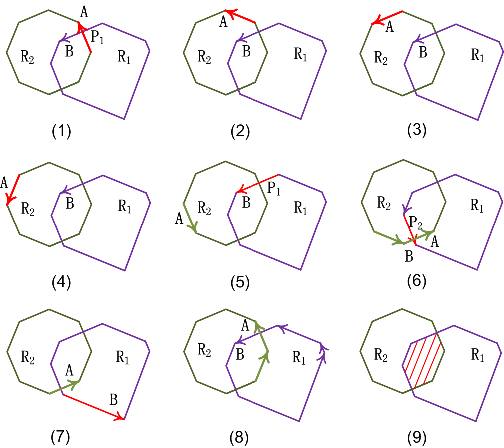
Figure 4: A running example of convex polygons intersection.

3 Local Synchronous Distance Checking

In this section, we develop a local synchronous distance checking approach such that each point in a trajectory is checked only once in $O(1)$ time during the entire process of trajectory simplification, by substantially extending the sector intersection method in Section 2.3 from a 2D space to a Spatio-Temporal 3D space, which lays down the key for the one-pass trajectory simplification algorithms using $\mathsf{SED}$ (Section 4).

We consider a sub-trajectory $\dddot{\mathcal{T}}_{s}[P_{s},\ldots,P_{s+k}]$, an error bound $\epsilon$, and a 3D Cartesian coordinate system whose origin, $x$-axis, $y$-axis and $t$-axis are $P_{s}$, longitude, latitude and time, respectively.

3.1 Spatio-Temporal Cone Intersection

We first present the spatio-temporal cone intersection method in a 3D Cartesian coordinate system, which extends the sector intersection method Williams:Longest ; Sklansky:Cone ; Zhao:Sleeve .

Synchronous Circles ($\mathcal{O}{}$). The synchronous circle of a data point $P_{s+i}$ ($1\leq i\leq k$) in $\dddot{\mathcal{T}}_{s}$ w.r.t. an error bound $\epsilon$, denoted as $\mathcal{O}{(P_{s+i},\epsilon)}$, or $\mathcal{O}{{}_{s+i}}$ in short, is a circle on the plane $P.t-P_{s+i}.t=0$ such that $P_{s+i}$ is its center and $\epsilon$ is its radius.

Figure 5 shows two synchronous circles, $\mathcal{O}{(P_{s+i},\epsilon)}$ of point $P_{s+i}$ and $\mathcal{O}{(P_{s+k},\epsilon)}$ of point $P_{s+k}$. It is easy to know that for any point in the area of a circle $\mathcal{O}{(P_{s+i},\epsilon)}$, its distance to $P_{s+i}$ is no greater than $\epsilon$.

Spatio-temporal cones ($\mathcal{C}{}$). The spatio-temporal cone (or simply cone) of a data point $P_{s+i}$ ($1\leq i\leq k$) in $\dddot{\mathcal{T}}_{s}$ w.r.t. a point $P_{s}$ and an error bound $\epsilon$, denoted as $\mathcal{C}{(P_{s},\mathcal{O}(P_{s+i},\epsilon))}$, or $\mathcal{C}{{}_{s+i}}$ in short, is an oblique circular cone such that point $P_{s}$ is its apex and the synchronous circle $\mathcal{O}(P_{s+i},\epsilon)$ of point $P_{s+i}$ is its base.

Figure 5 also illustrates two example spatio-temporal cones: $\mathcal{C}{(P_{s},\mathcal{O}(P_{s+i},\epsilon))}$ (purple) and $\mathcal{C}{(P_{s},\mathcal{O}(P_{s+k},\epsilon))}$ (red), with the same apex $P_{s}$ and error bound $\epsilon$.

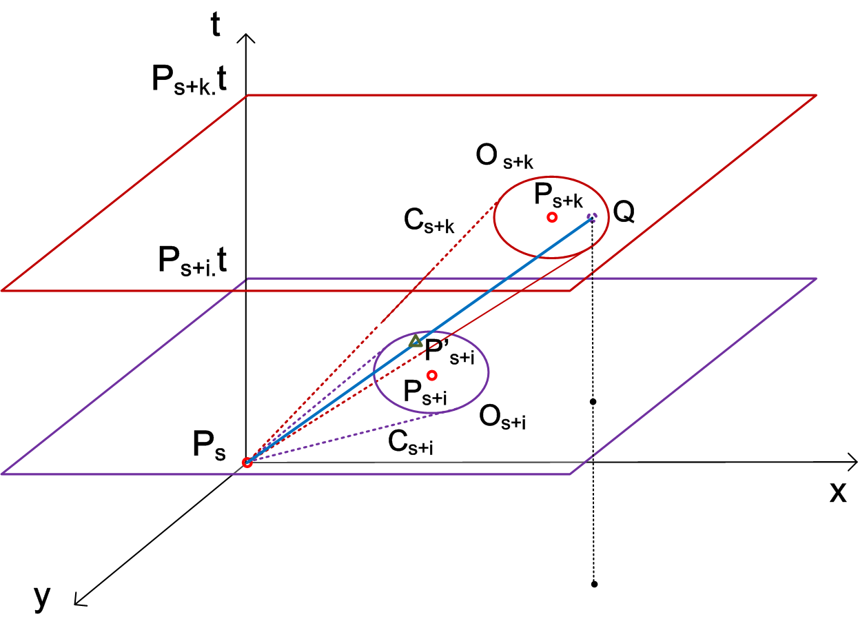
Figure 5: Examples of spatio-temporal cones in a 3D Cartesian coordinate system, where (1) $P_{s}$, $P_{s+i}$ and $P_{s+k}$ are three points, (2) $\mathcal{O}{{}_{s+i}}$ and $\mathcal{O}{{}_{s+k}}$ are two synchronous circles, (3) $\mathcal{C}{{}_{s+i}}$ and $\mathcal{C}{{}_{s+k}}$ are two spatio-temporal cones, (4) $Q$ is a point in synchronous circle $\mathcal{O}{{}_{s+k}}$, and (5) $P^{\prime}_{s+i}$ is the intersection point of line $\overline{P_{s}Q}$ and synchronous circle $\mathcal{O}{{}_{s+i}}$.

Proposition 1: Given a sub-trajectory $[P_{s},\ldots,P_{s+k}]$ and a point $Q$ in the area of synchronous circle $\mathcal{O}{(P_{s+k},\epsilon)}$, the intersection point $P^{\prime}_{s+i}$ of the directed line segment $\vv{P_{s}Q}$ and the plane $P.t-P_{s+i}.t=0$ is the synchronized point of $P_{s+i}$ ($1\leq i\leq k$) w.r.t. $\vv{P_{s}Q}$, and the distance $|\vv{P_{s+i}P^{\prime}_{s+i}}|$ from $P_{s+i}$ to $P^{\prime}_{s+i}$ is the synchronous distance of $P_{s+i}$ to $\vv{P_{s}Q}$. $\Box$

Proof

It suffices to show that $P^{\prime}_{s+i}$ is indeed a synchronized point $P_{s+i}$ w.r.t. $\vv{P_{s}Q}$. The intersection point $P^{\prime}_{s+i}$ satisfies that $P^{\prime}_{s+i}.t=P_{s+i}.t$ and $\frac{P^{\prime}_{s+i}.t-P_{s}.t}{Q.t-P_{s}.t}$ = $\frac{P_{s+i}.t-P_{s}.t}{Q.t-P_{s}.t}$ = $\frac{|\vv{P_{s}P^{\prime}_{s+i}}|}{|\vv{P_{s}Q}|}$ = $\frac{P^{\prime}_{s+i}.x-P_{s}.x}{Q.x-P_{s}.x}$ = $\frac{P^{\prime}_{s+i}.y-P_{s}.y}{Q.y-P_{s}.y}$. Hence, by the definition of synchronized points, we have the conclusion. $\Box$

Proposition 2: Given a sub-trajectory $[P_{s},...,P_{s+k}]$ and an error bound $\epsilon$, there exists a point $Q$ such that $Q.t=P_{s+k}.t$ and $sed(P_{s+i},\vv{P_{s}Q})\leq\epsilon$ for each $i\in[1,k]$ if and only if $\bigsqcap_{i=1}^{k}$$\mathcal{C}{(P_{s},\mathcal{O}(P_{s+i},\epsilon))}$ $\neq\{P_{s}\}$. $\Box$

Proof

Let $P^{\prime}_{s+i}$ ($i\in[1,k]$) be the intersection point of line segment $\vv{P_{s}Q}$ and the plane $P.t-P_{s+i}.t$ = $0$. By Proposition 5, $P^{\prime}_{s+i}$ is the synchronized point of $P_{s+i}$ w.r.t. $\vv{P_{s}Q}$.

Assume first that $\bigsqcap_{i=1}^{k}$$\mathcal{C}{(P_{s},\mathcal{O}(P_{s+i},\epsilon))}$ $\neq\{P_{s}\}$. Then there must exist a point $Q$ in the area of the synchronous circle $\mathcal{O}{(P_{s+k},\epsilon)}$ such that $\vv{P_{s}Q}$ passes through all the cones $\mathcal{C}{(P_{s},\mathcal{O}(P_{s+i},\epsilon))}$ $i\in[1,k]$. Hence, $Q.t=P_{s+k}.t$. We also have $sed(P_{s+i},\vv{P_{s}Q})=|\vv{P^{\prime}_{s+i}P_{s+i}}|\leq\epsilon$ for each $i\in[1,k]$ since $P^{\prime}_{s+i}$ is in the area of circle $\mathcal{O}{(P_{s+i},\epsilon)}$.

Conversely, assume that there exists a point $Q$ such that $Q.t=P_{s+k}.t$ and $sed(P_{s+i},\vv{P_{s}Q})\leq\epsilon$ for all $P_{s+i}$ ($i\in[1,k]$). Then $|\vv{P^{\prime}_{s+i}P_{s+i}}|\leq\epsilon$ for all $i\in[1,k]$. Hence, we have $\bigsqcap_{i=1}^{k}$$\mathcal{C}{(P_{s},\mathcal{O}(P_{s+i},\epsilon))}$ $\neq\{P_{s}\}$. $\Box$

By Proposition 3.1, we now have a spatio-temporal cone intersection method in a 3D Cartesian coordinate system, which significantly extends the sector intersection method Williams:Longest ; Sklansky:Cone ; Zhao:Sleeve from a 2D space to a Spatio-Temporal 3D space.

3.2 Circle Intersection

For spatio-temporal cones with the same apex $P_{s}$, the checking of their intersection can be computed by a much simpler way, i.e., the checking of intersection of cone projection circles on a plane, as follows.

Cone projection circles. The projection of a cone $\mathcal{C}{(P_{s},\mathcal{O}(P_{s+i},\epsilon))}$ on a plane $P.t-t_{c}=0$ ($t_{c}>P_{s}.t$) is a circle $\mathcal{O}^{c}{(P^{c}_{s+i},r^{c}_{s+i})}$, or $\mathcal{O}^{c}{{}_{s+i}}$ in short, such that (1) $P^{c}_{s+i}.x=P_{s}.x+c\cdot(P_{s+i}.x-P_{s}.x)$, (2) $P^{c}_{s+i}.y=P_{s}.y+c\cdot(P_{s+i}.y-P_{s}.y)$, (3) $P^{c}_{s+i}.t=t_{c}$ and (4) $r^{c}_{s+i}=c\cdot\epsilon$, where $c=\frac{t_{c}-P_{s}.t}{P_{s+i}.t-P_{s}.t}$ .

In Figure 6, the green dashed circles $\mathcal{O}^{c}{(P^{c}_{s+i},r^{c}_{s+i})}$ and $\mathcal{O}^{c}{(P^{c}_{s+k},r^{c}_{s+k})}$ on plane “$P.t-t_{c}=0$” are the projection circles of cones $\mathcal{C}{(P_{s},\mathcal{O}(P_{s+i},\epsilon))}$ and $\mathcal{C}{(P_{s},\mathcal{O}(P_{s+k},\epsilon))}$ on the plane.

Proposition 3: Given a sub-trajectory $[P_{s},\ldots,P_{s+k}]$, an error bound $\epsilon$, and any $t_{c}>P_{s}.t$, there exists a point $Q$ such that $Q.t=P_{s+k}.t$ and $sed(P_{s+i},\vv{P_{s}Q})\leq\epsilon$ for all points $P_{s+i}$ ($i\in[1,k]$) if and only if $\bigsqcap_{i=1}^{k}$$\mathcal{O}^{c}{(P^{c}_{s+i},r^{c}_{s+i})}$ $\neq\emptyset$. $\Box$

Proof

By Proposition 3.1, it suffices to show that $\bigsqcap_{i=1}^{k}$ $\mathcal{O}^{c}{(P^{c}_{s+i},r^{c}_{s+i})}$ $\neq\emptyset$ if and only if $\bigsqcap_{i=1}^{k}$$\mathcal{C}{(P_{s},\mathcal{O}(P_{s+i},\epsilon))}$$\neq\{P_{s}\}$, which is obvious. Hence, we have the conclusion. $\Box$

Proposition 3.2 tells us that the intersection checking of spatio-temporal cones can be reduced to simply check the intersection of cone projection circles on a plane.

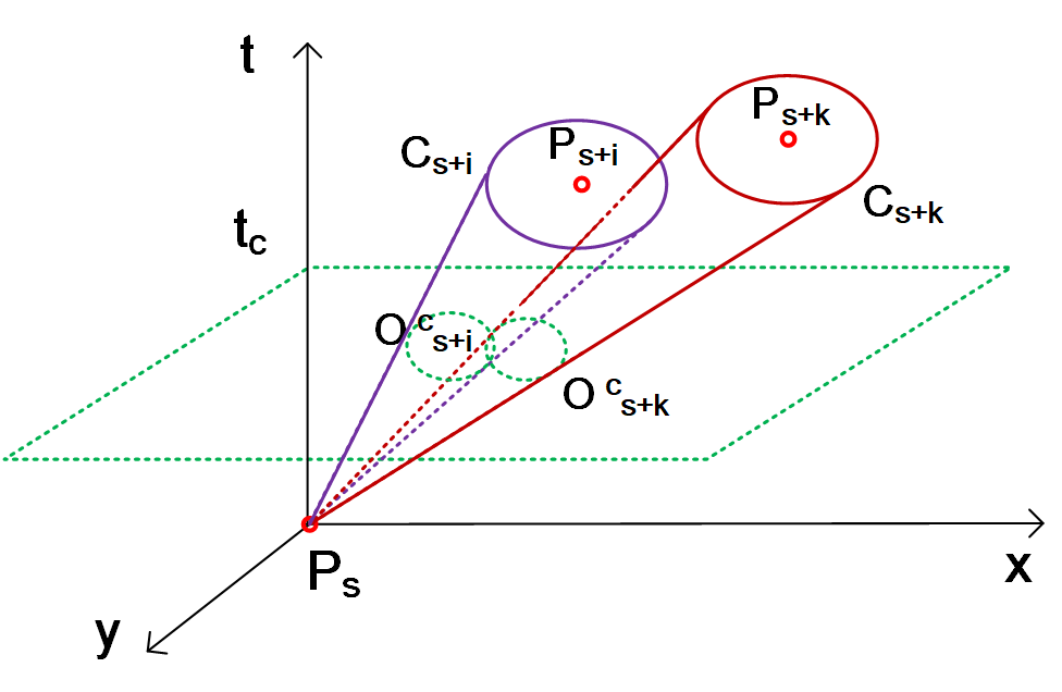
Figure 6: Cone projection circles.

3.3 Inscribed Regular Polygon Intersection

Finding the common intersection of $n$ circles on a plane has a time complexity of ${O(n\log n)}$ Shamos:Circle , which cannot be used for designing one-pass trajectory simplification algorithms using $\mathsf{SED}$. However, we can approximate a circle with its $m$-edge inscribed regular polygon, whose intersection can be computed more efficiently.

Inscribed regular polygons ($\mathcal{R}$). Given a cone projection circle $\mathcal{O}^{c}{(P,r)}$, its inscribed $m$-edge regular polygon is denoted as $\mathcal{R}(V,E)$, where (1) $V=\{v_{1},\ldots,v_{m}\}$ is the set of vertexes that are defined by a polar coordinate system, whose origin is the center $P$ of $\mathcal{O}^{c}{}$, as follows:

$$\hskip 21.52771ptv_{j}=(r,\frac{(j-1)}{m}2\pi),\leavevmode\nobreak\ j\in[1,m],$$

and (2) $E=\{\vv{v_{m}v_{1}}\}\bigcup\{\vv{v_{j}v_{j+1}}\ |\ j\in[1,m-1]\}$ is the set of edges that are labeled with the subscript of their start points.

Figure 7.(1) illustrates the inscribed regular octagon ($m=8$) of a cone projection circle $\mathcal{O}^{c}{(P,r)}$.

Let $\mathcal{R}_{s+i}$ ($1\leq i\leq k$) be the inscribed regular polygon of the cone projection circle $\mathcal{O}^{c}{(P^{c}_{s+i},r^{c}_{s+i})}$, $\mathcal{R}^{*}_{l}$ ($1\leq l\leq k$) be the intersection $\bigsqcap_{i=1}^{l}\mathcal{R}_{s+i}$, and $E^{j}$ ($1\leq j\leq m$) be the group of $k$ edges labeled with $j$ in all $\mathcal{R}_{s+i}$ ($i\in[1,k]$). It is easy to verify that all edges in the same edge groups $E^{j}$ ($1\leq j\leq m$) are in parallel (or overlapping) with each other by the above definition of inscribed regular polygons, as illustrated in Figure 7.(2).

Proposition 4: The intersection $\mathcal{R}^{*}_{l}\bigsqcap\mathcal{R}_{s+l+1}$ ($1\leq l<k$) has at most $m$ edges, i.e., at most one from each edge group. $\Box$

Proof

We shall prove this by contradiction. Assume that $\mathcal{R}^{*}_{l}\bigsqcap\mathcal{R}_{s+l+1}$ has two distinct edges $\vv{A_{i}}$ and $\vv{A_{i^{\prime}}}$ with the same label $j$ $(1\leq j\leq m)$, originally from $\mathcal{R}_{s+i}$ and $\mathcal{R}_{s+i^{\prime}}$ ($1\leq i<i^{\prime}\leq l+1$). Note that here $\mathcal{R}_{s+i}\bigsqcap\mathcal{R}_{s+i^{\prime}}\neq\emptyset$ since $\mathcal{R}^{*}_{l}\bigsqcap\mathcal{R}_{s+l+1}\neq\emptyset$. However, when $\mathcal{R}_{s+i}\bigsqcap\mathcal{R}_{s+i^{\prime}}\neq\emptyset$, the intersection $\mathcal{R}_{s+i}\bigsqcap\mathcal{R}_{s+i^{\prime}}$ cannot have both edge $\vv{A_{i}}$ and edge $\vv{A_{i^{\prime}}}$, which contradicts the assumption. $\Box$

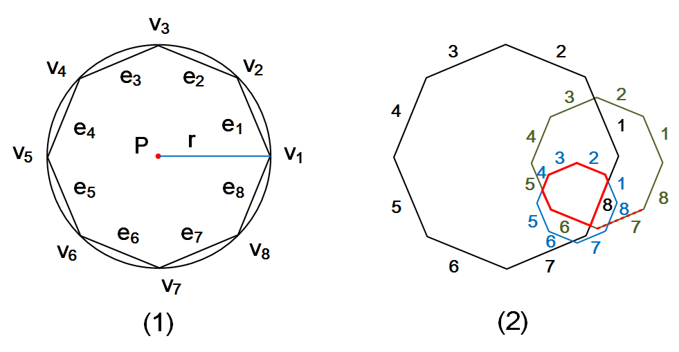
Figure 7: Regular octagons and their intersections ($m=8$).

Figure 7.(2) shows the intersection polygon (red lines) of $\mathcal{R}_{1}$, $\mathcal{R}_{2}$ and $\mathcal{R}_{3}$ with $7$ edges, and here edges labeled with $7$ have no contributions to the resulting intersection polygon.

Proposition 5: The intersection of $\mathcal{R}^{*}_{l}$ and $\mathcal{R}_{s+l+1}$ ($1\leq l<k$) can be done in $O(1)$ time. $\Box$

Proof

The inscribed regular polygon $\mathcal{R}_{s+l+1}$ has $m$ edges, and intersection polygon $\mathcal{R}^{*}_{l}$ has at most $m$ edges by Proposition 3.3. As the intersection of two $m$-edge convex polygons can be computed in $O(m)$ time ORourke:Intersection , the intersection of polygons $\mathcal{R}^{*}_{l}$ and $\mathcal{R}_{s+l+1}$ can be done in $O(1)$ time for a fixed $m$. $\Box$

3.4 Speedup Inscribed Regular Polygon Intersection

Observe that algorithm $\mathsf{CPolyInter}$ in Figure 3 is for general convex polygons, while the inscribed regular polygons $\mathcal{R}_{s+i}$ ($i\in[1,k]$) of the cone projection circles are constructed in a unified way, which allows us to develop a fast method to compute their intersection.

Let $\vv{A}=(P_{s_{A}},P_{e_{A}})$ and $\vv{B}=(P_{s_{B}},P_{e_{B}})$ be two directed edges on polygons $\mathcal{R}_{s+l+1}$ and $\mathcal{R}^{*}_{l}$, respectively. Again edges $\vv{A}$ and $\vv{B}$ are moved counter-clockwise. Note that $\vv{A}$ and $\vv{B}$ are advanced step by step each time by the two advancing rules of algorithm $\mathsf{CPolyInter}$. However, it is possible to advance $\vv{A}$ or $\vv{B}$ multiple steps each time. For example, in Figure 4.(1)–(5), edge $\vv{A}$ successively moves four steps, each under the advance rule (1) “($\vv{A}\times\vv{B}<0$ and $P_{e_{A}}\not\in\mathcal{H}(\vv{B})$) or ($\vv{A}\times\vv{B}\geq 0$ and $P_{e_{B}}\in\mathcal{H}(\vv{A})$)” of algorithm $\mathsf{CPolyInter}$. Alternatively, we can directly move $A$ from Figure 4.(1) to Figure 4.(5), by reducing four steps to one step only.

Proposition 6: If either $(\vv{A}\bigsqcap\vv{B}\neq\emptyset$ and $\vv{A}\times\vv{B}<0$ and $P_{e_{A}}\not\in\mathcal{H}(\vv{B}))$ or $(\vv{A}\bigsqcap\vv{B}\neq\emptyset$ and $\vv{A}\times\vv{B}\geq 0$ and $P_{e_{B}}\in\mathcal{H}(\vv{A}))$ holds, then $\vv{A}$ advances $s$ steps such that

$$\small\hskip 7.74997pts=\left\{\begin{aligned} &2\times(g(\vv{B})-g(\vv{A}))\hskip 19.37492pt\leavevmode\nobreak\ \leavevmode\nobreak\ if\leavevmode\nobreak\ g(\vv{B})>g(\vv{A})\\ &{1}\hskip 81.37468pt\leavevmode\nobreak\ if\leavevmode\nobreak\ g(\vv{A})=g(\vv{B})\\ &2\times(m+g(\vv{B})-g(\vv{A}))\leavevmode\nobreak\ \leavevmode\nobreak\ if\leavevmode\nobreak\ g(\vv{B})<g(\vv{A}),\\ \end{aligned}\right.\hskip 23.24991pt{}$$

in which $g(e)$ denotes the label of edge $e$. $\Box$

Proof

We first explain how the edge $\vv{A}$ advances. Indeed, $\vv{A}$ is moved from its original position to its symmetric edge on $\mathcal{R}_{s+l+1}$ w.r.t. the symmetric line that is perpendicular to $\vv{B}$ on $\mathcal{R}^{*}_{l}$. For example, in Figure 8.(1), there is $\vv{A}\bigsqcap\vv{B}\neq\emptyset$ and $\vv{A}\times\vv{B}\geq 0$ and $P_{e_{B}}\in\mathcal{H}(\vv{A})$, hence $\vv{A}$ moves on. As $g(\vv{B})=3>1=g(\vv{A})$, $\vv{A}$ moves forward $2\times(g(\vv{B})-g(\vv{A}))$ = $2\times(3-1)=4$ steps. Here, the label of edge $\vv{A}$ is changed to $5$, its symmetric edge $1$ on $\mathcal{R}_{s+l+1}$ w.r.t. the symmetric line that is perpendicular to $\vv{B}$ labeled with $3$ on $\mathcal{R}^{*}_{l}$.

We then present the proof. If ($\vv{A}\bigsqcap\vv{B}\neq\emptyset$ and $\vv{A}\times\vv{B}<0$ and $P_{e_{A}}\not\in\mathcal{H}(\vv{B})$) or ($\vv{A}\bigsqcap\vv{B}\neq\emptyset$ and $\vv{A}\times\vv{B}\geq 0$ and $P_{e_{B}}\in\mathcal{H}(\vv{A})$), then as all edges in the same edge groups $E^{j}$ ($1\leq j\leq m$) are in parallel with each other and by the geometric properties of regular polygon $\mathcal{R}_{s+k+1}$, it is easy to find that, for each position of $\vv{A}$ between its original to its opposite positions, we have (1) $\vv{A}\bigsqcap\vv{B}=\emptyset$, and (2) either $P_{e_{A}}\not\in\mathcal{H}(\vv{B})$ or $P_{e_{B}}\in\mathcal{H}(\vv{A})$. Hence, by the advance rule (1) of algorithm $\mathsf{CPolyInter}$ in Section 2.4, edge $\vv{A}$ is always moved forward until it reaches the opposite position of its original one. From this, we have the conclusion. $\Box$

Proposition 7: If either ($\vv{A}\bigsqcap\vv{B}\neq\emptyset$ and $\vv{A}\times\vv{B}\geq 0$ and $P_{e_{B}}\not\in\mathcal{H}(\vv{A})$) or ($\vv{A}\bigsqcap\vv{B}\neq\emptyset$ and $\vv{A}\times\vv{B}<0$ and $P_{e_{A}}\in\mathcal{H}(\vv{B})$) holds, then edge $\vv{B}$ is directly moved to the edge after the one having the same edge group as edge $\vv{A}$. $\Box$

Proof

We first explain how the edge $\vv{B}$ is moved forward. For example, in Figure 8.(2), $\vv{A}\bigsqcap\vv{B}\neq\emptyset$ and $\vv{A}\times\vv{B}<0$ and $P_{e_{A}}\in\mathcal{H}(\vv{B})$, hence $\vv{B}$ is moved forward. As the edge $\vv{A}$ is labeled with 7, $\vv{B}$ moves to the edge labeled with 8 on $\mathcal{R}^{*}_{l}$, which is the next of the edge labeled with 7 on $\mathcal{R}^{*}_{l}$. Note that if the edge labeled with 8 were not actually existing in the intersection polygon $\mathcal{R}^{*}_{l}$, then $\vv{B}$ should repeatedly move on until it reaches the first “real” edge on $\mathcal{R}^{*}_{l}$.

We then present the proof. If ($\vv{A}\bigsqcap\vv{B}\neq\emptyset$ and $\vv{A}\times\vv{B}\geq 0$ and $P_{e_{B}}\not\in\mathcal{H}(\vv{A})$) or ($\vv{A}\bigsqcap\vv{B}\neq\emptyset$ and $\vv{A}\times\vv{B}<0$ and $P_{e_{A}}\in\mathcal{H}(\vv{B})$), then it is also easy to find that, for each position of $\vv{B}$ between its original to its target positions (i.e., the edge after the one having the same edge group as $\vv{A}$), we have (1) $\vv{A}\bigsqcap\vv{B}=\emptyset$, and (2) either $P_{e_{B}}\not\in\mathcal{H}(\vv{A})$ or $P_{e_{A}}\in\mathcal{H}(\vv{B})$. Hence, by the advance rule (2) of algorithm $\mathsf{CPolyInter}$ in Section 2.4, edge $\vv{B}$ is always moved forward until it reaches the target position. From this, we have the conclusion. $\Box$

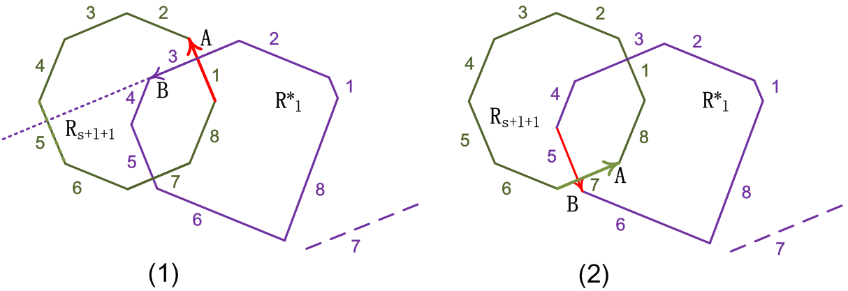
Figure 8: Examples of fast advancing rules.

Algorithm $\mathsf{FastRPolyInter}$. The presented regular polygon intersection algorithm, i.e., $\mathsf{FastRPolyInter}$, is the optimized version of the convex polygon intersection algorithm $\mathsf{CPolyInter}$, by Propositions 3.4 and 3.4. We also save vertexes of a polygon in a fixed size array, which is different from $\mathsf{CPolyInter}$ that saves polygons in linked lists. Considering the regular polygons each having a fixed number of vertexes/edges, marked from $1$ to $m$, this policy allows us to quickly address an edge or vertex by its label.

Given intersection polygon $\mathcal{R}^{*}_{l}$ of the preview $l$ polygons and the next approximate polygon $\mathcal{R}_{s+l+1}$, the algorithm $\mathsf{FastRPolyInter}$ returns $\mathcal{R}^{*}_{l+1}=\mathcal{R}^{*}_{l}\bigsqcap\mathcal{R}_{s+l+1}$. It runs the similar routine as the $\mathsf{CPolyInter}$ algorithm, except that (1) it saves polygons in arrays, and (2) the advance strategies are partitioned into two parts, i.e., $\vv{A}\bigsqcap\vv{B}\neq\emptyset$ and $\vv{A}\bigsqcap\vv{B}=\emptyset$, where the former applies Propositions 3.4 and 3.4, and the later remains the same as algorithm $\mathsf{CPolyInter}$.

Correctness and complexity analyses. Observe that algorithm $\mathsf{FastRPolyInter}$ basically has the same routine as algorithm $\mathsf{CPolyInter}$, except that it fastens the advancing speed of directed edges $\vv{A}$ and $\vv{B}$ under certain circumstances as shown by Propositions 3.4 and 3.4, which together ensure the correctness of $\mathsf{FastRPolyInter}$. Moreover, algorithm $\mathsf{FastRPolyInter}$ runs in $O(1)$ time by Proposition 7.

4 One-Pass Trajectory Simplification

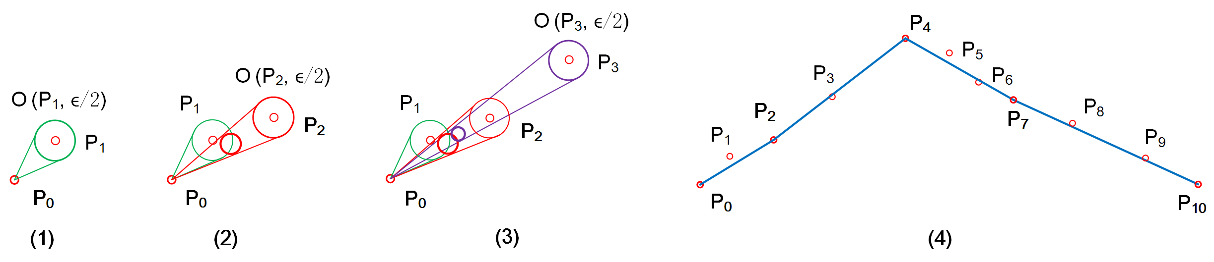
Figure 9: A running example of the $\mathsf{CISED}$-$\mathsf{S}$ algorithm. The points and the oblique circular cones are projected on an x-y space. The trajectory $\dddot{\mathcal{T}}[P_{0},\ldots,P_{10}]$ is compressed into four line segments.

Following Trajcevski:DDR ; Lin:Operb , we consider two classes of trajectory simplification. The first one, referred to as strong simplification, that takes as input a trajectory $\dddot{\mathcal{T}}$, an error bound $\epsilon$ and the number $m$ of edges for inscribed regular polygons, and produces a simplified trajectory $\dddot{\mathcal{T^{\prime}}}$ such that all data points in $\dddot{\mathcal{T^{\prime}}}$ belong to $\dddot{\mathcal{T}}$. The second one, referred to as weak simplification, that takes as input a trajectory $\dddot{\mathcal{T}}$, an error bound $\epsilon$ and the number $m$ of edges for inscribed regular polygons, and produces a simplified trajectory $\dddot{\mathcal{T^{\prime}}}$ such that some data points in $\dddot{\mathcal{T^{\prime}}}$ may not belong to $\dddot{\mathcal{T}}$. That is, weak simplification allows data interpolation.

The main result here is stated as follows.

Theorem 1

There exist one-pass, error bounded and strong and weak trajectory simplification algorithms using the synchronous Euclidean distance ($\mathsf{SED}$).

We shall prove this by providing such algorithms for both strong and weak trajectory simplifications, by employing the constant time synchronous distance checking technique developed in Section 3.

4.1 Strong Trajectory Simplification

Recall that in Propositions 3.1 and 3.2, the point $Q$ may not be in the input sub-trajectory $[P_{s},...,P_{s+k}]$. If we restrict $Q=P_{s+k}$, the end point of the sub-trajectory, then the narrow cones whose base circles with a radius of $\epsilon/2$ suffice.

Proposition 2: Given a sub-trajectory $[P_{s},...,P_{s+k}]$ and an error bound $\epsilon$, $sed(P_{s+i},\vv{P_{s}P_{s+k}})\leq\epsilon$ for each $i\in[1,k]$ if $\bigsqcap_{i=1}^{k}$$\mathcal{C}{(P_{s},\mathcal{O}(P_{s+i},\epsilon/2))}$ $\neq\{P_{s}\}$. $\Box$

Proof

If $\bigsqcap_{i=s+1}^{e}{\mathcal{C}(P_{s},P_{s+i},\epsilon/2)}\neq\{P_{s}\}$, then by Proposition 3.1, there exists a point $Q$, $Q.t=P_{s+k}.t$, such that $sed(P_{s+i},\vv{P_{s}Q})\leq\epsilon/2$ for all $i\in[1,k]$. By the triangle inequality essentially, $sed(P_{s+i},\vv{P_{s}P_{s+k}})\leq sed(P_{s+i},\vv{P_{s}Q})+|\vv{QP_{s+k}}|\leq\epsilon/2+\epsilon/2=\epsilon$. $\Box$

We first present the one-pass error bounded strong trajectory simplification algorithm using $\mathsf{SED}$, as shown in Figure 11.

Procedure $\mathsf{getRegularPolygon}$. We first present procedure $\mathsf{getRegularPolygon}$ that, given a cone projection circle, generates its inscribed $m$-edge regular polygon, following the definition in Section 3.3.

The parameters $P_{s}$, $P_{i}$, $r$ and $t_{c}$ together form the projection circle $\mathcal{O}^{c}{(P^{c}_{i},r^{c}_{i})}$ of the spatio-temporal cone $\mathcal{C}{(P_{s},\mathcal{O}(P_{i},r))}$ of point $P_{i}$ w.r.t. point $P_{s}$ on the plane $P.t-t_{c}$ = $0$. Firstly, $P^{c}_{i}.x$ and $P^{c}_{i}.y$ are computed (lines 1–3), and $r^{c}_{i}=c\cdot r$. Then it builds and returns an $m$-edge inscribed regular polygon $\mathcal{R}$ of $\mathcal{O}^{c}{(P^{c}_{i},r^{c}_{i})}$ (lines 4–8), by transforming a polar coordinate system into a Cartesian one. Note here $\theta$, $r\cdot\sin\theta$ and $r\cdot\cos\theta$ only need to be computed once during the entire processing of a trajectory.

Algorithm $\mathsf{CISED}$-$\mathsf{S}$. It takes as input a trajectory $\dddot{\mathcal{T}}$${[P_{0},\ldots,P_{n}]}$, an error bound $\epsilon$ and the number $m$ of edges for inscribed regular polygons, and returns a simplified trajectory $\overline{\mathcal{T}}$ of $\dddot{\mathcal{T}}$.

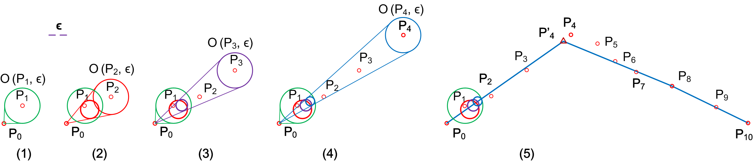
Figure 10: A running example of the $\mathsf{CISED}$-$\mathsf{W}$ algorithm. The points and the oblique circular cones are projected on an x-y space. The trajectory $\dddot{\mathcal{T}}[P_{0},\ldots,P_{10}]$ is compressed into three line segments.

The algorithm first initializes the start point $P_{s}$ to $P_{0}$, the index $i$ of the current data point to $1$, the intersection polygon $\mathcal{R}^{*}$ to $\emptyset$, the output $\overline{\mathcal{T}}$ to $\emptyset$, and $t_{c}$ to $P_{1}.t$, respectively (line 1). The algorithm sequentially processes the data points of the trajectory one by one (lines 2–10). It gets the $m$-inscribed regular polygon w.r.t. the current point $P_{i}$ (line 3) by calling procedure ${\mathsf{getRegularPolygon}}$. When $\mathcal{R}^{*}=\emptyset$, the intersection polygon $\mathcal{R}^{*}$ is simply initialized as $\mathcal{R}$ (lines 4, 5). Otherwise, $\mathcal{R}^{*}$ is the intersection of the current regular polygon $\mathcal{R}$ with $\mathcal{R}^{*}$ by calling procedure ${\mathsf{FastRPolyInter}}()$ introduced in Section 3.4 (line 7). If the resulting intersection $\mathcal{R}^{*}$ is empty, then a new line segment $\vv{P_{s}P_{i-1}}$ is generated (lines 8–10). The process repeats until all points have been processed (line 11). After the final new line segment $\vv{P_{s}P_{n}}$ is generated (line 12), it returns the simplified piece-wise line representation $\overline{\mathcal{T}}$ (line 13).

 

		Algorithm $\mathsf{CISED}$-$\mathsf{S}$ $(\dddot{\mathcal{T}}[P_{0},\ldots,P_{n}],\leavevmode\nobreak\ \epsilon,\leavevmode\nobreak\ m)$
1.	$P_{s}:=P_{0}$;  $i:=1$;  $\mathcal{R}^{*}:=\emptyset$;  $\overline{\mathcal{T}}:=\emptyset$;  $t_{c}$ := $P_{1}.t$;
2.	while $i\leq n$ do
3.	$\mathcal{R}$ := $\mathsf{getRegularPolygon}$ ($P_{s}$, $P_{i}$, $\epsilon/2$, $m$, $t_{c}$);
4.	if $\mathcal{R}^{*}=\emptyset$ then      /* $\mathcal{R}^{*}$ needs to be initialized */
5.	$\mathcal{R}^{*}:=\mathcal{R};$
6.	else
7.	$\mathcal{R}^{*}:={{\mathsf{FastRPolyInter}}}(\mathcal{R}^{*},\leavevmode\nobreak\ \mathcal{R})$;
8.	if $\mathcal{R}^{*}=\emptyset$ then    /* generate a new line segment */
9.	$i$ := $i-1$;  $\overline{\mathcal{T}}:=\overline{\mathcal{T}}\cup\{\vv{P_{s}P_{i}}\}$;
10.	$P_{s}:=P_{i}$;   $t_{c}$ := $P_{i+1}.t$;
11.	$i$ := $i+1$;
12.	$\overline{\mathcal{T}}$ := $\overline{\mathcal{T}}\cup\{\vv{P_{s}P_{n}}\}$;
13.  return $\overline{\mathcal{T}}$.
Procedure  $\mathsf{getRegularPolygon}$ $(P_{s},\leavevmode\nobreak\ P_{i},\leavevmode\nobreak\ r,\leavevmode\nobreak\ m,\leavevmode\nobreak\ t_{c})$
1.   $c:=(t_{c}-t_{s})/(P_{i}.t-P_{s}.t)$;
2.   $x:=P_{s}.x+c\cdot(P_{i}.x-P_{s}.x)$;
3.   $y:=P_{s}.y+c\cdot(P_{i}.y-P_{s}.y)$;
4.   for $(j:=1;j\leq m;j++)$ do
5.	$\theta:=(2j+1)*\pi/m$;
6.	$\mathcal{R}.v_{j}.x:=x+c\cdot r\cdot\cos\theta$;
7.	$\mathcal{R}.v_{j}.y:=y+c\cdot r\cdot\sin\theta$;
8.   return $\mathcal{R}$.

 

Figure 11: One-pass strong trajectory simplification algorithm.

Example 4

Figure 9 shows a running example of $\mathsf{CISED}$-$\mathsf{S}$ for compressing the trajectory $\dddot{\mathcal{T}}$ in Figure 1.

(1) After initialization, the $\mathsf{CISED}$-$\mathsf{S}$ algorithm reads point $P_{1}$ and builds a narrow oblique circular cone $\mathcal{C}{(P_{0},\mathcal{O}(P_{1},\epsilon/2))}$, taking $P_{0}$ as its apex and $\mathcal{O}{(P_{1},\epsilon/2)}$ as its base (green dash). The circular cone is projected on the plane $P.t-P_{1}.t=0$, and the inscribe regular polygon $\mathcal{R}_{1}$ of the projection circle is returned. As $\mathcal{R}^{*}$ is empty, $\mathcal{R}^{*}$ is set to $\mathcal{R}_{1}$.

(2) The algorithm reads $P_{2}$ and builds $\mathcal{C}{(P_{0},\mathcal{O}(P_{2},\epsilon/2))}$ (red dash). The circular cone is also projected on the plane $P.t-P_{1}.t=0$ and the inscribe regular polygon $\mathcal{R}_{2}$ of the projection circle is returned. As $\mathcal{R}^{*}=\mathcal{R}_{1}$ is not empty, $\mathcal{R}^{*}$ is set to the intersection of $\mathcal{R}_{2}$ and $\mathcal{R}^{*}$, which is $\mathcal{R}_{1}\bigsqcap\mathcal{R}_{2}\neq\emptyset$.

(3) For point $P_{3}$, the algorithm runs the same routine as $P_{2}$ until the intersection of $\mathcal{R}_{3}$ and $\mathcal{R}^{*}$ is $\emptyset$. Thus, a line segment $\vv{P_{0}P_{2}}$ is generated, and the process of a new line segment is started, taking $P_{2}$ as the new start point and $P.t-P_{3}.t=0$ as the new projection plane.

(4) At last, the algorithm outputs four continuous line segments, i.e., $\{\vv{P_{0}P_{2}}$, $\vv{P_{2}P_{4}}$, $\vv{P_{4}P_{7}}$, $\vv{P_{7}P_{10}}\}$. $\Box$

4.2 Weak Trajectory Simplification

We then present the one-pass error bounded weak simplification algorithm using $\mathsf{SED}$.

Algorithm $\mathsf{CISED}$-$\mathsf{W}$. Given a trajectory $\dddot{\mathcal{T}}$${[P_{0},\ldots,P_{n}]}$, an error bound $\epsilon$ and the number $m$ of edges for inscribed regular polygons, it returns a simplified trajectory, which may contain interpolated points. By Proposition 3.2, algorithm $\mathsf{CISED}$-$\mathsf{W}$ generates spatio-temporal cones whose bases are circles with a radius of $\epsilon$, and, hence, it replaces $\epsilon/2$ with $\epsilon$ (line 3 of $\mathsf{CISED}$-$\mathsf{S}$). It also generates new line segments with data points $Q$ (may be interpolated points), and, hence, it replaces point $P_{i}$ and line segment $\vv{P_{s}P_{i}}$ (lines 9 and 10 of algorithm $\mathsf{CISED}$-$\mathsf{S}$) with $Q$ and $\vv{P_{s}Q}$, respectively, such that $Q$ is generated as follows.

Proposition 3: Given a sub-trajectory $\dddot{\mathcal{T}}$${[P_{s},\ldots,P_{s+k}]}$ and an error bound $\epsilon$, $t_{c}=P_{s+k}.t$ and $\mathcal{R}^{*}_{k}$ be the intersection of all polygons $\mathcal{R}_{s+i}$ ($i\in[1,k]$) on the plane $P.t-t_{c}=0$. If $\mathcal{R}^{*}_{k}$ is not empty, then any point in the area of $\mathcal{R}^{*}_{k}$ is feasible for $Q$. $\Box$

Proof

By Proposition 3.2 and the nature of inscribed regular polygon, it is easy to find that for any point $Q\in\mathcal{R}^{*}_{k}$ w.r.t. plane $t_{c}=P_{s+k}.t$, there is $sed(P_{s+i},\vv{P_{s}Q})\leq\epsilon$ for all points $P_{s+i}$ ($i\in[1,k]$).

From this, we have the conclusion. $\Box$

The choice of a point $Q$ from $\mathcal{R}^{*}_{k}$ may slightly affect the effectiveness (e.g., average errors and compression ratios). However, the choice of an optimal $Q$ is non-trivial. For the benefit of efficiency, we apply the following strategies.

(1) If $P_{s+k}$ is in the area of $\mathcal{R}^{*}_{k}$ w.r.t. $t_{c}=P_{s+k}.t$, then $Q$ is simply chosen as $P_{s+k}$.

(2) If $\mathcal{R}^{*}_{k}\neq\emptyset$ and $P_{s+k}$ is not in the area of $\mathcal{R}^{*}_{k}$ w.r.t. $t_{c}$=$P_{s+k}.t$, then the central point of $\mathcal{R}^{*}_{k}$ is chosen as $Q$.

(3) If $t_{c}\neq P_{s+k}.t$, which is the general case, then we project the intersection polygon $\mathcal{R}^{*}_{k}$ w.r.t. $t_{c}\neq P_{s+k}.t$ on the plane $P.t-P_{s+k}.t=0$, and apply strategies (1) and (2) above. That is, the projection has no affects on the choice of $Q$.

Example 5

Figure 10 shows a running example of algorithm $\mathsf{CISED}$-$\mathsf{W}$ for compressing the trajectory $\dddot{\mathcal{T}}$ in Figure 1 again.

(1) After initialization, the $\mathsf{CISED}$-$\mathsf{W}$ algorithm reads point $P_{1}$ and builds an oblique circular cone $\mathcal{C}{(P_{0},\mathcal{O}(P_{1},\epsilon))}$, and projects it on the plane $P.t-P_{1}.t=0$. The inscribed regular polygon $\mathcal{R}_{1}$ of the projection circle is returned and the intersection $\mathcal{R}^{*}$ is set to $\mathcal{R}_{1}$.

(2) $P_{2}$, $P_{3}$ and $P_{4}$ are processed in turn. The intersection polygons $\mathcal{R}^{*}$ are not empty.

(3) For point $P_{5}$, the intersection of polygons $\mathcal{R}_{5}$ and $\mathcal{R}^{*}$ is $\emptyset$. Thus, line segment $\vv{P_{0}Q}=\vv{P_{0}P^{\prime}_{4}}$ is output, and a new line segment is started such that point $Q=P^{\prime}_{4}$ is the new start point and plane $P.t-P_{5}.t=0$ is the new projection plane.

(4) At last, the algorithm outputs 3 continuous line segments, i.e., $\vv{P_{0}P^{\prime}_{4}}$, $\vv{P^{\prime}_{4}P_{8}}$ and $\vv{P_{8}P_{10}}$, in which $P^{\prime}_{4}$ is an interpolated data points not in $\dddot{\mathcal{T}}$. $\Box$

Table 2: Real-life trajectory datasets

Data Sets	Number of Trajectories	Sampling Rates (s)	Points Per Trajectory (K)	Total points
$\mathsf{ServiceCar}$	1,000	3-5	$\sim 114.0$	114M
$\mathsf{GeoLife}$	182	1-5	$\sim 131.4$	24.2M
$\mathsf{Mopsi}$	51	2	$\sim 153.9$	7.9M
$\mathsf{PrivateCar}$	10	1	$\sim 11.8$	112.8K

Correctness and complexity analyses. The correctness of algorithms $\mathsf{CISED}$-$\mathsf{S}$ and $\mathsf{CISED}$-$\mathsf{W}$ follows from Propositions 3.2 and 4.1, and Propositions 3.2 and 4.2, respectively. It is easy to verify that each data point in a trajectory is only processed once, and each can be done in $O(1)$ time, as both procedures ${\mathsf{getRegularPolygon}}$ and ${\mathsf{FastRPolyInter}}$ can be done in $O(1)$ time. Hence, these algorithms are both one-pass error bounded trajectory simplification algorithms. It is also easy to see that these algorithms take $O(1)$ space.

5 Experimental Study

In this section, we present an extensive experimental study of our one-pass trajectory simplification algorithms ($\mathsf{CISED}$-$\mathsf{S}$ and $\mathsf{CISED}$-$\mathsf{W}$) compared with the optimal algorithm using $\mathsf{SED}$ and existing algorithms of $\mathsf{DPSED}$ and $\mathsf{SQUISH}$-$\mathsf{E}$ on trajectory datasets. Using four real-life trajectory datasets, we conducted three sets of experiments to evaluate: (1) the compression ratios of algorithms $\mathsf{CISED}$-$\mathsf{S}$ and $\mathsf{CISED}$-$\mathsf{W}$ vs. $\mathsf{DPSED}$, $\mathsf{SQUISH}$-$\mathsf{E}$ and the optimal algorithm, (2) the average errors of algorithms $\mathsf{CISED}$-$\mathsf{S}$ and $\mathsf{CISED}$-$\mathsf{W}$ vs. $\mathsf{DPSED}$, $\mathsf{SQUISH}$-$\mathsf{E}$ and the optimal algorithm, (3) the execution time of algorithms $\mathsf{CISED}$-$\mathsf{S}$ and $\mathsf{CISED}$-$\mathsf{W}$ vs. $\mathsf{DPSED}$, $\mathsf{SQUISH}$-$\mathsf{E}$ and the optimal algorithm, and (4) the impacts of polygon intersection algorithms $\mathsf{FastRPolyInter}$ and $\mathsf{CPolyInter}$ and the edge number $m$ of inscribed regular polygons to the effectiveness and efficiency of algorithms $\mathsf{CISED}$-$\mathsf{S}$ and $\mathsf{CISED}$-$\mathsf{W}$.

5.1 Experimental Setting

Real-life Trajectory Datasets. We use four real-life datasets $\mathsf{ServiceCar}$, $\mathsf{GeoLife}$, $\mathsf{Mopsi}$ and $\mathsf{PrivateCar}$ shown in Table 2 to test our solutions.

(1) Service car trajectory data ($\mathsf{ServiceCar}$) is the GPS trajectories collected by a Chinese car rental company during Apr. 2015 to Nov. 2015. The sampling rate was one point per $3$–$5$ seconds, and each trajectory has around $114.1K$ points.

(2) GeoLife trajectory data ($\mathsf{GeoLife}$) is the GPS trajectories collected in GeoLife project Zheng:GeoLife by 182 users in a period from Apr. 2007 to Oct. 2011. These trajectories have a variety of sampling rates, among which 91% are logged in each 1-5 seconds per point.

(3) Mopsi trajectory data ($\mathsf{Mopsi}$) is the GPS trajectories collected in Mopsi project Mopsi by 51 users in a period from 2008 to 2014. Most routes are in Joensuu region, Finland. The sampling rate was one point per $2$ seconds, and each trajectory has around $153.9K$ points.

(4) Private car trajectory data ($\mathsf{PrivateCar}$) is a small set GPS trajectories collected with a high sampling rate of one point per second by our team members in 2017. There are 10 trajectories and each trajectory has around 11.8K points.

(5) Small trajectory data. As the optimal $\mathsf{LS}$ algorithm Imai:Optimal it has both high time and space complexities, i.e., $O(n^{3})$ time and $O(n^{2})$ space, it is impossible to compress the entire datasets (too slow and out of memory). Hence, we further build four small datasets, each dataset includes 10 middle-size ($10K$ points per trajectory) trajectories selected from $\mathsf{ServiceCar}$, $\mathsf{GeoLife}$, $\mathsf{Mopsi}$ and $\mathsf{PrivateCar}$, respectively.

Algorithms and implementation. We implement five $\mathsf{LS}$ algorithms, i.e., our $\mathsf{CISED}$-$\mathsf{S}$ and $\mathsf{CISED}$-$\mathsf{W}$, $\mathsf{DPSED}$ Meratnia:Spatiotemporal (the most effective existing $\mathsf{LS}$ algorithm using $\mathsf{SED}$), $\mathsf{SQUISH}$-$\mathsf{E}$ Muckell:Compression (the most efficient existing $\mathsf{LS}$ algorithm using $\mathsf{SED}$) and the optimal $\mathsf{LS}$ algorithm using $\mathsf{SED}$ (see Section 2.2). We also implement the polygon intersection algorithms, $\mathsf{CPolyInter}$ and our $\mathsf{FastRPolyInter}$. All algorithms were implemented with Java. All tests were run on an x64-based PC with 8 Intel(R) Core(TM) i7-6700 CPU @ 3.40GHz and 8GB of memory, and each test was repeated over 3 times and the average is reported here.

5.2 Experimental Results

We next present our findings.

5.2.1 Evaluation of Compression Ratios

In the first set of tests, we evaluate the impacts of parameter $m$ on the compression ratios of our algorithms $\mathsf{CISED}$-$\mathsf{S}$ and $\mathsf{CISED}$-$\mathsf{W}$, and compare the compression ratios of $\mathsf{CISED}$-$\mathsf{S}$ and $\mathsf{CISED}$-$\mathsf{W}$ with $\mathsf{DPSED}$, $\mathsf{SQUISH}$-$\mathsf{E}$ and the optimal algorithm. The compression ratio is defined as follows: Given a set of trajectories $\{\dddot{\mathcal{T}_{1}},\ldots,\dddot{\mathcal{T}_{M}}\}$ and their piecewise line representations $\{\overline{\mathcal{T}_{1}},\ldots,\overline{\mathcal{T}_{M}}\}$, the compression ratio of an algorithm is $(\sum_{j=1}^{M}|\overline{\mathcal{T}}_{j}|)/(\sum_{j=1}^{M}|\dddot{\mathcal{T}}_{j}|)$. By the definition, algorithms with lower compression ratios are better.

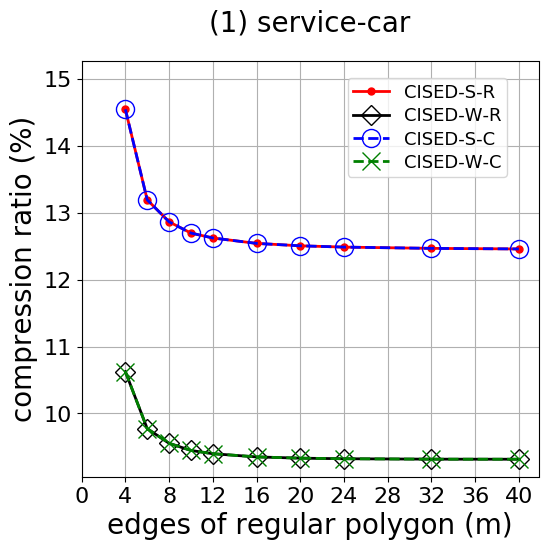
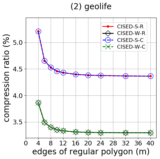
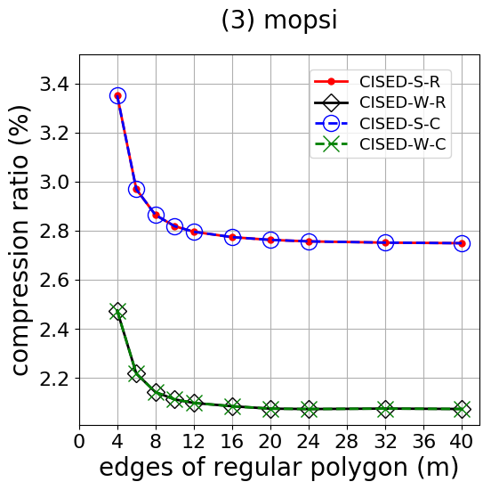
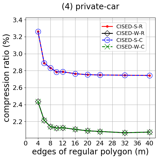
Figure 12: Evaluation of compression ratios: fixed error bound with $\epsilon=60$ meters and varying $m$.

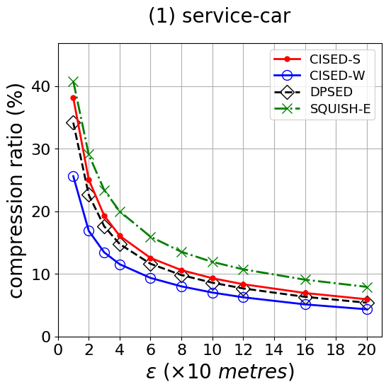
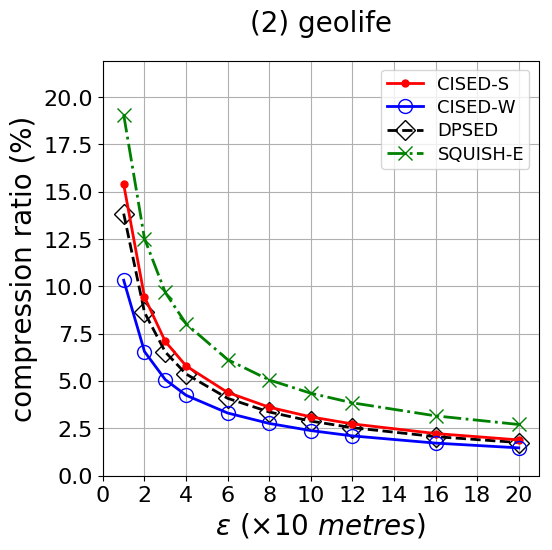
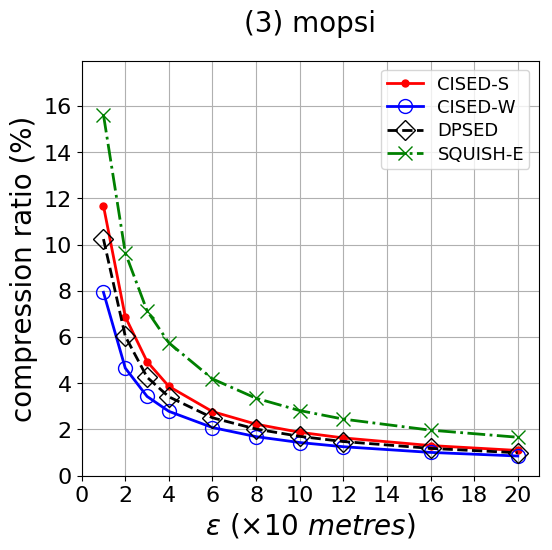
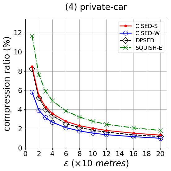
Figure 13: Evaluation of compression ratios: fixed with $m=16$ and varying error bound $\epsilon$.

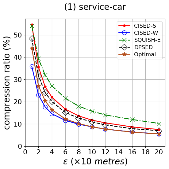
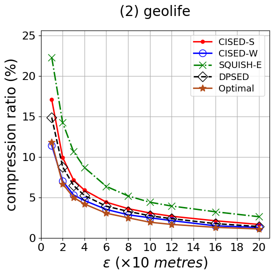
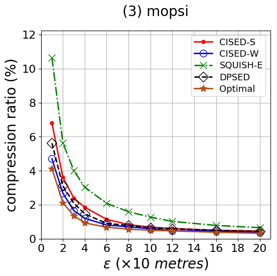
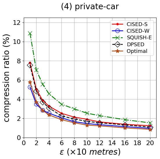
Figure 14: Evaluation of compression ratios: fixed with $m=16$ and varying error bound $\epsilon$ (on small datasets).

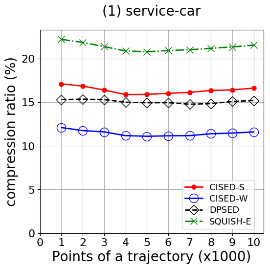
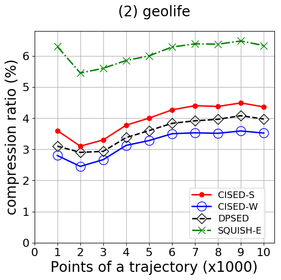
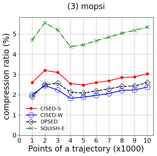
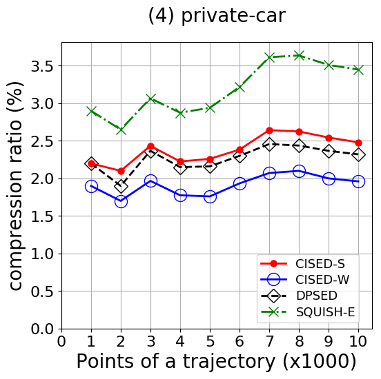
Figure 15: Evaluation of compression ratios: fixed with $m=16$ and $\epsilon=60$ meters, and varying the size of trajectories.

Exp-1.1: Impacts of parameter $m$ on compression ratios. To evaluate the impacts of the number $m$ of edges of polygons on the compression ratios of algorithms $\mathsf{CISED}$-$\mathsf{S}$ and $\mathsf{CISED}$-$\mathsf{W}$, we fixed the error bounds $\epsilon=60$ meters, and varied $m$ from $4$ to $40$. The results are reported in Figure 12.

(1) Algorithms $\mathsf{CISED}$-$\mathsf{S}$ and $\mathsf{CISED}$-$\mathsf{W}$ using $\mathsf{FastRPolyInter}$ have the same compression ratios as their counterparts using $\mathsf{CPolyInter}$ for all cases.

(2) When varying $m$, the compression ratios of algorithms $\mathsf{CISED}$-$\mathsf{S}$ and $\mathsf{CISED}$-$\mathsf{W}$ decrease with the increase of $m$ on all datasets.

(3) When varying $m$, the compression ratios of algorithms $\mathsf{CISED}$-$\mathsf{S}$ and $\mathsf{CISED}$-$\mathsf{W}$ decrease (a) fast when $m<12$, (b) slowly when $m\in[12,20]$, and (c) very slowly when $m>20$. Hence, the region of $[12,20]$ is the good candidate region for $m$ in terms of compression ratios. Here the compression ratio of $m$=$12$ is only on average $100.95\%$ of $m$=$20$.

Exp-1.2: Impacts of the error bound $\epsilon$ on compression ratios (VS. algorithms $\mathsf{DPSED}$ and $\mathsf{SQUISH}$-$\mathsf{E}$). To evaluate the impacts of error bound $\epsilon$ on compression ratios, we fixed $m$=$16$, the middle of $[12,20]$, and varied $\epsilon$ from $10$ meters to $200$ meters on the entire four datasets, respectively. The results are reported in Figure 13 .

(1) When increasing $\epsilon$, the compression ratios of all these algorithms decrease on all datasets.

(2) Dataset $\mathsf{PrivateCar}$ has the lowest compression ratios, compared with datasets $\mathsf{Mopsi}$, $\mathsf{ServiceCar}$ and $\mathsf{GeoLife}$, due to its highest sampling rate, $\mathsf{ServiceCar}$ has the highest compression ratios due to its lowest sampling rate, and $\mathsf{GeoLife}$ and $\mathsf{Mopsi}$ have the compression ratios in the middle accordingly.

(3) Algorithm $\mathsf{CISED}$-$\mathsf{S}$ is better than $\mathsf{SQUISH}$-$\mathsf{E}$and comparable with $\mathsf{DPSED}$ on all datasets and for all $\epsilon$. The compression ratios of $\mathsf{CISED}$-$\mathsf{S}$ are on average ($79.3\%$, $71.9\%$, $67.3\%$, $72.7\%$) and ($109.2\%$, $108.0\%$, $111.7\%$, $109.1\%$) of $\mathsf{SQUISH}$-$\mathsf{E}$ and $\mathsf{DPSED}$ on datasets ($\mathsf{ServiceCar}$, $\mathsf{GeoLife}$, $\mathsf{Mopsi}$, $\mathsf{PrivateCar}$), respectively. For example, when $\epsilon$ = $40$ meters, the compression ratios of algorithms $\mathsf{SQUISH}$-$\mathsf{E}$, $\mathsf{CISED}$-$\mathsf{S}$ and $\mathsf{DPSED}$ are ($20.0\%$, $8.0\%$, $5.7\%$, $4.9\%$), ($16.1\%$, $5.8\%$, $3.9\%$, $3.6\%$) and ($14.8\%$, $5.4\%$, $3.4\%$, $3.4\%$) on datasets ($\mathsf{ServiceCar}$, $\mathsf{GeoLife}$, $\mathsf{Mopsi}$, $\mathsf{PrivateCar}$), respectively.

(4) Algorithm $\mathsf{CISED}$-$\mathsf{W}$ has better compression ratios than $\mathsf{DP}$, $\mathsf{SQUISH}$-$\mathsf{E}$ and $\mathsf{CISED}$-$\mathsf{S}$ on all datasets and for all $\epsilon$. The compression ratios of $\mathsf{CISED}$-$\mathsf{W}$ are on average ($57.7\%$, $53.8\%$, $50.0\%$, $54.6\%$), ($79.5\%$, $81.0\%$, $83.0\%$, $82.0\%$) and ($72.9\%$, $75.0\%$, $74.3\%$, $75.1\%$) of algorithms $\mathsf{SQUISH}$-$\mathsf{E}$, $\mathsf{DPSED}$ and $\mathsf{CISED}$-$\mathsf{S}$ on datasets ($\mathsf{ServiceCar}$, $\mathsf{GeoLife}$, $\mathsf{Mopsi}$, $\mathsf{PrivateCar}$), respectively. For example, when $\epsilon$ = $40$ meters, the compression ratios of algorithm $\mathsf{CISED}$-$\mathsf{W}$ are ($11.5\%$, $4.3\%$, $2.8\%$, $2.7\%$) on datasets ($\mathsf{ServiceCar}$, $\mathsf{GeoLife}$, $\mathsf{Mopsi}$, $\mathsf{PrivateCar}$), respectively.

Exp-1.3: Impacts of the error bound $\epsilon$ on compression ratios (VS. the optimal algorithm). To evaluate the impacts of error bound $\epsilon$ on compression ratios, we once again fixed $m$=$16$, the middle of $[12,20]$, and varied $\epsilon$ from $10$ to $200$ meters on the first $1K$ points of each trajectory of the selected small datasets, respectively. The results are reported in Figure 14 .

(1) Algorithm $\mathsf{CISED}$-$\mathsf{S}$ is poorer than the optimal algorithm on all datasets and for all $\epsilon$. More specifically, the compression ratios of $\mathsf{CISED}$-$\mathsf{S}$ are on average ($134.6\%$, $150.7\%$, $155.5\%$, $138.5\%$) of the optimal algorithm on datasets ($\mathsf{ServiceCar}$, $\mathsf{GeoLife}$, $\mathsf{Mopsi}$, $\mathsf{PrivateCar}$), respectively. For example, when $\epsilon$ = $40$ meters, the compression ratios of $\mathsf{CISED}$-$\mathsf{S}$ and the optimal algorithm are ($22.0\%$, $5.9\%$, $1.9\%$, $3.3\%$) and ($16.4\%$, $4.2\%$, $0.9\%$, $2.4\%$) on datasets ($\mathsf{ServiceCar}$, $\mathsf{GeoLife}$, $\mathsf{Mopsi}$, $\mathsf{PrivateCar}$), respectively.

(2) Algorithm $\mathsf{CISED}$-$\mathsf{W}$ is comparable with the optimal algorithm on all datasets and for all $\epsilon$. The compression ratios of $\mathsf{CISED}$-$\mathsf{W}$ are on average ($94.8\%$, $115.5\%$, $119.7\%$, $107.5\%$) of the optimal algorithm on datasets ($\mathsf{ServiceCar}$, $\mathsf{GeoLife}$, $\mathsf{Mopsi}$, $\mathsf{PrivateCar}$), respectively. For example, when $\epsilon$ = $40$ meters, the compression ratios of algorithm $\mathsf{CISED}$-$\mathsf{W}$ are ($14.6\%$, $4.6\%$, $1.2\%$, $2.5\%$) on datasets ($\mathsf{ServiceCar}$, $\mathsf{GeoLife}$, $\mathsf{Mopsi}$, $\mathsf{PrivateCar}$), respectively.

Exp-1.4: Impacts of trajectory sizes on compression ratios. To evaluate the impacts of trajectory size, i.e., the number of data points in a trajectory, on compression ratios, we chose the same $10$ trajectories from datasets $\mathsf{ServiceCar}$, $\mathsf{GeoLife}$, $\mathsf{Mopsi}$ and $\mathsf{PrivateCar}$, respectively, fixed $m$=$16$ and $\epsilon$=$60$ meters, and varied the size $\dddot{\mathcal{|T|}}$ of trajectories from $1K$ points to $10K$ points. The results are reported in Figure 15.

(1) The compression ratios of these algorithms from the best to the worst are $\mathsf{CISED}$-$\mathsf{W}$, $\mathsf{DPSED}$, $\mathsf{CISED}$-$\mathsf{S}$ and $\mathsf{SQUISH}$-$\mathsf{E}$, on all datasets and for all sizes of trajectories.

(2) The size of input trajectories has few impacts on the compression ratios of $\mathsf{LS}$ algorithms on all datasets.

5.2.2 Evaluation of Average Errors

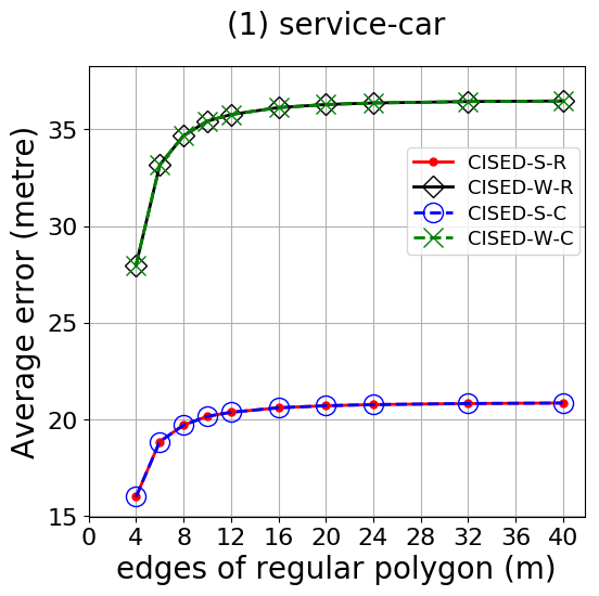
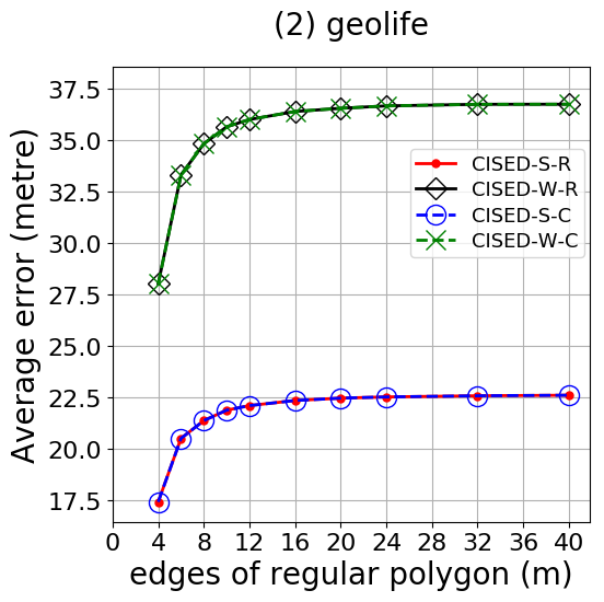
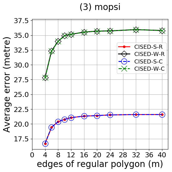
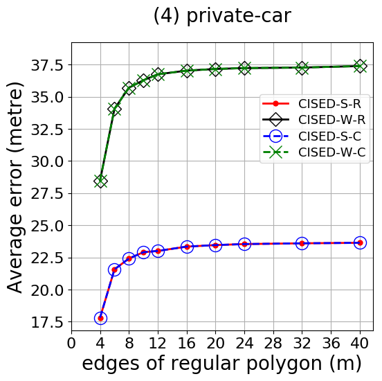
Figure 16: Evaluation of average errors: fixed error bound with $\epsilon=60$ meters and varying $m$.

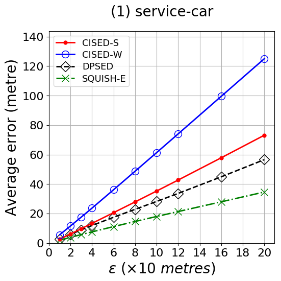
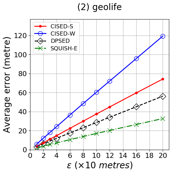
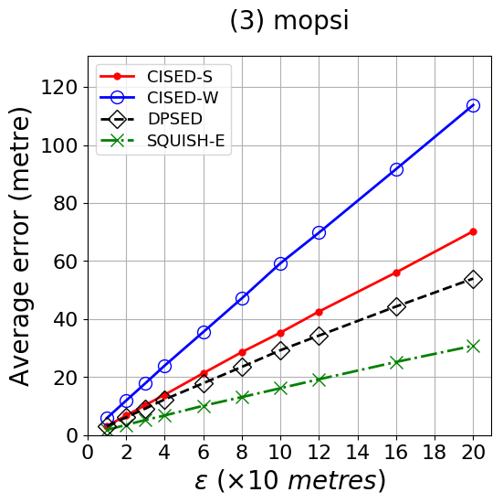
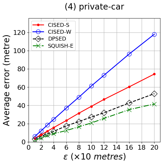
Figure 17: Evaluation of average errors: fixed with $m=16$ and varying error bound $\epsilon$.

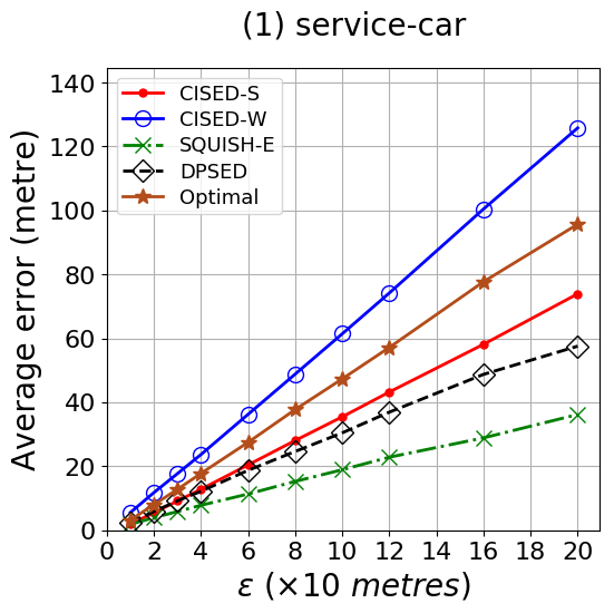
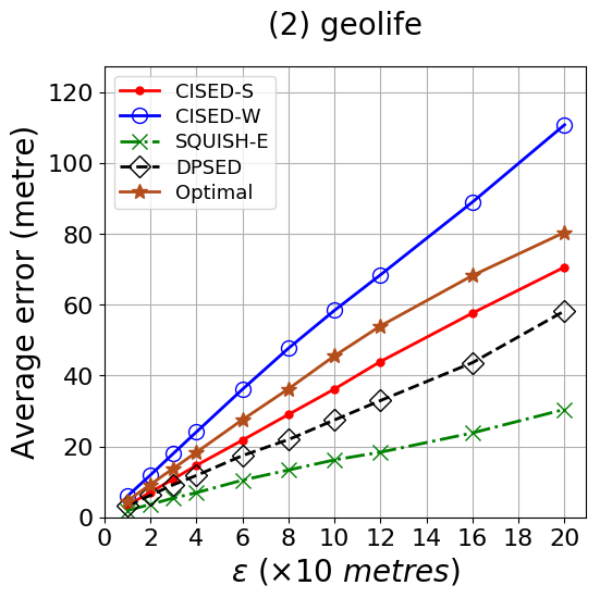
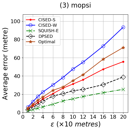
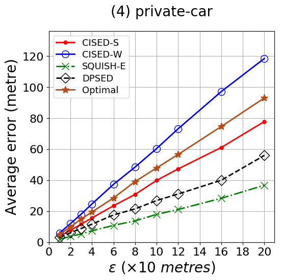
Figure 18: Evaluation of average errors: fixed with $m=16$ and varying error bound $\epsilon$ (on small datasets).

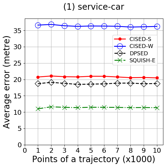
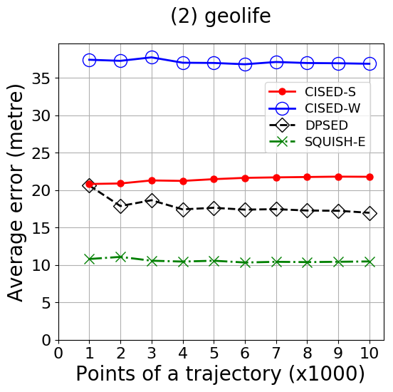
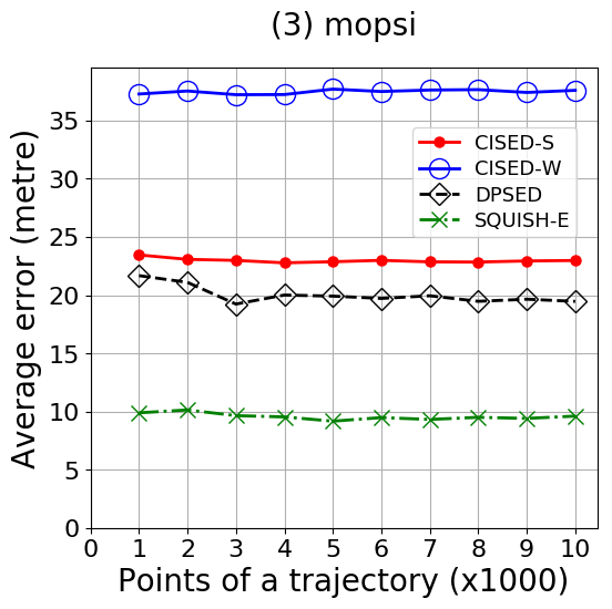
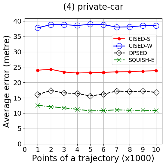
Figure 19: Evaluation of average errors: fixed with $m=16$ and $\epsilon=60$ meters, and varying the size of trajectories.

In the second set of tests, we first evaluate the impacts of parameter $m$ on the average errors of algorithms $\mathsf{CISED}$-$\mathsf{S}$ and $\mathsf{CISED}$-$\mathsf{W}$, then compare the average errors of our algorithms $\mathsf{CISED}$-$\mathsf{S}$ and $\mathsf{CISED}$-$\mathsf{W}$ with $\mathsf{DPSED}$, $\mathsf{SQUISH}$-$\mathsf{E}$ and the optimal algorithm.

Given a set of trajectories $\{\dddot{\mathcal{T}_{1}},\ldots,\dddot{\mathcal{T}}_{M}\}$ and their piecewise line representations $\{\overline{\mathcal{T}_{1}},\ldots,\overline{\mathcal{T}}_{M}\}$, and point $P_{j,i}$ denoting a point in trajectory $\dddot{\mathcal{T}}_{j}$ contained in a line segment $\mathcal{L}_{l,i}\in\overline{\mathcal{T}_{l}}$ ($l\in[1,M]$), then the average error is $\sum_{j=1}^{M}\sum_{i=0}^{M}d(P_{j,i},\mathcal{L}_{l,i})/\sum_{j=1}^{M}{|\dddot{\mathcal{T}}_{j}|}$.

Exp-2.1: Impacts of parameter $m$ on average errors. To evaluate the impacts of parameter $m$ on average errors of algorithms $\mathsf{CISED}$-$\mathsf{S}$ and $\mathsf{CISED}$-$\mathsf{W}$, we fixed the error bounds $\epsilon=60$ meters, and varied $m$ from $4$ to $40$. The results are reported in Figure 16.

(1) Algorithms $\mathsf{CISED}$-$\mathsf{S}$ and $\mathsf{CISED}$-$\mathsf{W}$ using $\mathsf{FastRPolyInter}$ have the same average errors as their counterparts using $\mathsf{CPolyInter}$, respectively, on all datasets and for all $m$.

(2) When varying $m$, the average errors of algorithms $\mathsf{CISED}$-$\mathsf{S}$ and $\mathsf{CISED}$-$\mathsf{W}$ increase with the increase of $m$ on all datasets.

(3) When varying $m$, similar to compression ratios, the average errors of algorithms $\mathsf{CISED}$-$\mathsf{S}$ and $\mathsf{CISED}$-$\mathsf{W}$ increase (a) fast when $m<12$, (b) slowly when $m\in[12,20]$, and (c) very slowly when $m>20$. The range of $[12,20]$ is also the good candidate region for $m$ in terms of errors. Here the average error of $m=12$ is only on average $98.49\%$ of $m=20$.

Exp-2.2: Impacts of the error bound $\epsilon$ on average errors (VS. algorithms $\mathsf{DPSED}$ and $\mathsf{SQUISH}$-$\mathsf{E}$). To evaluate the average errors of these algorithms, we fixed $m$=$16$, and varied $\epsilon$ from $10$ meters to $200$ meters on the entire datasets $\mathsf{ServiceCar}$, $\mathsf{GeoLife}$, $\mathsf{Mopsi}$ and $\mathsf{PrivateCar}$, respectively. The results are reported in Figure 17.

(1) Average errors increase with the increase of $\epsilon$.

(2) The average errors of these algorithms from the largest to the smallest are $\mathsf{CISED}$-$\mathsf{W}$, $\mathsf{CISED}$-$\mathsf{S}$, $\mathsf{DPSED}$ and $\mathsf{SQUISH}$-$\mathsf{E}$, on all datasets and for all $\epsilon$. The average errors of algorithms $\mathsf{CISED}$-$\mathsf{S}$ and $\mathsf{CISED}$-$\mathsf{W}$ are on average ($119.3\%$, $127.7\%$, $119.9\%$, $138.0\%$) and ($210.1\%$, $207.5\%$, $200.9\%$, $217.5\%$) of $\mathsf{DPSED}$ and ($188.2\%$, $215.2\%$, $212.8\%$, $180.3\%$) and ($331.1\%$, $349.7\%$, $356.7\%$, $284.2\%$) of $\mathsf{SQUISH}$-$\mathsf{E}$ on datasets ($\mathsf{ServiceCar}$, $\mathsf{GeoLife}$, $\mathsf{Mopsi}$, $\mathsf{PrivateCar}$), respectively.

(3) When the error bound of algorithm $\mathsf{CISED}$-$\mathsf{W}$ is set as the half of $\mathsf{CISED}$-$\mathsf{S}$, the average errors of $\mathsf{CISED}$-$\mathsf{W}$ are on average ($93.8\%$, $86.0\%$, $81.4\%$, $79.4\%$) of $\mathsf{CISED}$-$\mathsf{S}$ on datasets ($\mathsf{ServiceCar}$, $\mathsf{GeoLife}$,$\mathsf{Mopsi}$, $\mathsf{PrivateCar}$), respectively, meaning that the large average errors of algorithm $\mathsf{CISED}$-$\mathsf{W}$ are caused by its cone w.r.t. $\epsilon$ compared with the narrow cone w.r.t. $\epsilon/2$ of $\mathsf{CISED}$-$\mathsf{S}$.

Exp-2.3: Impacts of the error bound $\epsilon$ on average errors (VS. the optimal algorithm). To evaluate the average errors of these algorithms, we once again fixed $m$=$16$, and varied $\epsilon$ from $10$ meters to $200$ meters on the first $1K$ points of each trajectory of the selected small datasets, respectively. The results are reported in Figure 18.

The average errors of these algorithms from the largest to the smallest are $\mathsf{CISED}$-$\mathsf{W}$, the optimal algorithm and $\mathsf{CISED}$-$\mathsf{S}$, on all datasets and for all $\epsilon$. The average errors of $\mathsf{CISED}$-$\mathsf{S}$ and $\mathsf{CISED}$-$\mathsf{W}$ are on average ($73.6\%$, $80.7\%$, $85.1\%$, $81.0\%$) and ($133.3\%$, $130.7\%$, $131.0\%$, $126.3\%$) of the optimal algorithm on datasets ($\mathsf{ServiceCar}$, $\mathsf{GeoLife}$, $\mathsf{Mopsi}$, $\mathsf{PrivateCar}$), respectively.

Exp-2.4: Impacts of trajectory sizes on average errors. To evaluate the impacts of trajectory sizes on average errors, we chose the same $10$ trajectories from datasets $\mathsf{ServiceCar}$, $\mathsf{GeoLife}$, $\mathsf{Mopsi}$ and $\mathsf{PrivateCar}$, respectively. We fixed $m$=$16$ and $\epsilon=60$ meters, and varied the size $\dddot{\mathcal{|T|}}$ of trajectories from $1K$ points to $10K$ points. The results are reported in Figure 19.

(1) The average errors of these algorithms from the smallest to the largest are $\mathsf{SQUISH}$-$\mathsf{E}$, $\mathsf{DPSED}$, $\mathsf{CISED}$-$\mathsf{S}$ and $\mathsf{CISED}$-$\mathsf{W}$, on all datasets and for all trajectory sizes.

(2) The size of input trajectories has few impacts on the average errors of $\mathsf{LS}$ algorithms on all datasets.

5.2.3 Evaluation of Efficiency

In the last set of tests, we evaluate the impacts of parameter $m$ on the efficiency of algorithms $\mathsf{CISED}$-$\mathsf{S}$ and $\mathsf{CISED}$-$\mathsf{W}$, and compare the efficiency of our approaches $\mathsf{CISED}$-$\mathsf{S}$ and $\mathsf{CISED}$-$\mathsf{W}$ with the optimal algorithm and algorithms $\mathsf{DPSED}$ and $\mathsf{SQUISH}$-$\mathsf{E}$.

Exp-3.1: Impacts of algorithm $\mathsf{FastRPolyInter}$ and parameter $m$ on efficiency. To evaluate the impacts of $\mathsf{FastRPolyInter}$ and parameter $m$ on algorithm $\mathsf{CISED}$-$\mathsf{S}$ and $\mathsf{CISED}$-$\mathsf{W}$, we equipped $\mathsf{CISED}$-$\mathsf{S}$ and $\mathsf{CISED}$-$\mathsf{W}$ with $\mathsf{FastRPolyInter}$ and $\mathsf{CPolyInter}$, respectively, fixed $\epsilon=60$ meters, and varied $m$ from $4$ to $40$. The results are reported in Figures 20 and 21.

(1) The algorithms $\mathsf{CISED}$-$\mathsf{S}$ and $\mathsf{CISED}$-$\mathsf{W}$ spend the most time in the executing of polygon intersections. For all $m$, the execution time of algorithms $\mathsf{CPolyInter}$ and $\mathsf{FastRPolyInter}$ is on average ($93.5\%$, $96.0\%$, $94.5\%$, $92.0\%$) and ($90.5\%$, $92.5\%$, $91.0\%$, $90.5\%$) of the entire compression time on datasets ($\mathsf{ServiceCar}$, $\mathsf{GeoLife}$, $\mathsf{Mopsi}$, $\mathsf{PrivateCar}$), respectively.

(2) $\mathsf{FastRPolyInter}$ runs faster than $\mathsf{CPolyInter}$ on all datasets and for all $m$. The execution time of algorithms $\mathsf{CISED}$-$\mathsf{S}$-$\mathsf{FastRPolyInter}$ and $\mathsf{CISED}$-$\mathsf{W}$-$\mathsf{FastRPolyInter}$ is one average $83.74\%$ their counterparts with $\mathsf{CPolyInter}$.

(3) When varying $m$, the execution time of algorithms $\mathsf{CISED}$-$\mathsf{S}$-$\mathsf{FastRPolyInter}$, $\mathsf{CISED}$-$\mathsf{S}$-$\mathsf{CPolyInter}$, $\mathsf{CISED}$-$\mathsf{W}$-$\mathsf{FastRPolyInter}$ and $\mathsf{CISED}$-$\mathsf{W}$-$\mathsf{CPolyInter}$ increases approximately linearly with the increase of $m$ on all the datasets.

(4) The running time of $m=12$ is on average $69.92\%$ of $m=20$ for $\mathsf{CISED}$-$\mathsf{S}$ and $\mathsf{CISED}$-$\mathsf{W}$ on all datasets.

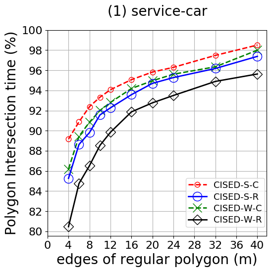
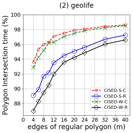
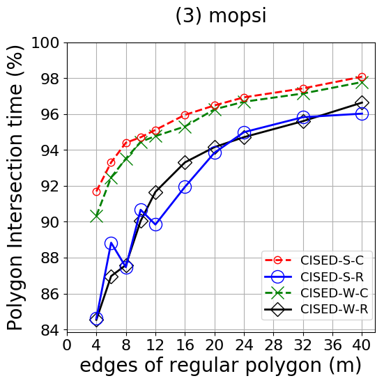
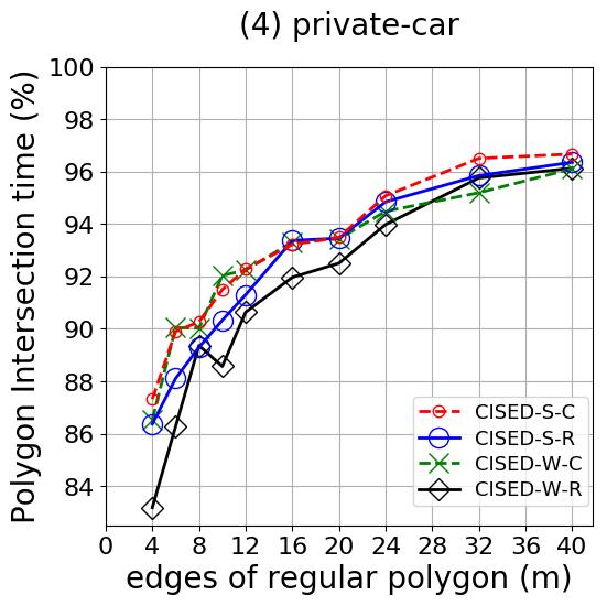
Figure 20: Evaluation of running time of polygon intersection algorithms: fixed error bound with $\epsilon=60$ meters, and varying $m$. Here “R” denotes our fast regular polygon intersection algorithm $\mathsf{FastRPolyInter}$, and “C” denotes $\mathsf{CPolyInter}$, respectively.

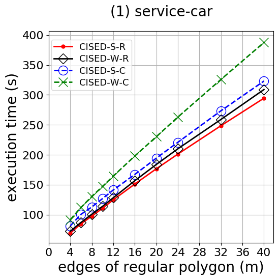
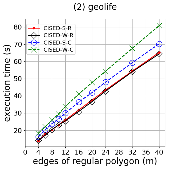
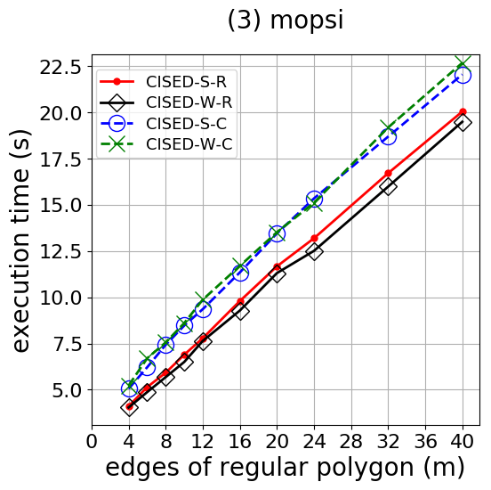
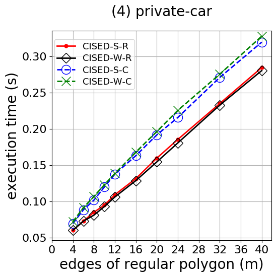
Figure 21: Evaluation of running time: fixed error bound with $\epsilon=60$ meters, and varying $m$.

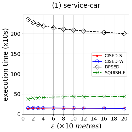
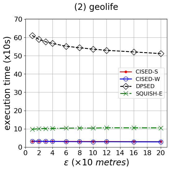
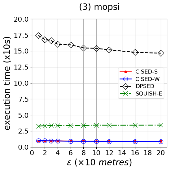
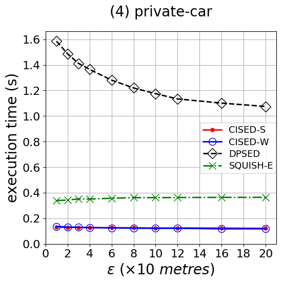
Figure 22: Evaluation of running time: fixed with $m=16$ and varying error bounds $\epsilon$.

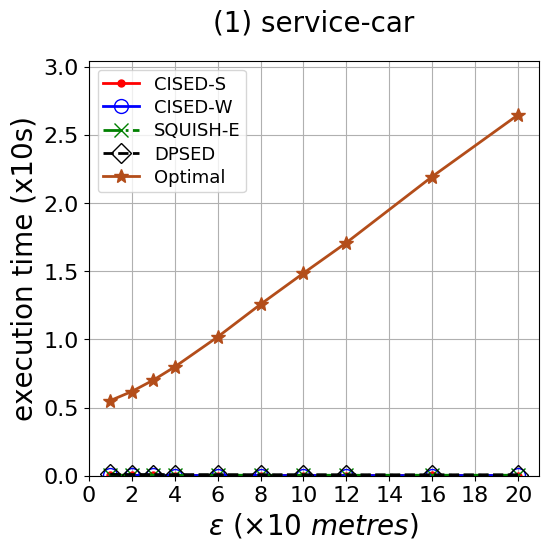
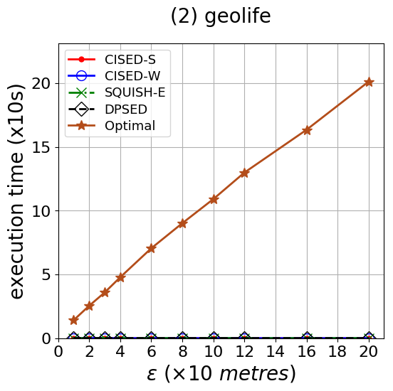
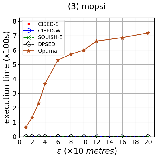
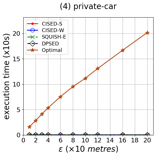
Figure 23: Evaluation of running time: fixed with $m=16$ and varying error bounds $\epsilon$ (on small datasets).

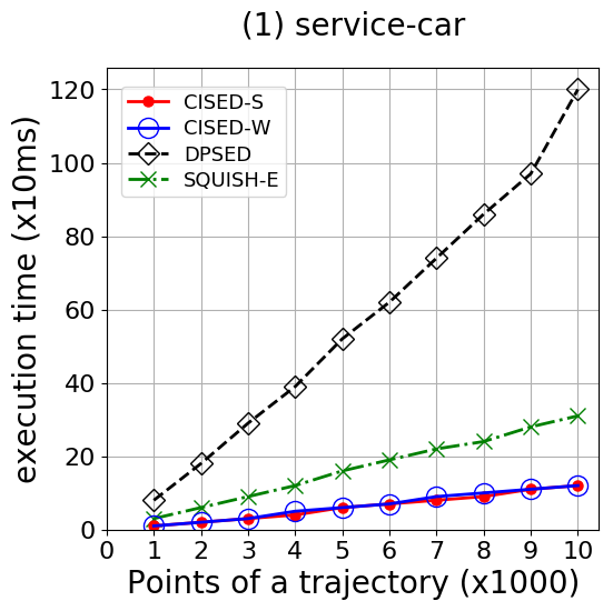
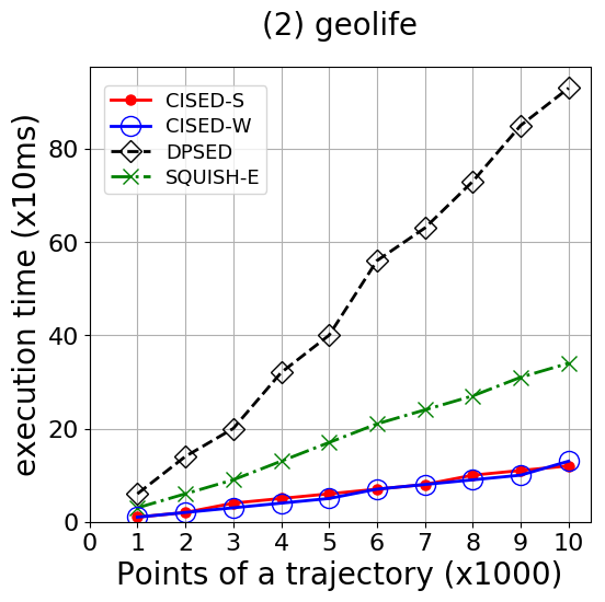
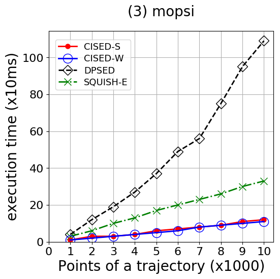
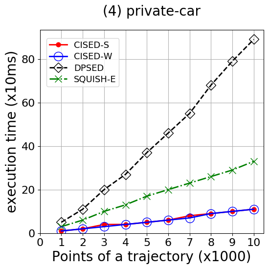
Figure 24: Evaluation of running time: fixed with $m=16$ and $\epsilon=60$ meters, and varying the size of trajectories.

Exp-3.2: Impacts of the error bound $\epsilon$ on efficiency (VS. algorithms $\mathsf{DPSED}$ and $\mathsf{SQUISH}$-$\mathsf{E}$). To evaluate the impacts of $\epsilon$ on efficiency, we fixed $m$ = $16$, and varied $\epsilon$ from $10$ meters to $200$ meters on the entire datasets ($\mathsf{ServiceCar}$, $\mathsf{GeoLife}$, $\mathsf{Mopsi}$, $\mathsf{PrivateCar}$), respectively. The results are reported in Figure 22.

(1) All algorithms are not very sensitive to $\epsilon$ on any datasets, and algorithm $\mathsf{DPSED}$ is more sensitive to $\epsilon$ than the other three algorithms. The running time of $\mathsf{DPSED}$ decreases a little bit with the increase of $\epsilon$, as the increment of $\epsilon$ decreases the number of partitions of the input trajectory.

(2) Algorithms $\mathsf{CISED}$-$\mathsf{S}$ and $\mathsf{CISED}$-$\mathsf{W}$ are obviously faster than $\mathsf{DPSED}$ and $\mathsf{SQUISH}$-$\mathsf{E}$ for all cases. They are on average ($14.21$, $18.19$, $17.06$, $9.98$) times faster than $\mathsf{DPSED}$, and ($2.84$, $3.45$, $3.69$, $2.86$) times faster than $\mathsf{SQUISH}$-$\mathsf{E}$ on datasets ($\mathsf{ServiceCar}$, $\mathsf{GeoLife}$, $\mathsf{Mopsi}$, $\mathsf{PrivateCar}$), respectively.

Exp-3.3: Impacts of the error bound $\epsilon$ on efficiency (VS. the optimal algorithm). To evaluate the impacts of $\epsilon$ on efficiency, we once again fixed $m$ = $16$, and varied $\epsilon$ from $10$ meters to $200$ meters on the first $1K$ points of each trajectory of the selected small datasets, respectively. The results are reported in Figure 23.

(1) Algorithms $\mathsf{CISED}$-$\mathsf{S}$ and $\mathsf{CISED}$-$\mathsf{W}$ are obviously faster than the optimal algorithm for all cases. They are on average ($925.25$, $7888.26$, $40041.59$, $8528.76$) times faster than the optimal algorithm on datasets ($\mathsf{ServiceCar}$, $\mathsf{GeoLife}$, $\mathsf{Mopsi}$, $\mathsf{PrivateCar}$), respectively.

Exp-3.4: Impacts of trajectory sizes on efficiency. To evaluate the impacts of trajectory sizes on execution time, we chose the same $10$ trajectories, from datasets ($\mathsf{ServiceCar}$, $\mathsf{GeoLife}$, $\mathsf{Mopsi}$, $\mathsf{PrivateCar}$), respectively, fixed $m$ = $16$ and $\epsilon=60$ meters, and varied the size $\dddot{\mathcal{|T|}}$ of trajectories from $1K$ points to $10K$ points. The results are reported in Figure 24.

(1) Algorithms $\mathsf{CISED}$-$\mathsf{S}$ and $\mathsf{CISED}$-$\mathsf{W}$ are both the fastest $\mathsf{LS}$ algorithms using $\mathsf{SED}$, and are ($8.00$–$10.00$, $5.83$–$8.11$, $4.00$–$9.50$, $5.00$–$8.09$) times faster than $\mathsf{DPSED}$, and ($2.53$–$3.00$, $2.62$–$3.12$, $2.50$–$3.33$, $2.89$–$3.40$) times faster than $\mathsf{SQUISH}$-$\mathsf{E}$ on the selected $1K$ to $10K$ points datasets ($\mathsf{ServiceCar}$, $\mathsf{GeoLife}$, $\mathsf{Mopsi}$, $\mathsf{PrivateCar}$), respectively.

(2) Algorithms $\mathsf{CISED}$-$\mathsf{S}$ and $\mathsf{CISED}$-$\mathsf{W}$ scale well with the increase of the size of trajectories on all datasets, and both have a linear running time, while algorithm $\mathsf{DPSED}$ does not. This is consistent with their time complexity analyses.

(3) The efficiency advantage of algorithms $\mathsf{CISED}$-$\mathsf{S}$ and $\mathsf{CISED}$-$\mathsf{W}$ increases with the increase of trajectory sizes compared with $\mathsf{DPSED}$ and $\mathsf{SQUISH}$-$\mathsf{E}$.

5.2.4 Summary

From these tests we find the following.

(1) Polygon intersection Algorithms. Algorithm $\mathsf{FastRPolyInter}$ runs faster than $\mathsf{CPolyInter}$, and is as effective as $\mathsf{CPolyInter}$.

(2) Parameter $m$. The compression ratio decreases with the increase of $m$, and the running time increases nearly linearly with the increase of $m$. In practice, the range of $[12,20]$ is a good candidate region for $m$.

(3) Compression ratios. The optimal $\mathsf{LS}$ algorithm has the best compression ratios among all strong simplification algorithms. Algorithm $\mathsf{CISED}$-$\mathsf{S}$ is comparable with $\mathsf{DPSED}$ and algorithm $\mathsf{CISED}$-$\mathsf{W}$ is comparable with the optimal $\mathsf{LS}$ algorithm. They are all better than $\mathsf{SQUISH}$-$\mathsf{E}$. The compression ratios of algorithm $\mathsf{CISED}$-$\mathsf{S}$, the optimal algorithm and algorithm $\mathsf{CISED}$-$\mathsf{W}$ are on average ($79.3\%$, $71.9\%$, $67.3\%$, $72.7\%$), ($58.1\%$, $45.1\%$, $39.2\%$, $52.8\%$) and ($57.7\%$, $53.8\%$, $50.0\%$, $54.6\%$) of $\mathsf{SQUISH}$-$\mathsf{E}$ and ($109.2\%$, $108.0\%$, $111.7\%$, $109.1\%$), ($81.3\%$, $75.5\%$, $72.5\%$, $78.1\%$) and ($79.5\%$, $81.0\%$, $83.0\%$, $82.0\%$) of $\mathsf{DPSED}$ on datasets ($\mathsf{ServiceCar}$, $\mathsf{GeoLife}$, $\mathsf{Mopsi}$, $\mathsf{PrivateCar}$), respectively.

(4) Average errors. The average errors of these algorithms from the smallest to the largest are $\mathsf{SQUISH}$-$\mathsf{E}$, $\mathsf{DPSED}$, $\mathsf{CISED}$-$\mathsf{S}$, the optimal $\mathsf{LS}$ algorithm and $\mathsf{CISED}$-$\mathsf{W}$. Algorithm $\mathsf{CISED}$-$\mathsf{W}$ has obvious higher average errors than $\mathsf{CISED}$-$\mathsf{S}$ as the former essentially forms spatio-temporal cones with a radius of $\epsilon$.

(5) Running time. Algorithms $\mathsf{CISED}$-$\mathsf{S}$ and $\mathsf{CISED}$-$\mathsf{W}$ are the fastest. They are on average ($14.21$, $18.19$, $17.06$, $9.98$), ($2.84$, $3.45$, $3.69$, $2.86$) and ($925.25$, $7888.26$, $40041.59$, $8528.76$) times faster than $\mathsf{DPSED}$, $\mathsf{SQUISH}$-$\mathsf{E}$ and the optimal $\mathsf{LS}$ algorithm on datasets ($\mathsf{ServiceCar}$, $\mathsf{GeoLife}$, $\mathsf{Mopsi}$, $\mathsf{PrivateCar}$), respectively. The efficiency advantage of algorithms $\mathsf{CISED}$-$\mathsf{S}$ and $\mathsf{CISED}$-$\mathsf{W}$ also increases with the increase of the trajectory size.

6 Related Work

Trajectory compression algorithms are normally classified into two categories, namely lossless compression and lossy compressionMuckell:Compression . (1) Lossless compression methods enable exact reconstruction of the original data from the compressed data without information loss. (2) In contrast, lossy compression methods allow errors or derivations, compared with the original trajectories. These techniques typically identify important data points, and remove statistical redundant data points from a trajectory, or replace original data points in a trajectory with other places of interests, such as roads and shops. They focus on good compression ratios with acceptable errors. In this work, we focus on lossy compression of trajectory data, and we next introduce the related work on lossy trajectory compression from two aspects: line simplification based methods and semantics based methods.

6.1 Line simplification based methods

The idea of piece-wise line simplification comes from computational geometry. Its target is to approximate a given finer piece-wise linear curve by another coarser piece-wise linear curve, which is typically a subset of the former, such that the maximum distance of the former to the later is bounded by a user specified bound $\epsilon$. Initially, line simplification ($\mathsf{LS}$) algorithms use perpendicular Euclidean distances ($\mathsf{PED}$) as the distance metric. Then a new distance metric, the synchronous Euclidean distances ($\mathsf{SED}$), was developed after the $\mathsf{LS}$ algorithms were introduced to compress trajectories. $\mathsf{SED}$ was first introduced in the name of time-ratio distance in Meratnia:Spatiotemporal , and formally presented in Potamias:Sampling as the synchronous Euclidean distance. $\mathsf{PED}$ and $\mathsf{SED}$ are two common metrics adopted in trajectory simplification. The former usually brings better compression ratios while the later reserves temporal information in the result trajectories.

Line simplification algorithms can be classified into two aspects: optimal and sub-optimal methods.

6.1.1 Optimal Algorithms

For the “min-#” problem that finds out the minimal number of points or segments to represent the original polygonal lines w.r.t. an error bound $\epsilon$, Imai and Iri Imai:Optimal first formulated it as a graph problem, and showed that it could be solved in $O(n^{3})$ time, where $n$ is the number of the original points. Toussaint of Toussaint:Optimal and Melkman and O’Rourke of Melkman:Optimal improved the time complexity to $O(n^{2}\log n)$ by using either convex hull or sector intersection methods. The authors of Chan:Optimal further proved that the optimal algorithm using $\mathsf{PED}$ could be implemented in $O(n^{2})$ time by using the sector intersection mechanism. Because the sector intersection and the convex hull mechanisms can not work with $\mathsf{SED}$, hence, currently the time complexity of the optimal algorithm using $\mathsf{SED}$ remains $O(n^{3})$. It is time-consuming and impractical for large trajectory data Heckbert:Survey .

6.1.2 Sub-optimal Algorithms

Many studies have been targeting at finding the sub-optimal results. In particular, the state-of-the-art of sub-optimal $\mathsf{LS}$ approaches fall into three categories, i.e., batch, online and one-pass algorithms. We next introduce these $\mathsf{LS}$ based trajectory compression algorithms from the aspect of the three categories.

Batch algorithms. The batch algorithms adopt a global distance checking policy that requires all trajectory points are loaded before compressing starts. These batch algorithms can be either top-down or bottom-up.

Top-down algorithms, e.g., Ramer Ramer:Split and Douglas-Peucker Douglas:Peucker , recursively divide a trajectory into sub-trajectories until the stopping condition is met. Bottom-up algorithms, e.g., Theo Pavlidis’ algorithm Pavlidis:Segment , is the natural complement of the top-down ones, which recursively merge adjacent sub-trajectories with the smallest distance, initially $n/2$ sub-trajectories for a trajectory with $n$ points, until the stopping condition is met. The distances of newly generated line segments are recalculated during the process. These batch algorithms originally only support $\mathsf{PED}$, but are easy to be extended to support $\mathsf{SED}$ Meratnia:Spatiotemporal . The batch nature and high time complexities make batch algorithms impractical for online and resource-constrained scenarios Lin:Operb .

Online algorithms. The online algorithms adopt a constrained global distance checking policy that restricts the checking within a sliding or opening window. Constrained global checking algorithms do not need to have the entire trajectory ready before they start compressing, and are more appropriate than batch algorithm for compressing trajectories for online scenarios.

Several $\mathsf{LS}$ algorithms have been developed, e.g., by combining $\mathsf{DP}$ or $\mathsf{Theo\leavevmode\nobreak\ Pavlidis^{\prime}}$ with sliding or opening windows for online processingMeratnia:Spatiotemporal . These methods still have a high time and/or space complexity, which significantly hinders their utility in resource-constrained mobile devices Liu:BQS . $\mathsf{BQS}$ Liu:BQS ; Liu:Amnesic and $\mathsf{SQUISH}$-$\mathsf{E}$ Muckell:Compression further optimize the opening window algorithms. $\mathsf{BQS}$ Liu:BQS ; Liu:Amnesic fasts the processing by picking out at most eight special points from an open window based on a convex hull, which, however, hardly supports $\mathsf{SED}$. The $\mathsf{SQUISH}$-$\mathsf{E}$ Muckell:Compression algorithm is an combination of opening window and bottom-up online algorithm. It uses a doubly linked list $Q$ to achieve a better efficiency. Although $\mathsf{SQUISH}$-$\mathsf{E}$ supports $\mathsf{SED}$, it is not one-pass, and has a relatively poor compression ratio.

One-pass algorithms. The one-pass algorithms adopt a local distance checking policy. They do not need a window to buffer the previously read points as they process each point in a trajectory once and only once. Obviously, the one-pass algorithms run in linear time and constant space.

The $n$–${th}$ point routine and the routine of random-selection of points Shi:Survey are two naive one-pass algorithms. In these routines, for every fixed number of consecutive points along the line, the $n$–${th}$ point and one random point among them are retained, respectively. They are fast, but are obviously not error bounded. In Reumann-Witkam routineReumann:Strip , it builds a strip paralleling to the line connecting the first two points, then the points within this strip compose one section of the line. The Reumann-Witkam routine also runs fast, but has limited compression ratios. The sector intersection ($\mathsf{SI}$) algorithm Williams:Longest ; Sklansky:Cone was developed for graphic and pattern recognition in the late 1970s, for the approximation of arbitrary planar curves by linear segments or finding a polygonal approximation of a set of input data points in a 2D Cartesian coordinate system. Dunham:Cone optimized algorithm $\mathsf{SI}$ by considering the distance between a potential end point and the initial point of a line segment, and the $\mathsf{Sleeve}$ algorithm Zhao:Sleeve in the cartographic discipline essentially applies the same idea as the $\mathsf{SI}$ algorithm. Moreover, fast $\mathsf{BQS}$ Liu:BQS ($\mathsf{FBQS}$ in short), the simplified version of $\mathsf{BQS}$, has a linear time complexity. The authors of this article also developed an One-Pass ERror Bounded ($\mathsf{OPERB}$) algorithm Lin:Operb . However, all existing one-pass algorithms use $\mathsf{PED}$ Williams:Longest ; Sklansky:Cone ; Dunham:Cone ; Zhao:Sleeve ; Liu:BQS ; Lin:Operb , while this study focuses on $\mathsf{SED}$.

6.2 Semantics based methods

The trajectories of certain moving objects such as cars and trucks are constrained by road networks. These moving objects typically travel along road networks, instead of the line segment between two points. Trajectory compression methods based on road networks Chen:Trajectory ; Popa:Spatio ; Civilis:Techniques ; Hung:Clustering ; Gotsman:Compaction ; Song:PRESS ; Han:Compress project trajectory points onto roads (also known as Map-Matching). Moreover, Gotsman:Compaction ; Song:PRESS ; Han:Compress mine and use high frequency patterns of compressed trajectories, instead of roads, to further improve compression effectiveness. Some methods Schmid:Semantic ; Richter:Semantic compress trajectories beyond the use of road networks, and further make use of other user specified domain knowledge, such as places of interests along the trajectories Richter:Semantic . There are also compression algorithms preserving the direction of the trajectory Long:Direction .

These semantics based approaches are orthogonal to line simplification based methods, and may be combined with each other to improve the effectiveness of trajectory compression.

7 Conclusions

We have proposed $\mathsf{CISED}$-$\mathsf{S}$ and $\mathsf{CISED}$-$\mathsf{W}$, two one-pass error bounded strong and weak trajectory simplification algorithms using the synchronous distance. We have also experimentally verified that algorithms $\mathsf{CISED}$-$\mathsf{S}$ and $\mathsf{CISED}$-$\mathsf{W}$ are both efficient and effective. They are three times faster than $\mathsf{SQUISH}$-$\mathsf{E}$, the most efficient existing $\mathsf{LS}$ algorithm using $\mathsf{SED}$. In terms of compression ratio, algorithm $\mathsf{CISED}$-$\mathsf{S}$ is comparable with $\mathsf{DPSED}$, the existing $\mathsf{LS}$ algorithm with the best compression ratio, and is $21.1\%$ better than $\mathsf{SQUISH}$-$\mathsf{E}$ on average; and algorithm $\mathsf{CISED}$-$\mathsf{W}$ is comparable with the optimal algorithm and is on average $19.6\%$ and $42.4\%$ better than $\mathsf{DPSED}$ and $\mathsf{SQUISH}$-$\mathsf{E}$, respectively.

References

- [1] Mopsi routes 2014. http://cs.uef.fi/mopsi/routes/dataset/. Accessed: 2017-11-29.
- [2] H. Cao, O. Wolfson, and G. Trajcevski. Spatio-temporal data reduction with deterministic error bounds. VLDBJ, 15(3):211–228, 2006.
- [3] W. Chan and F. Chin. Approximation of polygonal curves with minimum number of line segments or minimal error. International Journal of Computational Geometry Applicaitons, 6(1):378–387, 1996.
- [4] M. Chen, M. Xu, and P. Fränti. A fast multiresolution polygonal approximation algorithm for GPS trajectory simplification. IEEE Trans. Image Processing, 21(5):2770–2785, 2012.
- [5] Y. Chen, K. Jiang, Y. Zheng, C. Li, and N. Yu. Trajectory simplification method for location-based social networking services. In LBSN, pages 33–40, 2009.
- [6] A. Civilis, C. S. Jensen, and S. Pakalnis. Techniques for efficient road-network-based tracking of moving objects. TKDE, 17(5):698–712, 2005.
- [7] D. H. Douglas and T. K. Peucker. Algorithms for the reduction of the number of points required to represent a digitized line or its caricature. The Canadian Cartographer, 10(2):112–122, 1973.
- [8] J. G. Dunham. Piecewise linear approximation of plannar curves. PAMI, 8, 1986.
- [9] R. Gotsman and Y. Kanza. A dilution-matching-encoding compaction of trajectories over road networks. GeoInformatica, 2015.
- [10] Y. Han, W. Sun, and B. Zheng. Compress: A comprehensive framework of trajectory compression in road networks. TODS, 42(2):11:1–11:49, 2017.
- [11] P. S. Heckbert and M. Garland. Survey of polygonal surface simplification algorithms. In SIGGRAPH, 1997.
- [12] J. Hershberger and J. Snoeyink. Speeding up the douglas-peucker line-simplification algorithm. Technical Report, University of British Columbia, 1992.
- [13] C. C. Hung, W. Peng, and W. Lee. Clustering and aggregating clues of trajectories for mining trajectory patterns and routes. VLDBJ, 24(2):169–192, 2015.
- [14] H. Imai and M. Iri. Computational-geometric methods for polygonal approximations of a curve. Computer Vision Graphics and Image Processing, 36:31–41, 1986.
- [15] X. Lin, S. Ma, H. Zhang, T. Wo, and J. Huai. One-pass error bounded trajectory simplification. PVLDB, 10(7):841–852, 2017.
- [16] J. Liu, K. Zhao, P. Sommer, S. Shang, B. Kusy, and R. Jurdak. Bounded quadrant system: Error-bounded trajectory compression on the go. In ICDE, 2015.
- [17] J. Liu, K. Zhao, P. Sommer, S. Shang, B. Kusy, J.-G. Lee, and R. Jurdak. A novel framework for online amnesic trajectory compression in resource-constrained environments. IEEE Transactions on Knowledge and Data Engineering, 28(11):2827–2841, 2016.
- [18] C. Long, R. C.-W. Wong, and H. Jagadish. Direction-preserving trajectory simplification. PVLDB, 6(10):949–960, 2013.
- [19] A. Melkman and J. O’Rourke. On polygonal chain approximation. Machine Intelligence and Pattern Recognition, 6:87–95, 1988.
- [20] N. Meratnia and R. A. de By. Spatiotemporal compression techniques for moving point objects. In EDBT, 2004.
- [21] R. Metha and V.K.Mehta. The Principles of Physics. S Chand, 1999.
- [22] J. Muckell, J.-H. Hwang, C. T. Lawson, and S. S. Ravi. Algorithms for compressing gps trajectory data: an empirical evaluation. In ACM-GIS, 2010.
- [23] J. Muckell, P. W. Olsen, J.-H. Hwang, C. T. Lawson, and S. S. Ravi. Compression of trajectory data: a comprehensive evaluation and new approach. GeoInformatica, 18(3):435–460, 2014.
- [24] A. Nibali and Z. He. Trajic: An effective compression system for trajectory data. TKDE, 27(11):3138–3151, 2015.
- [25] J. O’Rourke, C. B. Chien, T. Olson, and D. Naddor. A new linear algorithm for intersecting convex polygons. Computer Graphics and Image Processing, 19(4):384–391, 1982.
- [26] T. Pavlidis and S. L. Horowitz. Segmentation of plane curves. IEEE Transactions on Computers., 23(8):860–870, 1974.
- [27] I. S. Popa, K. Zeitouni, VincentOria, and A. Kharrat. Spatio-temporal compression of trajectories in road networks. GeoInformatica, 19(1):117–145, 2014.
- [28] M. Potamias, K. Patroumpas, and T. K. Sellis. Sampling trajectory streams with spatiotemporal criteria. In SSDBM, 2006.
- [29] U. Ramer. An iterative procedure for the polygonal approximation of plane curves. Comput. Graphics Image Processing, 1:244–256, 1972.
- [30] K. Reumann and A. Witkam. Optimizing curve segmentation in computer graphics. In International Computing Symposium, 1974.
- [31] K.-F. Richter, F. Schmid, and P. Laube. Semantic trajectory compression: Representing urban movement in a nutshell. Journal of Spatial Information Science, 4(1):3–30, 2012.
- [32] F. Schmid, K. Richter, and P. Laube. Semantic trajectory compression. In SSTD, pages 411–416, 2009.
- [33] Shamos, M. Ian, and H. Dan. Geometric intersection problems. In Symposium on Foundations of Computer Science, pages 208–215, 1976.
- [34] W. Shi and C. Cheung. Performance evaluation of line simplification algorithms for vector generalization. Cartographic Journal, 43(1):27–44, 2006.
- [35] J. Sklansky and V. Gonzalez. Fast polygonal approximation of digitized curves. Pattern Recognition, 12:327–331, 1980.
- [36] R. Song, W. Sun, B. Zheng, and Y. Zheng. Press: A novel framework of trajectory compression in road networks. PVLDB, 7(9):661–672, 2014.
- [37] G. T. Toussaint. On the complexity of approximating polygonal curves in the plane. In International Symposium on Robotics and Automation (IASTED), 1985.
- [38] G. Trajcevski, H. Cao, P. Scheuermanny, O. Wolfsonz, and D. Vaccaro. On-line data reduction and the quality of history in moving objects databases. In MobiDE, 2006.
- [39] C. M. Williams. An efficient algorithm for the piecewise linear approximation of planar curvers. Computer Graphics and Image Processing, 8:286–293, 1978.
- [40] Z. Zhao and A. Saalfeld. Linear-time sleeve-fitting polyline simplification algorithms. In Proceedings of AutoCarto, pages 214–223, 1997.
- [41] Y. Zheng, X. Xie, and W. Ma. GeoLife: A collaborative social networking service among user, location and trajectory. IEEE Data Eng. Bull., 33(2):32–39, 2010.