Abstract

By exploiting a causality property of the nonlinear Fourier transform, a novel decision-feedback detection strategy for nonlinear frequency-division multiplexing (NFDM) systems is introduced. The performance of the proposed strategy is investigated both by simulations and by theoretical bounds and approximations, showing that it achieves a considerable performance improvement compared to previously adopted techniques in terms of Q-factor. The obtained improvement demonstrates that, by tailoring the detection strategy to the peculiar properties of the nonlinear Fourier transform, it is possible to boost the performance of NFDM systems and overcome current limitations imposed by the use of more conventional detection techniques suitable for the linear regime.

OCIS codes: (060.1660) Coherent communications; (060.2330) Fiber optics communications; (060.4370) Nonlinear optics, fibers.

1 Introduction

Nowadays, most of the global data traffic is carried by optical fibers. However, optical fiber Kerr nonlinearity severely limits the capacity of current optical communication systems, whose design is based on concepts developed for linear systems[1]. For this reason, recently, there has been growing interest in nonlinear Fourier transform (NFT)-based transmission schemes [2, 3, 1, 4, 5, 6, 7]. The NFT [5, 8], a sort of nonlinear analogue of the standard Fourier transform (FT), defines a nonlinear spectrum that evolves trivially and linearly along the optical channel on its nonlinear frequency domain, thus turning nonlinearity into a mean for information transfer rather than an impairment. Nonlinear frequency-division multiplexing (NFDM) is a novel transmission paradigm that aims at mastering nonlinearity using the NFT to avoid any deterministic intra and interchannel interference by encoding information directly on the nonlinear spectrum [5, 6]. However, research about NFDM schemes is still ongoing and it is not yet clear whether NFDM can outperform conventional systems [9, 10]. We refer to [1] for a complete review about different NFT-based transmission schemes.

Nonlinear inverse synthesis (NIS) [2] is a popular NFDM scheme based on the NFT with vanishing boundary conditions. NIS maps the information on the continuous part of the nonlinear spectrum through a backward NFT (BNFT), and then recovers it with the reverse operation, the forward NFT (FNFT). An intrinsic limitation of this scheme with respect to conventional systems was highlighted in a previous work [9]. Indeed, the insertion of guard symbols between different bursts, as required by NIS, causes a reduction of the overall spectral efficiency that, differently from conventional systems, cannot be mitigated by increasing the burst length, as system performance decays for longer bursts. Moreover, in [9] it is conjectured that the NIS performance decay is due to the considered symbol-by-symbol detection strategy, based on the Euclidean distance, which is optimal only in the linear regime and does not account for the statistics of noise in the nonlinear spectrum.

In this work, we exploit a powerful property of the NFT to devise a novel detection strategy for NFDM systems. The proposed strategy employs decision feedback and the BNFT to avoid the detrimental effect that an increase of the burst length has on the noise statistics in the nonlinear frequency domain. After introducing and discussing the decision-feedback BNFT (DF-BNFT) strategy, system performance obtained through simulations are presented, and theoretical performance estimations are given.

The paper is organized as follows. Section 2 states and proves a causality property of the NFT that plays a key role in the derivation of the DF-BNFT detection strategy. Section 3 describes the system and derives two important corollaries of the causality property. Section 4 introduces and explains the DF-BNFT detection strategy. Section 5 derives an approximation, a lower bound, and an upper bound to the probability of error of DF-BNFT. Section 6 deals with DF-BNFT performance; also, it compares DF-BNFT with standard FNFT detection and conventional systems in terms of performance, considering different scenarios. Section 7 validates the approximation and bounds derived in Section 5 by comparison with simulation results. Finally, Section 8 concludes the paper.

2 NFT causality property

The BNFT—by which a time domain signal $r(t)$ is recovered from its nonlinear spectrum $\rho(\lambda)$—can be computed via the Gelfand-Levitan-Marchenko equation (GLME)[8]

$$K(x,y)-\sigma F^{*}(x+y)+\sigma\int_{x}^{\infty}\!\int_{x}^{\infty}\!K(x,r)F(r+s)F^{*}(s+y)\,\mathrm{d}r\mathrm{d}s=0\,,$$ (1)

where $\sigma=1$ in the focusing regime and $\sigma=-1$ in the defocusing regime, ^∗ denotes the complex conjugate, and $F(y)$ is an integral function of the nonlinear spectrum [8]. Specifically, if there is no discrete spectrum,

$$F(y)=\frac{1}{2\pi}\int_{-\infty}^{\infty}\rho(\lambda)e^{j\lambda y}\,\mathrm{d}\lambda.$$ (2)

The time domain signal is recovered from the GLME solution $K(x,y)$ as $r(t)=-2K(t,t)$.

Proposition 1.

(NFT Causality Property) Given a generic time instant $\tau$, for $t\geq\tau$ the time domain signal $r(t)$ depends only on the values of $F(y)$ for $y\geq 2\tau$.

Proof.

Since $r(t)=-2K(t,t)$, one should obtain the solution $K(t,t)$ of Eq. (1) for all $t\geq\tau$. Given $t_{1},t_{2}\geq\tau$, the solution $K(t_{1},t_{2})=\sigma F^{*}(t_{1}+t_{2})-\sigma\int_{t_{1}}^{\infty}\!\int_{t_{1}}^{\infty}\!K(t_{1},r)F(r+s)F^{*}(s+t_{2})\,\mathrm{d}r\mathrm{d}s$ depends on $F(y)$ for all $y\geq 2\tau$ (since $r+s\geq 2t_{1}\geq 2\tau$ and $s+t_{2}\geq t_{1}+t_{2}\geq 2\tau$) and on all the solutions $K(t_{1},r)$ for $r\geq t_{1}$. Nevertheless, since $t_{1}\geq\tau$, $K(t_{1},r)$ is one of the solutions $K(t_{1},t_{2})$ for $t_{1},t_{2}\geq\tau$. Therefore, for $t_{1},t_{2}\geq\tau$, $K(t_{1},t_{2})$ depends only on $F(y)$ for $y\geq 2\tau$. Consequently, considering $t_{1}=t_{2}=t$, one obtains that, for $t\geq\tau$, $r(t)=-2K(t,t)$ depends only on $F(y)$ for $y\geq 2\tau$. ∎

3 System description

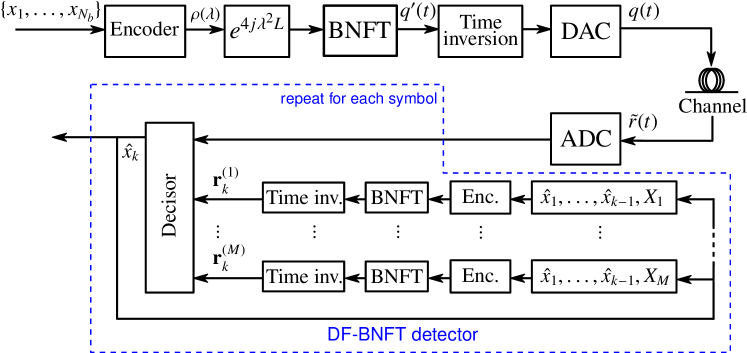
Fig. 1: NFDM with DF-BNFT detection.

The transmission scheme considered in this work is sketched in Fig. 1. As in the NIS scheme [2], the transmitter (TX) encodes a burst of $N_{b}$ symbols $\{x_{1},\ldots,x_{N_{b}}\}$ drawn from an $M$-ary quadrature amplitude modulation (QAM) alphabet $\{X_{1},\ldots,X_{M}\}$ onto a QAM signal

$$s(t)=\sum_{k=1}^{N_{b}}x_{k}g[t-(k-1)T_{s}]$$ (3)

with pulse shape $g(t)$ and symbol time $T_{s}$. In this work, for reasons that will be clarified later, we restrict $g(t)$ to have a finite duration $T\leq T_{s}$. The ordinary Fourier transform $S(f)$ of (3) is then mapped on the continuous part of the nonlinear spectrum $\rho(\lambda)$ according to

$$\rho(\lambda)=-S(-\lambda/\pi).$$ (4)

Furthermore, before computing the BNFT, deterministic propagation effects (dispersion and nonlinearity) are precompensated by multiplying the nonlinear spectrum by $\exp(j4\lambda^{2}L)$, where $L$ is the link length. Finally, the input optical signal is taken to be $q(t)=q^{\prime}(-t)$, where $q^{\prime}(t)$ is the BNFT of the precompensated nonlinear spectrum.

There are two differences between the TX described here and the one in [2], which, however, do not change the overall NIS working principle. Firstly, propagation effects are removed at the TX (precompensation) rather than at the receiver (RX). While both solutions are feasible (and splitting the compensation between TX and RX might even be advantageous [9]), precompensation is considered here because the proposed DF-BNFT detection strategy relies on it. Indeed, Corollary 3, on which DF-BNFT is based (as explained in the following), applies only to optical signals unaffected by propagation effects. Precompensation ensures that the received signal meet this requirement. Secondly, in this work each burst in the optical signal is inverted in time just to help explaining the working principle, not because it is necessary. Finally, for the sake of simplicity, we avoid explicitly mentioning the normalization and denormalization procedures required to relate the normalized signals $q(t)$ and $\tilde{r}(t)$ (see Fig. 1) to the physical signals propagating in a real fiber link, therefore assuming that the channel is characterized by the normalized version of the nonlinear Schrödinger equation (NLSE) given in [5].

Let us denote by $r(t)$ the optical signal obtained by propagating $q(t)$ in a noiseless channel. In this case, the only channel effect is the multiplication of the nonlinear spectrum by $\exp(-j4\lambda^{2}L)$, so that $r^{\prime}(t)=r(-t)$ would be the BNFT of $\rho(\lambda)$, the nonlinear spectrum before precompensation.

Corollary 2.

Considering a NIS modulation, the above optical signal $r(t)$ for $t\leq\tau$ depends only on the values of the QAM signal $s(t)$ for $t\leq\tau$.

Proof.

Taking into account (2), (3) and (4), we have that $F(y)=-s(-y/2)/2$ and thus, $F(y)$ for $y\geq 2\tau$ depends only on the values of $s(t)$ for $t\leq-\tau$. Therefore, recalling that $r^{\prime}(t)$ is the BNFT of $\rho(\lambda)$, the NFT causality property (Proposition 1) implies that $r^{\prime}(t)$ for $t\geq\tau$ depends only on $s(t)$ for $t\leq-\tau$. Changing the sign of $\tau$, one obtains that $r^{\prime}(t)$ for $t\geq-\tau$ depends only on $s(t)$ for $t\leq\tau$. Finally, the thesis follows considering that $r(t)=r^{\prime}(-t)$. ∎

Corollary 3.

Let $t_{k}=(k-1/2)T_{s}$. If the pulse shape $g(t)$ in (3) has finite duration $T\leq T_{s}$, for $t\leq t_{k}$ the optical signal $r(t)$ depends only on the symbols $x_{1},..,x_{k}$, and not on the following ones $x_{k+1},..,x_{N_{b}}$, as shown in Fig. 2. In mathematical formulas

$$r(t)\bigl{|}_{t\leq t_{k}}=\mathcal{G}\left\{x_{1},..,x_{k}\right\},$$ (5)

where $\mathcal{G}$ is a generic function.

Proof.

With this hypothesis, $s(t)$ depends only on the symbols $x_{1},\ldots,x_{k}$ for $t\leq t_{k}$. Then, applying Corollary 2, the thesis follows. ∎

Fig. 2: The NFT causality property for NIS with no ISI on $s(t)$. A train of Gaussian pulses, modulated by 16QAM symbols, and almost ISI-free, is shown before (on the left) and after (on the right) the BNFT. The red signal is generated by $8$ symbols, while for the blue one only the first $6$ are taken into account. The two optical signals are superimposed for $t\leq t_{6}$, as for Eq. (5) (baudrate $R_{s}=50\,\mathrm{GBd}$, optical power $P_{s}=7\,\mathrm{dBm}$).

4 Decision-feedback BNFT detection

In conventional NIS, the RX recovers a noisy version of the transmitted nonlinear spectrum $\rho(\lambda)$ by computing the FNFT of the received optical signal, and then makes decisions based on standard matched filtering and symbol-by-symbol detection. The improved detection scheme proposed in this work originates from the idea that, since a detrimental signal-noise interaction takes place when computing the FNFT of the received noisy signal, decisions could be alternatively made by comparing the received signal with the BNFT of all possible transmitted (noiseless) waveforms, thus avoiding signal-noise interaction effects. Selecting the waveform (and the corresponding symbols) closest to the received optical signal would correspond to a maximum a posteriori probability (MAP) strategy, under the assumption that the accumulated optical noise can be modeled as additive white gaussian noise (AWGN) (more on this later). The drawback of a sequence—rather than symbol-by-symbol—detection strategy, is an exponential growth of the detector complexity with the burst length $N_{b}$. In order to avoid this growth, the NFT causality property and a decision-feedback scheme are finally employed, obtaining the DF-BNFT detection scheme depicted in Fig. 1.

Having in mind that NIS performance decay is caused by the detection strategy itself, rather than signal-noise interaction during propagation—as also hinted by the fact that the performance obtained by simply adding AWGN after noiseless propagation is superimposed with that of the actual optical link [9]—the aim of this work is to devise a detection strategy at least optimal for the AWGN channel. Therefore, assuming the channel as AWGN, we can write the received noisy optical signal as

$$\tilde{r}(t)=r(t)+n(t),$$ (6)

where $r(t)$ is, as before, the optical signal obtained by propagating the input signal $q(t)$ in a noiseless channel, and $n(t)$ is circularly-symmetric complex white Gaussian noise with power spectral density $N_{0}$. We would like to stress that (6) is only an ansatz and not an actual identity.

An analog-to-digital converter (ADC) recovers the samples of the received noisy optical signal and collects them in the vector $\tilde{\boldsymbol{r}}$. The ADC is modeled as a rectangular filter with bandwidth $\nu/(2T_{s})$ that acquires $\nu$ samples per symbol time. Assuming that the filter bandwidth is larger than the overall signal bandwidth, under the AWGN assumption (6), $\tilde{\mathbf{r}}$ is a sufficient statistic and we can write $\tilde{\boldsymbol{r}}=\boldsymbol{r}+\boldsymbol{n}$, where $\boldsymbol{r}$ is a vector collecting the samples of $r(t)$, and $\boldsymbol{n}$ is a vector of i.i.d. circularly-symmetric complex Gaussian r.v.s $n_{k}$, with zero mean and variance $\sigma^{2}=E\{|n_{k}|^{2}\}=N_{0}\nu/T_{s}$. Therefore, conditional on $\boldsymbol{r}$, the components of $\tilde{\boldsymbol{r}}$ are independent. For the sake of simplicity, let $\tilde{\boldsymbol{r}}_{k}$ (and $\boldsymbol{r}_{k}$) be the vector of length $\nu$ representing the noisy optical signal (and, respectively, its noise-free equivalent) in the time window $[t_{k-1},t_{k})$. Hence, $\tilde{\boldsymbol{r}}$ can also be written as a compound vector $\tilde{\boldsymbol{r}}=(\tilde{\boldsymbol{r}}_{1},\ldots,\tilde{\boldsymbol{r}}_{N_{b}})$ containing the samples of the received signal in $[-T_{s}/2,(N_{b}-1/2)T_{s})$, i.e., the time window of duration $N_{b}T_{s}$ in which information is encoded. Indeed, with respect to the QAM signal $s(t)$, the optical signal after the GLME broadens in time, developing a sort of right tail that extends outside the considered detection window, i.e., for $t>(N_{b}-1/2)T_{s}$, as shown for instance in Fig. 2. Therefore, a longer vector $\tilde{r}$ should be considered to obtain a sufficient statistic. However, in the decision-feedback strategy derived in the following, this tail could be used only to detect the last symbol $x_{N_{b}}$ of the sequence, with a negligible contribution to the overall performance. Hence, for the sake of simplicity, we simply discard it.

According to the MAP strategy, and assuming equally likely input symbols, optimal detection maximizes the probability density function (pdf) $p(\tilde{\boldsymbol{r}}|\boldsymbol{x})$ of the vector $\tilde{\boldsymbol{r}}$ conditional upon the transmitted sequence $\boldsymbol{x}=(x_{1},..,x_{N_{b}})$. Thus, an optimum RX chooses the sequence $\hat{\boldsymbol{x}}$ according to

$$\hat{\boldsymbol{x}}=\mathop{\mathrm{argmax}}_{\boldsymbol{x}}p(\tilde{\boldsymbol{r}}|\boldsymbol{x}).$$ (7)

Since, conditional upon $\boldsymbol{x}$, the components of $\tilde{\boldsymbol{r}}$ are independent, the pdf in Eq. (7) can be factorized as

$$\hat{\boldsymbol{x}}=\mathop{\mathrm{argmax}}_{\boldsymbol{x}}\prod_{k=1}^{N_{b}}p(\tilde{\boldsymbol{r}}_{k}|\boldsymbol{x})=\mathop{\mathrm{argmax}}_{\boldsymbol{x}}\sum_{k=1}^{N_{b}}\ln p(\tilde{\boldsymbol{r}}_{k}|\boldsymbol{x}),$$ (8)

where the second equality stems from the monotonic behavior of the logarithm.

The NFT property (5) implies that the signal samples in the time window $[t_{k-1},t_{k})$, i.e., those collected in $\tilde{\boldsymbol{r}}_{k}$, depend only on the symbols $(x_{1},\ldots,x_{k})$. Therefore, an optimum RX performs decisions according to

$$\hat{\boldsymbol{x}}=\mathop{\mathrm{argmax}}_{\boldsymbol{x}}\sum_{k=1}^{N_{b}}\mathrm{ln}\,p(\tilde{\boldsymbol{r}}_{k}|(x_{1},\ldots,x_{k})).$$ (9)

Since the symbols $x_{1},\ldots,x_{k}$ uniquely determine $\boldsymbol{r}_{k}$, under the AWGN assumption we have

$$p(\tilde{\boldsymbol{r}}_{k}|(x_{1},\ldots,x_{k})=\frac{1}{(\pi\sigma^{2})^{\nu}}\exp\left(-\|\tilde{\boldsymbol{r}}_{k}-\boldsymbol{r}_{k}\|^{2}/\sigma^{2}\right)$$ (10)

so that $\mathrm{ln}\,p\bigl{(}\tilde{\boldsymbol{r}}_{k}\big{|}(x_{1},\ldots,x_{k})\bigl{)}=-\nu\,\mathrm{ln}\left(\pi\sigma^{2}\right)-\|\tilde{\boldsymbol{r}}_{k}-\boldsymbol{r}_{k}\|^{2}/\sigma^{2}$. This implies that, in order to determine the optimal sequence $\hat{\boldsymbol{x}}$, all possible $M^{N_{b}}$ input sequences should be considered, which is not a viable solution. In order to avoid this exponential growth of complexity, we resort to a sub-optimal decision-feedback strategy—namely, DF-BNFT—by which symbols are decided iteratively for $k=1,\ldots,N_{b}$ as

$$\hat{x}_{k}=\mathop{\mathrm{argmax}}_{X_{i}\in\left\{X_{1},..,X_{M}\right\}}\mathrm{ln}\,p\bigl{(}\tilde{\boldsymbol{r}}_{k}|(\hat{x}_{1},...,\hat{x}_{k-1},X_{i})\bigr{)}$$ (11)

bringing down to $M\times N_{b}$ the number of sequences to be considered. Equation (11) can be evaluated comparing the (samples of the) received signal with (the samples of) $M$ trial waveforms $r_{k}^{(i)}(t)$ uniquely corresponding to the sequences $\hat{x}_{1},...,\hat{x}_{k},X_{i}$ for each $X_{i}$ in the symbol constellation $\{X_{1},..,X_{M}\}$. The waveform $r_{k}^{(i)}(t)$ is obtained from the symbol sequence $\hat{x}_{1},...,\hat{x}_{k},X_{i}$ by the same encoding technique used at the TX, except for precompensation. Let $\boldsymbol{r}_{k}^{(i)}$ denote the vector of length $\nu$ containing the samples of $r_{k}^{(i)}(t)$ in $[t_{k-1},t_{k})$, referred to as detection window. In other words, $\boldsymbol{r}_{k}^{(i)}$, $i=1,\ldots,M$, are all possible vectors $\boldsymbol{r}_{k}$ given that the sequence $\hat{x}_{1},...,\hat{x}_{k},X_{i}$ has been sent. The RX implements the DF-BNFT strategy through $N_{b}$ steps as follows.

For $k=1,\ldots,N_{b}$:

• Digitally obtain the vectors $\boldsymbol{r}_{k}^{(i)}$, for each $X_{i}$ in the symbol constellation $\{X_{1},..,X_{M}\}$.

• Choose $\hat{x}_{k}$ by the rule

  $$\hat{x}_{k}=\mathop{\mathrm{argmin}}_{X_{i}\in\{X_{1},..,X_{M}\}}\bigl{\|}\tilde{\boldsymbol{r}}_{k}-\boldsymbol{r}_{k}^{(i)}\bigr{\|}^{2}$$ (12)

  where this last equation follows from (10) and (11).

The DF-BNFT strategy (11) avoids any ISI thanks to decision feedback, which accounts for the dependence of $\tilde{\mathbf{r}}_{k}$ on previous symbols, and to Corollary 3, which ensures that $\tilde{\mathbf{r}}_{k}$ does not depend on next symbols. However, it is still suboptimal compared to (9) for two reasons. The first reason is that it does not exploit the information about $x_{k}$ that is contained in the received signal after $t_{k}$. In fact, as shown in Fig. 2, while in the original QAM signal $s(t)$ (on the left) the information about $x_{k}$ is fully contained in the time interval $[t_{k-1},t_{k})$, in the corresponding optical signal $r(t)$ (on the right) part of this information goes to times $t>t_{k}$, the effect becoming more relevant with power and as $k$ increases. An apparent consequence of this effect is that the optical signal $r(t)$ has an average amplitude that decreases with time and a sort of “tail” that extends beyond the duration of the original QAM signal. The second reason is that it is affected by error propagation, as previous decisions $\hat{x}_{1},...,\hat{x}_{k-1}$ might be incorrect, this effect becoming more relevant as $k$ increases, too. Finally, even the strategy (9), that is optimal for the AWGN channel (6), might be suboptimal on a real fiber link. The effects of error propagation, information loss, and non-AWGN channel statistics are discussed in more detail in Section 6.

While the DF-BNFT strategy is conceived to improve system performance (as it will be verified in Section 6), it also has some drawbacks compared to the FNFT strategy. Firstly, to fulfill the hypothesis of Corollary 3 and avoid ISI, the pulse shape must be fully confined within a symbol time—a more stringent requirement compared to the conventional Nyquist criterion. This imposes the use of pulses with a wider bandwidth, which has a negative impact on the achievable spectral efficiency. Secondly, full channel precompensation is required to use Corollary 3 at the RX, and, therefore, channel compensation cannot be split between RX and TX to reduce guard intervals [9, 4]. Thirdly, as far as it concerns computational complexity, the DF-BNFT scheme requires the evaluation of $M$ BNFTs over $\nu N_{b}$ points. On the other hand, standard NIS detection computes only one FNFT over a comparable number of points. While an exact comparison between the two strategies depends on the relative complexity and accuracy of the considered BNFT and FNFT algorithms, it is reasonable to assume that the complexity of the DF-BNFT detector is considerably higher than that of standard FNFT detection. However, the aim of this work is to show that standard FNFT detection is far from being optimal, and that a significant increase of performance can be achieved by an improved detection strategy.

5 Error probability estimation and bounds

For a given sequence, the probability of error $P_{e}$ of the DF-BNFT strategy can be evaluated by averaging (over all constellation symbols and symbols within a burst) the probability $P_{k}^{(m)}$ that an error occurs when the symbol $X_{m}$ is sent at position $k$, provided that the symbols $\hat{x}_{1},..\hat{x}_{k-1}$ are correctly detected. Specifically,

$$P_{e}=\frac{1}{MN_{b}}\sum_{k=1}^{N_{b}}\sum_{m=1}^{M}P_{k}^{(m)}.$$ (13)

As computing $P_{k}^{(m)}$ may be difficult, we will bound it through standard techniques [11]. By defining the events $E_{m,i}=\{\text{$X_{i}$ is preferred to $X_{m}$ when deciding on $x_{k}$}\}$ and

$$E_{m}=\{\text{$X_{m}$\ is not preferred when deciding on $x_{k}$}\}=\bigcup\nolimits_{\begin{subarray}{c}i=1\\ i\neq m\end{subarray}}^{M}E_{m,i}$$ (14)

we can upper bound $P_{k}^{(m)}$ by the union bound

$$P_{k}^{(m)}=P\left(E_{m}\bigm{|}(\hat{x}_{1},...,\hat{x}_{k-1},X_{m})\right) =P\left(\bigcup\nolimits_{\begin{subarray}{c}i=1\\ i\neq m\end{subarray}}^{M}E_{m,i}\Bigm{|}(\hat{x}_{1},...,\hat{x}_{k-1},X_{m})\right)$$

$$\leq\sum_{\begin{subarray}{c}i=1\\ i\neq m\end{subarray}}^{M}P\left(E_{m,i}\Bigm{|}(\hat{x}_{1},...,\hat{x}_{k-1},X_{m})\right)$$ (15)

Due to our AWGN assumption, the pairwise error probabilities in (15) are given by

$$P\left(E_{m,i}\Bigm{|}(\hat{x}_{1},...,\hat{x}_{k-1},X_{m})\right)=\mathcal{Q}\left(\frac{d_{k}^{(m,i)}}{2\sigma}\right)$$ (16)

where

$$d_{k}^{(m,i)}=\bigl{\|}\boldsymbol{r}_{k}^{(m)}-\boldsymbol{r}_{k}^{(i)}\bigr{\|}$$ (17)

is the Euclidean distance between $\boldsymbol{r}_{k}^{(m)}$ and $\boldsymbol{r}_{k}^{(i)}$, and $\mathcal{Q}(x)\triangleq\int_{x}^{\infty}e^{-t^{2}/2}\,\mathrm{d}t/\sqrt{2\pi}=\mathop{\mathrm{erfc}}\nolimits(x/\sqrt{2})/2$ is the Q-function. We can also obtain a useful approximation on $P_{k}^{(m)}$ as follows. Denoting by $C_{m,i}$ the event complementary to $E_{m,i}$, we have

$$P_{k}^{(m)}=P\left(\bigcup\nolimits_{\begin{subarray}{c}i=1\\ i\neq m\end{subarray}}^{M}E_{m,i}\Bigm{|}(\hat{x}_{1},...,\hat{x}_{k-1},X_{m})\right)=1-P\left(\bigcap\nolimits_{\begin{subarray}{c}i=1\\ i\neq m\end{subarray}}^{M}C_{m,i}\Bigm{|}(\hat{x}_{1},...,\hat{x}_{k-1},X_{m})\right)$$ (18)

and, taking into account that $P\bigl{(}C_{m,i}\bigm{|}(\hat{x}_{1},...,\hat{x}_{k-1},X_{m})\bigr{)}=1-P\bigl{(}E_{m,i}\bigm{|}(\hat{x}_{1},...,\hat{x}_{k-1},X_{m})\bigr{)}$,

$$P_{k}^{(m)}\simeq 1-\prod_{\begin{subarray}{c}i=1\\ i\neq m\end{subarray}}^{M}\Bigl{(}1-P\left(E_{m,i}\bigm{|}(\hat{x}_{1},...,\hat{x}_{k-1},X_{m})\right)\Bigr{)}$$ (19)

where the approximation is due to the fact that, in general, the events $C_{m,i}$ are not mutually independent. Let us now derive a lower bound. Recalling that the probability of a union of events is lower bounded by each one of the probabilities of the single events, we have

$$P_{k}^{(m)}=P\left(\bigcup\nolimits_{\begin{subarray}{c}i=1\\ i\neq m\end{subarray}}^{M}E_{m,i}\Bigm{|}(\hat{x}_{1},...,\hat{x}_{k-1},X_{m})\right)\geq\max_{i\neq m}P\left(E_{m,i}\bigm{|}(\hat{x}_{1},...,\hat{x}_{k-1},X_{m})\right).$$ (20)

In conclusion, from (15), (19), (20), and taking into account (16), we have the following upper bound, approximation and lower bound, respectively, on $P_{k}^{(m)}$

$$P_{k}^{(m)} \leq\sum_{\begin{subarray}{c}i=1\\ i\neq m\end{subarray}}^{M}\mathcal{Q}\left(\frac{d_{k}^{(m,i)}}{2\sigma}\right)$$ (21)

$$P_{k}^{(m)} \simeq 1-\prod_{\begin{subarray}{c}i=1\\ i\neq m\end{subarray}}^{M}\left(1-\mathcal{Q}\left(\frac{d_{k}^{(m,i)}}{2\sigma}\right)\right)$$ (22)

$$P_{k}^{(m)} \geq\mathcal{Q}\left(\frac{d_{k}}{2\sigma}\right)$$ (23)

where

$$d_{k}=\min_{i\neq m}d_{k}^{(m,i)}$$ (24)

and $d_{k}^{(m,i)}$ is as in (17). Replacing (21)–(23) into (13) gives the corresponding bounds and approximation on $P_{e}$. We remark that both the bounds and the approximation were derived by assuming that the channel is AWGN and that previous decisions are correct. Deviations from this ideal situation might invalidate the bounds and slightly reduce the accuracy of the approximation, as shown in Section 7 by numerical simulations.

The above estimates of the probability of error for a given sequence should be averaged over all possible $M^{N_{b}}$ sequences to obtain the average error probability. However, to speed up computation, one can think of averaging over randomly generated sequences until the result stabilizes. As we will show in Section 7, this practical approach still provides a reasonable accuracy and a significant computational saving compared to direct error counting.

6 System performance

We simulated the system described in the previous sections and sketched in Fig. 1 by using a 16QAM signal $s(t)$ with symbol rate $R_{s}=1/T_{s}=50\,\mathrm{GBd}$. To fulfill the no-ISI requirement on $s(t)$, the supporting pulse was chosen to be $g(t)=\exp\bigl{(}-12.5(t/T_{s})^{2}\bigr{)}$, i.e., a Gaussian pulse with a full width at half maximum (FWHM) of $(2/5)\sqrt{2\ln 2}\,T_{s}\simeq T_{s}/2$, so that about $99.9\%$ of the energy of a pulse is contained in a symbol time. This pulse shape is chosen to fulfill the requirement of Corollary 3 on the duration of $g(t)$ with only a moderate bandwidth increase compared to the root-raised-cosine pulse employed in [9]. Note that, by relaxing the energy constraint, the bandwidth could be further reduced to approach the one in [9]. This, however, would also reduce the performance due to the ISI generated by the pulse tail, with an overall effect on the achievable spectral efficiency that should be carefully considered. The optimization of the pulse shape for the maximization of the spectral efficiency is outside the scope of this work and will be addressed in a future publication. A typical example of generated signal is shown in Fig. 2 on the left.

The channel is a standard single-mode fiber of length $L=2000\,\mathrm{km}$ with group velocity dispersion (GVD) parameter $\beta_{2}=-20.39\,\mathrm{ps^{2}/km}$, nonlinear coefficient $\gamma=1.22\,\mathrm{W^{-1}km^{-1}}$, and attenuation $\alpha=0.2\,\mathrm{dB/km}$. Ideal distributed amplification (spontaneous emission factor $\eta_{\mathrm{sp}}=4$) is considered along the channel. The bandwidth of both the digital-to-analog converter (DAC) and the ADC is $100\,\mathrm{GHz}$. In order to account for the NFT boundary conditions and for temporal broadening due to dispersion, a total of $N_{z}=2000$ guard symbols is considered in our simulations. The FNFT and BNFT operations are performed considering an oversampling factor of $8$ samples per symbols, respectively using the Layer-Peeling (LP) method [1] and an enhanced version of the Nystrom method [12]. The simulation results are deemed free from numerical inaccuracies, since it was verified that the noise-free performance was sufficiently higher than the noisy one (when applicable), and that higher accuracy did not change the results, similarly to what done in [13].

As often customary in optical communications, performance is measured in terms of Q-factor, defined as $Q_{\mathrm{dB}}^{2}=20\log_{10}[\sqrt{2}\mathop{\mathrm{erfc}}\nolimits^{-1}(2P_{b})]$, where the probability of bit error $P_{b}$ is given by direct error counting [14]. The rate efficiency $\eta=N_{b}/(N_{b}+N_{z})$ is considered to account for the spectral efficiency loss due to the insertion of guard symbols [9]. The performance is reported as a function of the mean power per symbol, defined as $P_{s}=E_{s}/T_{s}$, where $E_{s}=E_{\mathrm{tot}}/N_{b}$ is the mean energy per information symbol and $E_{\mathrm{tot}}$ the total energy of the optical signal (so that the actual average optical power is $\eta P_{s}$).

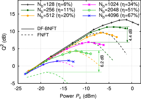
Fig. 3: Performance of the NFDM system for DF-BNFT (solid lines) and standard FNFT (dashed lines) detection for different burst length $N_{b}$ (and rate efficiency $\eta$). $16$QAM symbols, $\beta_{2}=-20.39\,\mathrm{ps^{2}/km}$, $N_{z}=2000$, $L=2000\,\mathrm{km}$, and $R_{s}=50\,\mathrm{GBd}$.

Figure 3 shows the NFDM performance obtained with DF-BNFT detection (solid lines), and with conventional FNFT (dashed lines), for different burst lengths (same color for same length). As can be seen, the performance obtained with DF-BNFT is significantly better than that obtained with FNFT detection, with an improvement of $4.4$ dB for $N_{b}=256$ and $6.2$ dB for $N_{b}=2048$. However, performance still decays when increasing $N_{b}$. This behavior may be due either to the suboptimality of the DF-BNFT detection, or to an intrinsic limitation of the NIS modulation format. For what concerns suboptimality, there are three possible causes of performance degradation, already discussed in Section 4: the non-AWGN statistics of the fiber channel, which is affected by signal-noise interaction; the error propagation in the decision-feedback mechanism of (11); and the information loss entailed by (12), which neglects the information about $x_{k}$ that is contained in the received signal for $t>t_{k}$. All these effects become more relevant as the burst length increases. Also signal-noise interaction increases with the burst length, as the optical noise interacts with a longer portion of non-zero signal. This effect, however, saturates when the burst length becomes longer than the channel memory. One may wonder whether the NIS performance shown here is in accordance with the theoretical estimation of the signal to noise ratio (SNR) given in [15]. Such a comparison was performed in [9] for almost the same system configuration considered here. The only differences are: (1) the modulation format, which however does not significantly change the results, and (2) the chosen pulse shape. In this work, a pulse with a shorter time duration and, hence, a wider bandwidth is considered. This difference is responsible for a slight performance improvement.

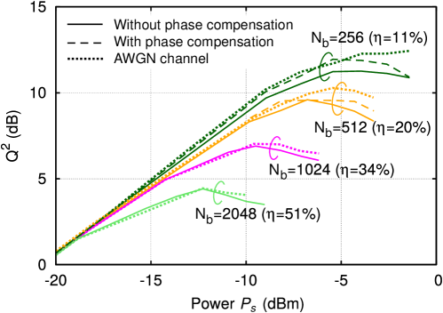
Fig. 4: Impact of fiber propagation: performance of DF-BNFT on the fiber link without (solid lines) and with average nonlinear phase compensation (dashed lines) and on the AWGN channel (dotted line). Same scenario of Fig. 3.

The impact of signal-noise interaction during propagation can be estimated by comparing the performance obtained on the fiber link with the performance obtained on the corresponding AWGN channel, shown in Fig. 4 with dotted lines for $N_{b}=256,\,512,\,1024,\,2048$. For longer bursts, i.e., $N_{b}\geq 1024$, the corresponding dotted and solid lines are almost indistinguishable. On the other hand, for shorter bursts, i.e., $N_{b}=256,\,512$, the slight difference between the dotted and solid lines denotes a small impact of signal-noise interaction on system performance and a slight deviation of channel statistics from the AWGN assumption (6). One of the effects of signal-noise interaction during propagation is a constant phase rotation of the optical signal. This deviation can be estimated and removed from the optical signal considering for detection $\tilde{r}(t)e^{-j\alpha}$, $\alpha$ being the phase shift, rather than $\tilde{r}(t)$ itself. Fig. 4 shows that a small performance gain can be obtained with this technique (performance shown with dashed lines) and that the performance approaches those of the equivalent AWGN channel. Obviously, when performance is superimposed to that of the AWGN channel, this technique does not affect the detection strategy.

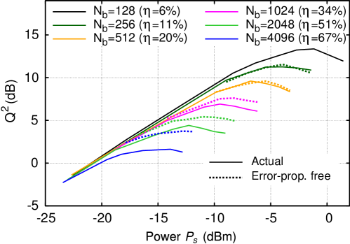
Fig. 5: Impact of error propagation due to decision feedback in the proposed DF-BNFT detection strategy: actual performance (solid lines), and error-propagation-free performance (dotted lines). Same scenario of Fig. 3.

As regards error propagation, its impact can be estimated from Fig. 5, in which the actual DF-BNFT performance is compared to that of an ideal detector that makes decisions according to the same strategy (11), but using the correct symbols $x_{1},\ldots,x_{k-1}$ rather than the detected ones $\hat{x}_{1},\ldots,\hat{x}_{k-1}$. Contrarily to what observed for signal-noise interaction, the impact of error propagation is more relevant for longer bursts, while it tends to be negligible for shorter ones. Indeed, for longer bursts, farther symbols (i) affect more significantly detection, and (ii) are more likely to be wrong, since the probability of error is higher.

As regards the third possible cause of performance degradation, further investigations are required to estimate the impact of information loss due to the suboptimality of (11) and to devise a better strategy to avoid it. Eventually, the implementation of an optimal strategy based on (9), but with a feasible complexity, would allow to estimate the ultimate performance of NIS modulation and to understand if the observed performance decay is due to suboptimal detection or to an intrinsic limitation of this modulation scheme. This is currently under investigation.

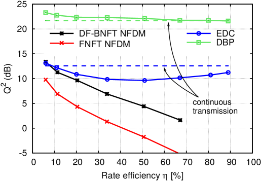
Fig. 6: Best achievable performance vs rate efficiency for NFDM with different detection strategies and for conventional systems with EDC or DBP. Same scenario of Fig. 3.

The maximum performance achieved by FNFT and DF-BNFT detection (at their respective optimum power) in Fig. 3 are reported in Fig. 6 as a function of the rate efficiency and compared with the maximum performance achieved by conventional systems (also operating in burst mode, for a fair comparison) employing ideal electronic dispersion compensation (EDC) and digital backpropagation (DBP) (practically implemented by the split-step Fourier method with $100$ steps per span of fiber, enough to practically achieve a perfect compensation of deterministic nonlinearity). DBP performance is estimated from the error vector magnitude [16], rather than calculated by direct error counting, being the corresponding error probability too low to be measured. The improvement of DF-BNFT with respect to FNFT is quite relevant and slightly increases with the rate efficiency $\eta$. However, the DF-BNFT performance is still not on par with that of conventional systems and keeps decreasing at higher rates, when the performance of conventional systems saturate to the one achieved with continuous (non burst mode) transmission. Finally, the performance achievable by DF-BNFT detection was investigated also in different scenarios. Fig. 7a refers to the same system setup used in Figs. 3–6 but with a lower dispersion parameter $\beta_{2}=-1.27\,\mathrm{ps^{2}/km}$ and, therefore, a lower number of guard symbols $N_{z}=125$. The overall results do not change significantly, as already observed in [9], and DF-BNFT achieves a performance improvement of almost $6$ dB with respect to FNFT detection. The behavior also does not change when using quadrature phase-shift keying (QPSK) symbols in the otherwise same system of Fig. 3 but with lower symbol rate $R_{s}=10\,\mathrm{GBd}$, longer link length $L=4000\,\mathrm{km}$, and $N_{z}=160$ guard symbols, as shown in Fig. 7b.

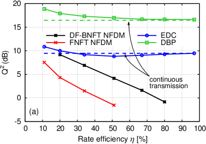
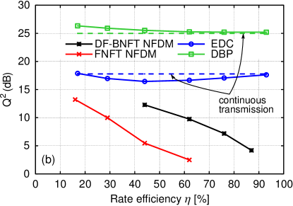
Fig. 7: Best achievable performance vs rate efficiency for NFDM with different detection strategies and for conventional systems with EDC or DBP: (a) low-dispersion fiber with $16$QAM symbols, $\beta_{2}=-1.27\,\mathrm{ps^{2}/km}$, $N_{z}=125$, $L=2000\,\mathrm{km}$, and $R_{s}=50\,\mathrm{GBd}$; (b) QPSK symbols with $\beta_{2}=-20.39\,\mathrm{ps^{2}/km}$, $N_{z}=160$, $L=4000\,\mathrm{km}$, and $R_{s}=10\,\mathrm{GBd}$.

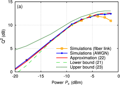
Fig. 8: Validation of the semianalytic approximation and bounds for the performance of DF-BNFT detection. Same scenario of Fig. 3, with (a) $N_{b}=256$ and (b) $N_{b}=1024$.

7 Validation of the approximation and bounds

The bounds and approximation obtained by replacing (21)–(23) into (13) are reported in Fig. 8 for $N_{b}=256$ and $N_{b}=1024$, after conversion to Q-factor. As the Q-factor is directly related to the bit-error probability $P_{b}$, the approximation $P_{b}\simeq P_{e}/M$ is used, assuming that a symbol error always corresponds to a single bit error. Moreover, if $P_{e}$ increases, the $Q$ factor decreases, and the other way around. Therefore a lower (or upper) bound for $P_{e}$ becomes an upper (or lower) bound for $Q_{\mathrm{dB}}^{2}$. In order to check their accuracy, they are compared with the performance obtained by numerical simulations for the actual fiber channel. In both cases, the approximation lies between the bounds, asymptotically approaching the lower bound when power increases. At low powers, the approximation is in very good agreement with numerical simulations. On the other hand, near the optimum power, the approximation overestimates the actual performance, which falls slightly below the lower bound. This is due to signal-noise interaction during propagation (for $N_{b}=256)$ and to error propagation in the decision-feedback strategy (for $N_{b}=1024)$, both neglected in the derivation of the bounds and approximation (21)–(23). In fact, when considering the numerical simulations for the AWGN channel in Fig. 8a, and the error-propagation-free simulations in Fig. 8b, they correctly fall between the bounds and are in excellent agreement with the approximation.

As already explained, the probability of error for a given sequence $P_{e}$ in (13) should be averaged over all possible sequences. However, the number of possible sequences $M^{N_{b}}$ is practically unmanageable, making it impossible performing an exact average. Anyway, most sequences contribute in the same way to the average, so that we don’t need to explore all of them, but only account for the most significant ones. This can be done by performing a Monte Carlo average, consisting in randomly generating sequences until the corresponding average performance stabilizes. This is in contrast with the full numerical estimation used in Section 6, in which also the effect of noise is numerically estimated by averaging over many random realizations. To illustrate the difference between the two approaches and show the speed of convergence of the various estimates, Fig. 9 reports the same bounds and estimates shown in Fig. 8a as a function of the number of iterations (corresponding to the number of sequences of length $N_{b}$ over which the performance is averaged), considering two different values of the mean power. As can be seen, the computation of the semianalytical bounds and approximation requires only a few iterations in all cases, while computing the performance by full numerical simulations requires a number of iterations that depends on the actual error probability and, hence, on the input power, such that a sufficient number of error events are observed. As an example, $30\div 40$ iterations suffice for an input power of $-9\,\mathrm{dBm}$, while more than 200 iterations are necessary at the optimum input power of $-4\,\mathrm{dBm}$.

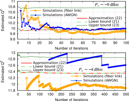
Fig. 9: Convergence of the numerical simulations and of the semianalytic approximation and bounds with the number of iterations (transmitted sequences). Same scenario of Fig. 3, with $N_{b}=256$ at $P_{s}=-9$dBm (above) and at optimal power $P_{s}=-4$dBm (below).

8 Conclusions

Differently than in conventional systems, there is still no theory for optimum detection when using the NFT as a mean to transmit information. As a result, the existing NFT-based transmission schemes mostly rely on reasonable assumptions and are guided by concepts and principles borrowed from the more familiar detection theory for linear systems. This means that big improvements are to be expected as soon as the principles of nonlinear detection theory are better understood. There is a lot still to be discovered, but some well known general principles can be applied independently of the nature of the systems at hand, be it linear or not. For example, this is the case for the MAP detection strategy to be applied in a given communication system, once a statistical knowledge of the channel is available or can be reasonably approximated.

Following this line, by assuming a simple channel model, a novel (suboptimal) detection strategy for NFDM systems, referred to as DF-BNFT, has been introduced in this work. In a nutshell, taking advantage of a peculiar property of the NFT, rather than using a strategy based on the FNFT and the minimization of the Euclidean distance in the nonlinear frequency domain, DF-BNFT takes decisions by minimizing the Euclidean distance in the time domain through BNFT and decision feedback. Moreover, a semianalytical approximation, upper and lower bounds to system performance have been derived, providing an effective tool to estimate system performance without resorting to time-consuming numerical simulations.

As demonstrated by numerical results, the proposed detection strategy allows for a performance improvement of up to $6.2$ dB with respect to standard FNFT detection. Despite such a big improvement, also the performance of the proposed DF-BNFT strategy decays when the burst length increases, similarly to what observed for FNFT-based detection [9]. This peculiar behavior forces the use of short bursts, separated by long guard times, severely limiting the overall spectral efficiency achievable by the system. However, while the performance decays in FNFT and DF-BNFT detection appear to be similar, their causes are different: the perturbation of the nonlinear spectrum caused by optical noise (and non-optimally accounted for by the detection metrics) in the former case; the information loss and error propagation caused by the use of the suboptimum strategy (11) in the latter.

Though the persistence of this undesirable behavior might be daunting, in fact making NFDM not yet competitive with conventional systems, the relevant performance improvement obtained by a still sub-optimum strategy is rather encouraging and paves the way for further progresses. Possible future developments include: the implementation of the optimum detection strategy (9) to overcome the limitations induced by (11); the reduction of computational complexity; the optimization of the pulse shape to maximize the achievable spectral efficiency; the investigation of the impact of more practical amplification schemes, such as lumped amplification, in which the lossless path-average model needs to be employed [17, 18]; and the extension of the detection strategy to the dual-polarization case. Such developments are required to fully exploit the potentials of the NFDM technique and to understand if it can provide any practical advantages compared to conventional transmission techniques.

Funding

Ente Cassa di Risparmio di Firenze.