Harmonically trapped attractive and repulsive spin-orbit and Rabi coupled Bose-Einstein condensates

Abstract

Numerically we investigate the ground state of effective one-dimensional spin-orbit (SO) and Rabi coupled two pseudo-spinor Bose-Einstein condensates (BECs) under the effect of harmonic traps. For both signs of the interaction, density profiles of SO and Rabi coupled BECs in harmonic potentials, which simulate a real experimental situation are obtained. The harmonic trap causes a strong reduction of the multi-peak nature of the condensate and it increases its density. For repulsive interactions, the increase of SO coupling results in an uncompressed less dense condensate and with increased multi-peak nature of the density. The increase of Rabi coupling leads to a density increase with an almost constant number of multi-peaks. For both signs of the interaction and negative values of Rabi coupling, the condensate develops a notch in the central point and it seems to a dark-in-bright soliton. In the case of the attractive nonlinearity, an interesting result is the increase of the collapse threshold under the action of the SO and Rabi couplings.

1 Introduction

In last few years, the creation of synthetic non-Abelian gauge fields in neutral atoms has attracted a great interest. Particularly, Lin et al. [1] accomplished the experimental realization of an artificial spin-orbit (SO) coupling in a neutral atomic Bose-Einstein condensate (BEC) by means of counterpropagating laser beams coupling two atomic spin states of ⁸⁷Rb hyperfine state 5$S_{1/2}$, $|\uparrow\rangle=|F=1,m_{F}=0\rangle$ and $|\downarrow\rangle=|F=1,m_{F}=-1\rangle$, where $F$ is the total angular momentum of the hyperfine state and $m_{F}$ is the $z$ projection of $F$. In analogy with the two spin components of a spin-half particle these states are called pseudo-spin-up and pseudo-spin-down states. This technique also has been implemented in Bose [2] and atomic Fermi gases [3]. These experimental breakthroughs have led to significant theoretical works, opening the door to a fascinating and fast development of unconventional phenomena on SO and Rabi coupled ultracold atoms research. In [4] are presented remarkable recent and ongoing realizations of Rashba physics in cold atom systems, Dirac materials, Majorana femions and beyond. Some basic aspects about quantum gases with SO coupling are introduced in [5].

The SO and Rabi coupled BECs have been studied in different contexts, solitons in one-dimensional (1D) geometries [6] and two-dimensional (2D) geometries [7], vortices with or without rotations [8]. The quantum tricriticality and the phase transitions are studied by considering a SO coupled configuration of spin-1/2 interacting bosons with equal Rashba and Dresselhaus couplings [9]. In [10] it is shown that the bosons condenses into a single momentum state of the Rashba spectrum via the mechanism of order by disorder. Stability of plane waves in a 2D SO coupled BEC was studied analytically in [11]. A study of localization of a noninteracting and weakly interacting SO coupled BEC in a quasiperiodic bichromatic optical lattice (OL) potential it was carried out in [12]. The existence of antiferromagnetically ordered (striped) ground states in a 1D SO coupled system with repulsive atomic interactions under the action of a harmonic oscillator (HO) potential it is demonstrated in [13]. The Josephson dynamics of a SO coupled BEC is investigated in [14]. There have also been efforts toward understanding SO coupling related physics at finite temperature [15]. Further, in trapped systems more intriguing ground state properties arise from the nontrivial interplay between SO coupling, confinement and inter-atomic interactions. The phase diagram includes two rotationally symmetric phases, a hexagonally symmetric phase with triangular lattice of density minima similar to that observed in rotating condensates, and a stripe phase [16]. Wang et al. have identified two different phases for the ground state of homogeneous spin-1/2 and spin-1 BECs with Rashba SO coupling [17]. From the spin-dependent interactions, the condensate is found to be a single plane wave or it is a standing wave forming spin stripes. At strong SO coupling in trapped weakly interacting BECs, the single particle spectrum decomposes into discrete manifolds and quantum states with Skyrmion lattices emerge when all bosons occupy the lowest manifold [18]. In ultracold Bose gases with Rashba SO coupling the presence of a weak harmonic potential results in a striped state with lower energy than the conventional striped state in the homogeneous scenario [19]. The ground states of a single particle, two bosons, and two fermions confined in a 1D harmonic trap with Raman-induced SO coupling are considered in [20]. The collective dynamics of the SO coupled BEC trapped in a quasi-1D harmonic potential it is studied in [21]. Recently, the influence of interaction parameters, SO and Rabi couplings on the modulation instability in a condensate it is investigated in [22]. The combined effects of SO coupling and a non-local dipolar interaction have given rise to a rich variety of ground state spin structures in a condensate [23].

At zero temperature, the time-dependent mean-field 3D Gross-Pitaevskii equation (GPE) is a good theoretical tool for the study of dilute BECs [24]. However, an interesting question is the derivation of reduced 1D and 2D models to have an insight about the behavior of the 3D full system. Experimentally these effective models are useful for testing many-body phenomena [25]. Theoretically they have been derived 1D and 2D models from the 3D GPE in different contexts of BEC research [26]. A starting point for the theoretical study of SO coupled BECs with reduced dimensionality is provided by [27], where a binary mean-field nonpolynomial Schrödinger equation (NPSE) has been used in research of localized modes in condensates. In a similar way, condensates with the SO coupling of mixed Rashba-Dresselhaus type and Rabi term are described by two coupled 2D NPSEs [28].

In this work we show the effect of harmonic traps on SO and Rabi coupled BECs. Starting from the 3D many-body Hamiltonian describing $N$ interacting bosons of equal mass with SO and Rabi couplings, we study the 1D reduction of a 3D bosonic quantum field theory. We achieve to getting two time-dependent 1D coupled nonpolynomial Heisenberg equations (NPHEs). If the many-body quantum state of the system is well-approximated to the Glauber coherent state, our findings are consistent with those obtained in a mean-field approximation [27]. This is followed by a numerical solution of the coupled NPSEs. For attractive and repulsive SO and Rabi coupled BECs we investigate some aspects of the interplay between the strength of the harmonic confinement, the SO and Rabi couplings. Our results show that the harmonic trap causes a reduction of the multi-peak nature of the condensate and it increases the density in both attractive and repulsive condensates. In the case of repulsive interactions, the increase of SO coupling results in an increased multi-peak nature of the density with a less dense condensate without its compression. The increase of Rabi coupling leads to a density increase with an almost constant number of multi-peaks. For both signs of the interaction and negative values of $\Gamma$, the condensate develops a notch in the central point and it seems to a dark-in-bright soliton [29]. A relevant finding is the increment of the strength of the attractive nonlinearity at the collapse threshold.

The rest of the paper is organized in the following way. In the Sec. 2, we derive two effective 1D coupled NPHEs and the condition under which these match the 1D NPSEs describing BECs with SO and Rabi couplings. This is followed by a discussion about some aspects related to the numerical normalization of the wave-function in Sec. 3. Numerical results of the SO and Rabi coupled BECs in harmonic traps are reported in Sec. 4. Finally, we present a summary and discussion of our study in Sec. 5.

2 Theoretical model

2.1 Coupled Nonpolynomial Heisenberg Equations

A quantum treatment of a dilute gas of $N$ interacting bosonic atoms of equal mass $m$, with SO and Rabi couplings can be obtained from the dimensionless many-body Hamiltonian given in [30]. In order to obtain this dimensionless form, it has been used the HO length of the transverse trap $a_{\perp}=\sqrt{\hbar/(m\omega_{\perp})}$, with the trapping frequency $\omega_{\perp}$. The time $t$ is measured in units of $\omega^{-1}_{\perp}$, the spatial variable ${\bf r}$ in units of $a_{\perp}$, the energy in units $\hbar\omega_{\perp}$ and the field operators are given in units of $a_{\perp}^{3/2}$. Such a Hamiltonian can be read as

$${\hat{H}} = \int d{\bf r}\sum_{j=1,2}\bigg{\{}{\hat{\psi}}_{j}^{\dagger}\bigg{[}-{\frac{1}{2}}\nabla^{2}+U(\mathbf{r})+(-1)^{j-1}i\gamma\frac{\partial}{\partial x}\bigg{]}{\hat{\psi}}_{j}$$ (1)

$$+ \Gamma{\hat{\psi}}_{j}^{\dagger}{\hat{\psi}}_{3-j}+\sum_{l=1,2}\pi g_{jl}{\hat{\psi}}_{j}^{\dagger}{\hat{\psi}}_{l}^{\dagger}{\hat{\psi}}_{j}{\hat{\psi}}_{l}\bigg{\}}$$

where ${\hat{\psi}_{j}}^{\dagger}$ and ${\hat{\psi}_{j}}$ $(j=1,2)$ are the two pseudo-spin creation and annihilation boson field operators, respectively. $g_{jj}\equiv 2a_{jj}/a_{\perp}$, and $g_{12}=g_{21}\equiv 2a_{12}/a_{\perp}$ are the strengths of the intra- and inter-species interactions, with $a_{jj}$ and $a_{12}$ the respective intra- and inter-species s-wave scattering lengths. $U\left(\mathbf{r}\right)$ is an external potential, and it is given as $U(\mathbf{r})=V(x)+(y^{2}+z^{2})/2$, where $V(x)$ is a generic potential in the $x$ axial direction and the HO potential keeps the confinement of the system in the transverse $(y,z)$ plane. $\gamma\equiv k_{L}a_{\perp}$ and $\Gamma\equiv\Omega/(2\omega_{\perp})$ are the dimensionless strengths of the SO and Rabi couplings, respectively. $k_{L}$ is the recoil wave number induced by the interaction with the laser beams and $\Omega$ is the frequency of the Raman coupling, responsible for the Rabi mixing between the two states. The bosonic field operators and their adjoints must satisfy the following equal-time commutation rules, $[{\hat{\psi}}_{\alpha}({\bf r},t),{\hat{\psi}}_{\beta}^{\dagger}({\bf r}^{\prime},t)]=\delta_{\alpha\beta}\delta({\bf r}-{\bf r}^{\prime})$ and $[{\hat{\psi}}_{\alpha}({\bf r},t),{\hat{\psi}}_{\beta}({\bf r}^{\prime},t)]=[{\hat{\psi}}_{\alpha}^{\dagger}({\bf r},t),{\hat{\psi}}_{\beta}^{\dagger}({\bf r}^{\prime},t)]=0$, where $\alpha,\beta=1,2$. The creation of a particle in the state $|{\bf r},\alpha,t\rangle$ from the vacuum state $|0\rangle$ is given as ${\hat{\psi}}_{\alpha}^{\dagger}({\bf r},t)|0\rangle=|{\bf r},\alpha,t\rangle$. The annihilation of a particle in the state $|{\bf r},\beta,t\rangle$ is given by ${\hat{\psi}}_{\alpha}({\bf r}^{\prime},t)|{\bf r},\beta,t\rangle=\delta_{\alpha\beta}\delta({\bf r}-{\bf r}^{\prime})|0\rangle$. From the Heisenberg equation of motion $i{\partial_{t}{\hat{\psi}}_{j}}=[{\hat{\psi}}_{j},{\hat{H}}]$, we get two coupled field equations in a closed form,

$$i{\frac{\partial}{\partial t}}{\hat{\psi}}_{j}(\mathbf{r},t) = \bigg{[}-{\frac{1}{2}}\nabla^{2}+V(x)+{1\over 2}\left(y^{2}+z^{2}\right)$$ (2)

$$+ (-1)^{j-1}i\gamma\frac{\partial}{\partial x}+2\pi g_{jj}{\hat{\psi}}_{j}^{\dagger}(\mathbf{r},t){\hat{\psi}}_{j}(\mathbf{r},t)$$

$$+ 2\pi g_{12}{\hat{\psi}}_{3-j}^{\dagger}(\mathbf{r},t){\hat{\psi}}_{3-j}(\mathbf{r},t)\bigg{]}{\hat{\psi}}_{j}(\mathbf{r},t)+\Gamma{\hat{\psi}}_{3-j}(\mathbf{r},t)$$

2.2 1D reduction of the 3D Hamiltonian

To perform the 1D reduction of the 3D Hamiltonian (1), we suppose that the single-particle ground state in the transverse $(y,z)$ plane is given by a Gaussian wave-function [30, 31, 32, 33], such that

$${\hat{\psi}}_{j}({\bf r})|G\rangle={1\over\sqrt{\pi}\ \eta_{j}(x,t)}\exp{\left[-{y^{2}+z^{2}\over 2\eta^{2}_{j}(x,t)}\right]}\,{\hat{\phi}}_{j}(x,t)|G\rangle\;$$ (3)

where $|G\rangle$ is the many-body ground state, while ${\hat{\phi}}_{j}(x,t)$ and $\eta_{j}(x,t)$ $(j=1,2)$ are, respectively, the axial bosonic field operators and the transverse widths. Inserting this ansatz into the Hamiltonian (1), performing the integration in the transverse plane, and neglecting derivatives of $\eta_{j}(x,t)$, one can derive the corresponding effective 1D-Hamiltonian ${\hat{h}}_{1D}$ [30], such that ${\hat{H}}|G\rangle={\hat{h}}_{1D}|G\rangle$. The tranverse widths $\eta_{j}(x,t)$ are determined by minimizing the energy functional $\langle G|{\hat{h}_{1D}}|G\rangle$ with respect to $\eta_{j}(x,t)$ [30, 32]. The ground state $|G\rangle$ is obtained self-consistently from ${\hat{h}}_{1D}$ and $\eta_{j}(x,t)$. Now, from ${\hat{h}}_{1D}$ and $i{\partial_{t}\hat{\phi}}_{j}=[{\hat{\phi}}_{j},{\hat{h}}_{1D}]$, we derive two 1D coupled NPHEs describing a many-body quantum system of dilute bosonic atoms with SO and Rabi couplings,

$$i{\partial\over\partial t}{\hat{\phi}}_{j} = \bigg{[}-{\frac{1}{2}}\frac{\partial^{2}}{\partial x^{2}}+V(x)+\frac{1}{2}\left(\frac{1}{\eta_{j}^{2}}+\eta_{j}^{2}\right)+(-1)^{j-1}i\gamma\frac{\partial}{\partial x}$$ (4)

$$+ \frac{g_{jj}}{\eta^{2}_{j}}{\hat{\phi}}_{j}^{\dagger}{\hat{\phi}}_{j}+\frac{2g_{12}}{\eta^{2}_{1}+\eta^{2}_{2}}{\hat{\phi}}_{3-j}^{\dagger}{\hat{\phi}}_{3-j}\bigg{]}{\hat{\phi}}_{j}+2\Gamma\frac{\eta_{1}\eta_{2}}{\eta_{1}^{2}+\eta_{2}^{2}}{\hat{\phi}}_{3-j}$$

This system of equations must be solved self-consistently using the many-body quantum state of the system $|S\rangle$ in the equations of the transverse widths $\eta_{j}$ [30, 32]. So

$$\eta_{j}^{4} = 1+g_{jj}\frac{\langle S|{\hat{\phi}}_{j}^{\dagger}{\hat{\phi}}_{j}^{\dagger}{\hat{\phi}}_{j}{\hat{\phi}}_{j}|S\rangle}{\langle S|{\hat{\phi}}_{j}^{\dagger}{\hat{\phi}}_{j}|S\rangle}+4g_{12}\frac{\eta_{j}^{4}}{(\eta^{2}_{1}+\eta^{2}_{2})^{2}}\frac{\langle S|{\hat{\phi}}_{1}^{\dagger}{\hat{\phi}}_{2}^{\dagger}{\hat{\phi}}_{2}{\hat{\phi}}_{1}|S\rangle}{\langle S|{\hat{\phi}}_{j}^{\dagger}{\hat{\phi}}_{j}|S\rangle}$$ (5)

$$+ 2(-1)^{j-1}\Gamma\eta_{j}^{3}\eta_{3-j}\frac{\eta_{1}^{2}-\eta_{2}^{2}}{(\eta_{1}^{2}+\eta_{2}^{2})^{2}}\frac{\langle S|({\hat{\phi}}_{1}^{\dagger}{\hat{\phi}}_{2}+{\hat{\phi}}_{2}^{\dagger}{\hat{\phi}}_{1})|S\rangle}{\langle S|{\hat{\phi}}_{j}^{\dagger}{\hat{\phi}}_{j}|S\rangle}$$

As a particular case with $\eta_{j}^{4}=1$, the model (4) describes an one-dimensional dilute gas of bosonic atoms with SO and Rabi couplings confined by a generic potential $V(x)$ in the $x$ direction.

Nevertheless, in an open environment particles may be added or removed from the system and one can suppose that the number of bosons in the matter field is not fixed, i.e. the system is not in a pure Fock state [33, 34, 35]. Then in analogy with a functional-integral formalism to investigate interacting quantum gases [35] and the description in optics of a radiation field of a laser device operating in a single mode [36], we introduce the Glauber coherent state $|GCS\rangle$, which does not have a fixed number of particles. This coherent state is defined as an eigenstate of the annihilation operator. In terms of quantum field operators we have ${\hat{\phi}}_{j}(x,t)|GCS\rangle=\phi_{j}(x,t)|GCS\rangle$ where $\phi_{j}(x,t)$ is a classical field, and the average number of atoms in the coherent state is given as $N_{j}=\langle GCS|\hat{N}_{j}|GCS\rangle$. Hence, when the many-body quantum state $|S\rangle$ is considered as a Glauber coherent state $|GCS\rangle$ [31, 32, 33], the 1D NPHE (4) becomes 1D NPSE [27, 30]

$$i{\partial\over\partial t}\phi_{j} = \bigg{[}-{\frac{1}{2}}\frac{\partial^{2}}{\partial x^{2}}+V(x)+\frac{1}{2}\left(\frac{1}{\eta_{j}^{2}}+\eta_{j}^{2}\right)+(-1)^{j-1}i\gamma\frac{\partial}{\partial x}$$ (6)

$$+ \frac{g_{jj}}{\eta^{2}_{j}}\left|\phi_{j}\right|^{2}+\frac{2g_{12}}{\eta^{2}_{1}+\eta^{2}_{2}}\left|\phi_{3-j}\right|^{2}\bigg{]}\phi_{j}+2\Gamma\frac{\eta_{1}\eta_{2}}{\eta_{1}^{2}+\eta_{2}^{2}}\phi_{3-j}$$

The time-dependent spinor complex wave-functions $\phi_{j}$ $(j=1,2)$ describe the two pseudo-spin components $|\uparrow\rangle$ and $|\downarrow\rangle$, respectively. The normalization conditions are given by $\int_{-\infty}^{\infty}dx|\phi_{j}(x,t)|^{2}=N_{j}$, where $N_{j}$ is the number of atoms in the $j$ component, and the conserved total number of atoms is $N=N_{1}+N_{2}$. The corresponding transverse widths (5), become

$$\eta_{j}^{4} = 1+g_{jj}\left|\phi_{j}\right|^{2}+4g_{12}\frac{\eta_{j}^{4}}{(\eta^{2}_{1}+\eta^{2}_{2})^{2}}\left|\phi_{3-j}\right|^{2}$$ (7)

$$+ 2(-1)^{j-1}\Gamma\eta_{j}^{3}\eta_{3-j}\frac{\eta_{1}^{2}-\eta_{2}^{2}}{(\eta_{1}^{2}+\eta_{2}^{2})^{2}}\frac{(\phi_{1}^{*}\phi_{2}+\phi_{2}^{*}\phi_{1})}{\left|\phi_{j}\right|^{2}}$$

In general, the coupled Eqs. (6) are strictly 1D under the condition $\eta_{j}^{4}=1$ in the system of Eqs. (7), establishing the conventional 1D GPE with SO and Rabi couplings

$$i{\partial\over\partial t}\phi_{j} = \bigg{[}-{\frac{1}{2}}\frac{\partial^{2}}{\partial x^{2}}+V(x)+(-1)^{j-1}i\gamma\frac{\partial}{\partial x}$$ (8)

$$+ g_{jj}\left|\phi_{j}\right|^{2}+g_{12}\left|\phi_{3-j}\right|^{2}\bigg{]}\phi_{j}+\Gamma\phi_{3-j}$$

we have omitted the constant contribution of the transverse energy given as $1$ (in units of $\omega_{\perp}$). This model becomes the one that it was implemented to studying nonlinear modes in binary bosonic condensates with nonlinear repulsive interactions and linear SO- and Zeeman-splitting couplings [13]. For this purpose, it is necessary to use the transformations $(-1)^{j-1}\partial_{x}\phi_{j}\rightarrow\partial_{x}\phi_{3-j}$ and $\phi_{3-j}\rightarrow(-1)^{j+1}\phi_{j}$, which are tantamount to the global pseudo-spin rotations $\sigma_{x}\rightarrow\sigma_{z}$ and $\sigma_{z}\rightarrow\sigma_{x}$ given in [30]. Another useful conserved quantity relating the two components of the density is the pseudo-magnetization density $\mathcal{M}$ defined as $\mathcal{M}\equiv N^{-1}\left(|\phi_{1}(x)|^{2}-|\phi_{2}(x)|^{2}\right)$ [13, 38], with the respective total pseudo-magnetization $M=\int_{-\infty}^{\infty}dx\mathcal{M}$. The conserved total number of atoms and the conserved total pseudo-magnetization are considered as constraints to compute the ground state of SO and Rabi coupled BECs as it is discussed in Sec. 3.

The above models (6) and (7) were previously derived in a mean-field approximation describing a BEC with pseudo-spin states $|\uparrow\rangle$ and $|\downarrow\rangle$ [27]. In this approximation the number of atoms in the single-particle condensed state is considered large and the quantum fluctuations are negligible so that the Bogoliubov approximation can be used [24]. Indeed our results let see the correspondence between quantum field theory and classical field theory. Furthermore, these allow suggest that the models obtained using the Glauber coherent state are tantamount to the Bogoliubov approximation in the study of BECs with SO and Rabi couplings at zero temperature.

In the full symmetric case, i.e. $g_{11}=g_{22}=g_{12}\equiv g$, Eqs. (7) take the form $\eta_{1}^{4}=\eta_{2}^{4}=1+g(\left|\phi_{1}\right|^{2}+\left|\phi_{2}\right|^{2})$, where it is worth noting that $g<0$ and $g>0$ describe self-attractive and self-repulsive binary BECs, respectively. In that way, the system of two coupled equations (6) can be read as [27, 30]

$$i{\partial\over\partial t}\phi_{j} = \Bigg{[}-{\frac{1}{2}}\frac{\partial^{2}}{\partial x^{2}}+V(x)+(-1)^{j-1}i\gamma\frac{\partial}{\partial x}$$ (9)

$$+ \frac{1+(3/2)g(\left|\phi_{1}\right|^{2}+\left|\phi_{2}\right|^{2})}{\sqrt{1+g(\left|\phi_{1}\right|^{2}+\left|\phi_{2}\right|^{2})}}\Bigg{]}\phi_{j}+\Gamma\phi_{3-j}$$

From Eq. (9), we construct stationary states taking the chemical potential $\mu$, and setting $\phi_{j}(x,t)\rightarrow\sqrt{N}\phi_{j}(x)\exp{(-i\mu t)}$. The resulting equations for stationary fields $\phi_{1}$ and $\phi_{2}$ are compatible with restriction

$$\phi_{1}^{*}(x)=\phi_{2}(x)$$ (10)

Now, we establish the transformation $\phi_{1}(x)=\Phi(x)/\sqrt{2}$, and along with the above mentioned restriction between the stationary fields, we get a single stationary NPSE with SO and Rabi couplings [27, 30]

$$\mu\Phi = \bigg{[}-{\frac{1}{2}}\frac{d^{2}}{dx^{2}}+V(x)+i\gamma\frac{d}{dx}+\frac{1+(3/2)gN|\Phi|^{2}}{\sqrt{1+gN|\Phi|^{2}}}\bigg{]}\Phi+\Gamma\Phi^{*}$$ (11)

so that the normalization is $\int_{-\infty}^{\infty}dx|\Phi(x)|^{2}=1$. Henceforth, we use the harmonic axial potential $V(x)=\lambda^{2}x^{2}/2$, with frequency $\omega_{x}$ and anisotropy $\lambda\equiv\omega_{x}/\omega_{\perp}$. We note that, in the strong nonlinear regime $gN|\Phi|^{2}\gg 1$, the nonpolynomial nonlinearity reduces to a quadratic form $(3/2)\sqrt{gN}|\Phi|\Phi$. On the other hand, in the weakly nonlinear regime $gN|\Phi|^{2}\ll 1$, the nonlinearity takes the cubic form $gN|\Phi|^{2}\Phi$. In the two approaches without loss of generality we have omitted the transverse contribution. In absence of SO coupling $\gamma=0$, the solutions of Eq. (11) are real and the resulting equation is tantamount to the usual version of the NPSE with a shifted chemical potential, $\mu\rightarrow\mu-\Gamma$. In general, solutions of Eq. (11) are complex if $\gamma\neq 0$.

3 The normalization constants

In the presence of different harmonic traps, we study the ground state of SO and Rabi coupled BECs by numerically solving the stationary 1D NPSE (11). In order to find the ground state, we use a split-step Crank-Nicolson method with imaginary time propagation [37]. In the imaginary time propagation $(t\rightarrow-it)$, the time evolution operator is not unitary and we have not neither conservation of the normalization nor the magnetization. In [27, 30] the conserved total number of atoms is considered as a unique constraint to numerically find the ground state of the condensate and the conserved total magnetization was not taken into account. In this paper, using the conservation of these two quantities we develop a way to calculate the normalization constants. To fix both the normalization and the magnetization we propose the following approach to renormalize the wave-function after each operation of Crank-Nicolson method. We consider the continuous normalized gradient flow discussed in [38] and used in the study of SO coupled spin-1 [39] and spin-2 [40] BECs. So after each iteration the wave-function components in Eq. (6) are transformed as $\phi_{j}(x,t+\Delta t)=d_{j}\phi_{j}(x,t)$ $(j=1,2)$, where $d_{j}$ are the normalization constants. Now, the constraint on the total number of atoms can be written in terms of $d_{j}$’s and the wave-function components $N_{j}$ as $\sum_{j=1,2}d_{j}^{2}N_{j}=N$, where $N_{j}=\int_{-\infty}^{\infty}dx|\phi_{j}(x)|^{2}$. Here we have two unknowns $d_{1}$ and $d_{2}$, and only one equation given by the condition on $N$. In order to determine the values of the normalization constants $d_{j}$ using the definition of the pseudo-magnetization density provided in Sec. 2 we introduce the constraint on the total pseudo-magnetization as $N^{-1}\sum_{j=1,2}(-1)^{j-1}d_{j}^{2}N_{j}=M$. Without loss of generality on $N$ or $M$, we set the variable change $\phi_{j}\rightarrow\sqrt{N}\phi_{j}$, and we obtain the nonlinear system of equations,

$$\sum_{j=1,2}d_{j}^{2}\int_{-\infty}^{\infty}dx|\phi_{j}(x)|^{2}=1$$ (12)

$$\sum_{j=1,2}(-1)^{j-1}d_{j}^{2}\int_{-\infty}^{\infty}dx|\phi_{j}(x)|^{2}=M$$ (13)

Solving this system of equations, we get explicitly the normalization constants

$$d_{j}=\sqrt{\frac{1+(-1)^{j-1}M}{2\int_{-\infty}^{\infty}dx|\phi_{j}(x)|^{2}}}$$ (14)

Particularly, we consider the stationary solutions of the coupled Eqs. (9) by numerically solving the Eq. (11). As result of restriction (10), the total pseudo-magnetization $M$ is zero, and the required normalization constants (14) take the form

$$d_{1}=d_{2}\equiv d=\frac{1}{\sqrt{2\int_{-\infty}^{\infty}dx|\Phi(x)|^{2}}}$$ (15)

4 Numerical results

We split the stationary 1D NPSE (11) such that, the kinetic term, the SO contribution, the HO potential and the nonpolynomial nonlinearity are discretized and implemented as it is presented in [37]. To ensure the conservation of both the total number of atoms and the magnetization after each operation of Crank- Nicolson method, we use the new normalization constants $d_{j}$ found in the previous section. By adjusting the numerical method used to obtaining the ground state of atomic-molecular BECs [41], the Rabi contribution is handled. The spatial and time steps employed in the present work are $\Delta x=7.31\times 10^{-3}$ and $\Delta t=1.51\times 10^{-4}$ respectively. As initial input in the numerical simulations we consider the normalized Gaussian wave-fuction $\Phi=(\pi\omega_{x}^{2})^{-1/4}\exp(-x^{2}/2\omega_{x}^{2})$, where $\omega_{x}$ is the width along $x$ axis.

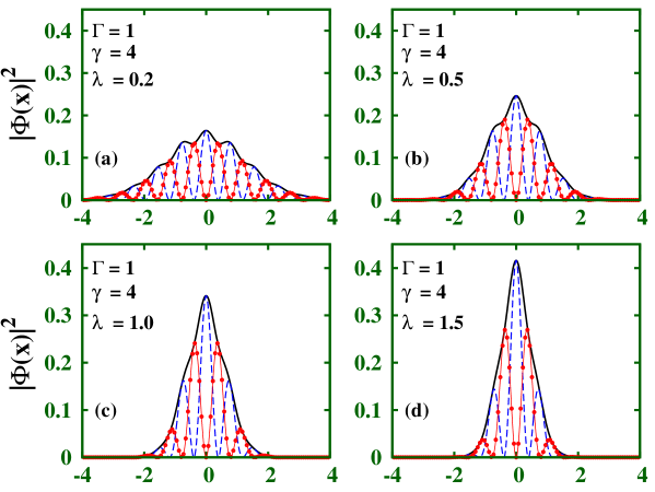
Figure 1: (Color online) Density profile of a self-attractive SO and Rabi coupled BEC under axial harmonic confinement $V(x)=\lambda^{2}x^{2}/2$. The nonlinearity strength is $gN=-0.8$. For panels (a)-(d), we set the Rabi coupling $\Gamma=1$, the SO coupling $\gamma=4$, and four values of the trap strength $\lambda$. For panels (e)-(h) we have $\Gamma=2$, $\gamma=3$, and the same values of $\lambda$ as in panels (a)-(d). The solid line depicts the density, while the dashed and point lines represent squared real and imaginary parts of the wave-function, respectively. Lengths are measured in units of the transverse confinement radius $a_{\perp}=\sqrt{\hbar/(m\omega_{\perp})}$.

We start the numerical analysis of the ground state structure in self-attractive BECs $(g<0)$ with SO and Rabi couplings in presence of a HO axial potential $V(x)=(\lambda^{2}/2)x^{2}$. In absence of the axial trapping potential $V(x)=0$, the existence of bright solitons as solutions of Eq. (11) is considered in [27, 30]. In [27] is shown that for $\gamma$ and $-gN$ constants, the increase of $\Gamma$ results in a compressed density profile with an increase of its height. On the other hand, by setting $\Gamma$ and $-gN$, the bright soliton is not subject to a significant compression, its height is reduced and the number of local maxima is increased with the increase of $\gamma$ [30]. In Fig. 1 we display the numerical results of a harmonically trapped self-attractive SO and Rabi coupled BEC. The density profile $|\Phi(x)|^{2}$, is plotted as a function of axial coordinate $x$. In panels (a)-(d), we set the strength of the nonlinearity $gN=-0.8$, the Rabi coupling $\Gamma=1$, the SO coupling $\gamma=4$, and four values of the strength of the trap $\lambda$. In panels (e)-(h), we set $\Gamma=2$, $\gamma=3$, and the same values of $gN$ and $\lambda$ as in panels (a)-(d). With the increase of the trap strength, the modulations of the squared of the real part and the imaginary one are subjected to a compression and their heights are increased. A noteworthy feature is a further increase of real part in comparison with the increase of the imaginary one. As a consequence of the effect caused by the trap strength the arrangement of the atoms in the condensate is restricted, their oscillations and its multi-peak nature decrease, thus giving rise to a shrunken condensate with a higher density. Reducing $\gamma$ and increasing $\Gamma$ at the same time, panels (a)-(e), (b)-(f), (c)-(g) and (d)-(h), our findings show the possibility of reduce the number of modulations and enlarge the density without a significant compression of the condensate. We compare the results of 1D NPSE (11) with those of the stationary 1D GPE obtained from (8) and both models match very good each other. The coincidence between these models can be understood since the 1D NPSE with $gN=-0.8$ becomes effectively 1D, i.e. the 1D NPSE becomes 1D GPE. However it is worth noting that, contrary to the cubic nonlinearity of 1D GPE, the nonpolynomial term of 1D NPSE is quite essential to predict the instability by collapse. This interesting phenomenon is present as long as the density of the condensate reaches the critical value $|\Phi|^{2}=(|g|N)^{-1}$ [27, 30]. The normalization constants obtained in Sec. 3 let us to get the same behaviors presented in [27, 30] but with a lower density. This density decrease gives rise to a greater variation of the parameters in particular in attractive SO and Rabi coupled BECs where the presence of instability by collapse is affected as shown below in the analysis of Fig. 5 (b).

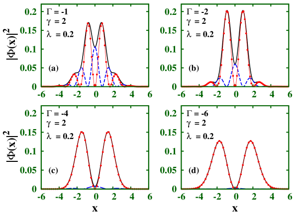
Figure 2: (Color online) Density profile of a self-attractive SO and Rabi coupled BEC under the axial harmonic confinement $V(x)=\lambda^{2}x^{2}/2$. Here, $gN=-0.8$, $\lambda=0.2$, $\gamma=2$ and four negative values of $\Gamma$. The solid line depicts the density, while the dashed and point lines represent squared real and imaginary parts of the wave-function, respectively. Lengths are measured in units of $a_{\perp}$.

Next we consider a harmonically trapped attractive condensate with a negative value of Rabi coupling. In Fig. 2 (a)-(d), we plot the density profile with the same nonlinearity as in Fig. 1, with a weak trap strength $\lambda=0.2$, the SO coupling $\gamma=2$ and four values of Rabi coupling $\Gamma$. Upon numerical simulation with the increase of $\Gamma(<0)$ the peaks of the density are diminished, the real component of the wave-function is suppressed Fig. 2 (d) and such a condensate is found to develop a notch in the central point $x=0$ between the two halves in a similar way as in the density distribution of a dark soliton. In Fig. 2 (b)-(c), the condensate seems to a grey-like soliton with the central notch having nonzero density. Using the same nonlinearity as in Fig. 1, setting the values of $\gamma$ and $\Gamma(<0)$, the increase of trap strength causes a compression of the condensate, its density becomes higher and the number of oscillations is reduced. All of this in a similar way as it was described in Fig. 1. About the symmetry of the system an interesting issue arises. As is predicted in [27], without the axial confinement and $\Gamma<0$, the real and imaginary parts of the wave-function are odd and even, respectively. In presence of the axial trapping potential and regardless of the sign of $\Gamma$ the real and imaginary parts of wave-function are even and odd, respectively.

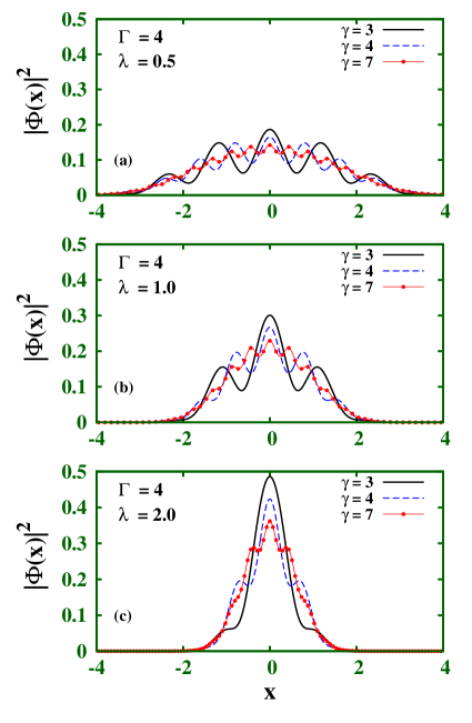
Figure 3: (Color online) Density profile of a harmonically trapped repulsive BEC with SO and Rabi couplings. We use the same form of the confinement as in Fig. 1, $gN=12$, $\Gamma=4$, $\gamma=3,4,7$ and three different values of $\lambda$, panels (a)-(c). Lengths are measured in units of $a_{\perp}$.

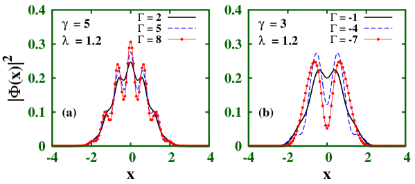
Figure 4: (Color online) Density profile of a harmonically trapped repulsive BEC with SO and Rabi couplings. We use $gN=16$ and the same form of the confinement as in Fig. 1 with $\lambda=1.2$. (a) $\gamma=5$ and $\Gamma=2,5,8$. (b) $\gamma=3$ and $\Gamma=-1,-4,-7$. Lengths are measured in units of $a_{\perp}$.

It is also relevant to analyze a self-repulsive $(g>0)$ BEC with SO and Rabi couplings. If $V(x)=0$ the atoms are spread out and the condensation is not possible. So a confinement potential is required to stabilize the condensate. Here we use a harmonic potential $V(x)=(\lambda^{2}/2)x^{2}$. In Fig. 3 (a)-(c), we plot the density $|\Phi(x)|^{2}$ as a function of axial coordinate $x$, with $gN=12$, $\Gamma=4$, $\gamma=3,4,7$ and three different values of $\lambda$. The increase of $\lambda$ generates the same effect on the total density as it was presented in Figs. 1 and 2. However for each of panels of Fig. 3, with constant values of $gN$, $\lambda$ and $\Gamma$, the interplay between the increase of SO coupling $\gamma$ and $\Gamma$ is reflected in two ways. The increase of $\gamma$ provides a linkage between the atoms of the two atomic hyperfine states, which in turn allows the increase of the multi-peak nature of the density. We also have a rearrangement of the atoms inside the trap, resulting in a less dense condensate and without its compression.

In Fig. 4 we plot the density of a trapped SO and Rabi coupled BEC with repulsive nonlinearity $gN=16$ $(g>0)$ and the strength of trap $\lambda=1.2$. In Fig. 4 (a), the increase of mixing between the two states accounting for $\Gamma$ leads to a rearrangement of the atoms without a significant change in the number of oscillations. While the real part increases the imaginary one undergoes a reduction without the appearance of new peaks in none of both contributions. So we have a density increase with an almost constant number of multi-peaks. Due to increase of $\Gamma(<0)$ for a constant value of $\gamma$ Fig. 4 (b), the condensate develops a notch in the central point and its seems to a dark-in-bright soliton with the central notch having nonzero density [29]. Our simulations show that the increase of $\lambda$ gives rise to a compressed and densest condensate as it has been presented in the above analysis of Figs. 1 and 2.

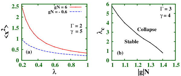
Figure 5: (Color online) (a) Root mean square (rms) size of the condensate $\langle x^{2}\rangle$ versus the trap strength $\lambda$. Here $\Gamma=2$, $\gamma=5$, and two values of the nonlinearity strength $gN$. (b) The critical trap strength $\lambda_{c}$ versus the attractive nonlinearity strength $|g|N$ with $\Gamma=3$ and $\gamma=4$. Lengths are measured in units of $a_{\perp}$.

The numerical results show that with the further increase of $\lambda$, the root mean square (rms) size of the condensate tends asymptotically to zero for both attractive $(g<0)$ and repulsive $(g>0)$ SO and Rabi coupled BECs. This trend is plotted in Fig. 5 (a). In the range $0\leq\lambda<0.2$ the attractive condensate remains. For $\lambda=0$ we have a bright SO and Rabi coupled BEC soliton. In the repulsive regime, the condensate is not present for $\lambda=0$, and its rms diverges as $\lambda\rightarrow 0$. In Fig. 5 (b), we present a numerical stability diagram for an attractive SO and Rabi coupled BEC with $\gamma=4$ and $\Gamma=3$. For an attractive interatomic interaction the condensate is stable for a critical maximum strength of interaction. When the strength of interaction increases beyond this critical value the condensate becomes unstable and it collapses. As usual, the experimental control of $g$ is achieved through manipulation of the s-wave scattering length $a$ using a Feshbach resonance. Of our numerical findings beyond the threshold $|g|N=1.4$ the instability by collapse occurs. On the other hand, for a fixed interatomic interaction and the manipulation of trap strength the SO and Rabi coupled BEC is stable for $\lambda<\lambda_{c}$. Even the condensate is stable in the range $0\leq\lambda<0.8$ provided that $|g|N\leq 1.4$. These results express the relevance of the effective nonpolynomial nonlinearity of Eq. (11) in the prediction of collapse. In [27] at fixed values of SO coupling $(\gamma=1)$ and Rabi coupling $(\Gamma=0.19)$, the collapse is predicted beyond $|g|N=1.2$. Here we show the possibility of increasing the threshold value of the collapse due to consideration of magnetization as a constraint in the calculation of the new normalization constants of Sec. 3. So the present study could be useful to give an idea of the maximum number of atoms in a stable SO and Rabi coupled BEC and could even be useful in planning future experiments.

The density patterns in this work for both attractive and repulsive BEC with SO and Rabi couplings in presence of harmonic traps are symmetric with respect to the $\gamma<0$ scenario. A possible verification of the results obtained in the present work perhaps it could be carried out taking into account the recent experimental realization of 2D SO coupling for BECs [42] and the experimental adjustment of $\Gamma$ and $\gamma$ carried out through of technique developed in [43]. Here is proposed a scheme for controlling SO coupling between two hyperfine ground states in a binary BEC through a fast and coherent modulation of the Raman laser intensities. Thus the experimental manipulation of the Raman coupling tunes the SO coupling.

5 Summary and outlook

In a bosonic quantum field theory we have derived an effective 1D system of two coupled NPHEs describing a harmonically confined dilute gas of bosonic atoms with nonlinear inter-atomic interactions, SO and Rabi couplings. The model takes into account both repulsive and attractive inter-atomic interactions. Provided that the many-body quantum state of the system is assumed to well-approximated by the Glauber coherent state, the 1D coupled NPHE becomes 1D coupled NPSE.

We focus on numerical analysis of the 1D coupled NPSE describing harmonically trapped attractive and repulsive SO and Rabi coupled BECs. The harmonic trap causes a strong reduction of the multi-peak nature of the condensate and it increases the density in both attractive and repulsive SO and Rabi coupled BECs. In the case of the repulsive interactions, the increase of $\gamma$ results in a less dense condensate without its compression and with a increase of the multi-peak nature of the density. On the other hand, the increase of $\Gamma$ leads to a density increase with an almost constant number of multi-peaks. Numerically we found a new structure of the SO and Rabi coupled BECs for both signs of the interaction and negative values of $\Gamma$. Here the condensate develops a notch in the central point and it seems to a dark-in-bright soliton with the central notch having nonzero density [29]. An interesting and significant result is the increment of the strength of the attractive nonlinearity at the collapse threshold due to the use of the magnetization as a constraint in the ground state calculation of the condensate under the combined action of the SO and Rabi couplings.

Extending the present analysis to another kind of potentials, such as the periodic potentials, one may expect interesting issues with non trivial effects. We also believe that our theoretical predictions could stimulate new experimental work in the SO and Rabi coupled BECs research. Another interesting question, such as the study of BECs with SO and Rabi couplings with higher pseudo-spin states in reduced dimensions, remain to be investigated in the future.

References

References

- [1] Lin Y-J, Jiménez-García K and Spielman I B 2011 Nature (London) 471, 83
- [2] Zhang J-Y, Ji S-C, Chen Z, Zhang L, Du Z-D, Yan B, Pan G-S, Zhao B, Deng Y-J, Zhai H, Chen S and Pan J-W 2012 Phys. Rev. Lett. 109, 115301
- [3] Wang P, Yu Z Q, Fu Z, Miao J, Huang L, Chai S, Zhai H and Zhang J 2012 Phys. Rev. Lett. 109, 095301 Cheuk L W, Sommer A T, Hadzibabic Z, Yefsah T, Bakr W S and Zwierlein M W 2012 Phys. Rev. Lett. 109, 095302
- [4] Manchon A, Koo H C, Nitta J, Frolov S M and Duine R A 2015 Nat. Mater. 14, 871 Tomka M, Pletyukhov M and Gritsev V 2015 Sci. Rep. 5, 13097 Hou Y-H and Yu Z 2015 Sci. Rep. 5, 15307
- [5] Zhai H 2012 Int. J. Mod. Phys. B 26, 1230001 Zheng W, Yu Z Q, Cui X and Zhai H 2013 J. Phys. B 46, 134007 Zhai H 2015 Rep. Prog. Phys. 78, (2), 026001
- [6] Xu Y, Zhang Y and Wu B 2013 Phys. Rev. A 87, 013614 Achilleos V, Frantzeskakis D J, Kevrekidis P G and Pelinovsky D E 2013 Phys. Rev. Lett. 110, 264101 Kartashov Y V, Konotop V V and Abdullaev F 2013 Phys. Rev. Lett. 111, 060402 Achilleos V, Stockhofe J, Kevrekidis P G, Frantzeskakis D J and Schmelcher P 2013 Eur. Phys. Lett. 103, 20002 Cao S, Shan C-J, Zhang D-W, Qin X and Xu J 2015 J. Opt. Soc. Am. B 32, 201
- [7] Sakaguchi H, Li B and Malomed B A 2014 Phys. Rev. E 89, 032920 Lobanov V E, Kartashov Y V and Konotop V V 2014 Phys. Rev. Lett. 112, 180403 Mardonov Sh, Sherman E Ya, Muga J G, Wang H-W, Ban Y and Chen X 2015 Phys. Rev. A 91, 043604
- [8] Stanescu T D, Anderson B and Galitski V 2008 Phys. Rev. A 78, 023616 Ho T L and Zhang S 2011 Phys. Rev. Lett. 107, 150403 Xu X-Q and Han J H 2011 Phys. Rev. Lett. 107, 200401 Radic J, Sedrakyan T A, Spielman I B and Galitski V 2011 Phys. Rev. A 84, 063604 Zhou X F, Zhou J and Wu C 2011 Phys. Rev. A 84, 063624 Ruokokoski E, Huhtamäki J A M and Möttönen M 2012 Phys. Rev. A 86, 051607(R) Sakaguchi H and Li B 2013 Phys. Rev. A 87, 015602 Fetter A L 2014 Phys. Rev. A 89, 023629 Fetter A L 2015 J. Low Temp. Phys. 180, 37 Ramachandhran B, Opanchuk B, Liu X-J, Pu H, Drummond P D and Hu H 2012 Phys. Rev. A 85, 023606 Sakaguchi H, Sherman E Ya and Malomed B A 2016 Phys. Rev. E 94, 032202
- [9] Li Y, Pitaevskii L P and Stringari S 2012 Phys. Rev. Lett. 108, 225301
- [10] Barnett R, Powell S, Grass T, Lewenstein M and Das Sarma S 2012 Phys. Rev. A 85, 023615
- [11] He P-S 2013 Eur. Phys. J. D 67 48 He P-S, You W-L and Liu W-M 2013 Phys. Rev. A 87, 063603
- [12] Cheng Y S, Tang G H and Adhikari S K 2014 Phys. Rev. A 89, 063602
- [13] Zezyulin D A, Driben R, Konotop V V and Malomed B A 2013 Phys. Rev. A 88, 013607
- [14] Zhang D-W, Fu L-B, Wang Z D and Zhu S-L 2012 Phys. Rev. A 85, 043609 Garcia-March M-A, Mazzarella G, Dell’Anna L, Juliá-Díaz B, Salasnich L and Polls A 2014 Phys. Rev. A 89, 063607 Gallemí A, Guilleumas M, Mayol R and Mateo A-M 2016 Phys. Rev. A 93, 033618
- [15] Liao R, Huang Z-G, Lin X-M and Fialko O 2014 Phys. Rev. A 89, 063614 Ji S-C, Zhang J-Y, Zhang L, Du Z-D, Zheng W, Deng Y-J, Zhai H, Chen S and Pan J-W 2014 Nature Physics 10, 314
- [16] Sinha S, Nath R and Santos L 2011 Phys. Rev. Lett. 107, 270401
- [17] Wang C, Gao C, Jian C M and Zhai H 2010 Phys. Rev. Lett. 105, 160403
- [18] Hu H, Ramachandhran B, Pu H and Liu X-J 2012 Phys. Rev. Lett. 108, 010402
- [19] Ozawa T and Baym G 2012 Phys. Rev. A 85, 063623
- [20] Zhu C, Dong L and Pu H 2016 J. Phys. B 49, 145301
- [21] Hu F-Q, Wang J-J, Yu Z-F, Zhang A-X and Xue J-K 2016 Phys. Rev. E 93, 022214
- [22] Bhat I A, Mithun T, Malomed B A and Porsezian K 2015 Phys. Rev. A 92, 063606 Bhuvaneswari S, Nithyanandan K, Muruganandam P and Porsezian K 2016 J. Phys. B 49, 245301
- [23] Deng Y, Cheng J, Jing H, Sun C-P and Yi S 2012 Phys. Rev. Lett. 108, 125301 Xu Y, Zhang Y and Zhang C 2015 Phys. Rev. A 92, 013633 Jiang X, Fan Z, Chen Z, Pang W, Li Y and Malomed B A 2016 Phys. Rev. A 93, 023633 Li T, Yi S and Zhang Y 2016 Phys. Rev. A 93, 053602 Kato M, Zhang X-F, Sasaki D and Saito H 2016 Phys. Rev. A 94, 043633
- [24] Dalfovo F, Giorgini S, Pitaevskii L P and Stringari S 1999 Rev. Mod. Phys. 71, 463
- [25] Cornish S L, Thompson S T and Wieman C E 2006 Phys. Rev. Lett. 96, 170401 Eiermann B, Anker Th, Albiez M, Taglieber M, Treutlein P, Marzlin K-P and Oberthaler M-K 2004 Phys. Rev. Lett. 92, 230401 Giamarchi T 2004 Quantum Physics in One Dimension (Oxford University Press) Cazalilla M A, Citro R, Giamarchi T, Orignac E and Rigol M 2011 Rev. Mod Phys. 83, 1405
- [26] Salasnich L, Parola A and Reatto L 2002 Phys. Rev. A 65, 043614 Sinha S and Santos L 2007 Phys. Rev. Lett. 99, 140406 Muñoz Mateo A and Delgado V 2008 Phys. Rev. A 77, 013617 Muruganandam P and Adhikari S K 2012 Laser Phys. 22, 813–820 Chiquillo E 2014 Laser Phys. 24, 085502
- [27] Salasnich L and Malomed B A 2013 Phys. Rev. A 87, 063625
- [28] Salasnich L, Cardoso W B and Malomed B A 2014 Phys. Rev. A 90, 033629
- [29] Adhikari S K 2014 Phys. Rev. A 89, 043615 Becker C, Stellmer S, Soltan-Panahi1 P, Dörscher S, Baumert M, Richter E-M, Kronjäger J, Bongs K and Sengstock K 2008 Nature Physics 4, 496 Nistazakis H E, Frantzeskakis D J, Kevrekidis P G, Malomed B A and Carretero-González R 2008 Phys. Rev. A 77, 033612
- [30] Chiquillo E 2015 J. Phys. A 48, 475001
- [31] Barbiero L and Salasnich L 2014 Phys. Rev. A 89, 063605
- [32] Salasnich L 2015 Quodons in Mica Discrete Bright Solitons in Bose-Einstein Condensates and Dimensional Reduction in Quantum Field Theory (Springer Series in Materials Science) ed JFR Archilla, N Jiménez, V J Sánchez-Morcillo and L M García (Berlin: Springer) Vol 221
- [33] Salasnich L 2014 A modern introduction to photons, atoms and many-body systems Quantum Physics of Light and Matter (Cham: Springer) p 167
- [34] Rogel-Salazar J, Choi S, New G H C and Burnett K 2004 J. Opt. B: Quantum Semiclass. Opt. 6 33-59
- [35] Stoof H T C, Gubbels K and Dickerscheid D 2009 Ultracold Quantum Fields (Berlin: Springer) p 131
- [36] Glauber R 1963 Phys. Rev. 131, 2766 Zhang W-M, Feng D H and Gilmore R 1990 Rev. Mod. Phys. 62, 867
- [37] Muruganandam P and Adhikari S K 2009 Comput. Phys. Commun. 180, 1888
- [38] Bao W and Cai Y 2011 East Asia Journal on Applied Mathematics 1, 49 Lim F-Y and Bao W 2008 Phys. Rev. E 78, 066704 Bao W and Lim F-Y 2008 Siam J. Sci. Comp. 30, 1925
- [39] Gautam S and Adhikari S K 2014 Phys. Rev. A 90, 043619 Gautam S and Adhikari S K 2015 Laser Phys. Lett. 12, 045501
- [40] Gautam S and Adhikari S K 2015 Phys. Rev. A 91, 013624 Gautam S and Adhikari S K 2015 Phys. Rev. A 91, 063617
- [41] Jiang W, Wang H and Li X 2013 Comput. Phys. Commun. 184, 2396
- [42] Wu Z, Zhang L, Sun W, Xu X-T, Wang B-Z, Ji S-C, Deng Y, Chen S, Liu X-J, Pan J-W 2016 Science 354, 83
- [43] Zhang Y, Chen G and Zhang C 2013 Sci. Rep. 3, 1937 Lian J, Yu L, Liang J-Q, Chen G and Jia S 2013 Sci. Rep. 3, 3166 Jiménez-García K, LeBlanc L J, Williams R A, Beeler M C, Qu C, Gong M, Zhang C and Spielman I B 2015 Phys. Rev. Lett. 114, 125301