Radio haloes in nearby galaxies modelled with 1D cosmic-ray transport using SPINNAKER

Abstract

We present radio continuum maps of 12 nearby ($D\leq 27$ Mpc), edge-on ($i\geq 76\degr$), late-type spiral galaxies mostly at $1.4$ and 5 GHz, observed with the Australia Telescope Compact Array, Very Large Array, Westerbork Synthesis Radio Telescope, Effelsberg 100-m and Parkes 64-m telescopes. All galaxies show clear evidence of radio haloes, including the first detection in the Magellanic-type galaxy NGC 55. In 11 galaxies, we find a thin and a thick disc that can be better fitted by exponential rather than Gaussian functions. We fit our SPINNAKER (SPectral INdex Numerical Analysis of K(c)osmic-ray Electron Radio-emission) 1D cosmic-ray transport models to the vertical model profiles of the non-thermal intensity and to the non-thermal radio spectral index in the halo. We simultaneously fit for the advection speed (or diffusion coefficient) and magnetic field scale height. In the thick disc, the magnetic field scale heights range from 2 to 8 kpc with an average across the sample of $3.0\pm 1.7$ kpc; they show no correlation with either star-formation rate (SFR), SFR surface density ($\Sigma_{\rm SFR}$) or rotation speed ($V_{\rm rot}$). The advection speeds range from 100 to 700 $\rm km\,s^{-1}$ and display correlations of $V\propto\rm SFR^{0.36\pm 0.06}$ and $V\propto\Sigma_{\rm SFR}^{0.39\pm 0.09}$; they agree remarkably well with the escape velocities ($0.5\leq V/V_{\rm esc}\leq 2$), which can be explained by cosmic-ray driven winds. Radio haloes show the presence of disc winds in galaxies with $\Sigma_{\rm SFR}>10^{-3}~{}\rm M_{\sun}\,yr^{-1}\,kpc^{-2}$ that extend over several kpc and are driven by processes related to the distributed star formation in the disc.

1 Introduction

This paper is a follow-up study of our recent paper about the ‘Advective and diffusive cosmic-ray transport in galactic haloes’ (Heesen et al., 2016, hereafter HD16), where we presented 1D cosmic ray transport models now implemented in the software SPINNAKER (SPectral INdex Numerical Analysis of K(c)osmic-ray Electron Radio-emission). We have extended our previous radio continuum observations of two edge-on galaxies, adding another 10 galaxies, to study advection speed, magnetic field scale height and diffusion coefficient across a wider range of galactic parameters. We then study the influence of the star-formation rate (SFR), SFR surface density ($\Sigma_{\rm SFR}$) and rotation speed ($V_{\rm rot}$) on these results. We use a combination of so far unpublished and archival data from the Australia Telescope Compact Array (ATCA), the Very Large Array (VLA) and the Westerbork Synthesis Radio Telescope (WSRT). For a sub-sample of four galaxies we use single-dish observations with both the Effelsberg 100-m and Parkes 64-m telescopes in order to complement the interferometric data. The majority of the interferometric observations were taken before the recent upgrade of the correlators, so that we mostly use 100-MHz-bandwidths, rather than the GHz-bandwidths which are available nowadays. While this leads to reduced sensitivities of tens rather than a few $\mu\rm Jy\,beam^{-1}$, a sample like this is a good reference against which to compare the new wide-band data as observed with the Karl G. Jansky VLA (Wiegert et al., 2015).

Our sample contains 12 nearby edge-on galaxies (11 late-type spiral galaxies and 1 Magellanic-type galaxy), which lie in the SFR range of $0.1\leq{\rm SFR/(M_{\sun}\,yr^{-1})}\leq 16$. Where possible, we produce maps that have a spatial resolution of 1 kpc or better. The reason for this is to allow the separation of the thin and thick radio disc, which are present in most galaxies. The thin disc (with a scale height of a few 100 pc) represents a region of current/recent star formation populated by supernova remnants and H ii regions (Ferrière, 2001); the thick disc (with a scale height of a few kpc) is what we refer to in this work as the ‘halo’ and represents the region of extra-planar gas, magnetic fields and cosmic rays with no ongoing star formation (Rossa & Dettmar, 2003a; Krause et al., 2017). As we will show in this paper, we observe a transition between thin and thick disc at a height of $|z|\approx 1~{}\rm kpc$, so that we will refer to the halo as emission at $|z|\gtrapprox 1$ kpc. We are aware that the transition between the disc and halo is gradual (the ‘disc–halo’ interface), and the observed transition will also depend on the spatial resolution.

Table 1: General properties of our sample galaxies.

Galaxy	$i^{\rm a}$	$d_{25}^{\rm b}$	$D^{\rm c}$	$M_{B}^{\rm d}$	$\rm Type^{e}$	$\rm Nucleus^{f}$	$\rm SFR^{g}$	$r_{\star}^{\rm h}$	$\log_{10}(\Sigma_{\rm SFR})^{\rm i}$	$\log_{10}(M_{\rm tot})^{\rm j}$	$V_{\rm rot}^{\rm k}$
	($\degr$)	($\arcmin$)	(Mpc)	(mag)			($\rm M_{\sun}\,yr^{-1}$)	(kpc)	($\rm M_{\sun}\,yr^{-1}\,kpc^{-2}$)	($\rm M_{\sun}$)	($\rm km\,s^{-1}$)
NGC 55	$80.0$	$34.1$	$1.9$	$-18.89$	SBm		$0.16$	$6.2$	$-2.87$	$10.26$	$91$
NGC 253	$78.5$	$25.8$	$3.9$	$-20.64$	SABc	H ii	$6.98$	$11.8$	$-1.80$	$11.16$	$205$
NGC 891	$89.0$	$12.2$	$10.2$	$-20.09$	Sb	H ii	$4.72$	$11.7$	$-1.96$	$11.28$	$212$
NGC 3044	$90.0$	$4.4$	$18.7$	$-19.53$	SBc		$2.03$	$9.8$	$-2.17$	$10.81$	$153$
NGC 3079	$88.0$	$7.7$	$19.7$	$-20.94$	SBcd	Sy2	$9.09$	$13.3$	$-1.79$	$11.35$	$208$
NGC 3628	$87.0$	$14.8$	$7.9$	$-20.01$	Sb	T2	$1.73$	$10.7$	$-2.32$	$11.26$	$215$
NGC 4565	$90.0$	$16.2$	$24.7$	$-22.37$	Sbc	Sy$1.9$	$5.69$	$37.1$	$-2.88$	$11.91$	$244$
NGC 4631	$85.0$	$14.7$	$6.9$	$-20.12$	SBcd	H ii	$2.89$	$12.1$	$-2.20$	$10.82$	$138$
NGC 4666	$76.0$	$4.2$	$26.6$	$-21.14$	SABc	LINER	$16.19$	$14.0$	$-1.58$	$11.15$	$193$
NGC 5775	$84.0$	$3.9$	$26.9$	$-20.71$	Sbc	H ii	$9.98$	$14.4$	$-1.81$	$11.09$	$187$
NGC 7090	$89.0$	$6.8$	$10.6$	$-19.70$	Sc		$0.62$	$7.2$	$-2.41$	$10.57$	$124$
NGC 7462	$90.0$	$5.0$	$13.6$	$-18.57$	SBbc		$0.28$	$7.5$	$-2.80$	$10.46$	$112$

Most of our sample galaxies have been studied in the radio (continuum and line) in detail before, so we will give here only a brief summary of their most notable properties (general properties are summarized in Table 1). NGC 55, a Magellanic-type (irregular, of intermediate mass between dwarf and spiral galaxies) galaxy and member of the Sculptor group has a very thick H i disc extending up to a height of 10 kpc into the halo (Westmeier et al., 2013). Thick H i discs could be a sign of a galactic fountain or on-going gas accretion. NGC 253, another member of the Sculptor group, is a prototypical nuclear starburst galaxy and is most notable for its ‘dumbbell shaped’ radio halo caused by strong synchrotron cooling in the centre of the galaxy (Heesen et al., 2009a, b, 2011). This galaxy is also notable for a very bright X-ray halo, which shows the presence of a ‘disc wind’, which is unrelated to the nuclear outflow (Bauer et al., 2008). The distinction between nuclear outflows and disc winds is important for this study: nuclear outflows emanate from the central few 100 pc driven by a combination of concentrated star formation and jets from active galactic nuclei (AGNs). In our work, we concentrate on the disc winds, which extend over a large fraction of the star-forming disc over several kpc at least, although the scale can be smaller than 10-kpc (see Westmoquette et al., 2011, for a discussion of nuclear outflows vs. disc winds).

NGC 891 has a prominent thick H i disc, the kinematics of which have been studied in detail by Oosterloo et al. (2007). They showed that this galaxy still accretes intergalactic matter, so that the halo is only in part caused by the galactic fountain. NGC 891 is the best case to study the influence of on-going accretion on to a radio halo. NGC 3044 hosts a large H i supershell that extends to a height of 3 kpc above the midplane (Lee & Irwin, 1997). These H i supershells require dozens of supernovae (SNe) and are essential for an active disc–halo interface. We expect these kind of features to be abundant in our galaxies, but the spatial resolution of our observations is not high enough to resolve these features.

NGC 3079 is a case in point for a galaxy with a nuclear outflow driven by a combination of starburst and low-luminosity AGN. Jets from the AGN entrain the surrounding material which is subsequently transported away from the nucleus (Middelberg et al., 2007; Shafi et al., 2015). Above and below the nucleus, there are well-defined kpc-sized lobes of non-thermal emission, surrounded by filamentary H $\alpha$ emission that have counterparts in X-ray emission (Cecil et al., 2001, 2002). While the filamentary emission is clearly connected to the nuclear outflow and AGN-driven jets, there are also indications for a disc wind in this galaxy. First, there are vertical H $\alpha$ and dust filaments extending over the full extent of the disc (Cecil et al., 2001), reminiscent of a ‘boiling disc’ in NGC 253 (Sofue et al., 1994), which is indicative of an active disc–halo interface. Second, the X-ray emission in the halo extends, as in NGC 253, for several kpc away from the nuclear outflow (Strickland et al., 2004); it is questionable that the two are related. In order to study the disc wind only, we have masked the radio continuum emission stemming from the nuclear outflow in the following analysis.

NGC 3628, a nuclear starburst galaxy, is a member of the Leo Triplet and possesses a 140-kpc long tidal tail of atomic hydrogen detected in the 21-cm H i line (Haynes et al., 1979). NGC 4565 has a ‘lagging’ H i halo, where the rotational velocity of the neutral gas decreases with increasing distance from the midplane. This makes it likely that this galaxy has an on-going galactic fountain, in spite of the galaxy having only little extra-planar H i emission (Zschaechner et al., 2012). NGC 4631 is the galaxy with arguably the most prominent radio halo. This is in part caused by gravitational interaction with its neighbour NGC 4656, where a ’spur’ of ordered magnetic fields leads to the neighbour galaxy (Hummel et al., 1988; Mora & Krause, 2013). This merger has probably caused a starburst in the past that led to an outflow the result of which we see now (Irwin et al., 2011). NGC 4666 is a starburst galaxy with outflowing ionized H $\alpha$ emission (Dahlem et al., 1997; Voigtländer et al., 2013), while NGC 5775 is the prototypical X-shaped halo magnetic field galaxy (Tüllmann et al., 2000; Soida et al., 2011). These galaxies have magnetic field structures that look in projection like an ‘X’. The field shapes are thought to be caused by either a galactic dynamo in the halo or by the interaction of the magnetic field lines with a galactic wind (Heesen et al., 2009b). Finally, NGC 7090 and NGC 7462 are rather unremarkable galaxies although both possess a layer of extra-planar H $\alpha$ and H i emission (Rossa & Dettmar, 2003a, b; Dahlem et al., 2005).

In this paper, we present observations at $L$, $C$ and $X$ band ($1.4$, 5 and $8.5$ GHz) in order to study vertical profiles of the non-thermal intensities and the non-thermal radio spectral index. We use exponential and Gaussian functions to model the vertical profiles of the non-thermal radio emission. These profiles are then fitted with our cosmic-ray transport models, in order to measure advection speeds, diffusion coefficients and magnetic field scale heights. We estimate magnetic field strengths from energy equipartition (Beck & Krause, 2005) and use the total infrared luminosity to determine photon energy densities. Thus, we can take both the synchrotron and inverse Compton (IC) losses of the CR electrons (CREs) into account.

This paper is organized as follows: in Section 2 we describe our observations and data reduction techniques. In Section 3, we motivate and present our cosmic-ray transport models. Results are presented in Section 4, followed by the discussion in Section 5. We finish off with our conclusions in Section 6. Figure 2 shows the radio continuum maps for NGC 4631, followed by Figs 3 and 4, which contain a step-by-step guide on how we obtained the best-fitting cosmic-ray transport model for this particular galaxy. Figure 5 summarizes the results for our sample with an atlas of maps and models presented in Appendix D. Throughout the paper, the radio spectral index $\alpha$ is defined in the sense $S_{\nu}\propto\nu^{\alpha}$ and quantities averaged across the sample are error m and presented with an uncertainty of $\pm 1\sigma$.

2 Observations and data reduction

Table 2: Observation details for the galaxies presented in this paper.

Galaxy	Banda	$\nu^{\rm b}$	$\rm Telescope^{\rm c}$	$\rm Configuration^{\rm d}$	$\rm Project^{\rm e}$	$\rm Time^{\rm f}$	$\rm Date^{\rm g}$	$\rm Notes^{h}$	$\rm Reference^{\rm i}$
		(GHz)				(h)
NGC 55	$L$	$1.37$	ATCA	750D	C287	$8.7$	1993 Aug 1	Mosaic	17
$\ldots$	$\ldots$	$\ldots$	$\ldots$	375	C287	$11.2$	1995 Jan 12	$\ldots$	$\ldots$
$\ldots$	$\ldots$	$\ldots$	$\ldots$	750A	C287	$11.1$	1995 Oct 25	$\ldots$	$\ldots$
$\ldots$	$\ldots$	$\ldots$	$\ldots$	H75	C1341	$5.0$	2005 Jul 17	Mosaic	This work
$\ldots$	$\ldots$	$\ldots$	$\ldots$	EW352	C1341	$9.4$	2005 Oct 7	$\ldots$	$\ldots$
$\ldots$	$C$	$4.80$	$\ldots$	375	C287	$3.6$	1994 Mar 29	Mosaic	17
$\ldots$	$\ldots$	$\ldots$	$\ldots$	375	C287	$10.2$	1994 Mar 30	$\ldots$	$\ldots$
$\ldots$	$\ldots$	$\ldots$	$\ldots$	375	C287	$7.8$	1994 Mar 31	$\ldots$	$\ldots$
$\ldots$	$\ldots$	$\ldots$	$\ldots$	375	C287	$12.5$	1994 Nov 23	$\ldots$	$\ldots$
$\ldots$	$\ldots$	$\ldots$	$\ldots$	750A	C287	$5.1$	1995 Mar 1	$\ldots$	$\ldots$
$\ldots$	$\ldots$	$\ldots$	$\ldots$	375	C287	$5.3$	1995 Aug 16	$\ldots$	$\ldots$
$\ldots$	$\ldots$	$\ldots$	$\ldots$	375	C287	$10.2$	1995 Nov 24	$\ldots$	$\ldots$
$\ldots$	$\ldots$	$4.67$	$\ldots$	EW352	C1974	$7.6$	2008 Nov 22	$\ldots$	This work
$\ldots$	$\ldots$	$\ldots$	$\ldots$	EW364	C1974	$9.9$	2009 Feb 13	$\ldots$	$\ldots$
$\ldots$	$C$	$5.60$	$\ldots$	H168	C1974	$7.6$	2010 Mar 27	$\ldots$	$\ldots$
$\ldots$	$C$	$4.80$	Parkes	single-dish	P697	$16.0$	2010 Oct 7	Merged	$\ldots$
NGC 253	$L$	$1.46$	VLA	B+C+D	AC278	$4.1$	1990 Sep–1991 Mar	Mosaic	2
$\ldots$	$C$	$4.86$	$\ldots$	D	AH844	$35.8$	2004 Jul 4–24	Mosaic	10
$\ldots$	$\ldots$	$4.85$	Effelsberg	single-dish	N/A	N/A	1997	Merged	$\ldots$
NGC 891	$L$	$1.39$	WSRT	Multiple	R02B	240	2002 Aug–Dec		13
$\ldots$	$C$	$4.86$	VLA	D	AA94	$11.2$	1988 Aug 29		16
$\ldots$	$\ldots$	$4.85$	Effelsberg	single-dish	44–95	$9.1$	1996 Feb–Aug		6
NGC 3044	$L$	$1.49$	VLA	B	AI28	$3.1$	1986 Aug 1		This work
$\ldots$	$\ldots$	$\ldots$	$\ldots$	C	AI23	$0.8$	1985 Jul 25		11
$\ldots$	$\ldots$	$\ldots$	$\ldots$	D	AI31	$1.1$	1987 Apr 28/30		$\ldots$
$\ldots$	$C$	$4.86$	$\ldots$	C	AB676	$0.8$	1993 Jun 13		4
$\ldots$	$\ldots$	$\ldots$	$\ldots$	D	AM573	$1.1$	1997 Nov 6		This work
$\ldots$	$\ldots$	$\ldots$	$\ldots$	D	AI31	$1.0$	1987 Apr 28		11
NGC 3079	$L$	$1.66$	VLA	B	BS44	$1.0$	1997 Mar 8		This work
$\ldots$	$\ldots$	$1.41$	$\ldots$	CD	BS44	$2.4$	1997 Oct 2		$\ldots$
$\ldots$	$\ldots$	$1.43$	$\ldots$	C	AB740	$1.3$	1996 Feb 17		$\ldots$
$\ldots$	$C$	$4.71$	$\ldots$	C	AC277	$3.9$	1990 Dec 9		3
$\ldots$	$\ldots$	$4.86$	$\ldots$	D	AD177	$2.5$	1986 Jan 16		This work
NGC 3628	$L$	$1.49$	VLA	CD	AS300	$4.3$	1988 Mar 25		14
$\ldots$	$\ldots$	$\ldots$	$\ldots$	D	AS300	$8.4$	1987 Apr 7		$\ldots$
$\ldots$	$C$	$4.86$	$\ldots$	D	AK243	$7.7$	1991 Mar 28		7
NGC 4565	$L$	$1.49$	VLA	B	AS326	$3.8$	1988 Jan 29		16
$\ldots$	$\dots$	$1.48$	$\ldots$	D	AS326	$10.6$	1988 Aug 28		$\ldots$
$\ldots$	$C$	$4.86$	$\ldots$	D	AK424	$3.4$	1996 Sep 28		6
NGC 4631	$L$	$1.37$	WSRT	maxi-short	N/A	$6.0$	2003 Apr 3		1
$\ldots$	$C$	$4.86$	VLA	D	AH369	$12.1$	1989 Nov 22/26	Mosaic	9
$\ldots$	$\ldots$	$\ldots$	$\ldots$	D	AD896	$4.3$	1999 Apr 14	Mosaic	12
$\ldots$	$\ldots$	$4.85$	Effelsberg	single-dish	55–94	$6.3$	1996 Feb–Aug	Merged	6
NGC 4666	$L$	$1.43$	VLA	CD	AD346	$3.5$	1994 Nov 20		5
$\ldots$	$\ldots$	$1.49$	$\ldots$	D	AS199	$0.2$	1984 Aug 31		This work
$\ldots$	$C$	$4.86$	$\ldots$	D	AD326	$12.5$	1993 Dec 20/24		5
NGC 5775	$L$	$1.49$	VLA	B	AI0028	$3.2$	1986 Aug 1		8
$\ldots$	$\ldots$	$1.48$	$\ldots$	B	AB492	$1.2$	1989 Aug 4		$\ldots$
$\ldots$	$\ldots$	$1.49$	$\ldots$	C	AH368	$3.6$	1990 Nov 19/24		$\ldots$
$\ldots$	$\ldots$	$\ldots$	$\ldots$	D	AI31	$1.9$	1987 Apr 27/30		11
$\ldots$	$X$	$8.45$	$\ldots$	D	AD455	$13.4$	2001 Dec 14		15

2.1 Radio continuum maps

We used a variety of radio continuum observations, most of them already published, which we obtained from the respective telescope archives. We re-reduced these data, which we describe in the following. In Table 2, we present a summary of the observations used, including references where the data were published first.

2.1.1 Australia Telescope Compact Array

Observations of NGC 55 with the ATCA were calibrated following standard procedures with MIRIAD (Sault, Teuben & Wright, 1995), where we set the flux density of the primary calibrator J1938$-$634 with MFCAL (part of MIRIAD). At $L$ band we combined previously published data from Wells (1997) with newly obtained data as part of the Local Volume H i Survey (LVHIS). At $C$ band, we used again the previously published data of Wells (1997) and added new observations; these data were observed in 2008 November and 2009 February in the radio continuum mode with a bandwidth of 256 MHz, split into two IFs of 128 MHz bandwidth each. More data were observed in 2010 with the upgraded Compact Array Broad-band Backend (CABB; Wilson et al., 2011) receiver ($4.7$–$6.6$ GHz). Because NGC 55 has an angular extension that exceeds the primary beam both at $L$ and $C$ band, we used several pointings to mosaic the galaxy. The calibrated $(u,v)$ data were precessed to J$2000.0$ if necessary and exported into the FITS format. The observations and data reduction of NGC 7090 and 7462 were already presented in HD16.

2.1.2 Very Large Array

Observations with the VLA were calibrated following standard procedures with AIPS. We set the flux density of the primary calibrator (either 3C 48 or 286) according to the model by Baars et al. (1977). Since the data were observed only with the ‘historical’ VLA prior to the upgrade of the correlator, observations had bandwidths of 100 MHz split into two IFs of 50 MHz each. We used data at $L$ band (NGC 253, 3044, 3079, 3628, 4565, 4666 and 5775), $C$ band (NGC 253, 891, 3044, 3079, 3628, 4565, 4631 and 4666) and $X$ band (NGC 5775). We used maps of NGC 253 published earlier without either re-calibrating or re-imaging of the data. The observations at $L$ and $C$ band were already described in Carilli et al. (1992) and Heesen et al. (2009a), respectively. The calibrated data were precessed to J$2000.0$ where necessary and exported into the FITS format.

2.1.3 Westerbork Synthesis Radio Telescope

We used a $1.4$-GHz map of NGC 891 observed with the WSRT, which was already presented by Oosterloo et al. (2007). Furthermore, we used the $1.4$-GHz map of NGC 4631 again observed with the WSRT. This galaxy was observed as part of the WSRT SINGS survey (Braun et al., 2007) and we re-imaged the map as described below.

Table 3: Radio properties of our sample galaxies.

Galaxy	$\Theta_{\rm FWHM}^{\rm a}$	$\nu_{1}^{\rm b}$	$\nu_{2}^{\rm b}$	$S_{1}^{\rm c}$	$S_{\rm 1,nt}^{\rm d}$	$S_{2}^{\rm c}$	$S_{\rm 2,nt}^{\rm d}$	$\alpha^{\rm e}$	$\alpha_{\rm nt}^{\rm f}$
	(arcsec)	(GHz)		(Jy)	(Jy)	(Jy)	(Jy)
NGC 55	$41.10$	$1.36$	$5.56$	$0.6082\pm 0.0172$	$0.5219\pm 0.0152$	$0.2966\pm 0.0107$	$0.2216\pm 0.0084$	$-0.51\pm 0.03$	$-0.61\pm 0.03$
NGC 253	$30.00$	$1.46$	$4.85$	$6.3000\pm 0.1409$	$6.2133\pm 0.1390$	$2.7100\pm 0.0678$	$2.6331\pm 0.0659$	$-0.70\pm 0.03$	$-0.72\pm 0.03$
NGC 891	$17.30$	$1.39$	$4.86$	$0.7720\pm 0.0155$	$0.7663\pm 0.0154$	$0.2720\pm 0.0056$	$0.2670\pm 0.0056$	$-0.83\pm 0.02$	$-0.84\pm 0.02$
NGC 3044	$7.80$	$1.49$	$4.86$	$0.1040\pm 0.0021$	$0.0990\pm 0.0020$	$0.0450\pm 0.0009$	$0.0406\pm 0.0009$	$-0.71\pm 0.02$	$-0.75\pm 0.03$
NGC 3079	$8.30$	$1.53$	$4.71$	$0.8360\pm 0.0169$	$0.8262\pm 0.0167$	$0.3430\pm 0.0350$	$0.3342\pm 0.0341$	$-0.79\pm 0.09$	$-0.80\pm 0.09$
NGC 3628	$17.70$	$1.49$	$4.86$	$0.5482\pm 0.0198$	$0.5433\pm 0.0196$	$0.2287\pm 0.0051$	$0.2243\pm 0.0050$	$-0.74\pm 0.04$	$-0.75\pm 0.04$
NGC 4565	$13.10$	$1.49$	$4.86$	$0.1599\pm 0.0116$	$0.1585\pm 0.0115$	$0.0557\pm 0.0012$	$0.0544\pm 0.0013$	$-0.89\pm 0.06$	$-0.90\pm 0.06$
NGC 4631	$23.10$	$1.37$	$4.86$	$1.2850\pm 0.0287$	$1.2451\pm 0.0283$	$0.4654\pm 0.0251$	$0.4303\pm 0.0236$	$-0.80\pm 0.05$	$-0.84\pm 0.05$
NGC 4666	$15.70$	$1.45$	$4.86$	$0.3870\pm 0.0087$	$0.3712\pm 0.0083$	$0.1370\pm 0.0039$	$0.1230\pm 0.0035$	$-0.86\pm 0.03$	$-0.91\pm 0.03$
NGC 5775	$8.25$	$1.49$	$8.46$	$0.2680\pm 0.0097$	$0.2630\pm 0.0095$	$0.0598\pm 0.0022$	$0.0556\pm 0.0020$	$-0.86\pm 0.03$	$-0.89\pm 0.03$
NGC 7090	$13.80$	$1.38$	$4.67$	$0.0563\pm 0.0030$	$0.0519\pm 0.0029$	$0.0153\pm 0.0023$	$0.0114\pm 0.0018$	$-1.07\pm 0.13$	$-1.24\pm 0.14$
NGC 7462	$13.90$	$1.38$	$4.67$	$0.0256\pm 0.0009$	$0.0238\pm 0.0012$	$0.0066\pm 0.0002$	$0.0050\pm 0.0006$	$-1.10\pm 0.04$	$-1.27\pm 0.11$

Table 4: Further radio properties of our sample galaxies.

Galaxy	$d_{\rm maj}^{\rm a}$	$d_{\rm min}^{\rm a}$	$\rm PA^{b}$	$\sigma_{1}^{\rm c}$	$\sigma_{2}^{\rm c}$	$W_{\rm stripe}$d	$W_{\rm stripe}$d	Stripe centree
	(arcmin)		($\degr$)	($\mu\rm Jy\,beam^{-1}$)		(arcmin)	(kpc)
NGC 55	$24.0$	$9.3$	$108.0$	$130$	$40$	$24.6$	$14.0$	RA $\rm 00^{h}15^{m}07\aas@@fstack{s}637$ Dec. $-39\degr 12\arcmin 58\aas@@fstack{\prime\prime}46$
NGC 253	$21.9$	$11.3$	$52.0$	$250$	$30$	$20.3$	$24.0$	RA $\rm 00^{h}47^{m}33\aas@@fstack{s}190$ Dec. $-25\degr 17\arcmin 16\aas@@fstack{\prime\prime}14$
NGC 891	$10.9$	$5.9$	$23.0$	$23$	$22$	$4.9$	$15.0$	RA $\rm 02^{h}22^{m}33\aas@@fstack{s}118$ Dec. $+42\degr 20\arcmin 54\aas@@fstack{\prime\prime}88$
NGC 3044	$3.9$	$2.2$	$114.0$	$30$	$24$	$2.7$	$15.0$	RA $\rm 09^{h}53^{m}40\aas@@fstack{s}953$ Dec. $+01\degr 34\arcmin 45\aas@@fstack{\prime\prime}50$
NGC 3079	$4.5$	$2.1$	$167.0$	$81$	$23$	$4.4$	$26.0$	RA $\rm 10^{h}01^{m}57\aas@@fstack{s}695$ Dec. $+55\degr 40\arcmin 48\aas@@fstack{\prime\prime}80$
NGC 3628	$11.0$	$5.3$	$105.0$	$80$	$22$	$4.6$	$11.0$	RA $\rm 11^{h}20^{m}16\aas@@fstack{s}642$ Dec. $+13\degr 35\arcmin 21\aas@@fstack{\prime\prime}76$
NGC 4565	$13.7$	$2.8$	$135.5$	$26$	$25$	$7.6$	$56.0$	RA $\rm 12^{h}36^{m}20\aas@@fstack{s}911$ Dec. $+25\degr 59\arcmin 11\aas@@fstack{\prime\prime}95$
NGC 4631	$13.3$	$8.1$	$86.0$	$35$	$50$	$5.8$	$12.0$	RA $\rm 12^{h}42^{m}07\aas@@fstack{s}164$ Dec. $+32\degr 32\arcmin 32\aas@@fstack{\prime\prime}18$
NGC 4666	$4.3$	$2.5$	$40.0$	$50$	$20$	$3.6$	$29.0$	RA $\rm 12^{h}45^{m}08\aas@@fstack{s}707$ Dec. $-00\degr 27\arcmin 44\aas@@fstack{\prime\prime}23$
NGC 5775	$4.1$	$2.4$	$145.0$	$35$	$15$	$3.6$	$29.0$	RA $\rm 14^{h}53^{m}57\aas@@fstack{s}526$ Dec. $+03\degr 32\arcmin 42\aas@@fstack{\prime\prime}35$
NGC 7090	$5.4$	$3.5$	$128.0$	$28$	$13$	$2.7$	$8.5$	RA $\rm 21^{h}36^{m}28\aas@@fstack{s}774$ Dec. $+54\degr 33\arcmin 26\aas@@fstack{\prime\prime}70$
NGC 7462	$3.8$	$1.9$	$73.0$	$25$	$9$	$2.9$	$12.0$	RA $\rm 23^{h}02^{m}46\aas@@fstack{s}751$ Dec. $+40\degr 50\arcmin 08\aas@@fstack{\prime\prime}09$

Table 5: Literature flux densities.

Galaxy	$\nu_{1}$	$\nu_{2}$	$S_{1}$	$S_{2}$	Reference
	(GHz)		(mJy)		($\nu_{1}$ / $\nu_{2}$)
NGC 55	$1.49$	$4.85$	$381$	$197$	3 / 10
NGC 253	$1.46$	$4.85$	$6300$	$2710$	7 / 7
NGC 891	$1.40$	$4.85$	$701$	$286$	4 / 8
NGC 3044	$1.40$	$4.85$	$114$	$43$	9 / 5
NGC 3079	$1.40$	$4.85$	$865$	$321$	4 / 1
NGC 3628	$1.40$	$4.85$	$525$	$247$	4 / 8
NGC 4565	$1.40$	$4.80$	$134$	$54$	4 / 8
NGC 4631	$1.37$	$4.80$	$1290$	$476$	2 / 8
NGC 4666	$1.40$	$4.85$	$434$	$161$	4 / 6
NGC 5775	$1.40$	$4.85$	$284$	$94$	4 / 8

2.1.4 Single-dish telescopes

In order to correct for the missing ‘zero-spacings flux’ we use additional $C$ band maps from the Effelsberg 100-m telescope (NGC 253, 891, 4631) and from the Parkes 64-m telescope (NGC 55). The Effelsberg maps have been published before (see Table 2 for references), but the Parkes map is so far unpublished, so we describe these observations here in more detail. Observations with the $C$ band AT Multi-band receiver ($4.5$–$5.1$ GHz) were carried out in 2010 September. Maps were taken in standard fashion using the ‘basket weaving’ procedure with scans alternating in the right ascension and declination directions. The data were calibrated with scans in azimuth and elevation of the primary calibrator J1938$-$634, before they were combined using the single-dish mapping algorithm described in Carretti et al. (2010). The resulting Parkes map of NGC 55 is presented in Appendix C along with the Effelsberg maps of NGC 253, 891 and 4631.

2.1.5 Imaging

We imported the calibrated $(u,v)$ data into the Common Astronomy Software Applications (CASA; McMullin et al., 2007) and formed and deconvolved images of them using the multi-scale multi-frequency (MS–MFS) algorithm in the CLEAN task (Rau & Cornwell, 2011). We did not use the frequency dependence of the sky model (nterms=1) because this is not necessary for our small fractional bandwidths (mostly $<$10 per cent). The obvious exception are the ATCA data, where the fractional bandwidth is highest with 34 per cent. But because we created a ‘joint deconvolution’ mosaic (Sault, Staveley-Smith & Brouw, 1996) in CASA (imagermode=mosaic), we could not use the frequency dependence; this option can thus far not be combined with a frequency dependent skymodel ($\rm nterms\geq 2$). Since we do not detect any obvious artefacts left over after the deconvolution, we think that our approach is sufficient for our data. We used the multi-scale option with angular scales ranging typically between one synthesized beam size and the size of the galaxy. We cleaned the maps down to 2$\sigma$, where $\sigma$ is the rms noise level. Finally, we applied the primary beam correction.

We deconvolved one map with CLEAN using Briggs weighting (robust=0) and adjusted the weighting of the other map to robust values between $0$ and $0.5$, in order to have a similar resolution. For NGC 55 and 4631, we had several pointings of a mosaic. They were processed within CASA using the joint deconvolution option of the CLEAN algorithm. Maps were imported back into AIPS to convolve them to a common circular beam and re-grid them to the same coordinate system, for which we used PARSELTONGUE (Kettenis et al., 2006) to batch process them. The $C$-band maps of NGC 55 and 4631 were combined with the single-dish maps from the Parkes and Effelsberg telescopes, respectively, using the IMERG task in AIPS. The $C$ band map of NGC 891 had no flux missing since the single-dish and interferometric integrated fluxes were in good agreement, so that we did not merge it with the Effelsberg map. The properties of the radio maps are summarized in Tables 3 and 4.

Table 6: Physical properties of our sample galaxies.

Galaxy	$L_{\rm TIR}^{\rm a}$	$B_{0}^{\rm b}$	$U_{\rm TIR}^{\rm c}$	$U_{\rm IRF}^{\rm d}$	$U_{\rm B}^{\rm e}$	$U_{\rm IRF}/U_{\rm B}^{\rm f}$	$U_{\rm rad}/U_{\rm B}^{\rm g}$	$F_{\rm H\,\alpha}^{\rm h}$	$E(B-V)^{\rm i}$	Ref. H $\alpha$
	$(10^{43}~{}\rm erg\,s^{-1})$	($\mu$G)	($10^{-13}~{}\rm erg\,cm^{-3})$					($10^{12}~{}\rm erg\,s^{-1}\,cm^{-2}$)	(mag)	Map / Flux
NGC 55	$0.41$	$7.9$	$0.6$	$1.6$	$24.5$	$0.07$	$0.24$	$78.1\pm 3.6$	$0.012$	2 / 5
NGC 253	$17.90$	$14.0$	$7.1$	$19.5$	$78.3$	$0.25$	$0.30$	$79.0\pm 3.6$	$0.017$	5 / 5
NGC 891	$12.10$	$14.7$	$4.9$	$13.4$	$86.0$	$0.16$	$0.20$	$5.1\pm 1.1$	$0.058$	7 / 5
NGC 3044	$5.20$	$13.1$	$3.0$	$8.2$	$68.1$	$0.12$	$0.18$	$4.5\pm 0.5$	$0.025$	7 / 7
NGC 3079	$23.30$	$19.9$	$7.3$	$20.0$	$157.5$	$0.13$	$0.15$	$9.0\pm 0.4$	$0.361$	11 / 6
NGC 3628	$4.43$	$12.6$	$2.2$	$5.9$	$63.1$	$0.09$	$0.16$	$4.5\pm 0.4$	$0.020$	$24~{}\mu\rm m$ / 7
NGC 4565	$14.60$	$8.7$	$0.6$	$1.6$	$29.8$	$0.05$	$0.19$	$1.3\pm 0.4$	$0.015$	$24~{}\mu\rm m$ / 8
NGC 4631	$7.40$	$13.5$	$2.8$	$7.7$	$72.3$	$0.11$	$0.16$	$36.1\pm 5.0$	$0.017$	5 / 5
NGC 4666	$41.50$	$18.2$	$11.9$	$32.4$	$132.3$	$0.24$	$0.28$	$14.4\pm 0.6$	$0.028$	$24~{}\mu\rm m$ / 10
NGC 5775	$25.60$	$16.3$	$6.9$	$18.8$	$105.9$	$0.18$	$0.22$	$4.5\pm 0.5$	$0.037$	1 / 4
NGC 7090	$1.60$	$9.8$	$1.7$	$4.8$	$38.2$	$0.12$	$0.23$	$4.0\pm 0.6$	$0.020$	5 / 5
NGC 7462	$0.72$	$9.7$	$0.7$	$2.0$	$37.1$	$0.05$	$0.16$	$1.6\pm 0.8$	$0.009$	9 / 3

2.1.6 Integrated flux densities

We integrated the flux densities of our galaxies using rectangular boxes with IMSTAT in AIPS. Highly inclined galaxies have box-shaped radio haloes (rather then elliptical haloes), so that this method is the most suitable one (rather than integrating in ellipses as for moderately inclined galaxies). The angular extent of the radio emission along the major and minor axis, which is the region that encompasses the 3$\sigma$ contour line of the most sensitive map can be found in Table 4. We chose the box size to integrate the emission to be slightly larger than this region, checking that the choice has only little influence ($\leq$2 per cent).

We checked the integrated flux densities (Table 3) of our maps and found most of them to agree within 5 per cent with published values in the literature (Table 5). These values are interferometric measurements at $L$ band and single-dish measurements at $C$ band (so that missing fluxes play no role). We detect significantly higher (50 per cent) flux densities in NGC 55 at both a $L$ and $C$ band. At $L$ band, our observations have a better $(u,v)$-coverage than the comparison snapshot observation with the VLA by Condon et al. (1996), so that we are less affected by the missing zero-spacings flux. At $C$ band, the flux density of Wright et al. (1994) is integrated in an area with a major axis of only 7 arcmin, whereas the source size detected by us is 24 arcmin; faint, diffuse emission was missed so that the flux density is lower. Other notable exceptions are NGC 4565, where we detect a 20 per cent higher flux density at $L$ band, and NGC 4666, where our $C$ band flux density is 15 per cent lower than the literature value. In case of NGC 4565 it is likely that we have detected more flux since we have used a 12 h long observation in D-configuration, whereas the literature value of Condon et al. (2002) is based on a NVSS snapshot observation. NGC 4666 has an optical size of $4.6$ arcmin, which is comparable to the largest angular scale (LAS) detectable at $C$ band with the VLA (5 arcmin) in D-configuration, so that it is possible that we have missed some flux.

Notably, our other $C$ band flux densities agree within 5 per cent with single-dish data, so that missing zero-spacings are not an issue for us. At $L$ band, we see indications of missing flux in NGC 55 and NGC 253. In these two galaxies the spectral index is affected by missing flux in $L$ band, which in NGC 55 causes a flat spectral index in the northern halo and in NGC 253 a flat spectral index for distances exceeding 4 kpc from the midplane. We restrict our spectral index analysis to the unaffected areas. In the remaining galaxies at $L$ band, we do not expect it to be an issue. The largest galaxy of those is NGC 4565, which has an optical angular size of $16.2$ arcmin. This galaxy has been measured with a 12 h long integration with the VLA in D-array, where the LAS is 16 arcmin, so that missing flux is likely not an issue here.

2.2 Thermal radio continuum maps

To correct for the contribution of thermal radio continuum emission, we used Balmer H $\alpha$ line observations following the procedure described in Heesen et al. (2014). Where no H $\alpha$ map was available, we used a Spitzer 24-$\mu$m map instead and scaled it to a published H $\alpha$ flux density (NGC 3628, 4565 and 4666). The Spitzer mid-infrared map traces the dust-obscured star-formation, so that we cannot expect a good H $\alpha$–mid-infrared correlation on a spatially resolved basis. But since we are averaging (radially and along the line of sight) over several kpc in order to measure the vertical profiles of the non-thermal radio continuum, the exact distribution does not matter for our study. Also, we find that the thermal radio continuum contribution at $C$ band is typically less than 10 per cent in the halo, where our study is focused (at $L$ band it is even lower). The non-thermal radio spectral index is hence only by a value of $0.06$ systemically steeper between $1.4$ and $4.85$ GHz (steepening from $\alpha=-1.00$ to $-1.06$, for instance) than the total radio spectral index. This is similar to the size of our error bars on the radio spectral index, so that the contribution of the thermal radio continuum emission is actually not that important in the halo. Consequently, we do not expect the difference between the Balmer H $\alpha$ and Spitzer mid-infrared map to make a large difference for our analysis.

This can also be seen when considering that the thermal contribution to the radio continuum intensity at $1.4$ GHz (it varies slowly with frequency as $\nu^{-0.1}$) is:

$$I_{\rm th,1.4}=2.5\times 10^{-9}\cdot{\rm EM}\cdot\Theta_{\rm FWHM}^{2}~{}{\rm Jy\,beam^{-1}},$$ (1)

where $\rm EM$ is the H $\alpha$ emission measure in units of $\rm cm\,pc^{-6}$ and $\Theta_{\rm FWHM}$ is the angular resolution of the radio map, referred to as the full width at half maximum, in units of arcsec. The above relation is obtained when combining equation (2) from Voigtländer et al. (2013) with equation (4) from Heesen et al. (2014), assuming an electron temperature of $T_{\rm e}=10^{4}$ K and an integration area of $\Omega=1.133\cdot\Theta_{\rm FWHM}^{2}~{}\rm arcsec^{2}$. Typically, the emission measure drops below 100 $\rm cm\,pc^{-6}$ at a height of 1 kpc, so that at 10 arcsec resolution the thermal radio continuum intensity is smaller than $25~{}\rm\mu Jy\,beam^{-1}$ (Collins et al., 2000), similar to the rms noise of our maps. The emission measure drops even further at larger heights (the scale heights are only $\approx$$0.5$ kpc) and the thermal contribution becomes entirely negligible.

We corrected our maps for foreground absorption using $E(B-V)$ values, but these corrections are only a few per cent (it is largest for NGC 891 with 15 per cent). We do not correct for internal absorption by dust (internal to the observed galaxy) except in NGC 3079 and 4666, where the Balmer decrement has been used to estimate it (Voigtländer et al., 2013). The correction is a factor of $2.4$ in NGC 3079 and $2.9$ in NGC 4666, hence it totally dominates the estimate of the H $\alpha$ flux. But since the absorption by dust is negligible in the halo (Collins et al., 2000), we do not have to correct for internal absorption. Hence, we have possibly overcorrected the thermal flux in NGC 3079 and 4666, but the fractions are low ($<$10 per cent). We also do not correct for the contribution of [N ii], which in our sample is between 25 (NGC 55) and 45 per cent (NGC 4666). Using the absolute $B$-band magnitude as proxy (Kennicutt et al., 2008), we expect an average of 35 per cent of [N ii] contribution; this means, we slightly overestimate the thermal radio continuum emission. We conclude that the thermal contribution is negligible in the halo and our measurements of the non-thermal intensities are conservative lower limits.

2.3 Masking

We masked unrelated background sources, which we identified as point-like sources in the halo that have no counterpart in the H $\alpha$ map. Furthermore, we masked nuclear starbursts and AGNs in those galaxies that have a prominent, dominating nucleus in the radio continuum maps (NGC 253, 3079 and 3628). In NGC 3079, we have masked the nuclear outflow as well, as far as we could distinguish it from the remainder of the disc and halo emission. In NGC 891, we have masked emission from SN1986J (Rupen et al., 1987). For all galaxies, the same mask was then applied to all maps (radio continuum at both frequencies and thermal radio continuum) before the construction of the spectral index maps.

2.4 Uncertainties

The error of the integrated flux densities were calculated with two contributions. First, we assumed a 2 per cent relative calibration error for the WSRT and VLA observations (Braun et al., 2007; Perley & Butler, 2013). For the single-dish observations, the calibration error is also 2 per cent for the Parkes observations at $C$ band (Griffith & Wright, 1993) and for the Effelsberg observations at $C$ and $X$ band (R. Beck 2017, priv. comm.). Second, we added the uncertainty arising from the baselevel error, which is $\sigma_{\rm N}=\sigma_{\rm b}N=\sigma\sqrt{N}$, where $N$ is the number of beams within the integration region and the baselevel uncertainty for the intensities is $\sigma_{\rm b}=\sigma/\sqrt{N}$. This is a crude estimate since if an image contains large-scale artefacts due to insufficient calibration (interferometric data) or due to scanning effects (single-dish data), the rms variation in the image, $\sigma$, is larger than just thermal noise and does not have Gaussian characteristics. Hence, we checked this error by measuring the average flux intensity in areas surrounding the galaxies, where the box size was selected to be similar to the galaxy size and found approximate agreement. The calibration and background errors were quadratically added with $(\delta S_{\nu})^{2}=(\epsilon_{S}S_{\nu})^{2}+\sigma_{\rm N}^{2}$, where $\epsilon_{S}=0.02$. For the subtraction of the thermal emission we used the error of the H $\alpha$ flux density, which was then propagated into the non-thermal flux densities and spectral indices.

For our main analysis, we created vertical profiles of the radio continuum intensity averaged in stripes. The stripes were spaced by $0.5\cdot\theta_{\rm FWHM}\cdot D$ in the vertical direction and had stripe widths between $0.5$ and $1.0$ of the length of the major axis (see Table 4 for the stripe widths). For the vertical intensity profiles, we used a 5 per cent calibration error, owing to the calibration uncertainty and the deconvolution process. The error contributions are again added in quadrature $(\delta I_{\nu})^{2}=(\epsilon_{I}I_{\nu})^{2}+\sigma_{\rm b}^{2}$ with $\epsilon_{I}=0.05$. This uncertainty neglects the variation of the intensities within stripe width; the reason is that we assume in the following a 1D approach of cosmic-ray transport and any variation as function of galactocentric radius is not included in our model. The error of the radio spectral index is then calculated with following equation:

$$\Delta\alpha=\frac{1}{\ln\left(\frac{\nu_{1}}{\nu_{2}}\right)}\cdot\sqrt{\left(\frac{\delta I_{1}}{I_{1}}\right)^{2}+\left(\frac{\delta I_{2}}{I_{2}}\right)^{2}},$$ (2)

where $\delta I_{1}$ and $\delta I_{2}$ are the intensity errors and $I_{1}$ and $I_{2}$ the intensities at the observing frequencies $\nu_{1}$ and $\nu_{2}$, respectively.

3 Cosmic-ray transport models

3.1 Motivation

3.1.1 Key assumptions

Our goal is to study the vertical cosmic-ray transport using the 1D models for pure advection and diffusion from HD16. These models assume that the CREs are injected at a galactic height of $z=0$ and then transported away from the disc by either pure advection in a galactic wind or by diffusion along vertical magnetic field lines. We use these models with the following two assumptions:

• (i) we fit the radio spectral index in the halo only. This is motivated by the fact that the vertical profiles of the radio spectral index are not affected by the limited angular resolution for heights $|z|\gtrapprox 1$ kpc and the correction for thermal radio continuum emission becomes negligible.

• (ii) we model the magnetic field as a two-component exponential function with a thin and a thick disc. This is motivated by the fact that in most galaxies the vertical non-thermal intensity profiles can be best fitted by a two-component exponential function (e.g. Dahlem et al., 1994; Oosterloo et al., 2007; Heesen et al., 2009a; Soida et al., 2011; Mora & Krause, 2013). Exceptions can be explained by low angular resolution and inclination angles, or by a diffusion-dominated cosmic-ray transport, which causes Gaussian intensity profiles (HD16).

We discuss these assumptions in more detail in Sects 3.1.2 and 3.1.3. The 1D treatment is motivated by the many studies of cosmic-ray driven winds that have used the ‘flux tube’ approximation (e.g. Breitschwerdt et al., 1991, 1993; Everett et al., 2008; Dorfi & Breitschwerdt, 2012; Recchia et al., 2016b). They assume straight, open magnetic field lines rising above the disc. In this geometry, the wind flows along a tube of approximately constant cylindrical cross-section up to a height $z\approx z_{\rm break}$, after which the area increases (usually assumed to scale as $\propto z^{2}$) and hence the magnetic field strength decreases as well. Everett et al. (2008) found $z_{\rm break}=4.5$ kpc in the Milky Way, which is of the order of the scale height of the magnetic field (Haverkorn & Heesen, 2012). These models have been able to reproduce the X-ray data in the Milky Way and nearby galaxies, where it was shown that the wind speed in the halo is of the order of the escape velocity and its value does not change by more than a factor of a few (Everett et al., 2008; Breitschwerdt et al., 2012). This is important, because we assume a constant advection speed that is able to describe the data to first order. We note that choosing a constant advection speed will give the minimum magnetic field strength in the halo. An accelerating flow dilutes the CRE number density by longitudinal expansion and adiabatic losses (Heesen et al., 2018), so that the magnetic field estimate would have to increase in order to fit the observed intensities.

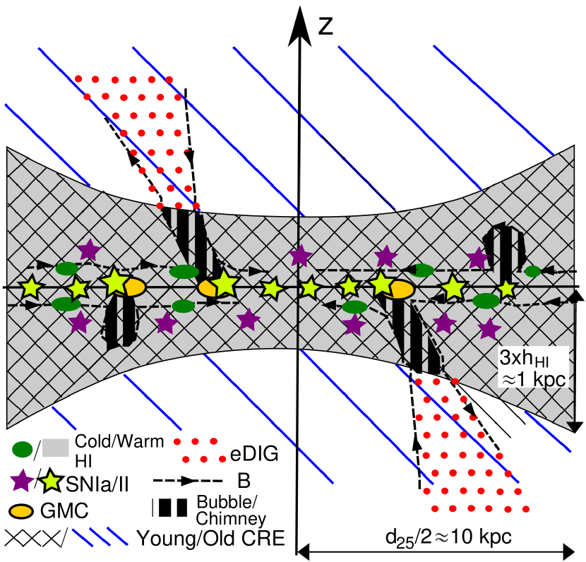
Figure 1: A diagram of the disc–halo interface in galaxies with $\Sigma_{\rm SFR}\ll 10^{-1}~{}\rm M_{\sun}\,yr^{-1}\,kpc^{-2}$. CREs are injected in the disc plane by Type II SNe (and Type Ib/Ic) and in the halo by Type Ia SNe. They accumulate in superbubbles which can break out from the flaring disc of warm H i and form a ‘chimney’, which are cospatial with plumes of extra-planar diffuse ionized gas (eDIG). The magnetic field (dashed lines with arrows) is anchored to the disc in the cold H i clouds. The vertical scale is stretched by a factor of 5.

3.1.2 Disc–halo interface

This paper is about haloes, but in order to investigate them, we need to take into account the full vertical extent of a galaxy, so we give here with a brief overview of the vertical structure of the interstellar medium (ISM). In the context of radio haloes, the transition from the thin to the thick disc is important, so we start with what is commonly referred to as the disc–halo interface. In Fig. 1, we show a conceptual diagram of the disc–halo interface and we discuss in the following how our model can fit into this picture. This diagram is most realistic (although still very simplifying) for galaxies with low $\Sigma_{\rm SFR}\ll 10^{-1}~{}\rm M_{\sun}\,yr^{-1}\,kpc^{-2}$, where cosmic rays are most likely to play a role in launching a wind. Galaxies with higher $\Sigma_{\rm SFR}$ have thermally driven so-called superwinds (Heckman et al., 2000), which are not included in our study (see Adebahr et al., 2013, for a radio continuum study of the superwind galaxy M82).

Cosmic rays are accelerated and injected into the ISM via SNe, where the ejected shells have speeds of the order of 10,000 $\rm km\,s^{-1}$, which create a strong shock while sweeping up material and slowing down. The turbulent magnetic field lines, which surround the shock, deflect the cosmic rays, resulting in an efficient Fermi-type I acceleration with the cosmic rays crossing the shock many times (Bell, 1978). On average, the kinetic energy per SN is $10^{51}$ erg, a few per cent of which is used for the acceleration of cosmic rays (e.g. Rieger et al., 2013). Of the energy stored in the cosmic rays, between 1 and 2 per cent goes into the CREs with the rest into protons and heavier nuclei (e.g. Beck & Krause, 2005). The SNe can be either Type Ia (thermonuclear detonation) or Type II (core-collapse, also Type Ib and Ic). This is of significance since the SNe of Type Ia can occur at galactic heights of a few 100 pc, whereas SNe of other types are restricted to within 100 pc from the midplane (effectively, the scale height of the molecular gas; Ferrière, 2001).

In the thin disc, the CRE population is very diverse. Approximately 10 per cent of the radio continuum emission stems from individual SN remnants, with the remaining 90 per cent made up by the diffuse emission (Lisenfeld & Völk, 2000). The radio spectral index varies strongly between the spiral arms and the inter-arm regions, which is caused by spectral ageing of the CREs with increasing distance from star formation sites (Tabatabaei et al., 2013a; Heesen et al., 2014). Furthermore, CREs can be found within superbubbles, which can be observed during later stages as H i holes with sizes ranging from 100 pc to 2 kpc (Bagetakos et al., 2011). They are the result of dozens of SNe and some of them can contain the CREs long enough that they display a curved non-thermal radio continuum spectrum (Heesen et al., 2015). They may also be the site of ‘chimneys’, where star formation activity in the disc drives advective hot gas flows upward into the halo, carrying magnetic fields along with the hot gas motion and forming cavities in the disk that are observable as H i holes (Heald, 2012). We would expect at any given time a few dozens of superbubbles per galaxy with a diameter of a few 100 pc, so that the volume porosity is a few per cent but can be up to 20 per cent (Bagetakos et al., 2011). It hence becomes clear that the CREs in the thin disc are in fact a superposition of many spectral ages (young CREs in the vicinity of star forming regions, old CREs in the inter-arm regions, young and old CREs in non-thermal superbubbles). Consequently, the radio spectral index of the thin disc is not equivalent to the injection energy spectral index of the CREs as expected from theory, which is $\gamma_{\rm inj}\approx 2$, where the CRE number density is a power-law as function of energy $N\propto E^{-\gamma_{\rm inj}}$, but is steeper. Indeed, the integrated non-thermal radio continuum spectrum of galaxies between 1 and 10 GHz has a spectral index of $\alpha_{\rm nt}\approx-1$, which corresponds to $\gamma_{\rm inj}=3$ (Niklas et al., 1997; Heesen et al., 2014; Basu et al., 2015; Tabatabaei et al., 2017).

In the thick disc, the CRE population becomes more uniform since the distance to the star forming sites becomes more similar and the contrast between spiral arm and inter-arm regions diminishes. The height at which the transition from thin to thick disc happens is probably of the order of a few 100 pc; this is related to the scale height $h_{\rm\text{H\,{i}}}$ of the warm H i disc and thus to the largest height the superbubbles can expand to before they blow-out (at $z=3\times h_{\rm\text{H\,{i}}}$; Mac Low & Ferrara, 1999). The H i discs show a flaring, where the scale height increases with galactocentric distance ($h_{\rm\text{H\,{i}}}=100$–500 pc; Bagetakos et al., 2011), so that the superbubble blow-out would occur at heights between $0.3$ and $1.5$ kpc.

As we will show below, we see the transition from thin to thick disc at a height of 1–2 kpc as traced by a change of the slope in the radio spectral index. Since we cannot really resolve the thin disc, we can only probe the upper limit of the transition height, but our measured values are at least consistent with the described picture. Our first assumption is hence that we fit the radio spectral index in the halo only. In the midplane, the radio continuum emission can be described by a power law with an ‘injection’ spectral index, where this is effectively the spectral index of the diffuse non-thermal radio continuum emission.

3.1.3 Magnetic field structure

The magnetic field in galaxy discs is in approximate energy equipartition with the turbulent gas motions of the (almost) neutral gas and its associated kinetic energy density (Beck, 2016). If the magnetic field is associated with the warm H i disc, as suggested by the superbubble picture, the resulting scale height would be $0.2$–$1.0$ kpc in the thin disc as the magnetic field scale height is a factor of 2 higher than the magnetic pressure scale height. The magnetic field scale height in the thick disc is larger, from equipartition estimates the scale heights are of the order of 4–8 kpc. It is unclear whether the field is associated with either the hot X-ray emitting gas, which has similar scale heights (Strickland et al., 2004; Hodges-Kluck & Bregman, 2013), or the thick H i disc that is seen in some galaxies with scale heights of 2–4 kpc (Zschaechner et al., 2015; Vollmer et al., 2016). We caution though that in both cases accretion from the intergalactic medium probably plays a role as well, so that part of the gas in the halo has a different origin from the magnetic field which is generated by processes within the galaxy.

A discussion of the magnetic field structure would be incomplete without mentioning the results from polarization. The halo field consists of a turbulent and ordered component, with the ordered component having the larger scale height. The turbulent component possibly stems from Parker-type loops, which form when buoyant superbubbles inflated with cosmic rays rise from the disc and opposing magnetic field lines reconnect at its base. This allows a closed magnetic field line to detach from the disc magnetic field (Parker, 1992). In that case the trajectory of the loop would be ballistic, such as for clouds of H i gas in a ‘Galactic fountain’. The ordered magnetic field could be from blown-out superbubbles, where the magnetic field opens up in the halo, with overlapping bubbles in the thick disc creating the halo field (Heald, 2012; Mao et al., 2015; Mulcahy et al., 2017). An alternative scenario is that the turbulent magnetic field is generated in the thin disc by the small-scale dynamo, driven by star-formation related turbulence, and advected into the halo by the wind. A lateral pressure gradient or a galactic wind would then be able to shape the field lines into the often observed X-shaped pattern (e.g. Dahlem et al., 1997; Tüllmann et al., 2000; Krause et al., 2006; Heesen et al., 2009b; Krause, 2009; Soida et al., 2011; Mora & Krause, 2013; Chyży et al., 2016). Such a magnetic field structure has been also seen in models of lagging magnetized haloes (Henriksen & Irwin, 2016). Of course, our simple model cannot take all of this into account, and we attempt in this work only to fit for the total magnetic field strength in the halo, neglecting this sub-division.

Our second assumption is hence, that the magnetic field strength can be described by a two-component exponential function. In the thin disc, the magnetic field strength is regulated by the pressure of the warm H i gas, which has an exponential distribution. This is expected for a constant velocity dispersion in a constant gravity field as found near the midplane. In the thick disc, the dominating turbulent magnetic field is in pressure equilibrium with either the hot X-ray emitting gas or the thick H i disc. If the halo gas is in a hydrostatic equilibrium, the density distribution is close to an exponential function. This is corroborated by observations of the soft X-ray emission in nearby galaxies, which showed that the vertical distribution of the hot ionized gas can be best described by an exponential function, rather than a Gaussian or a power-law function (Strickland et al., 2004). This suggests that X-ray haloes are ‘hot atmospheres’ surrounding galaxies. If the magnetic field is frozen into the ionized plasma, the magnetic field strength will relate to the ionized gas density, so that exponential magnetic fields can be expected.

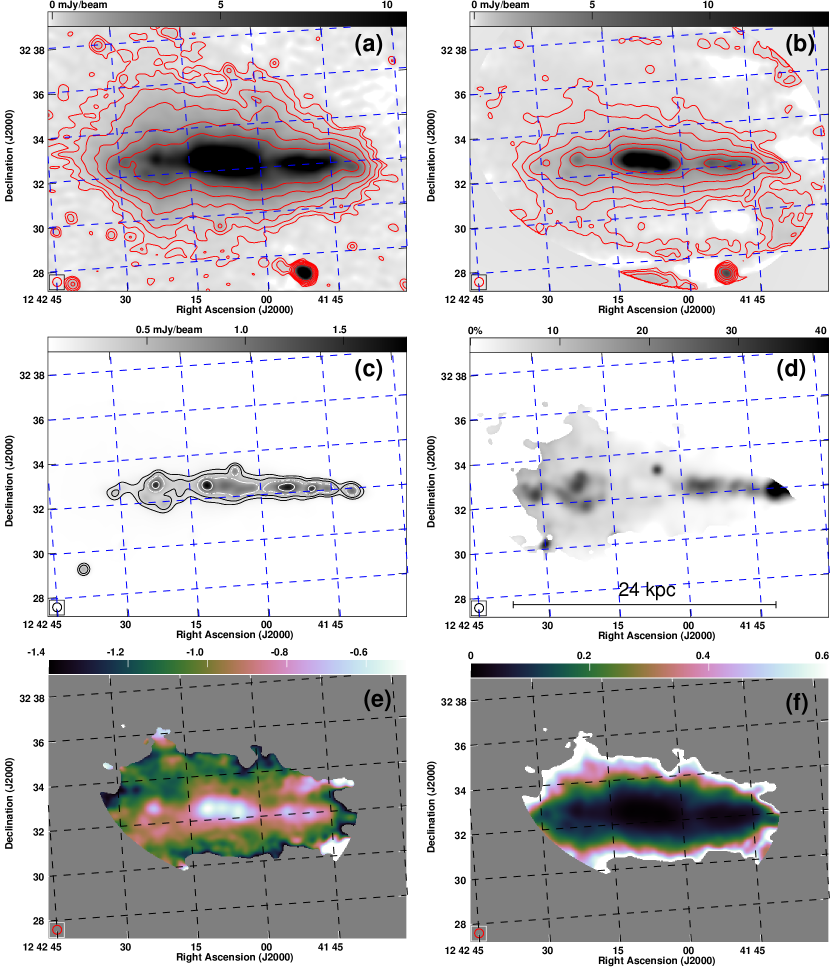
Figure 2: NGC 4631. (a) and (b) radio continuum emission at $1.37$ and $4.86$ GHz, respectively. The high noise level near the edge of the $4.86$-GHz map stems from the correction for the primary beam attenuation of the VLA. (c) the thermal radio continuum emission at $4.86$ GHz. Contours in panels (a)–(c) are at (3, 6, 12, 24, 48 and 96) $\times~{}\sigma$, where $\sigma$ is the rms map noise. In panel (c), the same contour levels as in (b) are used to ease the comparison. (d) thermal fraction at $4.86$ GHz, where they grey-scale ranges from 0 to 40 per cent. (e) non-thermal radio spectral index between $1.37$ and $4.86$ GHz, where the colour-scale ranges from $-1.4$ to $-0.5$. (f) error of the non-thermal radio spectral index, where the colour-scale ranges from 0 to $0.6$. In all panels, the synthesized beam is shown in the bottom left corner and the maps are rotated so that the major axis is horizontal.

3.2 Cosmic-ray transport equations

We are using 1D transport equations for the CRE number density $N(E,z)$, where $E$ is the CRE energy and $z$ is the distance to the midplane. We assume a fixed inner boundary condition with $N(E,0)=N_{0}E^{-\gamma_{\rm inj}}$, where $\gamma_{\rm inj}$ is the injection CRE energy spectral index and $N_{0}$ is a normalization constant. The transport equation for advection is:

$$\frac{\partial N(E,z)}{\partial z}=\frac{1}{V}\left\{\frac{\partial}{\partial E}\left[b(E)N(E,z)\right]\right\}\qquad({\rm Advection}),$$ (3)

where $V$ is the advection speed, assumed here to be constant. Similarly, for diffusion we have:

$$\frac{\partial^{2}N(E,z)}{\partial z^{2}}=\frac{1}{D}\left\{\frac{\partial}{\partial E}\left[b(E)N(E,z)\right]\right\}\qquad({\rm Diffusion}),$$ (4)

where we parametrize the diffusion coefficient as function of the CRE energy as $D=D_{0}E_{\rm GeV}^{\mu}$, where $E_{\rm GeV}$ is the CRE energy in units of GeV and $D_{0}$ is the diffusion coefficient at 1 GeV. We assume $\mu=0.5$ in agreement with what is used for modelling the Milky Way (Strong, Moskalenko & Ptuskin, 2007). There is some debate as to whether this energy dependence applies to CREs with energies of a few GeV (e.g. Recchia et al., 2016a; Mulcahy et al., 2016), but using $\mu=0$ instead changes the results only slightly and we cannot distinguish with our data one way or the other (see also HD16). The combined synchrotron and IC loss rate for CREs is given by (e.g. Longair, 2011):

$$-\left(\frac{{\rm d}E}{{\rm d}t}\right)=b(E)=\frac{4}{3}\sigma_{\rm T}c\left(\frac{E}{m_{\rm e}c^{2}}\right)^{2}(U_{\rm rad}+U_{\rm B}),$$ (5)

where $U_{\rm rad}$ is the radiation energy density, $U_{\rm B}$ is the magnetic field energy density, $\sigma_{\rm T}=6.65\times 10^{-25}~{}\rm cm^{2}$ is the Thomson cross-section and $m_{\rm e}=511~{}\rm keV\,c^{-2}$ is the electron rest mass.

The radiation energy density is the sum of the cosmic microwave background (CMB) radiation energy density and the interstellar radiation field (IRF) energy density; the latter includes contributions from starlight radiation energy density and the total infrared radiation energy density from emission by dust. The magnetic field strength $B_{0}$ in the midplane was calculated from energy equipartition (Beck & Krause, 2005). The energy density of the magnetic field is then $U_{\rm B}=B^{2}/(8\pi)$. Furthermore, we assumed that the ratio $U_{\rm IRF}/U_{\rm B}$ is constant everywhere. The resulting values of these calculations can be found in Table 6 and the details of the calculations are explained in Appendix A.

We assume a two-component exponential magnetic field distribution:

$$B(z)=B_{1}\cdot\exp(-|z|/h_{\rm B1})+(B_{0}-B_{1})\cdot\exp(-|z|/h_{\rm B2}).$$ (6)

Here, $h_{\rm B1}$ and $h_{\rm B2}$ are the magnetic field scale heights in the thin and thick disc, respectively, $B_{0}$ is the magnetic field strength in the midplane and $B_{1}$ is the magnetic field strength of the thin disc component. Equations (3) and (4) are integrated numerically from the inner boundary, so that no outer boundary condition is required. In order to calculate the non-thermal radio continuum intensities the CRE number density is convolved with the synchrotron emission profile of an individual CRE (see HD16 for details).

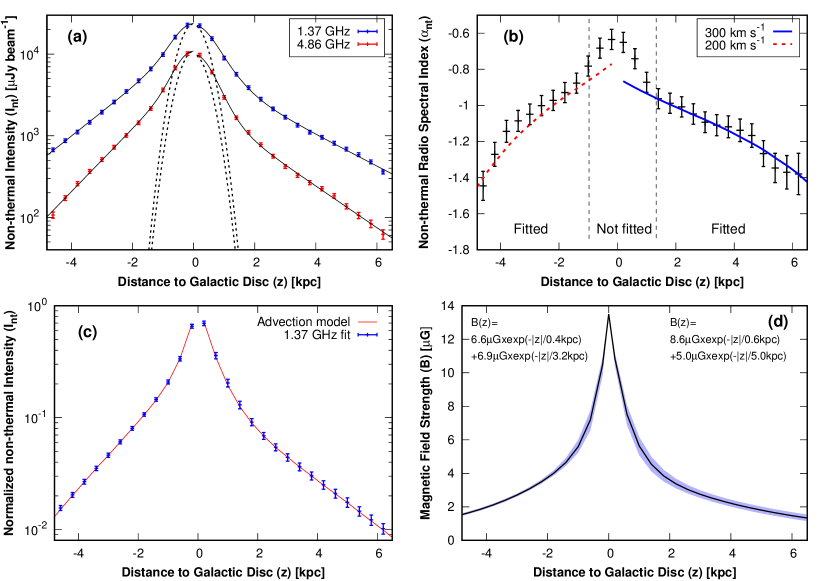
Figure 3: Vertical profiles in NGC 4631. (a) non-thermal radio continuum intensities at $1.37$ and $4.86$ GHz. We fitted a two-component exponential function (solid line) to the profiles. Black dashed lines show the effective beam, which is $I_{\rm beam}(z)=\exp(-z^{2}/(2b^{2}))$ (see Section 3.3.1) (b) non-thermal radio spectral index between $1.37$ and $4.86$ GHz. Lines show the best-fitting advection models, with an advection speed of $300~{}\rm km\,s^{-1}$ in the northern halo (blue solid line) and $200~{}\rm km\,s^{-1}$ in the southern halo (red dashed line). (c) normalized non-thermal intensity model profile at $1.37$ GHz, which is deconvolved from the synthesized beam. The red line shows the intensities of the best-fitting advection model. (d) model of the magnetic field strength with uncertainties (blue-shaded area). Distances $z>0$ refer to the northern halo and distances $z<0$ to the southern one. In panels (a)–(c), the size of the symbols is equivalent to the size or the error bars.

3.3 Fitting procedure

3.3.1 Vertical intensity profiles

In this section, we outline the fitting procedure of the cosmic-ray transport models, where present a step-by-step analysis of NGC 4631. In Fig. 2, we show the radio continuum maps of NGC 4631 – a galaxy that has one of the most impressive radio haloes. We have created vertical profiles of the non-thermal radio continuum intensity, which we present in Fig. 3(a).

In our work, the scale height of the thin disc is comparable to the spatial resolution of the maps. This is why we use the analytical functions of Dumke et al. (1995) that convolve the Gaussian point-spread function (PSF) with either exponential or Gaussian intensity distributions. This Gaussian PSF is exact for interferometric maps and it is a good approximation for single-dish maps. Furthermore, it has become ‘standard practice’ to include a contribution of the inclined disc (if $i<90\degr$), measuring a Gaussian radio intensity distribution along the major axis and projecting that on to the minor axis. This larger PSF is then referred to as the ‘effective beam’ (e.g. Heesen et al., 2009a; Adebahr et al., 2013).

We fit two-component exponential and Gaussian functions to vertical non-thermal intensity profiles, which we present as solid and dashed lines, respectively (see Appendix B for details). For this galaxy, a two-component exponential function fits better than a two-component Gaussian function with a reduced $\chi^{2}_{\rm exp}=0.4$ as opposed to $\chi^{2}_{\rm Gauss}=3.0$ (average of the northern and southern halo at both frequencies). Using the fits to the data, we create vertical non-thermal intensity model profiles using either of the two frequencies, depending which data has the better quality. We calculate the error bars using the uncertainties of the maxima and scale heights of the thin and thick discs (see Appendix B for details).

In Fig. 3(b), we show the vertical profile of the non-thermal spectral index in NGC 4631. The spectral index is fairly flat in the midplane with $\alpha\approx-0.7$ and steepens in the halo to values of $\alpha\approx-1.4$. The profile shows a conspicuous ‘shoulder’, where the spectral index slope flattens at heights $|z|\gtrapprox 1$ kpc. This distance corresponds to the transition from the thin to the thick disc seen in the intensity profiles. We note that the slope of the spectral index profile cannot be resolved in the thin disc because the effective beam is too large. Furthermore, we are overestimating the non-thermal radio spectral index in the thin disc since we did not correct the Balmer H $\alpha$ line emission for internal absorption due to dust (Section 2.2). In the halo, however, these influences can be neglected, so that we can study the spectral index profile there. In order to illustrate the influence of the effective beam, we have shown its contribution to the vertical intensity profile in Fig. 3(a); in case of NGC 4631 we restrict the fitting of the spectral index to $|z|\geq 1.4$ kpc. We show the fitting areas for the rest of the sample in Appendix D. In NGC 55 and 253, the fitting area has also an outer limit, because the $L$ band maps are affected by missing fluxes (Section 2.1.6). In NGC 253, we do not exclude this thin disc in the fit since we do not resolve it in the spectral index anyway and there would be otherwise not enough data points for a meaningful fit.

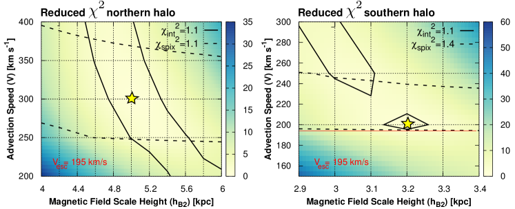
Figure 4: NGC 4631. Reduced $\chi^{2}$ of the advection model fitting in the thick disc as function of magnetic field scale height and the advection speed. The colour scale shows $\chi^{2}=\chi^{2}_{\rm int}+\chi^{2}_{\rm spix}$, where $\chi^{2}_{\rm int}$ refers to the model intensity profile (Fig. 3c) and $\chi^{2}_{\rm spix}$ refers to the spectral index profile (Fig. 3b). Solid lines show $\chi^{2}_{\rm int,min}+1$ and dashed lines show $\chi^{2}_{\rm spix,min}+1$. The best-fitting models (with uncertainties) lie in the intersection of the two contours and are marked by yellow stars. The left panel is for the northern halo ($z>0$) and the right one for the southern halo ($z<0$). The red line shows the escape velocity near the midplane ($V_{\rm esc}=\sqrt{2}\times V_{\rm rot}$).

3.3.2 Finding the best-fitting model

We simultaneously fit for the advection speed (or diffusion coefficient), the magnetic field scale height and the injection spectral index. In order to find an ‘initial guess’, we first vary the magnetic field profile to fit the intensity model at one frequency, varying the scale height and choosing an advection speed (or diffusion coefficient) that approximately fits the spectral index profile (together with the chosen injection spectral index). For NGC 4631, we show the best-fitting advection intensity profile in Fig. 3(c) and the best-fitting advection spectral index profile in Fig. 3(b). The corresponding vertical profile of the magnetic field strength is shown in Fig. 3(d). The error interval of the latter stems from the uncertainties of the magnetic field scale heights in the thin and thick disc, it does not include any uncertainty from the total magnetic field strength estimate from the equipartition assumption (we discuss the influence of the equipartition estimate in Section 5.3). The magnetic field strength decreases rapidly and reaches a value of approximately half the maximum field strength at $|z|=1$ kpc from where on it decreases more slowly.

From the best-fitting model we can work out the uncertainties of the advection speed and magnetic field strength. This is shown in Fig. 4, where we plot the reduced $\chi^{2}$ for both the intensity and spectral index fitting in NGC 4631. The fitting of the intensities depends almost exclusively on the magnetic field profile, although a higher advection speed can offset a lower magnetic field scale height. In contrast, the fitting of the spectral index profile depends mostly on the advection speed and hardly on the magnetic field scale height. This means that best-fitting areas are almost perpendicularly aligned, so that the advection speed and magnetic field scale height can be constrained well by a simultaneous fit.

4 Results

In Table 7, we present non-thermal intensity scale heights in the thick disc at $L$ and $C$ band, magnetic field scale heights in the thin and thick discs, advection speeds and diffusion coefficients for the entire sample. In some cases, we could find a best-fitting value for the magnetic field scale height and/or advection speed, but not an upper and/or lower limit. For these values, the given error interval is a lower limit; they are plotted in Fig. 5 for the parameter studies with arrows denoting the error bars, but are not taken into account for the statistical analysis. Maps and plots are presented in Appendix D.

4.1 The distinction between advection and diffusion

At first we present our findings whether the cosmic-ray transport in haloes is advection- or diffusion-dominated. We note that this distinction is a common one since advection will take over diffusion in the halo quickly if there is a galactic wind (Ptuskin et al., 1997; Recchia et al., 2016b). The effective boundary $s_{\star}$ at which ($|z|>s_{\star}$) advection dominates over diffusion is:

$$\frac{s_{\star}^{2}}{D}\approx\frac{s_{\star}}{V}\Rightarrow s_{\star}\approx 0.3\times\frac{D_{28}}{V_{100}}~{}\rm kpc,$$ (7)

where $D_{28}$ is the diffusion coefficient in units of $10^{28}~{}\rm cm^{2}\,s^{-1}$ and $V_{\rm 100}$ is the advection speed in units of $100~{}\rm km\,s^{-1}$. Diffusion coefficients in galaxies have values of a few $10^{28}~{}\rm cm^{2}\,s^{-1}$ (e.g. Berkhuijsen et al., 2013; Tabatabaei et al., 2013b; Mulcahy et al., 2014; Mulcahy et al., 2016) in agreement with the Milky Way value of $3\times 10^{28}~{}\rm cm^{2}\,s^{-1}$ (Strong et al., 2007). For a diffusion coefficient of $3\times 10^{28}~{}\rm cm^{2}\,s^{-1}$ and an advection speed of $200~{}\rm km\,s^{-1}$, the transition happens at a height of $0.45~{}\rm kpc$. Hence, it is justified to assume an advection only model in the halo if there is a wind.

If there is no wind, the radio halo may be diffusion dominated. As HD16 showed, the vertical profile of the radio spectral index can be used in order to distinguish between advection and diffusion. Advection has spectral index profiles, which gradually steepen as function of height. In contrast, diffusion leads to spectral index profiles that steepen only very little at small heights, but have steep cut-offs at large heights. This is caused by a steep cut-off of the CRE number density at large heights in case of diffusion, which reflects the fact that the CREs cannot escape the galaxy. Thus, the vertical diffusion spectral index profiles have ‘parabolic’ shapes, which should distinguish them from the ‘linear’ advection profiles. In practice it can, however, be difficult to allow for a distinction since the uncertainties of the radio spectral index are too large. Therefore, we fitted all our galaxies with both an advection and diffusion model.

Table 7: Non-thermal intensity scale height $z_{0}$ at $L$ and $C$ band, advection speed $V$, diffusion coefficient $D_{0}$ ($D=D_{0}E_{\rm GeV}^{0.5}$) and magnetic field scale height of the thin ($h_{\rm B1}$) and thick disc ($h_{\rm B2}$) in the northern (N) and southern (S) halo.

Galaxy	$z_{0}$ ($L$/N)a	$z_{0}$ ($C$/N)b	$z_{0}$ ($L$/S)c	$z_{0}$ ($C$/S)d	$h_{\rm B1}$ (N)e	$h_{\rm B1}$ (S)f	$h_{\rm B2}$ (N)g	$h_{\rm B2}$ (S)h	$V$ (N)i	$V$ (S)j
	(kpc)	(kpc)	(kpc)	(kpc)	(kpc)	(kpc)	(kpc)	(kpc)	($\rm km\,s^{-1}$)	($\rm km\,s^{-1}$)
NGC 55	$2.03\pm 1.46$	$1.72\pm 0.22$	$1.06\pm 0.14$	$2.01\pm 0.71$	$0.3\pm 0.1$	$0.2\pm 0.1$	$4.0^{++2.0}_{-1.2}$	$2.5^{+0.8}_{-0.7}$	$150^{++200}_{--100}$	$100^{+80}_{-10}$
NGC 253	$1.26\pm 0.07$	$1.14\pm 0.04$	$1.33\pm 0.04$	$1.28\pm 0.02$	N/A	N/A	$2.8^{+0.2}_{-0.7}$	$3.0^{+0.1}_{-0.5}$	$400^{+200}_{-20}$	$500^{++400}_{-120}$
NGC 891	$1.33\pm 0.02$	$1.30\pm 0.02$	$1.25\pm 0.01$	$1.24\pm 0.03$	$0.1\pm 0.1$	$0.2\pm 0.1$	$3.0^{+0.2}_{-0.2}$	$2.5^{+0.2}_{-0.2}$	$600^{++600}_{-200}$	$600^{++600}_{-200}$
NGC 3044	$3.64\pm 0.95$	$1.47\pm 0.26$	$1.30\pm 0.08$	$1.15\pm 0.14$	$0.5\pm 0.1$	$0.5\pm 0.1$	$4.5^{++4.5}_{-1.7}$	$3.0^{+0.7}_{-0.6}$	$200^{++200}_{--100}$	$200^{+200}_{-50}$
NGC 3079	$5.14\pm 8.86$	$1.00\pm 0.19$	$3.41\pm 0.63$	$1.54\pm 0.10$	$1.2\pm 0.1$	$1.0\pm 0.1$	$4.5^{+7.5}_{-2.0}$	$8.0^{+7.0}_{-3.0}$	$300^{+80}_{-40}$	$400^{+80}_{-80}$
NGC 3628	$1.23\pm 0.05$	$1.16\pm 0.04$	N/A	$0.87\pm 0.02$	$0.1\pm 0.1$	$0.1\pm 0.1$	$2.6^{+0.3}_{-0.3}$	$2.0^{+0.1}_{-0.3}$	$250^{+250}_{-50}$	$250^{++400}_{-50}$
NGC 4565	$1.90\pm 0.10$	$1.63\pm 0.07$	$3.11\pm 0.66$	$1.75\pm 0.10$	N/A	$0.8\pm 0.1$	$3.5^{+1.1}_{-0.5}$	$4.0^{+0.2}_{-0.7}$	$500^{++300}_{-220}$	$250^{+150}_{-20}$
NGC 4631	$2.24\pm 0.07$	$1.70\pm 0.05$	$1.47\pm 0.02$	$1.13\pm 0.02$	$0.6\pm 0.1$	$0.4\pm 0.1$	$5.0^{+0.6}_{-0.5}$	$3.2^{+0.1}_{-0.2}$	$300^{+80}_{-50}$	$200^{+50}_{-20}$
NGC 4666	$1.51\pm 0.05$	$1.54\pm 0.03$	$2.01\pm 0.08$	$1.70\pm 0.11$	$0.5\pm 0.1$	$0.5\pm 0.1$	$3.0^{+0.3}_{-0.3}$	$4.0^{+0.4}_{-0.5}$	$700^{++200}_{-100}$	$500^{+80}_{-70}$
NGC 5775	$2.72\pm 0.12$	$1.27\pm 0.06$	$1.91\pm 0.12$	$2.03\pm 0.80$	$1.0\pm 0.1$	$0.4\pm 0.1$	$7.0^{+1.5}_{-1.0}$	$4.0^{++2.0}_{-0.8}$	$400^{+100}_{-50}$	$450^{++100}_{--150}$
NGC 7090	$2.07\pm 0.18$	$1.96\pm 0.50$	$1.53\pm 0.39$	$1.14\pm 0.44$	$0.6\pm 0.1$	$0.4\pm 0.1$	$5.5^{+1.0}_{-1.2}$	$4.5^{+3.5}_{-2.7}$	$200^{+310}_{-10}$	$300^{++300}_{-120}$
NGC 7462	$1.62\pm 0.15$	$1.38\pm 0.03$	$1.50\pm 0.03$	$1.46\pm 0.01$	N/A	N/A	$3.0^{+1.0}_{-0.2}$	$3.5^{+0.7}_{-0.5}$	$<80$	$<100$
							$h_{\rm B2}$ (N)g	$h_{\rm B2}$ (S)h	$D_{0}$ (N)i	$D_{0}$ (S)j
							(kpc)	(kpc)	($\rm 10^{28}cm^{2}\,s^{-1}$)
NGC 7462							$3.0^{+1.0}_{-0.2}$	$3.5^{+0.7}_{-0.5}$	$2.2^{+0.4}_{-0.4}$	$2.6^{+0.1}_{-0.6}$

We find that only NGC 7462 can be fitted with a diffusion coefficient roughly in agreement of what we would expect, namely $D_{0}\approx 3\times 10^{28}~{}\rm cm^{2}\,s^{-1}$. All other galaxies required values in excess of this, with values between $1.2\times 10^{29}~{}\rm cm^{2}\,s^{-1}$ (NGC 55) and $4\times 10^{30}~{}\rm cm^{2}\,s^{-1}$ (NGC 4666). There is no physical reason why the diffusion coefficient should deviate so much from the Milky Way value, because the magnetic field structure is not too dissimilar. Such high diffusion coefficients would also lead to the cosmic rays leaving the galaxy without interaction, so that they do not transfer energy and momentum to the ionized gas. This is at odds with cosmic-ray driven wind models, which now have become very popular (e.g. Breitschwerdt et al., 1991; Everett et al., 2008; Samui et al., 2010; Salem & Bryan, 2014). Their advantage over previous models is that they can explain the existence of winds in galaxies with $\Sigma_{\rm SFR}\ll 10^{-1}~{}\rm M_{\sun}\,yr^{-1}\,kpc^{-2}$, where thermally driven winds suffer from too strong radiative cooling. Thus, we rule out models with $D_{0}>10^{29}~{}\rm cm^{2}\,s^{-1}$ and assume that haloes are in this case advection dominated.

4.2 Non-thermal intensity scale heights

We find that the vertical non-thermal intensity profiles in 7 out of the 12 sample galaxies are better fitted by exponential rather than Gaussian functions, where $\chi^{2}_{\rm exp}-\chi^{2}_{\rm Gauss}\leq-1$ (NGC 55, 891, 3044, 3079, 3628, 4631 and 5775; the reduced $\chi^{2}$ values are the average of the northern and southern halo at both frequencies). In 3 galaxies the fits are of equivalent quality, where $-1<\chi^{2}_{\rm exp}-\chi^{2}_{\rm Gauss}<1$ (NGC 253, 4565 and 7090). Only in 1 galaxy the Gaussian fits significantly better than the exponential function, where $\chi^{2}_{\rm exp}-\chi^{2}_{\rm Gauss}\geq 1$ (NGC 7462). In 10 out of the 11 exponential haloes (including the 7 better and the 3 equivalent fits) we also detect a thin disc component. Only in NGC 4565 this is not the case, which we believe is due to a combination of low spatial resolution and disc intensity (NGC 4565 has the lowest average surface intensity). We detect a thick disc in the Magellanic-type galaxy NGC 55 (Appendix D), the first report of a radio halo in this galaxy.

Averaged across the sample, the exponential scale height of the thin disc is $0.41\pm 0.21$ kpc at $1.4$ GHz and $0.25\pm 0.13$ kpc at 5 GHz. The scale height of the thick disc is $1.33\pm 1.25$ kpc at $1.4$ GHz and $1.22\pm 0.43$ kpc at 5 GHz; these values are in excellent agreement with those of Krause et al. (2017). We found a large variety of scale heights at $1.4$ GHz ranging between $1.2$ kpc and $2.7$ kpc (excluding values with fractional errors larger than 10 per cent). At 5 GHz the scale heights of the thick disc vary between $0.9$ and $2.0$ kpc. In NGC 7462, we find only a thick Gaussian disc with a scale height of $\approx$$1.5$ kpc at both $1.4$ and 5 GHz.

In Fig. 5, we show the dependence of the 5-GHz intensity scale heights as function of the SFR, $\Sigma_{\rm SFR}$ and $V_{\rm rot}$. These are log–log diagrams so that we can fit linear functions to them, which are representative of power-laws. We find no correlation between the intensity scale height and either parameter (Spearman’s rank correlation coefficient $|\rho_{\rm s}|\leq 0.33$). Full results of the scale height fitting are presented in Appendix B.

4.3 Non-thermal radio spectral indices

We find that in those 7 galaxies that have both a thin and a thick disc, the vertical non-thermal radio spectral index profile shows the thin and the thick disc clearly separated as well (NGC 55, 891, 3044, 3628, 4631, 5775 and 7090). The exceptions are NGC 253, 4565 and 4666, where the thin and the thick disc are difficult to separate in the intensity profiles. This is caused by either low inclination angles ($<$$79\degr$ in NGC 253 and 4666) or low spatial resolution ($2.1$ kpc in NGC 4565). In NGC 3079, we can separate the thin and the thick disc in the intensity profile, but the slope of the spectral index profile in the thick disc is so high that there is no visible transition from the thin to the thick disc. Even though we have masked the nuclear outflow, it is possible that additional diffuse emission associated with it can contaminate our radio continuum emission. Since this is more pronounced at $L$ band, where the scale heights in the thick radio discs are the largest in our sample, old CREs, possibly stemming from an earlier episode of AGN activity, could be responsible for this emission. Such emission can also be explained as the result of jet interactions with clumpy media (Middelberg et al., 2007), which can contaminate the radio emission around the thin/thick disc transition. In all galaxies, the non-thermal radio spectral index in the thick disc varies between $-1.4$ and $-1.0$, showing that spectral ageing of the CREs plays an important role in the halo.

The integrated non-thermal radio spectral indices range from $-1.3$ (NGC 7462) to $-0.6$ (NGC 55). The significance of the integrated non-thermal spectral index is that we can infer which energy losses of the CREs are dominating. If synchrotron and IC radiation losses are important, the CRE spectrum is $N(E,z)\propto E^{-\gamma_{\rm inj}-1}$. If, on the other hand, adiabatic losses dominate or the CREs escape freely, the CRE spectrum is unchanged from the injection spectrum with $N(E,z)\propto E^{-\gamma_{\rm inj}}$ (Lisenfeld & Völk, 2000; Longair, 2011). In case radiation losses are important, a galaxy is referred to as an electron calorimeter, where the CREs are losing their energy before they can escape through radiation and ionization losses (Yoast-Hull et al., 2013).

This shows that NGC 55 is not an electron calorimeter, whereas NGC 7462 is one. NGC 55 is a Magellanic-type dwarf irregular galaxy and possibly has a strong wind, similar to the starburst dwarf irregular galaxy IC 10 (Chyży et al., 2016). On the other hand, NGC 7462 is diffusion-dominated (no wind) and all the CREs are confined in the halo, leading to high CRE radiation losses. Our finding that galaxies have galactic winds means that galaxies are in general not electron calorimeters. This has some consequences for the radio continuum–SFR relation and its close corollary the radio continuum–far-infrared relation, which we discuss in Section 5.2.

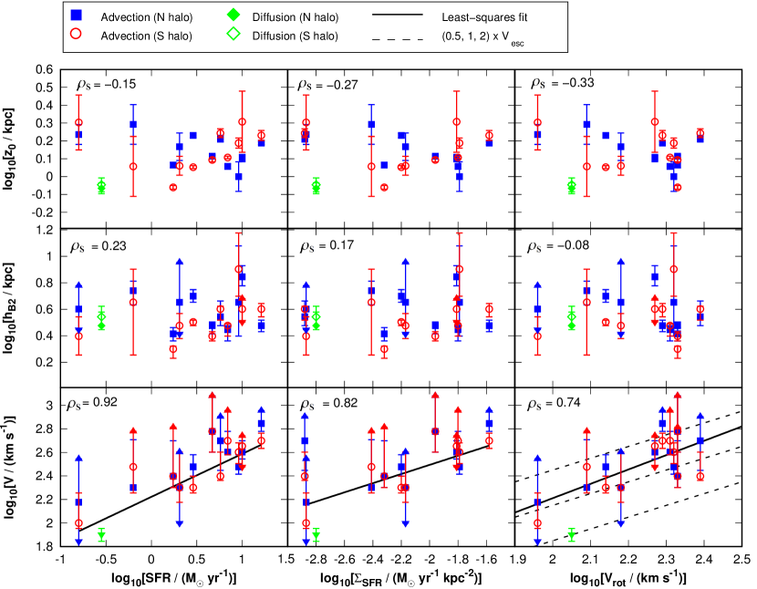
Figure 5: Parameter studies in log–log diagrams as function of SFR, SFR surface density ($\Sigma_{\rm SFR}$) and rotation speed $V_{\rm rot}$. Top panels: non-thermal intensity scale height ($z_{0}$) at 5 GHz ($8.5$ GHz for NGC 5775) of the thick radio disc. Middle panels: magnetic field scale height ($h_{\rm B2}$) of the thick radio disc. Bottom panels: Advection speed ($V$), where solid lines show least-squares fits. In the bottom right panel the dashed lines show ($0.5$, 1, 2)$\times V_{\rm esc}$. In each panel, we also present Spearman’s rank correlation coefficient, $\rho_{\rm s}$, which we derived from values that have both an upper and lower limits.

4.4 Magnetic field scale heights

In the thin disc, magnetic field scale heights range from $0.1$ kpc in NGC 3628 to $1.2$ kpc in NGC 3079. Averaged across the sample, the magnetic field scale height in the thin disc is $0.50\pm 0.32$ kpc (assuming an error of $0.1$ kpc for each measurement). In the thick disc, we find scale heights between 2 kpc in NGC 3628 and 8 kpc in NGC 3079. In Fig. 5 we show that the magnetic field scale height of the thick disc does not depend on either SFR, $\Sigma_{\rm SFR}$ or $V_{\rm rot}$. The magnetic field in the halo must be regulated by something else than the wind driven by the star formation in the disc. Maybe the geometry plays a role, as for instance predicted by the flux tube model used in the aforementioned 1D cosmic-ray driven wind models. The large scale heights in NGC 3079 can possibly be explained by the strong interaction of this galaxy with nearby group members (Shafi et al., 2015). Tidal interaction can ‘puff’ up the thin and the thick discs by inflating the warm neutral medium, which in our picture results in a larger magnetic field scale height. Alternatively, the prominent starburst/AGN-driven nuclear outflow advects cosmic rays and magnetic fields, so that the magnetic field extends further into the halo (Cecil et al., 2001; Middelberg et al., 2007).

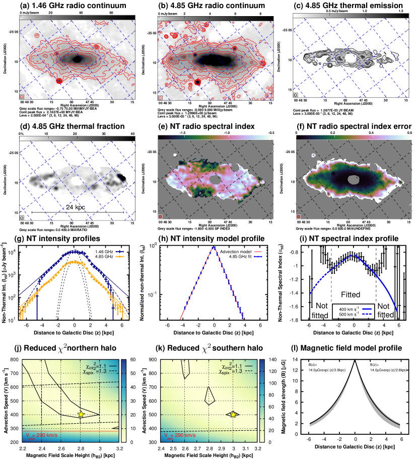
Figure 10: NGC 253. (a) radio continuum emission at $1.46$ GHz. (b) radio continuum emission at $4.85$ GHz. (c) thermal radio continuum emission at $4.85$ GHz. Contours in panels (a)–(c) are at (3, 6, 12, 24, 48 and 96) $\times\sigma$, where $\sigma$ is the rms map noise. In panel (c), the same contour levels as in (b) are used. (d) thermal fraction at $4.85$ GHz, where the grey-scale ranges from 0 to 40 per cent. (e) non-thermal radio spectral index between $1.46$ and $4.85$ GHz, where the colour scale ranges from $-1.8$ to $-0.5$. (f) error of the non-thermal radio spectral index, where the colour scale ranges from 0 to $0.6$. Panels (a)–(f) are rotated so that the major axis ($PA=52\degr$) is horizontal and the synthesized beam is shown in the bottom left corner. (g) vertical non-thermal intensity profiles at both frequencies, where solid lines show two-component exponential fits and dashed lines two-component Gaussian fits. (h) normalized vertical non-thermal intensity model profile at $4.85$ GHz with best-fitting advection model. (i) vertical non-thermal radio spectral index profile with best-fitting advection model. (j) reduced $\chi^{2}$ in the northern halo as function of advection speed and magnetic field scale height in the thick disc. (k) same as (j) but in the southern halo. The red line in (j) shows the escape velocity near the midplane. (l) vertical magnetic field model profile.

Averaged across our sample, the magnetic field scale height in the thick disc is $3.0\pm 1.7$ kpc. Compared with the magnetic field scale height predicted by energy equipartition, $h_{\rm B}\approx 4\cdot z_{0}$ (where $z_{0}$ is the 5-GHz intensity scale height) for $\alpha_{\rm nt}\approx-1$, the magnetic field scale height in the thick disc is 35 per cent lower. This is because the vertical decrease of the CRE number density is smaller than that of the magnetic field energy density (fig. 10 in HD16).

4.5 Advection speeds

The advection speeds range from $100~{}\rm km\,s^{-1}$ in NGC 55 to $700~{}\rm km\,s^{-1}$ in NGC 4666. The advection speeds rise as $V\propto\rm SFR^{0.36\pm 0.06}$ and $V\propto\rm\Sigma_{\rm SFR}^{0.39\pm 0.09}$ as shown in Fig. 5. We found Spearman’s rank correlation coefficients of $\rho_{\rm s}=0.92$ and $\rho_{\rm s}=0.82$, respectively; for this we used a least-squares fitting routine in the log–log diagram, taking only data points with both upper and lower limits into account (that have no arrows in Fig. 5). These correlations are robust with respect to performing the ‘jackknife’ test, where we leave out NGC 55, the galaxy with the lowest SFR. We find another possible correlation with $V_{\rm rot}$, which is, however, not robust to the jackknife test. We need more observations of dwarf irregular galaxies to measure winds in them. A correlation between advection speed and SFR has been suggested earlier based on the observation that the 5-GHz radio continuum scale height is almost constant and does not depend on the magnetic field strength in the midplane (Krause, 2015). If one assumes that the scale height is a function of the CRE lifetime, neglecting the influence of the magnetic field, then scale height scales as $\propto B_{0}^{-1.5}$, where it is also assumed that synchrotron losses are dominating over IC losses (Appendix A). If one now uses that the magnetic field strength scales as $B_{0}\propto\rm SFR^{0.3}$ (e.g. Heesen et al., 2014), one can conclude that the scale height scales as $\propto\rm SFR^{-0.5}$. Hence, in order to have a constant scale height the advection speed has to scale as $V\propto\rm SFR^{0.5}$ (Krause, 2015). In reality, the magnetic field scale height plays also a role, so that the scaling is somewhat less with the SFR, but the general idea is a valid one.

The advection speeds lie within the range $0.5\leq V/V_{\rm esc}\leq 2$ (including the uncertainties), where $V_{\rm esc}=\sqrt{2}\times V_{\rm rot}$ is the escape velocity near the midplane (further away from the disc, in the dark matter halo, the escape velocity is higher). In NGC 7462, where diffusion dominates, we can calculate an upper limit for the advection speed, by comparing how much advection can contribute at most. This can be done either analytically using equation (7), inserting $s_{\star}=2.5$ kpc, the CRE scale height in NGC 7462 (fig. 10 in HD16), or numerically by comparing profiles of the CRE number density. Both ways give a similar result, namely that the upper limit for the advection speed in NGC 7462 is between 80 and $100~{}\rm km\,s^{-1}$.

Are we tracing really disc winds, or are the radio haloes only extensions to the nuclear outflows seen in galaxies with nuclear star bursts or active galactic nuclei (AGN)? A case in point is NGC 3079, a galaxy with a low-luminosity AGN. On the northern side of the galaxy a nuclear outflow is detected with an outflow speed of the warm ionized gas of up to $\approx$$1000~{}\rm km\,s^{-1}$ (Cecil et al., 2001). There is also a nuclear outflow on the southern side, which can be seen only in the radio continuum due to absorption by dust of the optical emission. A similar outflow, albeit less prominent in the radio continuum, can be seen in the nuclear region of NGC 253 (Heesen et al., 2011; Westmoquette et al., 2011). Here, the nuclear outflow speed is of the order of $\approx$300$~{}\rm km\,s^{-1}$, traced by the Doppler shift of the warm ionized gas. The other galaxies in our sample have not been studied in detail with regards to their nuclear outflows, although the study by Ho et al. (1997) of the [N ii] emission line offers some clues. Our samples have in common NGC 891, 3079, 3628, 4565, 4631 and 5775. Their line widths are all smaller than our advection speeds, with the exception of NGC 3079. In NGC 891, 3628 and 5775 the line-width equivalent velocity is less than 50 per cent of our advection speed. Studying nuclear outflows and determining their kinematics is very challenging and is usually based on the presence of unusually broad or shifted lines (or lines with excess wing emission). Even when such features are identified, it is extremely difficult to distinguish between rotation, inflow, or outflow (often outflows are inferred from the presence of velocities exceeding the escape velocity of the host galaxy). Hence, it is not possible to compare the properties of nuclear outflows and disc winds in detail for our sample.

5 Discussion

5.1 Cosmic-ray driven winds

Our result of increasing advection speeds as function of the SFR is also observed in studies of other low-redshift galaxies, where the wind speed of either the warm ionized gas (e.g. Arribas et al., 2014; Heckman et al., 2015; Heckman & Borthakur, 2016) or the neutral gas (e.g. Martin, 2005; Rupke et al., 2005) is measured. This can be explained by a star-formation driven wind due to a combination of a hot wind fluid driven by the thermalized ejecta of massive stars and radiation pressure. Another explanation is cosmic-ray driven winds, where the cosmic-ray pressure (via Alfvén waves) in conjunction with the pressure of the thermal gas pushes the material outwards. Hybrid forms of winds are also possible. Cosmic-ray driven winds are predominant for galaxies with low $\Sigma_{\rm SFR}$, where the pressure of the thermal gas alone is insufficient to launch a wind (Everett et al., 2008). The influence of the cosmic ray pressure can be tested with our observations: the magnetic field strength in galaxies scales as $B\propto\rm SFR^{0.30\pm 0.02}$ (Heesen et al., 2014), similar to the relation of the advection speeds, which is $V\propto\rm SFR^{0.36\pm 0.06}$. Hence, the magnetic field strength and the advection velocity are nearly proportional to each other. This also means that $V^{2}\propto B^{2}$, so that the kinetic energy density of the wind $U_{\rm kin}=(1/2)\rho V^{2}$ is proportional to the magnetic energy density $U_{\rm B}=B^{2}/(8\pi)$; here, $\rho$ is the density of the hot ionized gas. This may tell us that the wind is driven by cosmic rays, which are roughly in equipartition with the magnetic field.

Another important result is the remarkable agreement between advection speeds and escape velocities. Again, this can be explained by cosmic-ray driven winds. Initially, the wind speed is below the sound speed of the combined thermal and cosmic ray gas (the so-called ‘compound sound speed’), but the flow accelerates in the halo where it goes through the critical point (Mach number $M=1$) at a distance of a few kpc away from the disc. Eventually the wind accelerates further to reach an asymptotic velocity of a few times the escape velocity (Breitschwerdt et al., 1991; Everett et al., 2008). Wind speeds of the order of the escape velocity are also predicted for pressure-driven galactic winds without the contribution from cosmic rays (Murray et al., 2005; Heckman et al., 2015; Heckman & Borthakur, 2016). The accelerating force in momentum-driven winds is a combination of radiation pressure, ram pressure from galactic winds and non-thermal pressure due to magnetic fields and cosmic rays. It is an intriguing possibility that galactic winds are driven by the combined pressure supplied by star formation (via SNe ejecta and stellar winds) and cosmic rays.

Within the critical point, the compound sound speed can be approximated by (Breitschwerdt et al., 1991):

$$c_{\rm comp}^{2}\approx\frac{1}{2}g_{\rm eff}\frac{Z_{0}^{2}}{z_{\rm c}},$$ (8)

where $g_{\rm eff}$ is the gravitational acceleration in the halo, $Z_{0}$ is the height where the flow becomes spherical and $z_{\rm c}$ is the height of the critical point. The gravitational acceleration can be approximated by $g_{\rm eff}\approx V_{\rm rot}^{2}/r_{\star}$ because the flow emanates as a disc wind from radii with active star formation ($r\leq r_{\star}$). We do not know where the critical point lies, but it must be of the order of the magnetic field scale height since our outflow speeds are already exceeding the escape velocity. Hence, setting $z_{\rm c}\approx h_{\rm B}$, we find for the compound sound speed:

$$c_{\rm comp}=V_{\rm rot}\cdot\frac{Z_{0}}{\sqrt{2r_{\star}\cdot h_{\rm B}}}.$$ (9)

With $r_{\star}\approx 10~{}\rm kpc$, $Z_{0}\approx 15~{}\rm kpc$ and $h_{\rm B}\approx 3~{}\rm kpc$, we find $c_{\rm comp}\approx 2\cdot V_{\rm rot}$, in good agreement with our advection speeds. While the exact numerical value of equation (9) is uncertain, the prediction is that the advection speeds of cosmic-ray driven winds scale with the rotation speeds and are similar to the escape velocities.

The particular value of our radio continuum observations lies in the fact that we can measure wind speeds for galaxies with $\Sigma_{\rm SFR}<0.3\times 10^{-1}~{}\rm M_{\sun}\,yr^{-1}\,kpc^{-2}$, whereas conventional absorption and emission line studies have so far focused on galaxies exceeding this limit. All of our sample galaxies fulfil $\Sigma_{\rm SFR}>10^{-3}~{}\rm M_{\sun}\,yr^{-1}\,kpc^{-2}$, for which Rossa & Dettmar (2003a) detect extra-planar diffuse ionized gas (eDIG). Only in NGC 7462, which has $\Sigma_{\rm SFR}=1.6\times 10^{-3}~{}\rm M_{\sun}\,yr^{-1}\,kpc^{-2}$, we find a diffusion-dominated halo. This galaxy is only marginally above the $\Sigma_{\rm SFR}$-threshold. This leaves the possibility that galaxies with no eDIG are diffusion-dominated and have no outflows in them, whereas galaxies with eDIG are advection-dominated and have outflows. We need to extend this kind of study to galaxies with lower $\Sigma_{\rm SFR}$ to confirm this theory.

5.2 Radio–SFR relation

Radio continuum emission in galaxies emerges from two distinct processes: thermal free–free (bremsstrahlung) and non-thermal (synchrotron) radiation. Both are related to the formation of massive stars. UV-radiation from massive stars ionizes the ISM, which gives rise to the free–free emission. The explanation of the non-thermal radio continuum emission (which dominates at frequencies below $\approx$30 GHz) is more involved: massive stars end their lives as SNe. When the blast wave of the explosion reaches the ISM, strong shocks are formed, which accelerate protons, nuclei, and electrons. The CREs spiral around the interstellar magnetic field lines, thereby emitting highly linearly polarized synchrotron emission. The relation between the radio continuum luminosity of a galaxy and its SFR (in the following, the radio–SFR relation) is due to the interplay of star formation, CREs and magnetic fields.

The radio–SFR relation is very tight, as Heesen et al. (2014) have shown: using the relation of Condon (1992), and converting $1.4$-GHz radio luminosities into radio derived SFRs, they found agreement within 50 per cent with state-of-the-art star formation tracers, such as far-UV, H $\alpha$ and mid- or far-infrared emission. An even better agreement can be achieved if the radio spectrum is integrated over a wide frequency range (‘bolometric radio luminosity’; Tabatabaei et al., 2017). Moreover, these authors found that the radio luminosity is a non-linear function of the SFR, as predicted by the model of Niklas & Beck (1997) as detailed below. In radio haloes, the spatially resolved radio–SFR relation is super-linear as well if we take the $\lambda$850-$\mu\rm m$ far-infrared emission as a proxy for the SFR (Irwin et al., 2013).

It has been realised early on (Condon, 1992) for the non-thermal radio continuum emission to be related to the SFR, (i) the CREs have either to emit all their energy within a galaxy, so that the galaxy constitutes an electron calorimeter; (ii) or the cosmic rays have to be in energy equipartition with the magnetic field and there is a magnetic field–SFR or magnetic field–gas relation (Niklas & Beck, 1997). Model (i) predicts a linear non-thermal radio–SFR relation, model (ii) a non-linear one. Present-day observations of spiral galaxies favour model (ii), which is expected since galaxies in general are not electron calorimeters. Electron calorimetry might hold at best in starburst galaxies, but almost certainly not in low-mass dwarf irregular galaxies, which lose a large fraction of their CREs in galactic winds and outflows (e.g. Chyży et al., 2016).

We can now confirm that even normal massive late-type spiral galaxies do have such outflows, which can reasonably explain why energy equipartition is found in them. In this picture, the SFR determines the magnetic field strength. The model by Niklas & Beck (1997) uses the elegant way of assuming a magnetic field–gas relation (the turbulent energy density of the magnetic field is equivalent to the magnetic field energy density), from which the magnetic field–SFR relation is the result of the Kennicutt–Schmidt relation. Then, a galaxy can only store as many cosmic rays as the magnetic field can contain. If the cosmic-ray pressure becomes too high, the buoyant cosmic-ray gas will escape together with the magnetic field from the galaxy. Cosmic-ray driven winds serve thus as a ‘pressure valve’ that allow overabundant cosmic rays to escape and thus preserve the energy equipartition with the magnetic field.

5.3 Magnetic field uncertainties

The largest source of uncertainty in our study stems from the estimate of the magnetic field strength assuming energy equipartition. This assumption is supported by the observed relation between radio continuum luminosity and SFR (Section 5.2). Non-calorimetric models require energy equipartition, while calorimetric models are not in good agreement with the observations (Niklas & Beck, 1997; Heesen et al., 2014; Li et al., 2016). Nevertheless, it is interesting to note what happens when we increase or decrease the magnetic field strength by a factor of 2. Because the typical halo magnetic field strength is $B_{\rm halo}\approx 3\mu$G, the IC losses in the radiation field of the cosmic microwave background (CMB) become comparable to the synchrotron losses of the CREs (the CMB equivalent magnetic field strength is $B_{\rm CMB}=3.2~{}\mu$G). The CRE lifetime, as determined by synchrotron and IC radiation losses, can be expressed by (HD16):

$$t_{\rm rad}=34.2\left(\frac{\nu}{\rm 1~{}GHz}\right)^{-0.5}\left(\frac{B}{\rm 10~{}\mu G}\right)^{-1.5}\left(1+\frac{U_{\rm rad}}{U_{\rm B}}\right)^{-1}~{}{\rm Myr}.$$ (10)

If we now decrease and increase the magnetic field strength by a factor of 2, we have $B_{\rm halo,-}=1.5~{}\mu\rm G$, $B_{\rm halo}=3.0~{}\mu\rm G$ and $B_{\rm halo,+}=6.9~{}\mu\rm G$. Inserting this into equation (10) and neglecting the radiation energy density from the star-forming disc, so that $U_{\rm rad}=U_{\rm CMB}=(3.2~{}\mu\rm G)^{2}/(8\pi)$, we find $t_{\rm rad,-}=90$, $t_{\rm rad}=75$ and $t_{\rm rad,+}=48$ Myr. Hence, for the lower magnetic field strength the advection speed increases by 20 per cent, whereas for the higher magnetic field strength the advection speed increases by 60 per cent. In summary, the uncertainty of the magnetic field strength provides lower limits for the advection speeds. Even if the magnetic field strength is in reality a factor of 2 lower, the advection speed decreases only little since the IC losses are compensating for the smaller synchrotron losses.

6 Conclusions

In this paper, we present radio continuum observations of 12 nearby ($D=2$–27 Mpc) edge-on galaxies at two different frequencies, namely at $1.4$ and $5$ GHz (one galaxy at $8.5$ GHz instead of 5 GHz). Our sample includes 11 late-type spiral (Sb or Sc) galaxies and one Magellanic-type barred galaxy (SBm), which are all highly inclined ($i\geq 76\degr$). The angular resolution of our maps varies between $8.25$ and $41.1$ arcsec, which corresponds to spatial resolutions at the distances of the galaxies between $0.4$ and $2.1$ kpc. We subtracted the thermal radio continuum emission using Balmer H $\alpha$ maps (or Spitzer 24-$\mu$m maps, scaled to H $\alpha$) to study the non-thermal radio continuum emission in the halo (where internal absorption by dust can be neglected). We fitted the vertical intensity profiles with exponential and Gaussian functions, correcting for the effective beam (the combined effect of angular resolution and projection). The intensity model profiles and the spectral index profiles in the halo ($|z|\gtrapprox 1$ kpc) were then fitted with 1D cosmic-ray transport models from the software SPINNAKER. In this way, we simultaneously measured CRE advection speeds (or diffusion coefficients) and magnetic field scale heights. These are our main conclusions:

1. we discover a previously unknown radio halo in the Magellanic-type galaxy NGC 55 (see Appendix D). This galaxy is hence another example of a dwarf irregular galaxy with a non-thermal outflow.

2. in 7 out of 12 galaxies, we find exponential vertical intensity profiles and only in one galaxy we find a Gaussian profile. The profiles in the remaining galaxies can be equally well described by either an exponential or Gaussian distribution. We conclude that vertical intensity profiles in the thick radio discs are predominantly exponential.

3. In 11 out of 12 galaxies, we find a thin disc in addition to a thick disc. Averaged across the sample, the thin disc has an exponential scale height of $0.41\pm 0.21$ kpc at $1.4$ GHz and $0.25\pm 0.13$ kpc at $5$ GHz. The thick disc has an exponential scale height of $1.33\pm 1.25$ kpc at $1.4$ GHz and $1.22\pm 0.43$ kpc at 5 GHz.

4. The magnetic field in the thin disc has a scale height of $0.50\pm 0.32$ kpc. This is in approximate agreement with the expected value if the magnetic field is in pressure equilibrium with the warm neutral medium (H i disc).

5. The vertical spectral index profiles show a clear separation between the thin and the thick disc in those cases where we see the separation also in the intensities ($i>85\degr$, resolution $<$1 kpc). The spectral index profiles at $|z|\gtrapprox 1$ kpc are linear as expected for cosmic-ray advection. Only NGC 7462 shows the parabolic shape expected for diffusion. The spectral index separation shows two different CRE populations in the disc and halo. If superbubble break out is responsible for the separation, we would expect the transition to be happening at $0.5$–$1.5$ kpc (three times the H i scale height).

6. The magnetic field scale height in the thick disc across our sample is $3.0\pm 1.7$ kpc. In individual galaxies, it is not correlated with either SFR, $\Sigma_{\rm SFR}$ or $V_{\rm rot}$.

7. In 11 out of 12 galaxies, we find advection dominated haloes. The advection speeds correlate as $V\propto\rm SFR^{0.36\pm 0.06}$ and $V\propto\Sigma_{\rm SFR}^{0.39\pm 0.09}$ and agree remarkably well with the escape velocity ($0.5\leq V/V_{\rm esc}\leq 2$). The scaling relations and the good agreement with the escape velocities can be explained by cosmic-ray driven winds, with the pressure supplied by star formation (via SNe ejecta and stellar winds) and/or by cosmic rays (via Alfvén waves).

8. Radio haloes show the existence of disc winds that extend over the star-forming disc with an extension of several kpc at least. Cosmic rays are important to launch these winds, because averaged over the full extent of the disc, the $\Sigma_{\rm SFR}$ is low. In our sample, $10^{-3}\leq\Sigma_{\rm SFR}/({\rm M_{\sun}\,yr^{-1}\,kpc^{-2}})\leq 10^{-1}$, where we detect advective haloes in 11 out of 12 galaxies. The transition from diffusion- to advection-dominated haloes possibly happens at $\Sigma_{\rm SFR}=10^{-3}~{}\rm M_{\sun}\,yr^{-1}\,kpc^{-2}$, above which galaxies have winds, in agreement with the detection of eDIG in their haloes.

Our study demonstrates the usefulness of radio continuum observations to study galactic winds, complementary to spectroscopic studies of optical and far-UV emission and absorption lines. As a next step it would be desirable to repeat this kind of analysis for a larger sample of late-type spiral galaxies such as from the CHANG-ES survey (Irwin et al., 2012; Wiegert et al., 2015) and to include dwarf irregular galaxies such as from the LITTLE THINGS survey (Heesen et al., 2011; Hunter et al., 2012). Furthermore, low-frequency radio continuum observations with LOFAR (van Haarlem et al., 2013) will allow us to trace the oldest CREs far away from the galactic disc, of which early results show a prominent radio halo in NGC 5775 (Heald et al. 2018, in prep.).

Appendix A Physical parameters

In order to calculate the synchrotron and IC losses of the CREs, we need to make estimates of both the magnetic field strength and the radiation energy density. The magnetic field strength is calculated assuming energy equipartition between the cosmic rays and the magnetic field using the revised equipartition formula of Beck & Krause (2005). We calculate the radio continuum surface intensity $I_{1}=S_{1}/(\pi r_{\star}^{2})$ (using the $1.4$-GHz flux densities) and use this as an input for the program BFIELD, assuming a pathlength of 1 kpc, an inclination angle of $i=0\degr$, a polarization degree of 10 per cent, a proton-to-electron ratio of $K_{0}=100$ and a non-thermal radio spectral index of $\alpha_{\rm nt}=-1$. Resulting magnetic field strengths in the midplane are tabulated in Table 6.

The IRF radiation energy density is the sum of the starlight radiation energy density and the total infrared radiation energy density from dust. Following Draine (2011), the starlight radiation energy density is scaled to the total infrared radiation energy density as $U_{\rm star}=1.73\times U_{\rm TIR}$, so that we find the interstellar radiation field (IRF) energy density as $U_{\rm IRF}=U_{\rm TIR}+U_{\rm star}=2.73\times U_{\rm TIR}$. The total infrared radiation energy density is then calculated as $U_{\rm TIR}=L_{\rm TIR}/(2\pi r_{\star}^{2}c)$, where $L_{\rm TIR}$ is the total infrared luminosity and $c$ is the speed of light:

$$U_{\rm TIR}({10^{-13}~{}\rm erg\,cm^{-3}})=175\times\frac{L_{\rm TIR}(10^{43}~{}\rm erg\,s^{-1})}{\pi r_{\star}^{2}({\rm kpc})^{2}}.$$ (11)

The total infrared luminosities are derived either from Spitzer (if available) or IRAS data using the prescriptions by Dale & Helou (2002). The Spitzer flux densities are from Engelbracht et al. (2008) (NGC 3079) and Dale et al. (2009) (NGC 4631 and 7090). The IRAS flux densities are from Rice et al. (1988) (NGC 55), Soifer et al. (1989) (NGC 3044), Moshir et al. (1990) (NGC 7462) and Sanders et al. (2003) (NGC 253, 891, 3628, 4565, 4666 and 5775).

The ratio of IRF to magnetic field energy density $U_{\rm IRF}/U_{\rm B}$ with $U_{\rm B}=B_{0}^{2}/(8\pi)$ is assumed to be constant everywhere and lies between $0.02$ (NGC 7462) and $0.25$ (NGC 253). The total radiation energy density is then $U_{\rm rad}=U_{\rm IRF}+U_{\rm CMB}$, where $U_{\rm CMB}=4.1\times 10^{-13}~{}\rm erg\,cm^{-3}$ is the radiation energy density of the CMB. The ratio of radiation energy density to magnetic energy density is then also the ratio of IC to synchrotron losses. In our sample galaxies the ratio lies between $0.15$ (NGC 3079) and $0.30$ (NGC 253), hence synchrotron losses dominate. We tabulate the radiation energy densities in Table 6.

Appendix B Intensity models

Table 8: Effective beam sizes.

Galaxy	$i$	$\rm FWHM_{\rm disc}$	$\rm FWHM_{\rm comb}$	$b$
	($\degr$)	(kpc)	(kpc)	(kpc)
N 55	$85.0$	$2.2$	$0.44$	$0.18$
N 253	$78.5$	$6.5$	$1.43$	$0.60$
N 891	$89.0$	$11.6$	$0.91$	$0.38$
N 3044	$90.0$	$3.8$	$0.73$	$0.31$
N 3079	$88.0$	$9.0$	$0.88$	$0.37$
N 3628	$87.0$	$12.0$	$0.95$	$0.40$
N 4565	$90.0$	$40.0$	$1.62$	$0.68$
N 4631	$85.0$	$6.3$	$0.97$	$0.41$
N 4666	$76.0$	$11.0$	$3.39$	$1.42$
N 5775	$84.0$	$15.0$	$1.93$	$0.81$
N 7090	$89.0$	$5.5$	$0.74$	$0.31$
N 7462	$90.0$	$5.5$	$0.95$	$0.40$

Table 9: Exponential (top half of the table) and Gaussian (bottom half) fits to the vertical profiles of the non-thermal radio continuum intensities. In the top half of the table, $w20n1$, $w20n2$, $w20s1$ and $w20s2$ are the intensities at $\nu_{1}$ ($1.4$ or $1.5$ GHz) in the northern and southern halo for the thin and the thick disc respectively. Similarly, $w6n1$, $w6n2$, $w6s1$ and $w6s2$ are the values at $\nu_{2}$ (mostly $\approx$5 GHz, except N 5775 where $\nu_{2}=8.46$ GHz). The corresponding exponential scale heights are $h20n1$, $h20n2$, $h20s1$ and $h20s2$. In the bottom half of the table, the analogue values with an additional ‘$g$’ are presented for Gaussian fits to the intensities. Reduced $\chi^{2}$ are also presented for each fit.

Galaxy	$w20n1$	$w20n2$	$h20n1$	$h20n2$	$\chi^{2}$	$w6n1$	$w6n2$	$h6n1$	$h6n2$	$\chi^{2}$
	($\mu\rm Jy\,beam^{-1}$)		(kpc)			($\mu\rm Jy\,beam^{-1}$)		(kpc)
N 55	$6048\pm 233$	$292\pm 239$	$0.36\pm 0.03$	$2.03\pm 1.46$	$0.63$	$3807\pm 51$	$260\pm 37$	$0.22\pm 0.01$	$1.72\pm 0.22$	$0.41$
N 253	$-$	$16991\pm 1242$	$0.44\pm 0.06$	$1.26\pm 0.07$	$5.86$	$-$	$6023\pm 389$	$0.38\pm 0.06$	$1.14\pm 0.04$	$5.85$
N 891	$33576\pm 5493$	$11463\pm 493$	$0.10\pm 0.05$	$1.33\pm 0.02$	$1.59$	$17675\pm 7801$	$3258\pm 137$	$0.11\pm 0.05$	$1.30\pm 0.02$	$0.82$
N 3044	$2481\pm 58$	$113\pm 25$	$0.60\pm 0.30$	$3.64\pm 0.95$	$0.39$	$1351\pm 90$	$202\pm 63$	$0.32\pm 0.04$	$1.47\pm 0.26$	$0.75$
N 3079	$3598\pm 106$	$111\pm 149$	$0.77\pm 0.05$	$5.14\pm 8.86$	$0.13$	$1051\pm 254$	$519\pm 311$	$0.43\pm 0.11$	$1.00\pm 0.19$	$0.22$
N 3628	$7950\pm 1503$	$2949\pm 208$	$0.10\pm 0.10$	$1.23\pm 0.05$	$1.63$	$4160\pm 506$	$932\pm 63$	$0.10\pm 0.10$	$1.16\pm 0.04$	$1.40$
N 4565	$-$	$1799\pm 164$	$-$	$1.90\pm 0.10$	$5.00$	$-$	$689\pm 44$	$-$	$1.63\pm 0.06$	$2.08$
N 4631	$31222\pm 1567$	$6085\pm 387$	$0.47\pm 0.03$	$2.24\pm 0.07$	$0.48$	$16976\pm 1112$	$2469\pm 158$	$0.33\pm 0.02$	$1.70\pm 0.05$	$0.60$
N 4666	$13439\pm 4252$	$16167\pm 1509$	$0.41^{\rm a}$	$1.51\pm 0.05$	$0.69$	$18535\pm 918$	$3714\pm 171$	$0.23^{\rm a}$	$1.54\pm 0.03$	$0.13$
N 5775	$5364\pm 164$	$968\pm 97$	$0.70\pm 0.03$	$2.72\pm 0.12$	$0.21$	$5827\pm 538$	$560\pm 56$	$0.10\pm 0.30$	$1.27\pm 0.06$	$0.96$
N 7090	$1585\pm 201$	$616\pm 76$	$0.31\pm 0.07$	$2.07\pm 0.18$	$0.93$	$576\pm 85$	$124\pm 44$	$0.32\pm 0.09$	$1.96\pm 0.50$	$2.23$
N 7462	$-$	$864\pm 50$	$-$	$0.99\pm 0.04$	$1.72$	$-$	$223\pm 17$	$-$	$0.86\pm 0.06$	$2.31$
	$w20s1$	$w20s2$	$h20s1$	$h20s2$	$\chi^{2}$	$w6s1$	$w6s2$	$h6s1$	$h6s2$	$\chi^{2}$
N 55	$5067\pm 809$	$1859\pm 401$	$0.20\pm 0.05$	$1.06\pm 0.14$	$2.15$	$4136\pm 602$	$231\pm 71$	$0.17\pm 0.02$	$2.01\pm 0.71$	$3.92$
N 253	$-$	$15587\pm 625$	$0.44\pm 0.06$	$1.33\pm 0.04$	$1.70$	$-$	$5484\pm 172$	$0.38\pm 0.06$	$1.28\pm 0.02$	$1.47$
N 891	$43174\pm 2381$	$9433\pm 195$	$0.10\pm 0.05$	$1.25\pm 0.01$	$0.33$	$13587\pm 3081$	$2797\pm 169$	$0.18\pm 0.04$	$1.24\pm 0.03$	$1.11$
N 3044	$1786\pm 106$	$849\pm 125$	$0.38\pm 0.05$	$1.30\pm 0.08$	$0.30$	$1223\pm 76$	$318\pm 90$	$0.33\pm 0.05$	$1.15\pm 0.14$	$0.44$
N 3079	$3511\pm 182$	$513\pm 143$	$0.72\pm 0.07$	$3.41\pm 0.63$	$0.98$	$1100\pm 61$	$447\pm 74$	$0.49\pm 0.05$	$1.54\pm 0.10$	$0.24$
N 3628	$5082\pm 371$	$56\pm 238$	$0.73\pm 0.12$	$594\pm 4.e5$	$3.13$	$3296\pm 374$	$1229\pm 64$	$0.10\pm 0.10$	$0.87\pm 0.02$	$0.57$
N 4565	$1531\pm 312$	$505\pm 159$	$0.80\pm 0.80$	$3.11\pm 0.66$	$3.71$	$696\pm 177$	$500\pm 47$	$0.25$	$1.75\pm 0.10$	$0.91$
N 4631	$26395\pm 1537$	$14554\pm 476$	$0.32\pm 0.02$	$1.47\pm 0.02$	$0.11$	$17953\pm 3730$	$6752\pm 362$	$0.19\pm 0.05$	$1.13\pm 0.02$	$0.53$
N 4666	$25119\pm 3712$	$9393\pm 967$	$0.41^{\rm a}$	$2.01\pm 0.08$	$1.06$	$17737\pm 3418$	$3487\pm 569$	$0.23^{\rm a}$	$1.70\pm 0.11$	$2.20$
N 5775	$6593\pm 2164$	$1857\pm 293$	$0.35\pm 0.15$	$1.91\pm 0.12$	$2.21$	$7993\pm 318$	$269\pm 25$	$0.10\pm 0.30$	$2.03\pm 0.80$	$0.62$
N 7090	$1500\pm 129$	$443\pm 27$	$0.40\pm 0.06$	$1.53\pm 0.39$	$1.96$	$439\pm 53$	$148\pm 13$	$0.29\pm 0.10$	$1.14\pm 0.44$	$2.17$
N 7462	$-$	$1164\pm 103$	$-$	$0.88\pm 0.05$	$4.59$	$-$	$257\pm 27$	$-$	$0.90\pm 0.08$	$5.52$
	$w20gn1$	$w20gn2$	$h20gn1$	$h20gn2$	$\chi^{2}$	$w6gn1$	$w6gn2$	$h6gn1$	$h6gn2$	$\chi^{2}$
N 55	$3877\pm 178$	$568\pm 69$	$0.51\pm 0.02$	$1.71\pm 0.11$	$0.91$	$2364\pm 157$	$211\pm 19$	$0.39\pm 0.02$	$2.09\pm 0.14$	$1.51$
N 253	$8944\pm 5027$	$3323\pm 5474$	$1.57\pm 0.50$	$2.92\pm 1.25$	$3.64$	$3666\pm 439$	$994\pm 439$	$1.27\pm 0.21$	$3.16\pm 0.47$	$6.03$
N 891	$13568\pm 2341$	$3444\pm 275$	$0.71\pm 0.10$	$3.10\pm 0.07$	$5.23$	$6408\pm 910$	$1007\pm 70$	$0.60\pm 0.07$	$2.99\pm 0.07$	$3.54$
N 3044	$1561\pm 110$	$255\pm 46$	$0.84\pm 0.06$	$2.67\pm 0.23$	$2.20$	$920\pm 90$	$125\pm 20$	$0.55\pm 0.05$	$2.38\pm 0.21$	$2.10$
N 3079	$2208\pm 164$	$646\pm 99$	$0.86\pm 0.07$	$2.44\pm 0.15$	$1.34$	$928\pm 29$	$222\pm 17$	$0.67\pm 0.03$	$2.04\pm 0.06$	$0.18$
N 3628	$4650\pm 1512$	$1329\pm 135$	$0.37\pm 0.14$	$2.35\pm 0.11$	$3.57$	$2959\pm 1327$	$423\pm 33$	$0.24\pm 0.11$	$2.24\pm 0.08$	$2.47$
N 4565	$-$	$1243\pm 92$	$-$	$2.15\pm 0.14$	$2.74$	$-$	$494\pm 39$	$-$	$1.65\pm 0.13$	$1.72$
N 4631	$19405\pm 1910$	$2617\pm 200$	$0.99\pm 0.06$	$4.33\pm 0.14$	$3.80$	$9677\pm 1201$	$891\pm 83$	$0.76\pm 0.06$	$3.60\pm 0.14$	$4.80$
N 4666	$19698\pm 1657$	$3949\pm 198$	$0.96\pm 0.10$	$3.81\pm 0.05$	$0.11$	$7709\pm 877$	$720\pm 116$	$1.07\pm 0.14$	$4.11\pm 0.19$	$0.61$
N 5775	$3609\pm 246$	$446\pm 40$	$1.30\pm 0.08$	$5.14\pm 0.21$	$1.71$	$3742\pm 1744$	$204\pm 11$	$0.24\pm 0.12$	$2.77\pm 0.06$	$0.24$
N 7090	$1172\pm 47$	$353\pm 11$	$0.62\pm 0.03$	$3.27\pm 0.07$	$0.28$	$398\pm 28$	$74\pm 7$	$0.60\pm 0.04$	$3.10\pm 0.19$	$0.97$
N 7462	$-$	$536\pm 77$	$-$	$1.62\pm 0.15$	$13.9$	$-$	$149\pm 4$	$-$	$1.38\pm 0.03$	$0.47$
	$w20gs1$	$w20gs2$	$h20gs1$	$h20gs2$	$\chi^{2}$	$w6gs1$	$w6gs2$	$h6gs1$	$h6gs2$	$\chi^{2}$
N 55	$3728\pm 423$	$947\pm 96$	$0.40\pm 0.04$	$1.84\pm 0.11$	$2.84$	$2630\pm 453$	$188\pm 33$	$0.30\pm 0.04$	$2.26\pm 0.35$	$7.23$
N 253	$6561\pm 1213$	$5426\pm 1456$	$1.22\pm 0.24$	$2.74\pm 0.23$	$0.82$	$3296\pm 146$	$1231\pm 99$	$1.19\pm 0.06$	$3.22\pm 0.09$	$0.74$
N 891	$13171\pm 2308$	$2421\pm 236$	$0.75\pm 0.10$	$3.06\pm 0.08$	$6.90$	$6241\pm 832$	$783\pm 65$	$0.65\pm 0.07$	$2.93\pm 0.08$	$3.95$
N 3044	$1476\pm 73$	$372\pm 23$	$0.69\pm 0.03$	$2.50\pm 0.07$	$0.68$	$905\pm 60$	$155\pm 18$	$0.57\pm 0.04$	$2.15\pm 0.13$	$1.05$
N 3079	$2284\pm 184$	$400\pm 41$	$1.17\pm 0.07$	$4.62\pm 0.27$	$2.91$	$885\pm 71$	$198\pm 24$	$0.85\pm 0.07$	$3.00\pm 0.17$	$1.69$
N 3628	$3792\pm 1026$	$1389\pm 252$	$0.47\pm 0.16$	$1.92\pm 0.14$	$4.61$	$1890\pm 252$	$427\pm 32$	$0.40\pm 0.06$	$1.89\pm 0.06$	$0.98$
N 4565	$-$	$1201\pm 80$	$-$	$1.77\pm 0.09$	$1.68$	$-$	$522\pm 62$	$-$	$1.21\pm 0.17$	$2.22$
N 4631	$20322\pm 2099$	$5066\pm 430$	$0.83\pm 0.08$	$3.12\pm 0.10$	$2.50$	$10913\pm 837$	$1949\pm 107$	$0.65\pm 0.04$	$2.62\pm 0.05$	$1.14$
N 4666	$25617\pm 6272$	$3132\pm 215$	$0.74\pm 0.20$	$4.52\pm 0.10$	$0.45$	$(1.1\pm 2.1)e5$	$1125\pm 56$	$0.06\pm 1.20$	$3.92\pm 0.06$	$0.18$
N 5775	$3573\pm 510$	$505\pm 83$	$1.16\pm 0.15$	$4.49\pm 0.29$	$5.32$	$2343\pm 621$	$106\pm 11$	$0.45\pm 0.12$	$4.08\pm 0.22$	$1.78$
N 7090	$1206\pm 105$	$190\pm 26$	$0.69\pm 0.06$	$190\pm 26$	$2.17$	$389\pm 28$	$54\pm 6$	$0.50\pm 0.04$	$2.84\pm 0.24$	$0.80$
N 7462	$-$	$731\pm 29$	$-$	$1.50\pm 0.03$	$1.22$	$-$	$172\pm 2$	$-$	$1.46\pm 0.01$	$0.10$

Following Dumke et al. (1995), we used analytical functions that allow the fitting of vertical radio continuum emission profiles with one or two component Gaussian or exponential functions, where the instrumental PSF is assumed to be of Gaussian shape, which is exact for interferometric maps (synthesized beam). In addition to the PSF, a correction for projected disc emission can be added, for instance by fitting a Gaussian and adding the FWHM in quadrature. We have done this, so that the combined resolution is ${\rm FWHM_{comb}}=\sqrt{{\rm FWHM^{2}}+{(\cos(i)\cdot\rm FWHM_{disc})^{2}}}$. The effective beam size is then $b=0.5\cdot{\rm FWHM_{\rm comb}}/\sqrt{2\ln(2)}\approx 0.425\cdot{\rm FWHM_{\rm comb}}$. For an exponential profile we fit the following function:

$$W_{\rm exp}(z) = \frac{w_{0}}{2}\exp\left(-\frac{z^{2}}{2b^{2}}\right)$$ (12)

$$\times\left[\exp\left(\frac{b^{2}-zz_{0}}{\sqrt{2}bz_{0}}\right)^{2}{\rm erfc}\left(\frac{b^{2}-zz_{0}}{\sqrt{2}bz_{0}}\right)\right.$$

$$\left.+\exp\left(\frac{b^{2}+zz_{0}}{\sqrt{2}bz_{0}}\right)^{2}{\rm erfc}\left(\frac{b^{2}+zz_{0}}{\sqrt{2}bz_{0}}\right)\right],$$

where $b$ is the effective beam size, $w_{0}$ is the maximum of the distribution and $z_{0}$ the (exponential) scale height. We have introduced the complementary error function as:

$${\rm erfc}(x)=1-{\rm erf}(x)=\frac{2}{\sqrt{\pi}}\int_{0}^{\infty}\exp(-r^{2}){\rm d}r.$$ (13)

And for a Gaussian intensity profile, we fit the following function:

$$W_{\rm Gauss}(z)=\frac{w_{o}z_{0}}{\sqrt{2b^{2}+z_{0}^{2}}}\exp\left(-\frac{z^{2}}{2b^{2}+z_{0}^{2}}\right).$$ (14)

Again, $b$ is the effective beam size, $w_{0}$ the maximum of the distribution and $z_{0}$ the (Gaussian) scale height. We have fitted for a thin and a thick disc in all those cases where this provided a better fit than a single thick disc. The resulting fit parameters are presented in Table 9. Here, the maxima of the exponential thin and thick disc at $L$ band in the northern halo are $w20n1$ and $w20n2$, with the corresponding scale heights of $h20n1$ and $h20n2$. Similarly, at $C$ band the maxima are $w6n1$ and $w6n2$ with scale heights of $h6n1$ and $h6n2$. For Gaussian fits, the same parameters at $L$ band are $w20gn1$, $w20gn2$, $h20gn1$ and $h20gn2$. The parameters for $C$ band and the southern haloes are defined in a similar way.

Using these fits, one can now construct the intensity models. For instance, the resulting (normalized) intensity model for $C$ band ($\nu=\nu_{2}$) and an exponential intensity profile in the northern halo is:

$$I_{\nu}(z)=\frac{w6n1\cdot\exp(-z/h6n1)+w6n2\cdot\exp(-z/h6n2)}{w6n1+w6n2}.$$ (15)

The other cases can be calculated accordingly.

Appendix C Additional radio continuum maps

Table 10: Additional maps produced in our study.

Galaxy	Telescope	$\nu$	$\theta_{\rm FWHM}$	$\sigma_{\rm rms}$	$S_{\nu}$
		(GHz)	(arcsec)	($\rm mJy\,beam^{-1}$)	(mJy)
N 55	Parkes	$4.80$	$255.0$	$1.50$	333
N 891	Effelsberg	$4.85$	$147.0$	$0.50$	281
N 4157	VLA	$1.49$	$25.1\times 13.7$	$0.10$	185
N 4217	VLA	$4.86$	$15.8\times 10.9$	$0.04$	44
N 4631	Effelsberg	$4.85$	$147.0$	$0.50$	472
N 4631	VLA	$1.35$	$52.0$	$0.04$	1201
N 4631	VLA	$1.65$	$52.0$	$0.05$	975
N 4634	VLA	$4.86$	$15.4\times 13.6$	$0.06$	14

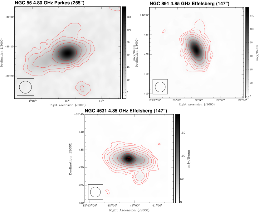
Figure 6: Single-dish maps of NGC 55 (top left), NGC 891 (top right) and NGC 4631 (bottom). Contours show the radio continuum emission at levels of $3\sigma\cdot 2^{n}$ ($n=0,1,2,\ldots$). The size of the primary beam is shown in the bottom left corner.

As part of our study we have obtained several additional radio continuum maps, which we present in this Appendix. We will make these maps publicly available (as well as all the other radio continuum maps in this paper); see Table 10 for the map properties. For 4 galaxies (NGC 55, 253, 891 and 4631) we have used single-dish maps, to correct for the missing zero-spacing flux where necessary. The Effelsberg maps of NGC 253 and 4631 were already presented in Heesen et al. (2009a) and Mora & Krause (2013), respectively, and the Effelsberg map of NGC 891 was already presented in Dumke (1997). We present these maps for completeness here again in Fig. 6. The $4.80$-GHz map of NGC 55 obtained with the 64-m Parkes telescope is so far unpublished and shown here also in Fig. 6.

Furthermore, we show in Fig. 7 two maps of NGC 4631 at $1.35$ and $1.65$ GHz observed with the VLA in D-configuration (R. Beck 2016, priv. comm.). The data were observed in August 1996, with 12 h on-source (ID: AG486) and reduced in standard fashion with AIPS. The maps have an angular resolution of 52 arcsec, so that we did not use them in the analysis, but they also show the halo of this galaxy very well. Lastly, we obtained maps of three further edge-on galaxies observed with the VLA (NGC 4157, 4217 and 4634), which we present in Fig. 8. We reduced the data as described in Section 2, but since we had only one frequency available and no spectral index map, we did not use them in the analysis. The maps of NGC 4157 and 4217 were created by re-reducing archive data (IDs AI23, AF85, AH457 and AS392 for NGC 4157 and ID AM573 for NGC 4217). The map of NGC 4634 was created by using so far unpublished data from the VLA (ID: AD538).

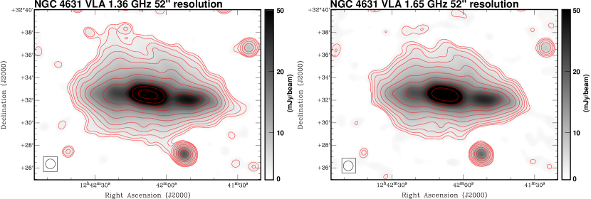
Figure 7: VLA maps of NGC 4631 at $1.37$ GHz (left) and $1.65$ GHz (right). Contours show the radio continuum emission at levels of $3\sigma\cdot 2^{n}$ ($n=0,1,2,\ldots$). The size of the synthesized beam is shown in the bottom left corner.

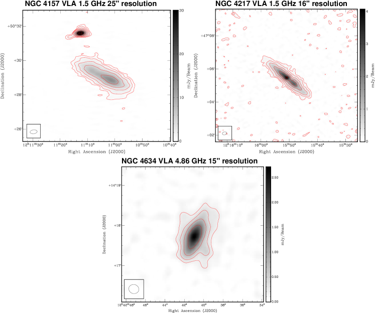
Figure 8: VLA maps of NGC 4157 (top left), NGC 4217 (top right) and NGC 4634 (bottom). Contours show the radio continuum emission at levels of $3\sigma\cdot 2^{n}$ ($n=0,1,2,\ldots$). The size of the synthesized beam is shown in the bottom left corner.

Appendix D Image atlas

In this appendix, we present maps and vertical profiles for individual galaxies. Each page shows results for one galaxy. The top row shows maps of the radio continuum emission at $L$ and $C$ band ($1.4$ and 5 GHz, except for NGC 5775 where instead of a $C$-band map we show an $X$-band map at $8.5$ GHz) and the thermal radio continuum emission at $5$ GHz (again, with the exception of NGC 5775, where we show the emission at $X$ band instead). The second row shows thermal fraction at $C$ band (again except for NGC 5775 where this is at $X$ band), the non-thermal radio spectral index between $L$ and $C$ band (for NGC 5775 between $L$ and $X$ band) and the corresponding error of the non-thermal radio spectral index. In the radio maps, contours show the radio continuum emission at levels of (3, 6, 12, 24, 48, 96) $\times\sigma$, where $\sigma$ is the rms noise of the map. For the thermal radio continuum map we use the same contours as of the radio continuum map of either $C$ or $X$ band. In the first and second row, the size of the synthesized beam is shown in the bottom left corner and all maps are rotated so that the major axis is horizontal. In panels (c)–(f), a mask has been applied (Section 2.3).

The third row shows vertical profiles of the non-thermal radio continuum intensities, vertical non-thermal intensity model profiles at one frequency and vertical profiles of the non-thermal radio spectral index. Panels (g) show exponential (solid) and Gaussian fits (dashed lines) to the data, panels (h) show model intensity profiles and panels (i) show radio spectral index profiles. The fourth row shows the reduced $\chi^{2}$ of the cosmic-ray transport model in the northern halo, in the southern halo and the vertical model profile of the magnetic field strength. In panels (j) and (k) contours show $\chi^{2}_{\rm int,min}+1$ for the intensity fitting (solid lines) and $\chi^{2}_{\rm spix,min}+1$ for spectral index fitting (dashed lines). The colour-scale shows the total reduced $\chi^{2}$ (sum of intensity and spectral index fitting). The best-fitting models (with uncertainties) lie in the intersection of the two contours and are marked by yellow stars. In panels (l), the grey-shaded area indicates the uncertainty of the magnetic field model.

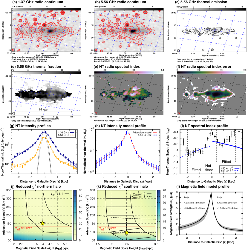
Figure 9: NGC 55. (a) radio continuum emission at $1.37$ GHz. (b) radio continuum emission at $5.56$ GHz. (c) thermal radio continuum emission at $5.56$ GHz. Contours in panels (a) and (b) are at (3, 6, 12, 24, 48 and 96) $\times\sigma$, where $\sigma$ is the rms map noise. In panel (c), the same contour levels as in (b) are used. (d) thermal fraction at $5.56$ GHz, where the grey-scale ranges from 0 to 40 per cent. (e) non-thermal radio spectral index between $1.37$ and $5.56$ GHz, where the colour scale ranges from $-1.2$ to $0$. (f) error of the non-thermal radio spectral index, where the colour scale ranges from 0 to $0.6$. Panels (a)–(f) are rotated so that the major axis ($PA=108\degr$) is horizontal and the synthesized beam is shown in the bottom left corner. (g) vertical non-thermal intensity profiles at both frequencies, where solid lines show two-component exponential fits and dashed lines two-component Gaussian fits. (h) normalized non-thermal vertical intensity model profile at $5.56$ GHz with best-fitting advection model. (i) vertical non-thermal radio spectral index profiles with best-fitting advection model. (j) reduced $\chi^{2}$ in the northern halo as function of advection speed and magnetic field scale height in the thick disc. (k) same as (j) but in the southern halo. The red lines in (j) and (k) show the escape velocity near the midplane. (l) vertical magnetic field model profile.                                                                                                                                   (The complete image atlas (12 images) is available in the online journal)

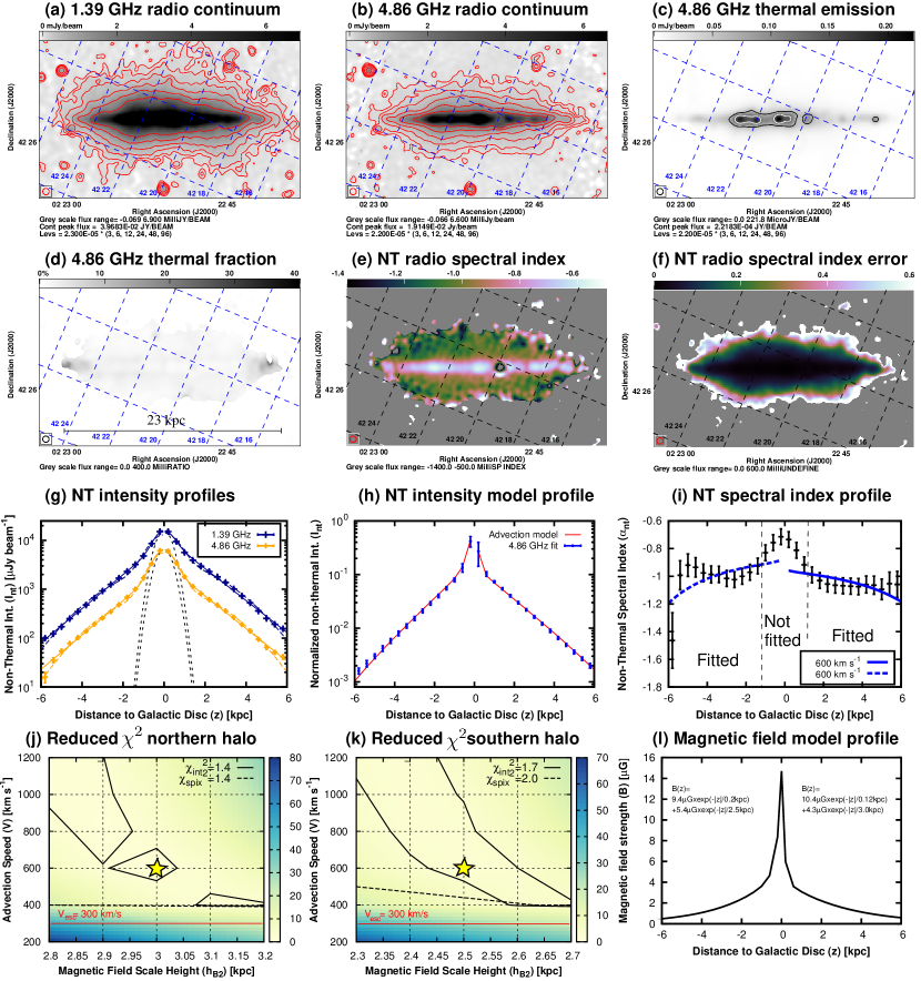
Figure 11: NGC 891. (a) radio continuum emission at $1.39$ GHz. (b) radio continuum emission at $4.86$ GHz. (c) thermal radio continuum emission at $4.86$ GHz. Contours in panels (a)–(c) are at (3, 6, 12, 24, 48 and 96) $\times\sigma$, where $\sigma$ is the rms map noise. In panel (c), the same contour levels as in (b) are used. (d) thermal fraction at $4.86$ GHz, where the grey-scale ranges from 0 to 40 per cent. (e) non-thermal radio spectral index between $1.39$ and $4.86$ GHz, where the colour scale ranges from $-1.4$ to $-0.5$. (f) error of the non-thermal radio spectral index, where the colour scale ranges from 0 to $0.6$. Panels (a)–(f) are rotated so that the major axis ($PA=23\degr$) is horizontal and the synthesized beam is shown in the bottom left corner. (g) vertical non-thermal intensity profiles at both frequencies, where solid lines show two-component exponential fits and dashed lines two-component Gaussian fits. (h) normalized vertical non-thermal intensity model profile at $4.86$ GHz with best-fitting advection model. (i) vertical non-thermal radio spectral index profile with best-fitting advection model. (j) reduced $\chi^{2}$ in the northern halo as function of advection speed and magnetic field scale height in the thick disc. (k) same as (j) but in the southern halo. The red lines in (j) and (k) show the escape velocity near the midplane. (l) vertical magnetic field model profile.

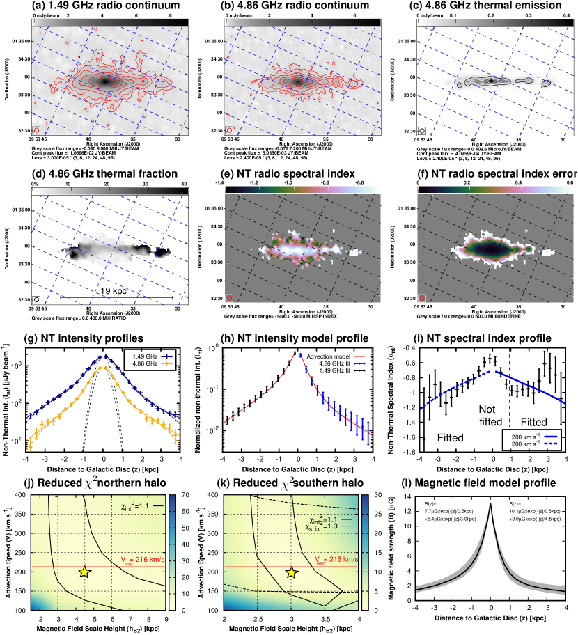
Figure 12: NGC 3044. (a) radio continuum emission at $1.49$ GHz. (b) radio continuum emission at $4.86$ GHz. (c) thermal radio continuum emission at $4.86$ GHz. Contours in panels (a)–(c) are at (3, 6, 12, 24, 48 and 96) $\times\sigma$, where $\sigma$ is the rms map noise. In panel (c), the same contour levels as in (b) are used. (d) thermal fraction at $4.86$ GHz, where the grey-scale ranges from 0 to 40 per cent. (e) non-thermal radio spectral index between $1.49$ and $4.86$ GHz, where the colour-scale ranges from $-1.4$ to $-0.5$. The spectral index error is $0.4$ in regions of low intensities and decreases to $0.1$ in regions of high intensities. (f) error of the non-thermal radio spectral index, where the colour scale ranges from 0 to $0.6$. Panels (a)–(f) are rotated so that the major axis ($PA=114\degr$) is horizontal and the synthesized beam is shown in the bottom left corner. (g) vertical non-thermal intensity profiles at both frequencies, where solid lines show two-component exponential fits and dashed lines two-component Gaussian fits. (h) normalized vertical non-thermal intensity model profile at $1.49$ and $4.86$ GHz with best-fitting advection model. (i) vertical non-thermal radio spectral index profile with best-fitting advection model. (j) reduced $\chi^{2}$ in the northern halo as function of advection speed and magnetic field scale height in the thick disc. (k) same as (j) but in the southern halo. The red lines in (j) and (k) show the escape velocity near the midplane. (l) vertical magnetic field model profile.

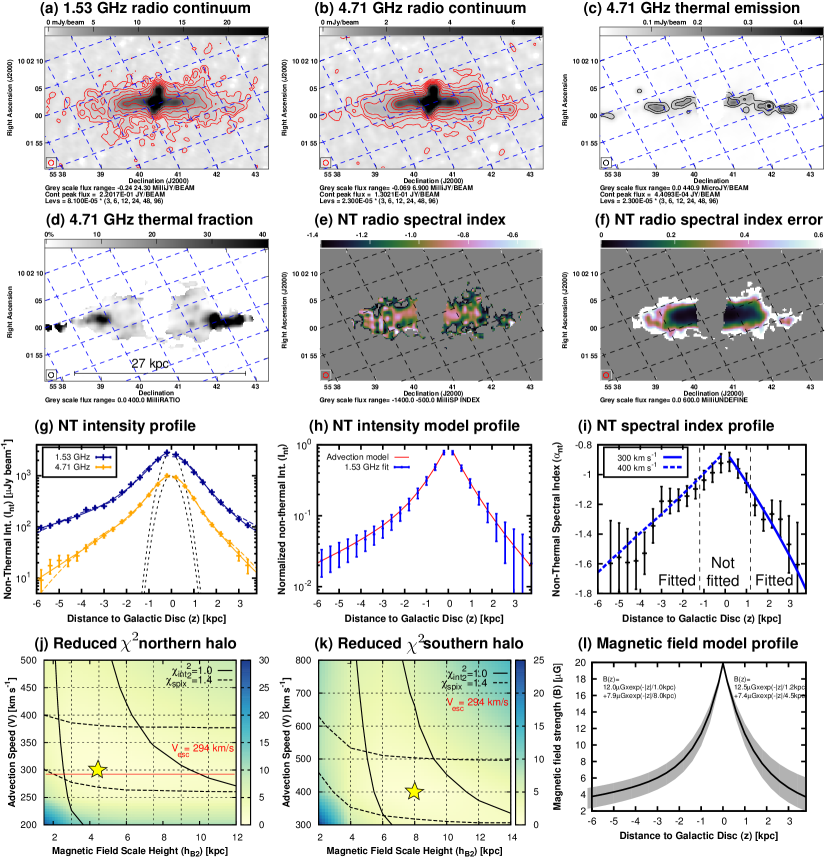
Figure 13: NGC 3079. (a) radio continuum emission at $1.53$ GHz. (b) radio continuum emission at $4.71$ GHz. (c) thermal radio continuum emission at $4.71$ GHz. Contours in panels (a) and (b) are at (3, 6, 12, 24, 48 and 96) $\times\sigma$, where $\sigma$ is the rms map noise. In panel (c), the same contour levels as in (b) are used. (d) thermal fraction at $4.71$ GHz, where the grey-scale ranges from 0 to 40 per cent. (e) non-thermal radio spectral index between $1.53$ and $4.71$ GHz, where the colour-scale ranges from $-1.4$ to $-0.5$. (f) error of the non-thermal radio spectral index, where the colour scale ranges from 0 to $0.6$. Panels (a)–(f) are rotated so that the major axis ($PA=167\degr$) is horizontal and the synthesized beam is shown in the bottom left corner. (g) vertical non-thermal intensity profiles at both frequencies, where solid lines show two-component exponential fits and dashed lines two-component Gaussian fits. (h) normalized vertical non-thermal intensity model profile at $1.53$ GHz with best-fitting advection model. (i) vertical non-thermal radio spectral index profile with best-fitting advection model. (j) reduced $\chi^{2}$ in the northern halo as function of advection speed and magnetic field scale height in the thick disc. (k) same as (j) but in the southern halo. The red line in (j) shows the escape velocity near the midplane. (l) vertical magnetic field model profile.

Figure 14: NGC 3628. (a) radio continuum emission at $1.49$ GHz. (b) radio continuum emission at $4.86$ GHz. (c) thermal radio continuum emission at $4.86$ GHz. Contours in panels (a)–(c) are at (3, 6, 12, 24, 48 and 96) $\times\sigma$, where $\sigma$ is the rms map noise. In panel (c) the rms noise of the map shown in (b) is used to ease the comparison. (d) thermal fraction at $4.86$ GHz, where the grey-scale ranges from 0 to 40 per cent. (e) non-thermal radio spectral index between $1.49$ and $4.86$ GHz, where the colour-scale ranges from $-1.4$ to $-0.5$. (f) error of the non-thermal radio spectral index, where the colour scale ranges from 0 to $0.6$. Panels (a)–(f) are rotated so that the major axis ($PA=105\degr$) is horizontal and the synthesized beam is shown in the bottom left corner. (g) vertical non-thermal intensity profiles at both frequencies, where solid lines show two-component exponential fits and dashed lines two-component Gaussian fits. (h) normalized vertical non-thermal intensity model profile at $1.49$ and $4.86$ GHz with best-fitting advection model. (i) vertical non-thermal radio spectral index profile with best-fitting advection model. (j) reduced $\chi^{2}$ in the northern halo as function of advection speed and magnetic field scale height in the thick disc. (k) same as (j) but in the southern halo. The red lines in (j) and (k) show the escape velocity near the midplane. (l) vertical magnetic field model profile.

Figure 15: NGC 4565. (a) radio continuum emission at $1.49$ GHz. (b) radio continuum emission at $4.86$ GHz. The increased noise level at the map edge is due to the correction for the primary beam attenuation of the VLA. (c) thermal radio continuum emission at $4.86$ GHz. Contours in panels (a) and (b) are at (3, 6, 12, 24, 48 and 96) $\times\sigma$, where $\sigma$ is the rms map noise. In panel (c), the same contour levels as in (b) are used. (d) thermal fraction at $4.86$ GHz, where the grey-scale ranges from 0 to 40 per cent. (e) non-thermal radio spectral index between $1.49$ and $4.86$ GHz, where the colour-scale ranges from $-1.4$ to $-0.5$. The spectral index error is $0.4$ in regions of low intensities and decreases to $0.1$ in regions of high intensities. (f) error of the non-thermal radio spectral index, where the colour scale ranges from 0 to $0.6$. Panels (a)–(f) are rotated so that the major axis ($PA=135\aas@@fstack{\circ}5$) is horizontal and the synthesized beam is shown in the bottom left corner. (g) vertical non-thermal intensity profiles at both frequencies, where solid lines show two-component exponential fits and dashed lines two-component Gaussian fits. (h) normalized vertical non-thermal intensity model profile at $1.49$ GHz with best-fitting advection model. (i) vertical non-thermal radio spectral index profile with best-fitting advection model. (j) reduced $\chi^{2}$ in the northern halo as function of advection speed and magnetic field scale height in the thick disc. (k) same as (j) but in the southern halo. The red lines in (j) and (k) show the escape velocity near the midplane. (l) vertical magnetic field model profile.

Figure 16: NGC 4631. (a) radio continuum emission at $1.37$ GHz. (b) radio continuum emission at $4.86$ GHz. The high noise level near the edge of the map stems from the correction for the primary beam attenuation of the VLA. (c) thermal radio continuum emission at $4.86$ GHz. Contours in panels (a)–(c) are at (3, 6, 12, 24, 48 and 96) $\times\sigma$, where $\sigma$ is the rms map noise. In panel (c), the same contour levels as in (b) are used to ease the comparison. (d) thermal fraction at $4.86$ GHz, where the grey-scale ranges from 0 to 40 per cent. (e) non-thermal radio spectral index between $1.37$ and $4.86$ GHz, where the colour scale ranges from $-1.4$ to $-0.5$. (f) error of the non-thermal radio spectral index, where the colour scale ranges from 0 to $0.6$. Panels (a)–(f) are rotated so that the major axis ($PA=86\degr$) is horizontal and the synthesized beam is shown in the bottom left corner. (g) vertical non-thermal intensity profiles at both frequencies, where solid lines show two-component exponential fits and dashed lines two-component Gaussian fits. (h) normalized vertical non-thermal intensity model profile at $1.37$ GHz with best-fitting advection model. (i) vertical non-thermal radio spectral index profile with best-fitting advection model. (j) reduced $\chi^{2}$ in the northern halo as function of advection speed and magnetic field scale height in the thick disc. (k) same as (j) but in the southern halo. The red line in (k) shows the escape velocity near the midplane. (l) vertical magnetic field model profile.

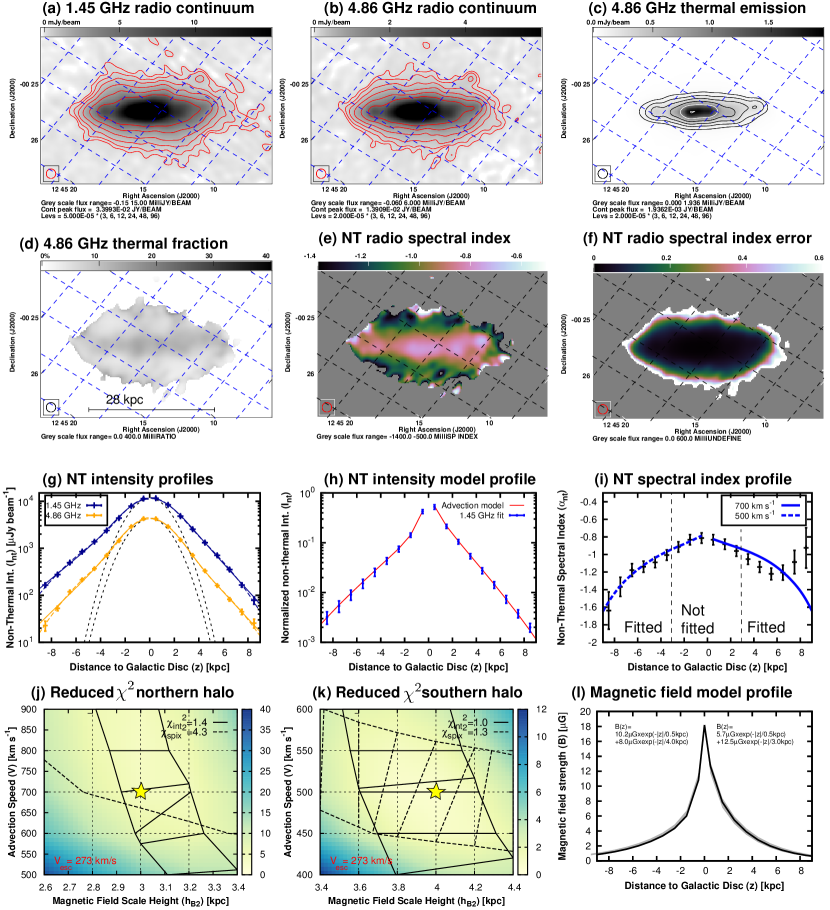
Figure 17: NGC 4666. (a) radio continuum emission at $1.45$ GHz. (b) radio continuum emission at $4.86$ GHz. (c) thermal radio continuum emission at $4.86$ GHz. Contours in panels (a) and (b) are at (3, 6, 12, 24, 48 and 96) $\times\sigma$, where $\sigma$ is the rms map noise. In panel (c), the same contour levels as in (b) are used. (d) thermal fraction at $4.86$ GHz, where the grey scale ranges from 0 to 40 per cent. (e) non-thermal radio spectral index between $1.45$ and $4.86$ GHz, where the colour scale ranges from $-1.4$ to $-0.5$. (f) error of the non-thermal radio spectral index, where the colour scale ranges from 0 to $0.6$. Panels (a)–(f) are rotated so that the major axis ($PA=40\degr$) is horizontal and the synthesized beam is shown in the bottom left corner. (g) vertical non-thermal intensity profiles at both frequencies, where solid lines show two-component exponential fits and dashed lines two-component Gaussian fits. (h) normalized vertical non-thermal intensity model profile at $1.45$ GHz with best-fitting advection model. (i) vertical non-thermal radio spectral index profile with best-fitting advection model. (j) reduced $\chi^{2}$ in the northern halo as function of advection speed and magnetic field scale height in the thick disc. (k) same as (j) but in the southern halo. (l) vertical magnetic field model profile.

Figure 18: NGC 5775. (a) radio continuum emission at $1.49$ GHz. (b) radio continuum emission at $8.46$ GHz. (c) thermal radio continuum emission at $8.46$ GHz. Contours in panels (a) and (b) are at (3, 6, 12, 24, 48 and 96) $\times\sigma$, where $\sigma$ is the rms map noise. In panel (c), the same contour levels as in (b) are used. (d) thermal fraction at $8.46$ GHz, where the grey-scale ranges from 0 to 40 per cent. (e) non-thermal radio spectral index between $1.49$ and $8.46$ GHz, where the colour-scale ranges from $-1.4$ to $-0.5$. (f) error of the non-thermal radio spectral index, where the colour scale ranges from 0 to $0.6$. Panels (a)–(f) are rotated so that the major axis ($PA=145\degr$) is horizontal and the synthesized beam is shown in the bottom left corner. (g) vertical non-thermal intensity profiles at both frequencies, where solid lines show two-component exponential fits and dashed lines two-component Gaussian fits. (h) normalized vertical non-thermal intensity model profile at $1.49$ GHz with best-fitting advection model. (i) vertical non-thermal radio spectral index profile with best-fitting advection model. (j) reduced $\chi^{2}$ in the northern halo as function of advection speed and magnetic field scale height in the thick disc. (k) same as (j) but in the southern halo. (l) vertical magnetic field model profile.

Figure 19: NGC 7090. (a) radio continuum emission at $1.38$ GHz. (b) radio continuum emission at $4.68$ GHz. (c) thermal radio continuum emission at $4.68$ GHz. Contours in panels (a) and (b) are at (3, 6, 12, 24, 48 and 96) $\times\sigma$, where $\sigma$ is the rms map noise. In panel (c), the same contour levels as in (b) are used. (d) thermal fraction at $4.68$ GHz, where the grey-scale ranges from 0 to 40 per cent. (e) non-thermal radio spectral index between $1.38$ and $4.68$ GHz, where the colour-scale ranges from $-1.4$ to $-0.5$. (f) error of the non-thermal radio spectral index, where the colour scale ranges from 0 to $0.6$. Panels (a)–(f) are rotated so that the major axis ($PA=128\degr$) is horizontal and the synthesized beam is shown in the bottom left corner. (g) vertical non-thermal intensity profiles at both frequencies, where solid lines show two-component exponential fits and dashed lines two-component Gaussian fits. (h) normalized vertical non-thermal intensity model profile at $1.38$ GHz with best-fitting advection model. (i) vertical non-thermal radio spectral index profile with best-fitting advection model. (j) reduced $\chi^{2}$ in the northern halo as function of advection speed and magnetic field scale height in the thick disc. (k) same as (j) but in the southern halo. The red lines (j) and (k) show the escape velocity near the midplane. (l) vertical magnetic field model profile.

Figure 20: NGC 7462. (a) radio continuum emission at $1.38$ GHz. (b) radio continuum emission at $4.68$ GHz. (c) thermal radio continuum emission at $4.68$ GHz. Contours in panels (a) and (b) are at (3, 6, 12, 24, 48 and 96) $\times\sigma$, where $\sigma$ is the rms map noise. In panel (c), the same contour levels as in (b) are used. (d) thermal fraction at $4.68$ GHz, where the grey-scale ranges from 0 to 40 per cent. (e) non-thermal radio spectral index between $1.38$ and $4.68$ GHz, where the colour-scale ranges from $-1.8$ to $-0.5$. The spectral index error is $0.4$ in regions of low intensities and decreases to $0.1$ in regions of high intensities. (f) error of the non-thermal radio spectral index, where the colour scale ranges from 0 to $0.6$. Panels (a)–(f) are rotated so that the major axis ($PA=73\degr$) is horizontal and the synthesized beam is shown in the bottom left corner. (g) vertical non-thermal intensity profiles at both frequencies, where solid lines show two-component exponential fits and dashed lines two-component Gaussian fits. (h) normalized vertical non-thermal intensity model profile at $1.38$ GHz with best-fitting diffusion model. (i) vertical non-thermal radio spectral index profile with best-fitting diffusion model. (j) reduced $\chi^{2}$ in the northern halo as function of diffusion coefficient and magnetic field scale height in the thick disc. (k) same as (j) but in the southern halo. (l) vertical model magnetic field profile.

References

- Adebahr et al. (2013) Adebahr B., Krause M., Klein U., Weżgowiec M., Bomans D. J., Dettmar R.-J., 2013, A&A, 555, A23
- Arribas et al. (2014) Arribas S., Colina L., Bellocchi E., Maiolino R., Villar-Martín M., 2014, A&A, 568, A14
- Baars et al. (1977) Baars J. W. M., Genzel R., Pauliny-Toth I. I. K., Witzel A., 1977, A&A, 61, 99
- Bagetakos et al. (2011) Bagetakos I., Brinks E., Walter F., de Blok W. J. G., Usero A., Leroy A. K., Rich J. W., Kennicutt Jr. R. C., 2011, AJ, 141, 23
- Basu et al. (2015) Basu A., Beck R., Schmidt P., Roy S., 2015, MNRAS, 449, 3879
- Bauer et al. (2008) Bauer M., Pietsch W., Trinchieri G., Breitschwerdt D., Ehle M., Freyberg M. J., Read A. M., 2008, A&A, 489, 1029
- Beck (2016) Beck R., 2016, A&ARv, 24, 4
- Beck & Krause (2005) Beck R., Krause M., 2005, Astron. Nachr., 326, 414
- Becker et al. (1991) Becker R. H., White R. L., Edwards A. L., 1991, ApJS, 75, 1
- Bell (1978) Bell A. R., 1978, MNRAS, 182, 147
- Bendo et al. (2012) Bendo G. J., Galliano F., Madden S. C., 2012, MNRAS, 423, 197
- Berkhuijsen et al. (2013) Berkhuijsen E. M., Beck R., Tabatabaei F. S., 2013, MNRAS, 435, 1598
- Braun et al. (2007) Braun R., Oosterloo T. A., Morganti R., Klein U., Beck R., 2007, A&A, 461, 455
- Breitschwerdt et al. (1991) Breitschwerdt D., McKenzie J. F., Völk H. J., 1991, A&A, 245, 79
- Breitschwerdt et al. (1993) Breitschwerdt D., McKenzie J. F., Völk H. J., 1993, A&A, 269, 54
- Breitschwerdt et al. (2012) Breitschwerdt D., de Avillez M. A., Baumgartner V., Dogiel V. A., 2012, in de Avillez M. A., ed., EAS Publications Series Vol. 56, EAS Publications Series. pp 333–342 (arXiv:0905.0431), doi:10.1051/eas/1256055
- Carilli et al. (1992) Carilli C. L., Holdaway M. A., Ho P. T. P., de Pree C. G., 1992, ApJ, 399, L59
- Carretti et al. (2010) Carretti E., Haverkorn M., McConnell D., Bernardi G., McClure-Griffiths N. M., Cortiglioni S., Poppi S., 2010, MNRAS, 405, 1670
- Cecil et al. (2001) Cecil G., Bland-Hawthorn J., Veilleux S., Filippenko A. V., 2001, ApJ, 555, 338
- Cecil et al. (2002) Cecil G., Bland-Hawthorn J., Veilleux S., 2002, ApJ, 576, 745
- Chyży et al. (2016) Chyży K. T., Drzazga R. T., Beck R., Urbanik M., Heesen V., Bomans D. J., 2016, ApJ, 819, 39
- Colbert et al. (1996) Colbert E. J. M., Baum S. A., Gallimore J. F., O’Dea C. P., Christensen J. A., 1996, ApJ, 467, 551
- Collins et al. (2000) Collins J. A., Rand R. J., Duric N., Walterbos R. A. M., 2000, ApJ, 536, 645
- Condon (1992) Condon J. J., 1992, ARA&A, 30, 575
- Condon et al. (1996) Condon J. J., Helou G., Sanders D. B., Soifer B. T., 1996, ApJS, 103, 81
- Condon et al. (2002) Condon J. J., Cotton W. D., Broderick J. J., 2002, AJ, 124, 675
- Dahlem et al. (1994) Dahlem M., Dettmar R.-J., Hummel E., 1994, A&A, 290, 384
- Dahlem et al. (1997) Dahlem M., Petr M. G., Lehnert M. D., Heckman T. M., Ehle M., 1997, A&A, 320, 731
- Dahlem et al. (2005) Dahlem M., Ehle M., Ryder S. D., Vlajić M., Haynes R. F., 2005, A&A, 432, 475
- Dale & Helou (2002) Dale D. A., Helou G., 2002, ApJ, 576, 159
- Dale et al. (2009) Dale D. A., et al., 2009, ApJ, 703, 517
- Dorfi & Breitschwerdt (2012) Dorfi E. A., Breitschwerdt D., 2012, A&A, 540, A77
- Draine (2011) Draine B. T., 2011, Physics of the Interstellar and Intergalactic Medium. Princeton University Press, Princeton, NJ
- Dumke (1997) Dumke M., 1997, PhD thesis, University of Bonn
- Dumke & Krause (1998) Dumke M., Krause M., 1998, in Breitschwerdt D., Freyberg M. J., Trümper J., eds, Lecture Notes in Physics, Berlin Springer Verlag Vol. 506, IAU Colloq. 166: The Local Bubble and Beyond. p. 555
- Dumke et al. (1995) Dumke M., Krause M., Wielebinski R., Klein U., 1995, A&A, 302, 691
- Duric et al. (1998) Duric N., Irwin J., Bloemen H., 1998, A&A, 331, 428
- Engelbracht et al. (2008) Engelbracht C. W., Rieke G. H., Gordon K. D., Smith J.-D. T., Werner M. W., Moustakas J., Willmer C. N. A., Vanzi L., 2008, ApJ, 678, 804
- Everett et al. (2008) Everett J. E., Zweibel E. G., Benjamin R. A., McCammon D., Rocks L., Gallagher III J. S., 2008, ApJ, 674, 258
- Ferrière (2001) Ferrière K. M., 2001, Rev. Modern Phys., 73, 1031
- Fletcher (2010) Fletcher A., 2010, in Kothes R., Landecker T. L., Willis A. G., eds, Astronomical Society of the Pacific Conference Series Vol. 438, The Dynamic Interstellar Medium: A Celebration of the Canadian Galactic Plane Survey. p. 197 (arXiv:1104.2427)
- Gil de Paz et al. (2007) Gil de Paz A., et al., 2007, ApJS, 173, 185
- Golla & Hummel (1994) Golla G., Hummel E., 1994, A&A, 284, 777
- Gregory & Condon (1991) Gregory P. C., Condon J. J., 1991, ApJS, 75, 1011
- Griffith & Wright (1993) Griffith M. R., Wright A. E., 1993, AJ, 105, 1666
- Griffith et al. (1995) Griffith M. R., Wright A. E., Burke B. F., Ekers R. D., 1995, ApJS, 97, 347
- Haverkorn & Heesen (2012) Haverkorn M., Heesen V., 2012, Space Sci. Rev., 166, 133
- Haynes et al. (1979) Haynes M. P., Giovanelli R., Roberts M. S., 1979, ApJ, 229, 83
- Heald (2012) Heald G. H., 2012, ApJ, 754, L35
- Heckman & Borthakur (2016) Heckman T. M., Borthakur S., 2016, ApJ, 822, 9
- Heckman et al. (2000) Heckman T. M., Lehnert M. D., Strickland D. K., Armus L., 2000, ApJS, 129, 493
- Heckman et al. (2015) Heckman T. M., Alexandroff R. M., Borthakur S., Overzier R., Leitherer C., 2015, ApJ, 809, 147
- Heesen et al. (2009a) Heesen V., Beck R., Krause M., Dettmar R.-J., 2009a, A&A, 494, 563
- Heesen et al. (2009b) Heesen V., Krause M., Beck R., Dettmar R.-J., 2009b, A&A, 506, 1123
- Heesen et al. (2011) Heesen V., Beck R., Krause M., Dettmar R.-J., 2011, A&A, 535, A79
- Heesen et al. (2014) Heesen V., Brinks E., Leroy A. K., Heald G., Braun R., Bigiel F., Beck R., 2014, AJ, 147, 103
- Heesen et al. (2015) Heesen V., et al., 2015, MNRAS, 447, L1
- Heesen et al. (2016) Heesen V., Dettmar R.-J., Krause M., Beck R., Stein Y., 2016, MNRAS, 458, 332
- Heesen et al. (2018) Heesen V., et al., 2018, MNRAS, 474, 5049
- Henriksen & Irwin (2016) Henriksen R. N., Irwin J. A., 2016, MNRAS, 458, 4210
- Ho et al. (1997) Ho L. C., Filippenko A. V., Sargent W. L. W., 1997, ApJS, 112, 315
- Hodges-Kluck & Bregman (2013) Hodges-Kluck E. J., Bregman J. N., 2013, ApJ, 762, 12
- Hummel et al. (1988) Hummel E., Lesch H., Wielebinski R., Schlickeiser R., 1988, A&A, 197, L29
- Hunter et al. (2012) Hunter D. A., et al., 2012, AJ, 144, 134
- Irwin et al. (1999) Irwin J. A., English J., Sorathia B., 1999, AJ, 117, 2102
- Irwin et al. (2011) Irwin J. A., et al., 2011, MNRAS, 410, 1423
- Irwin et al. (2012) Irwin J., et al., 2012, AJ, 144, 43
- Irwin et al. (2013) Irwin J. A., Brar R. S., Saikia D. J., Henriksen R. N., 2013, MNRAS, 433, 2958
- James et al. (2004) James P. A., et al., 2004, A&A, 414, 23
- Karachentsev et al. (2003) Karachentsev I. D., et al., 2003, A&A, 404, 93
- Karachentsev et al. (2013) Karachentsev I. D., Makarov D. I., Kaisina E. I., 2013, AJ, 145, 101
- Kennicutt & Evans (2012) Kennicutt R. C., Evans N. J., 2012, ARA&A, 50, 531
- Kennicutt et al. (2008) Kennicutt Jr. R. C., Lee J. C., Funes José G. S. J., Sakai S., Akiyama S., 2008, ApJS, 178, 247
- Kettenis et al. (2006) Kettenis M., van Langevelde H. J., Reynolds C., Cotton B., 2006, in Gabriel C., Arviset C., Ponz D., Enrique S., eds, Astronomical Society of the Pacific Conference Series Vol. 351, Astronomical Data Analysis Software and Systems XV. p. 497
- Krause (2009) Krause M., 2009, Rev. Mex. Astron. Astrofis., 36, 25
- Krause (2015) Krause M., 2015, Highlights of Astronomy, 16, 399
- Krause et al. (2006) Krause M., Wielebinski R., Dumke M., 2006, A&A, 448, 133
- Krause et al. (2017) Krause M., et al., 2017, preprint, (arXiv:1712.03780)
- Lee & Irwin (1997) Lee S.-W., Irwin J. A., 1997, ApJ, 490, 247
- Li et al. (2016) Li J.-T., et al., 2016, MNRAS, 456, 1723
- Lisenfeld & Völk (2000) Lisenfeld U., Völk H. J., 2000, A&A, 354, 423
- Longair (2011) Longair M. S., 2011, High Energy Astrophysics. Cambridge University Press, Cambridge, UK
- Mac Low & Ferrara (1999) Mac Low M.-M., Ferrara A., 1999, ApJ, 513, 142
- Makarov et al. (2014) Makarov D., Prugniel P., Terekhova N., Courtois H., Vauglin I., 2014, A&A, 570, A13
- Mao et al. (2015) Mao S. A., Zweibel E., Fletcher A., Ott J., Tabatabaei F., 2015, ApJ, 800, 92
- Martin (2005) Martin C. L., 2005, ApJ, 621, 227
- McMullin et al. (2007) McMullin J. P., Waters B., Schiebel D., Young W., Golap K., 2007, in Shaw R. A., Hill F., Bell D. J., eds, ASP Conf. Ser. Vol. 376, Astronomical Data Analysis Software and Systems XVI. Astron. Soc. Pac., San Francisco, p. 127.
- Middelberg et al. (2007) Middelberg E., Agudo I., Roy A. L., Krichbaum T. P., 2007, MNRAS, 377, 731
- Mora & Krause (2013) Mora S. C., Krause M., 2013, A&A, 560, A42
- Moshir et al. (1990) Moshir M., et al., 1990, in Bulletin of the American Astronomical Society. p. 1325
- Moustakas & Kennicutt (2006) Moustakas J., Kennicutt Jr. R. C., 2006, ApJS, 164, 81
- Mulcahy et al. (2014) Mulcahy D. D., et al., 2014, A&A, 568, A74
- Mulcahy et al. (2016) Mulcahy D. D., Fletcher A., Beck R., Mitra D., Scaife A. M. M., 2016, A&A, 592, A123
- Mulcahy et al. (2017) Mulcahy D. D., Beck R., Heald G. H., 2017, A&A, 600, A6
- Murray et al. (2005) Murray N., Quataert E., Thompson T. A., 2005, ApJ, 618, 569
- Niklas & Beck (1997) Niklas S., Beck R., 1997, A&A, 320, 54
- Niklas et al. (1997) Niklas S., Klein U., Wielebinski R., 1997, A&A, 322, 19
- Oosterloo et al. (2007) Oosterloo T., Fraternali F., Sancisi R., 2007, AJ, 134, 1019
- Parker (1992) Parker E. N., 1992, ApJ, 401, 137
- Pence (1981) Pence W. D., 1981, ApJ, 247, 473
- Perley & Butler (2013) Perley R. A., Butler B. J., 2013, ApJS, 204, 19
- Pietrzyński et al. (2006) Pietrzyński G., et al., 2006, AJ, 132, 2556
- Ptuskin et al. (1997) Ptuskin V. S., Voelk H. J., Zirakashvili V. N., Breitschwerdt D., 1997, A&A, 321, 434
- Rand et al. (2011) Rand R. J., Wood K., Benjamin R. A., Meidt S. E., 2011, ApJ, 728, 163
- Rau & Cornwell (2011) Rau U., Cornwell T. J., 2011, A&A, 532, A71
- Recchia et al. (2016a) Recchia S., Blasi P., Morlino G., 2016a, MNRAS, 462, L88
- Recchia et al. (2016b) Recchia S., Blasi P., Morlino G., 2016b, MNRAS, 462, 4227
- Reuter et al. (1991) Reuter H.-P., Krause M., Wielebinski R., Lesch H., 1991, A&A, 248, 12
- Rice et al. (1988) Rice W., Lonsdale C. J., Soifer B. T., Neugebauer G., Kopan E. L., Lloyd L. A., de Jong T., Habing H. J., 1988, ApJS, 68, 91
- Rieger et al. (2013) Rieger F. M., de Oña-Wilhelmi E., Aharonian F. A., 2013, Frontiers of Physics, 8, 714
- Robitaille et al. (2007) Robitaille T. P., Rossa J., Bomans D. J., van der Marel R. P., 2007, A&A, 464, 541
- Rossa & Dettmar (2003a) Rossa J., Dettmar R.-J., 2003a, A&A, 406, 493
- Rossa & Dettmar (2003b) Rossa J., Dettmar R.-J., 2003b, A&A, 406, 505
- Rupen et al. (1987) Rupen M. P., van Gorkom J. H., Knapp G. R., Gunn J. E., Schneider D. P., 1987, AJ, 94, 61
- Rupke et al. (2005) Rupke D. S., Veilleux S., Sanders D. B., 2005, ApJS, 160, 115
- Salem & Bryan (2014) Salem M., Bryan G. L., 2014, MNRAS, 437, 3312
- Samui et al. (2010) Samui S., Subramanian K., Srianand R., 2010, MNRAS, 402, 2778
- Sanders et al. (2003) Sanders D. B., Mazzarella J. M., Kim D.-C., Surace J. A., Soifer B. T., 2003, AJ, 126, 1607
- Sault et al. (1995) Sault R. J., Teuben P. J., Wright M. C. H., 1995, in Shaw R. A., Payne H. E., Hayes J. J. E., eds, ASP Conf. Ser. Vol. 77, Astronomical Data Analysis Software and Systems IV. Astron. Soc. Pac., San Francisco, p. 433.
- Sault et al. (1996) Sault R. J., Staveley-Smith L., Brouw W. N., 1996, A&AS, 120, 375
- Shafi et al. (2015) Shafi N., Oosterloo T. A., Morganti R., Colafrancesco S., Booth R., 2015, MNRAS, 454, 1404
- Sofue et al. (1994) Sofue Y., Wakamatsu K.-I., Malin D. F., 1994, AJ, 108, 2102
- Soida et al. (2011) Soida M., Krause M., Dettmar R.-J., Urbanik M., 2011, A&A, 531, A127
- Soifer et al. (1989) Soifer B. T., Boehmer L., Neugebauer G., Sanders D. B., 1989, AJ, 98, 766
- Stil et al. (2009) Stil J. M., Krause M., Beck R., Taylor A. R., 2009, ApJ, 693, 1392
- Strickland et al. (2004) Strickland D. K., Heckman T. M., Colbert E. J. M., Hoopes C. G., Weaver K. A., 2004, ApJS, 151, 193
- Strong et al. (2007) Strong A. W., Moskalenko I. V., Ptuskin V. S., 2007, Annu. Rev. Nucl. Part. Sci., 57, 285
- Sukumar & Allen (1991) Sukumar S., Allen R. J., 1991, ApJ, 382, 100
- Tabatabaei et al. (2013a) Tabatabaei F. S., et al., 2013a, A&A, 552, A19
- Tabatabaei et al. (2013b) Tabatabaei F. S., Berkhuijsen E. M., Frick P., Beck R., Schinnerer E., 2013b, A&A, 557, A129
- Tabatabaei et al. (2017) Tabatabaei F. S., et al., 2017, ApJ, 836, 185
- Tüllmann et al. (2000) Tüllmann R., Dettmar R.-J., Soida M., Urbanik M., Rossa J., 2000, A&A, 364, L36
- Tully & Fisher (1988) Tully R. B., Fisher J. R., 1988, Catalog of Nearby Galaxies
- Veilleux et al. (1995) Veilleux S., Kim D.-C., Sanders D. B., Mazzarella J. M., Soifer B. T., 1995, ApJS, 98, 171
- Voigtländer et al. (2013) Voigtländer P., Kamphuis P., Marcelin M., Bomans D. J., Dettmar R.-J., 2013, A&A, 554, A133
- Vollmer et al. (2016) Vollmer B., Nehlig F., Ibata R., 2016, A&A, 586, A98
- Wells (1997) Wells B. S., 1997, Publ. Astron. Soc. Australia, 14, 292
- Westmeier et al. (2013) Westmeier T., Koribalski B. S., Braun R., 2013, MNRAS, 434, 3511
- Westmoquette et al. (2011) Westmoquette M. S., Smith L. J., Gallagher III J. S., 2011, MNRAS, 414, 3719
- White & Becker (1992) White R. L., Becker R. H., 1992, ApJS, 79, 331
- Wiegert et al. (2015) Wiegert T., et al., 2015, AJ, 150, 81
- Wilson et al. (2011) Wilson W. E., et al., 2011, MNRAS, 416, 832
- Wright et al. (1994) Wright A. E., Griffith M. R., Burke B. F., Ekers R. D., 1994, ApJS, 91, 111
- Yoast-Hull et al. (2013) Yoast-Hull T. M., Everett J. E., Gallagher III J. S., Zweibel E. G., 2013, ApJ, 768, 53
- Young et al. (1996) Young J. S., Allen L., Kenney J. D. P., Lesser A., Rownd B., 1996, AJ, 112, 1903
- Zschaechner et al. (2012) Zschaechner L. K., Rand R. J., Heald G. H., Gentile G., Józsa G., 2012, ApJ, 760, 37
- Zschaechner et al. (2015) Zschaechner L. K., Rand R. J., Walterbos R., 2015, ApJ, 799, 61
- van Haarlem et al. (2013) van Haarlem M. P., et al., 2013, A&A, 556, A2