Abstract

For the search for electroweak particles in the Minimal Supersymmetric Standard Model (MSSM) as well as for future precision analyses of these particles an accurate knowledge of their production and decay properties is mandatory. We review the evaluation of the cross sections for the chargino, neutralino and scalar lepton production at $e^{+}e^{-}$ colliders in the MSSM with complex parameters (cMSSM). The evaluation is based on a full one-loop calculation of the various production mechanisms, including soft and hard photon radiation. The dependence of the chargino/neutralino/slepton cross sections on the relevant cMSSM parameters is analyzed numerically. We find sizable contributions to many production cross sections. They amount roughly $\pm 15\,\%$ of the tree-level results, but can go up to $\pm 40\,\%$ or higher in extreme cases. Also the complex phase dependence of the one-loop corrections was found non-negligible. The full one-loop contributions are thus crucial for physics analyses at a future linear $e^{+}e^{-}$ collider such as the ILC or CLIC.

1 Introduction

One of the most important tasks at the LHC is to search for physics beyond the Standard Model (SM), where the Minimal Supersymmetric Standard Model (MSSM) [2, 3, 4] is one of the leading candidates. Supersymmetry (SUSY) predicts two scalar partners for all SM fermions as well as fermionic partners to all SM bosons. In particular two scalar quarks or scalar leptons are predicted for each SM quark or lepton. Concerning the Higgs-boson sector, contrary to the case of the SM, in the MSSM two Higgs doublets are required. This results in five physical Higgs bosons instead of the single Higgs boson in the SM. These are the light and heavy ${{\cal CP}}$-even Higgs bosons, $h$ and $H$, the ${{\cal CP}}$-odd Higgs boson, $A$, and the charged Higgs bosons, $H^{\pm}$. At tree-level the Higgs sector is described by the mass of the charged Higgs boson, $M_{H^{\pm}}$ and the ratio of the two vacuum expectation values, $\tan\beta\equiv t_{\beta}:=v_{2}/v_{1}$. Higher-order corrections are crucial to yield reliable predictions in the MSSM Higgs-boson sector, see Refs. [5, 6, 7] for reviews. The neutral SUSY partners of the (neutral) Higgs and electroweak gauge bosons are the four neutralinos, $\tilde{\chi}_{1,2,3,4}^{0}$. The corresponding charged SUSY partners are the charginos, $\tilde{\chi}_{1,2}^{\pm}$.

If SUSY is realized in nature and the scalar quarks and/or the gluino are in the kinematic reach of the LHC, it is expected that these strongly interacting particles are copiously produced eventually. On the other hand, SUSY particles that interact only via the electroweak force, i.e.  the charginos, neutralinos and sleptons, have a much smaller production cross section at the LHC. Correspondingly, the LHC discovery potential as well as the current experimental bounds are substantially weaker.

At a (future) $e^{+}e^{-}$ collider charginos, neutralinos and sleptons, depending on their masses and the available center-of-mass energy, could be produced and analyzed in detail, see e.g. Ref. [8]. Corresponding studies can be found for the ILC in Refs. [9, 10, 11, 12] and for CLIC in Refs. [13, 12]. (Results on the combination of LHC and ILC results can be found in Ref. [14].) Such precision studies will be crucial to determine the nature of those particles and the underlying SUSY parameters.

In order to yield a sufficient accuracy, one-loop corrections to the various chargino/neutralino/slepton production and decay modes have to be considered. Full one-loop calculations in the cMSSM for various chargino/neutralino/slepton decays in the cMSSM have been presented over the last years [15, 16, 17, 18]. One-loop corrections for their production from the decay of Higgs bosons (at the LHC or ILC/CLIC) can be found in Refs. [19, 20]. Here we review the recent calculations of chargino/neutralino production at $e^{+}e^{-}$ colliders [21] and give a preview of the slepton production at $e^{+}e^{-}$ colliders [22]. The following channels are considered:

$$\sigma(e^{+}e^{-}\to\tilde{\chi}_{c}^{\pm}\tilde{\chi}_{c^{\prime}}^{\mp})\qquad(c,c^{\prime}=1,2)\,,$$ (1)

$$\sigma(e^{+}e^{-}\to\tilde{\chi}_{n}^{0}\tilde{\chi}_{n^{\prime}}^{0})\qquad(n,n^{\prime}=1,2,3,4)\,,$$ (2)

$$\sigma(e^{+}e^{-}\to\mathrm{\tilde{e}}^{\pm}_{gs}\mathrm{\tilde{e}}^{\mp}_{gs^{\prime}})\qquad(s,s^{\prime}=1,2)\,,$$ (3)

$$\sigma(e^{+}e^{-}\to\tilde{\nu}_{g}\tilde{\nu}_{g})\,,$$ (4)

with $\mathrm{\tilde{e}}_{g}=\{\tilde{e},\tilde{\mu},\tilde{\tau}\}$, $\tilde{\nu}_{g}=\{\tilde{\nu}_{e},\tilde{\nu}_{\mu},\tilde{\nu}_{\tau}\}$, and the generation index $g=1,2,3$. Our evaluation of the four channels (1) – (4) is based on a full one-loop calculation, i.e. including electroweak (EW) corrections, as well as soft and hard QED radiation. The renormalization scheme employed is the same one as for the decay of charginos/neutralinos/sleptons [15, 16, 17, 18]. Consequently, the predictions for the production and decay can be used together in a consistent manner.

2 The production processes at one-loop

Here we briefly review the contributing loop diagrams to the processes (1) – (4). The diagrams and corresponding amplitudes have been obtained with FeynArts [23], using the MSSM model file (including the MSSM counterterms) of Ref. [24]. The further evaluation has been performed with FormCalc and LoopTools [25]. The specific versions of the codes used can be found in Refs. [21, 22]. All relevant details about the various sectors of the cMSSM and their renormalization as well as on the cancellation of the UV, IR and collinear divergences can also be found in Refs. [21, 22], see also the descriptions given in Refs. [19, 20, 24, 26, 27, 28, 15, 16, 17, 18, 29, 30].

2.1 Contributing diagrams for chargino/neutralino production

Figure 1: Generic tree, self-energy, vertex, box, and counterterm diagrams for the process $e^{+}e^{-}\to\tilde{\chi}_{c}^{\pm}\tilde{\chi}_{c^{\prime}}^{\mp}$ ($c,c^{\prime}=1,2$). $F$ can be a SM fermion, chargino or neutralino; $S$ can be a sfermion or a Higgs/Goldstone boson; $V$ can be a $\gamma$, $Z$ or $W^{\pm}$. It should be noted that electron–Higgs couplings are neglected.

Figure 2: Same as Fig. 1, but for the process $e^{+}e^{-}\to\tilde{\chi}_{n}^{0}\tilde{\chi}_{n^{\prime}}^{0}$ ($n,n^{\prime}=1,2,3,4$).

Sample diagrams for the process $e^{+}e^{-}\to\tilde{\chi}_{c}^{\pm}\tilde{\chi}_{c^{\prime}}^{\mp}$ are shown in Fig. 1 and for the process $e^{+}e^{-}\to\tilde{\chi}_{n}^{0}\tilde{\chi}_{n^{\prime}}^{0}$ in Fig. 2. Not shown are the diagrams for real (hard and soft) photon radiation. They are obtained from the corresponding tree-level diagrams by attaching a photon to the (incoming/outgoing) electron or chargino. The internal particles in the generically depicted diagrams in Figs. 1 and 2 are labeled as follows: $F$ can be a SM fermion $f$, chargino $\tilde{\chi}_{c}^{\pm}$ or neutralino $\tilde{\chi}_{n}^{0}$; $S$ can be a sfermion $\tilde{f}_{s}$ or a Higgs (Goldstone) boson $h^{0},H^{0},A^{0},H^{\pm}$ ($G,G^{\pm}$); $U$ denotes the ghosts $u_{V}$; $V$ can be a photon $\gamma$ or a massive SM gauge boson, $Z$ or $W^{\pm}$. We have neglected all electron–Higgs couplings and terms proportional to the electron mass whenever this is safe, i.e. except when the electron mass appears in negative powers or in loop integrals. We have verified numerically that these contributions are indeed totally negligible. For internally appearing Higgs bosons no higher-order corrections to their masses or couplings are taken into account; these corrections would correspond to effects beyond one-loop order.

2.2 Contributing diagrams for slepton production

Sample diagrams for the process $e^{+}e^{-}\to\mathrm{\tilde{e}}^{\pm}_{gs}\mathrm{\tilde{e}}^{\mp}_{gs^{\prime}}$ and $e^{+}e^{-}\to\tilde{\nu}_{g}\tilde{\nu}_{g}$ are shown in Fig. 3. The diagrams not shown, the particle assignments and the treatment of the Higgs sector are as in the previous subsection.

Figure 3: Generic tree, self-energy, vertex, box, and counterterm diagrams for the process $e^{+}e^{-}\to\tilde{l}_{gs}\tilde{l}_{gs^{\prime}}$ ($\tilde{l}_{gs}=\{\mathrm{\tilde{e}}_{gs},\tilde{\nu}_{g}\};\;g=1,2,3;\;s,s^{\prime}=1,2$). The additional diagrams, which occur only in the case of first generation slepton production, are denoted with $\tilde{l}_{1s}$. $F$ can be a SM fermion, chargino or neutralino; $S$ can be a sfermion or a Higgs/Goldstone boson; $V$ can be a $\gamma$, $Z$ or $W^{\pm}$. It should be noted that electron–Higgs couplings are neglected.

3 Numerical analysis

Here we review the numerical analysis of chargino/neutralino production at $e^{+}e^{-}$ colliders in the cMSSM as presented in Ref. [21]. We also give a preview of the numerical analysis of slepton production at $e^{+}e^{-}$ colliders that will be presented in Ref. [22]. In the figures below we show the cross sections at the tree level (“tree”) and at the full one-loop level (“full”), which is the cross section including all one-loop corrections. All results shown use the CCN[1] renormalization scheme (i.e. OS conditions for the two charginos and the lightest neutralino).

The renormalization scale $\mu_{R}$ has been set to the center-of-mass energy, $\sqrt{s}$. The SM parameters are chosen as follows; see also [32]:

• Fermion masses (on-shell masses, if not indicated differently):

  $$m_{e} =0.5109989461\,\,\mathrm{MeV}\,, m_{\nu_{e}} =0\,,$$

  $$m_{\mu} =105.6583745\,\,\mathrm{MeV}\,, m_{\nu_{\mu}} =0\,,$$

  $$m_{\tau} =1776.86\,\,\mathrm{MeV}\,, m_{\nu_{\tau}} =0\,,$$

  $$m_{u} =71.03\,\,\mathrm{MeV}\,, m_{d} =71.03\,\,\mathrm{MeV}\,,$$

  $$m_{c} =1.27\,\,\mathrm{GeV}\,, m_{s} =96.0\,\,\mathrm{MeV}\,,$$

  $$m_{t} =173.21\,\,\mathrm{GeV}\,, m_{b} =4.66\,\,\mathrm{GeV}\,.$$ (5)

  According to Ref. [32], $m_{s}$ is an estimate of a so-called ”current quark mass” in the $\overline{\mathrm{MS}}$ scheme at the scale $\mu\approx 2\,\,\mathrm{GeV}$. $m_{c}\equiv m_{c}(m_{c})$ is the ”running” mass in the $\overline{\mathrm{MS}}$ scheme and $m_{b}$ is the $\Upsilon(1S)$ bottom quark mass. $m_{u}$ and $m_{d}$ are effective parameters, calculated through the hadronic contributions to

  $$\Delta\alpha_{\text{had}}^{(5)}(M_{Z}) =\frac{\alpha}{\pi}\sum_{f=u,c,d,s,b}Q_{f}^{2}\Bigl{(}\ln\frac{M_{Z}^{2}}{m_{f}^{2}}-\frac{5}{3}\Bigr{)}\approx 0.02764\,.$$ (6)

• Gauge-boson masses:

  $$M_{Z}=91.1876\,\,\mathrm{GeV}\,,\qquad M_{W}=80.385\,\,\mathrm{GeV}\,.$$ (7)

• Coupling constant:

  $$\alpha(0)=1/137.035999139\,.$$ (8)

3.1 The processes $e^{+}e^{-}\to\tilde{\chi}_{c}^{\pm}\tilde{\chi}_{c^{\prime}}^{\mp}$ and $e^{+}e^{-}\to\tilde{\chi}_{n}^{0}\tilde{\chi}_{n^{\prime}}^{0}$

Table 1: MSSM default parameters for the numerical investigation of chargino and neutralino production; all parameters (except of $t_{\beta}$) are in GeV. The values for the trilinear sfermion Higgs couplings, $A_{t,b,\tau}$ are chosen to be real and such that charge- and/or color-breaking minima are avoided [31]. We have chosen common values for the three sfermion generations.

Scen.	$\sqrt{s}$	$t_{\beta}$	$\mu$	$M_{H^{\pm}}$	$M_{\tilde{Q},\tilde{U},\tilde{D}}$	$M_{\tilde{L},\tilde{E}}$	$|A_{t}|$	$A_{b}$	$A_{\tau}$	$|M_{1}|$	$M_{2}$	$M_{3}$
S1	1000	10	450	500	1500	1500	2000	$|A_{t}|$	$M_{\tilde{L}}$	$\mu$/4	$\mu$/2	2000

The SUSY parameters for the evaluation of these production cross sections are chosen according to the scenario S1, shown in Tab. 1. This scenario is viable for the various cMSSM chargino/neutralino production modes, i.e. not picking specific parameters for each cross section. They are in particular in agreement with the chargino and neutralino searches of ATLAS [33] and CMS [34].

It should be noted that higher-order corrected Higgs boson masses do not enter our calculation. However, we ensured that over larger parts of the parameter space the lightest Higgs boson mass is around $\sim 125\pm 3\,\,\mathrm{GeV}$ to indicate the phenomenological validity of our scenarios. (The evaluation has been done with the code FeynHiggs [35].) In the numerical evaluation in Ref. [21] the variations with $\sqrt{s}$, $\mu$, $M_{\tilde{L}}=M_{\tilde{E}}$, and $\varphi_{M_{1}}$, the phase of $M_{1}$ were analyzed. In the following we show a few example results.

The process $e^{+}e^{-}\to\tilde{\chi}_{1}^{+}\tilde{\chi}_{1}^{-}$ is shown in Fig. 4. It should be noted that for $s\to\infty$ decreasing cross sections $\propto 1/s$ are expected; see Ref. [36]. If not indicated otherwise, unpolarized electrons and positrons are assumed.

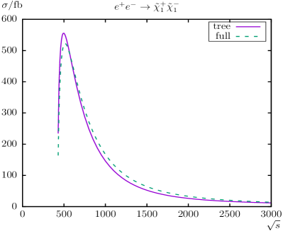
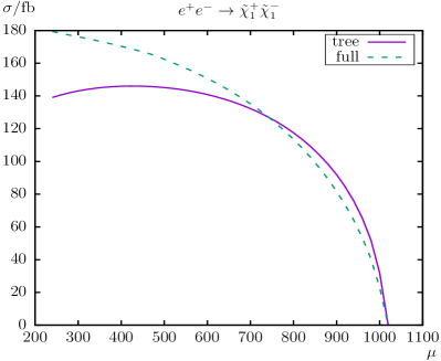
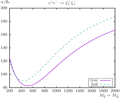
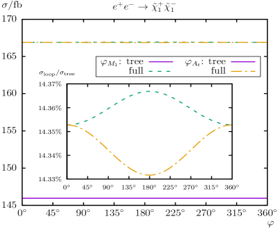
Figure 4: $\sigma(e^{+}e^{-}\to\tilde{\chi}_{1}^{+}\tilde{\chi}_{1}^{-})$. Tree-level and full one-loop corrected cross sections are shown with parameters chosen according to S1; see Tab. 1. The upper plots show the cross sections with $\sqrt{s}$ (left) and $\mu$ (right) varied; the lower plots show $M_{\tilde{L}}=M_{\tilde{E}}$ (left) and $\varphi_{M_{1}}$, $\varphi_{A_{t}}$ (right) varied.

In the analysis of the production cross section as a function of $\sqrt{s}$ (upper left plot) we find the expected behavior: a strong rise close to the production threshold, followed by a decrease with increasing $\sqrt{s}$. We find a very small shift w.r.t. $\sqrt{s}$ around the production threshold (not visible in the plot). Away from the production threshold, loop corrections of $\sim-8\,\%$ at $\sqrt{s}=500\,\,\mathrm{GeV}$ and $\sim+14\,\%$ at $\sqrt{s}=1000\,\,\mathrm{GeV}$ are found in scenario S1 (see Tab. 1), with a “tree crossing” (i.e. where the loop corrections become approximately zero and therefore cross the tree-level result) at $\sqrt{s}\approx 575\,\,\mathrm{GeV}$. The relative size of loop corrections increase with increasing $\sqrt{s}$ (and decreasing $\sigma$) and reach $\sim+19\,\%$ at $\sqrt{s}=3000\,\,\mathrm{GeV}$.

With increasing $\mu$ in S1 (upper right plot) we find a strong decrease of the production cross section, as can be expected from kinematics. The relative loop corrections in S1 reach $\sim+30\,\%$ at $\mu=240\,\,\mathrm{GeV}$ (at the border of the experimental limit), $\sim+14\,\%$ at $\mu=450\,\,\mathrm{GeV}$ (i.e. S1) and $\sim-30\,\%$ at $\mu=1000\,\,\mathrm{GeV}$. In the latter case these large loop corrections are due to the (relative) smallness of the tree-level results, which goes to zero for $\mu=1020\,\,\mathrm{GeV}$ (i.e. the chargino production threshold).

The cross section as a function of $M_{\tilde{L}}$ ($=M_{\tilde{E}}$) is shown in the lower left plot of Fig. 4. This mass parameter controls the $t$-channel exchange of first generation sleptons at tree-level. First a small decrease down to $\sim 90$ fb can be observed for $M_{\tilde{L}}\approx 400\,\,\mathrm{GeV}$. For larger $M_{\tilde{L}}$ the cross section rises up to $\sim 190$ fb for $M_{\tilde{L}}=2\,\,\mathrm{TeV}$. In scenario S1 we find a substantial increase of the cross sections from the loop corrections. They reach the maximum of $\sim+18\,\%$ at $M_{\tilde{L}}\approx 850\,\,\mathrm{GeV}$ with a nearly constant offset of about $20$ fb for higher values of $M_{\tilde{L}}$.

Due to the absence of $\varphi_{M_{1}}$ in the tree-level production cross section the effect of this complex phase is expected to be small. Correspondingly we find that the phase dependence $\varphi_{M_{1}}$ of the cross section in our scenario is tiny. The loop corrections are found to be nearly independent of $\varphi_{M_{1}}$ at the level below $\sim+0.1\,\%$ in S1. We also show the variation with $\varphi_{A_{t}}$, which enter via final state vertex corrections. While the variation with $\varphi_{A_{t}}$ is somewhat larger than with $\varphi_{M_{1}}$, it remains tiny and unobservable.

The analyses for the production cross sections of $\sigma(e^{+}e^{-}\to\tilde{\chi}_{1}^{\pm}\tilde{\chi}_{2}^{\mp})$ and $\sigma(e^{+}e^{-}\to\tilde{\chi}_{2}^{+}\tilde{\chi}_{2}^{-})$ can be found in Ref. [21]. To summarize, for the chargino pair production a decreasing cross section $\propto 1/s$ for $s\to\infty$ was observed, see Ref. [36]. The full one-loop corrections are very roughly 10-20 % of the tree-level results, but depend strongly on the size of $\mu$, where larger values result even in negative loop corrections. The cross sections are largest for $e^{+}e^{-}\to\tilde{\chi}_{1}^{+}\tilde{\chi}_{1}^{-}$ and $e^{+}e^{-}\to\tilde{\chi}_{2}^{+}\tilde{\chi}_{2}^{-}$ and roughly smaller by one order of magnitude for $e^{+}e^{-}\to\tilde{\chi}_{1}^{\pm}\tilde{\chi}_{2}^{\mp}$. This is because there is no $\gamma\,\tilde{\chi}_{1}^{\pm}\tilde{\chi}_{2}^{\mp}$ coupling at tree level in the MSSM.

We now turn to the neutralino production cross sections. First, the process $e^{+}e^{-}\to\tilde{\chi}_{1}^{0}\tilde{\chi}_{1}^{0}$ is shown in Fig. 5. Away from the production threshold, loop corrections of $\sim+13\,\%$ at $\sqrt{s}=1000\,\,\mathrm{GeV}$ are found in scenario S1 (see Tab. 1), with a maximum of nearly 7 fb at $\sqrt{s}\approx 2000\,\,\mathrm{GeV}$. The relative size of the loop corrections increase with increasing $\sqrt{s}$ and reach $\sim+22\,\%$ at $\sqrt{s}=3000\,\,\mathrm{GeV}$.

With increasing $\mu$ in S1 (upper right plot) we find a strong decrease of the production cross section, as can be expected from kinematics, discussed above. The relative loop corrections reach $\sim+14\,\%$ at $\mu=240\,\,\mathrm{GeV}$ (at the border of the experimental exclusion bounds) and $\sim+13\,\%$ at $\mu=450\,\,\mathrm{GeV}$ (i.e. S1). The tree crossing takes place at $\mu\approx 1600\,\,\mathrm{GeV}$. For higher $\mu$ values the loop corrections are negative, where the relative size becomes large due to the (relative) smallness of the tree-level results, which goes to zero for $\mu\approx 2000\,\,\mathrm{GeV}$.

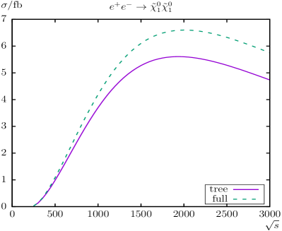
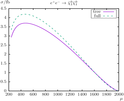
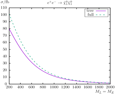
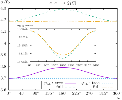
Figure 5: $\sigma(e^{+}e^{-}\to\tilde{\chi}_{1}^{0}\tilde{\chi}_{1}^{0})$. Tree-level and full one-loop corrected cross sections are shown with parameters chosen according to S1; see Tab. 1. The upper plots show the cross sections with $\sqrt{s}$ (left) and $\mu$ (right) varied; the lower plots show $M_{\tilde{L}}=M_{\tilde{E}}$ (left) and $\varphi_{M_{1}}$, $\varphi_{A_{t}}$ (right) varied.

The cross sections are decreasing with increasing $M_{\tilde{L}}$, i.e. the (negative) interference of the $t$-channel exchange decreases the cross sections, and the full one-loop result has its maximum of $\sim 100$ fb at $M_{\tilde{L}}=200\,\,\mathrm{GeV}$. Analogously the relative corrections are decreasing from $\sim+27\,\%$ at $M_{\tilde{L}}=200\,\,\mathrm{GeV}$ to $\sim+12\,\%$ at $M_{\tilde{L}}=2000\,\,\mathrm{GeV}$. For the other parameter variations one can conclude that a cross section larger by nearly one order of magnitude can be possible for very low $M_{\tilde{L}}$ (which are not yet excluded experimentally).

Now we turn to the complex phase dependence. As for the chargino production, $\varphi_{A_{t}}$ enters only via final state vertex corrections. On the other hand, $\varphi_{M_{1}}$ enters already at tree-level, and correspondingly larger effects are expected. We find that the phase dependence $\varphi_{M_{1}}$ of the cross section in S1 is small (lower right plot), possibly not completely negligible, amounting up to $\sim 2.3\,\%$ for the full corrections. The loop corrections at the level of $\sim+13\,\%$ are found to be nearly independent of $\varphi_{M_{1}}$, with a relative variation of $\sigma_{\text{loop}}/\sigma_{\text{tree}}$ at the level of $\sim+0.2\,\%$, (see the inlay in the lower right plot of Fig. 5). The loop effects of $\varphi_{A_{t}}$ are found at the same level as the ones of $\varphi_{M_{1}}$, i.e. rather negligible.

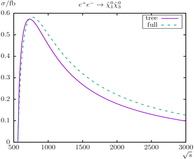
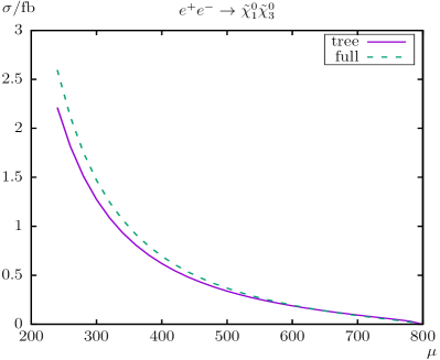
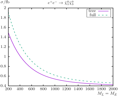
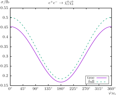
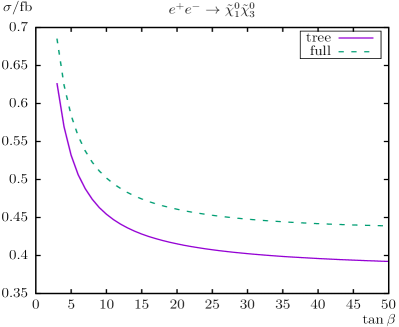
Figure 6: $\sigma(e^{+}e^{-}\to\tilde{\chi}_{1}^{0}\tilde{\chi}_{3}^{0})$. Tree-level and full one-loop corrected cross sections are shown with parameters chosen according to S1; see Tab. 1. The upper plots show the cross sections with $\sqrt{s}$ (left) and $\mu$ (right) varied; the middle plots show $M_{\tilde{L}}=M_{\tilde{E}}$ (left) and $\varphi_{M_{1}}$ (right) varied; the lower plot shows the variation with $t_{\beta}$.

Second, the process $e^{+}e^{-}\to\tilde{\chi}_{1}^{0}\tilde{\chi}_{3}^{0}$ shown in Fig. 6, which is found to be rather small of ${\cal O}(1\,\mbox{fb})$. As a function of $\sqrt{s}$ (upper row, left plot) we find a small shift w.r.t. $\sqrt{s}$ directly at the production threshold, as well as a shift of $\sim+50\,\,\mathrm{GeV}$ of the maximum cross section position. The loop corrections range from $\sim+11\,\%$ at $\sqrt{s}=1000\,\,\mathrm{GeV}$ (i.e. S1) to $\sim+28\,\%$ at $\sqrt{s}=3000\,\,\mathrm{GeV}$.

The dependence on $\mu$ (upper right plot) is rather small. The relative corrections are $\sim+17\,\%$ at $\mu=240\,\,\mathrm{GeV}$, $\sim+11\,\%$ at $\mu=450\,\,\mathrm{GeV}$ (i.e. S1), and have a tree crossing at $\mu\approx 650\,\,\mathrm{GeV}$. For larger $\mu$ the cross section goes to zero due to kinematics.

The cross section decreases with $M_{\tilde{L}}$ (middle left plot), again due to the negative interference of the $t$-channel contribution. The full correction has a maximum of $\sim 2$ fb for $M_{\tilde{L}}=200\,\,\mathrm{GeV}$, going down to $\sim 0.5$ fb at $M_{\tilde{L}}=2000\,\,\mathrm{GeV}$. Analogously the relative corrections are decreasing from $\sim+28\,\%$ at $M_{\tilde{L}}=200\,\,\mathrm{GeV}$ to $\sim+8\,\%$ at $M_{\tilde{L}}=2000\,\,\mathrm{GeV}$.

The phase dependence $\varphi_{M_{1}}$ of the cross section in S1 is shown in the middle right plot of Fig. 6. It is very pronounced and can vary $\sigma_{\text{full}}(e^{+}e^{-}\to\tilde{\chi}_{1}^{0}\tilde{\chi}_{3}^{0})$ by 60 %. The (relative) loop corrections are at the level of $\sim 10\,\%$ w.r.t. the tree cross section.

Here we also show the variation with $t_{\beta}$ in the lower plot of Fig. 6. The loop corrected cross section decreases from $\sim 0.7$ fb at small $t_{\beta}$ to $\sim 0.45$ fb at $t_{\beta}=50$. The relative corrections for the $t_{\beta}$ dependence are increasing from $\sim+9\,\%$ at $t_{\beta}=3$ to $\sim+12\,\%$ at $t_{\beta}=50$.

The numerical analysis of the other neutralino production cross sections can be found in Ref. [21]. To summarize, for the neutralino pair production the leading order corrections can reach a level of ${\cal O}(10\,\mbox{fb})$, depending on the SUSY parameters, but is very small for the production of two equal higgsino dominated neutralinos at the ${\cal O}(10\,\mbox{ab})$ level. This renders these processes difficult to observe at an $e^{+}e^{-}$ collider. Having both beams polarized could turn out to be crucial to yield a detectable production cross section in this case; see Ref. [37] for related analyses.

The full one-loop corrections are very roughly 10-20 % of the tree-level results, but vary strongly on the size of $\mu$ and $M_{\tilde{L}}$. Depending on the size of in particular these two parameters the loop corrections can be either positive or negative. This shows that the loop corrections, while being large, have to be included point-by-point in any precision analysis. The dependence on $\varphi_{M_{1}}$ was found at the level of $\sim 15\,\%$, but can go up to $\sim 40\,\%$ for the extreme cases. The relative loop corrections varied by up to $5\,\%$ with $\varphi_{M_{1}}$. Consequently, the complex phase dependence must be taken into account as well.

3.2 The processes $e^{+}e^{-}\to\mathrm{\tilde{e}}^{\pm}_{gs}\mathrm{\tilde{e}}^{\mp}_{gs^{\prime}}$ and $e^{+}e^{-}\to\tilde{\nu}_{g}\tilde{\nu}_{g}$

The SUSY parameters for the numerical analysis here (i.e.  in Ref. [22]) are chosen according to the scenario S2, shown in Tab. 2. This scenario is viable for the various cMSSM slepton production modes, again not picking specific parameters for each cross section. They are in particular in agreement with the relevant SUSY searches of ATLAS and CMS: Our electroweak spectrum is not covered by the latest ATLAS/CMS exclusion bounds, where two limits have to be distinguished. The limits not taking into account a possible intermediate slepton exclude a lightest neutralino only well below $300\,\,\mathrm{GeV}$ [38, 39], whereas in S2 we have $m_{\tilde{\chi}_{1}^{0}}\approx 323\,\,\mathrm{GeV}$. Limits with intermediary sleptons often assume a chargino decay to lepton and sneutrino, while in our scenario $m_{\tilde{\chi}_{1}^{\pm}}<m_{\tilde{\nu}_{e,\mu,\tau}}$. Furthermore, the exclusion bounds given in the $m_{\tilde{\chi}_{1}^{0}}$-$m_{\tilde{\chi}_{2}^{0}}$ mass plane (with $m_{\tilde{\chi}_{2}^{0}}\approx m_{\tilde{\chi}_{1}^{\pm}}$ assumed) above $m_{\tilde{\chi}_{2}^{0}}\sim 300\,\,\mathrm{GeV}$ do not cover a compressed spectrum [38, 40] for $\tilde{\chi}_{1}^{0}$, $\tilde{\chi}_{2}^{0}$, and $\tilde{\chi}_{1}^{\pm}$. In particular our scenario S2 assumed masses of $m_{\tilde{\chi}_{1}^{0}}\approx 323\,\,\mathrm{GeV}$ and $m_{\tilde{\chi}_{2}^{0}}\approx 354\,\,\mathrm{GeV}$, which are not excluded.

Table 2: MSSM default parameters for the numerical investigation; all parameters (except of $t_{\beta}$) are in GeV. The values for the trilinear sfermion Higgs couplings, $A_{f}$ are chosen to be real (except for $A_{\mathrm{e}_{g}}$ which can be complex) and such that charge- and/or color-breaking minima are avoided [31]. It should be noted that we chose common values $M_{\tilde{Q},\tilde{U},\tilde{D}}=2000\,\,\mathrm{GeV}$ for all squark generations, and $M_{\tilde{L}}=M_{\tilde{E}}+50\,\,\mathrm{GeV}$ for all slepton generations.

Scen.	$\sqrt{s}$	$t_{\beta}$	$\mu$	$M_{H^{\pm}}$	$M_{\tilde{Q},\tilde{U},\tilde{D}}$	$M_{\tilde{E}}$	$A_{\mathrm{u}_{g}}$	$A_{\mathrm{d}_{g}}$	$|A_{\mathrm{e}_{g}}|$	$|M_{1}|$	$M_{2}$	$M_{3}$
S2	1000	10	350	1200	2000	300	2600	2000	2000	400	600	2000

As in the previous subsection higher-order corrected Higgs-boson masses do not enter our calculation. However, as before, we ensured that over larger parts of the parameter space the lightest Higgs-boson mass is around $\sim 125\pm 3\,\,\mathrm{GeV}$ to indicate the phenomenological validity of our scenarios.

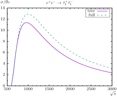
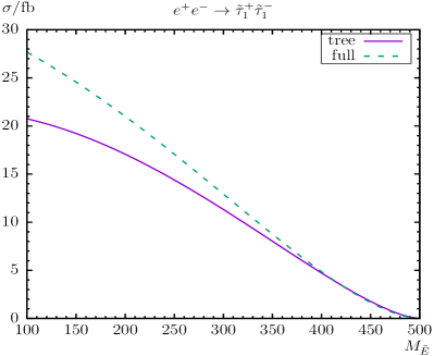
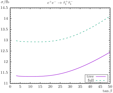
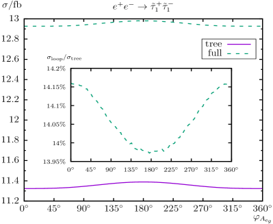
Figure 7: $\sigma(e^{+}e^{-}\to\tilde{\tau}^{+}_{1}\tilde{\tau}^{-}_{1})$. Tree-level and full one-loop corrected cross sections are shown with parameters chosen according to S2; see Tab. 2. The upper plots show the cross sections with $\sqrt{s}$ (left) and $M_{\tilde{E}}$ (right) varied; the lower plots show $t_{\beta}$ (left) and $\varphi_{A_{\mathrm{e}_{g}}}$ (right) varied. All masses and energies are in GeV.

As an example of the numerical analysis that will be presented in Ref. [22] we show the process $e^{+}e^{-}\to\tilde{\tau}^{+}_{1}\tilde{\tau}^{-}_{1}$ in Fig. 7. As a function of $\sqrt{s}$ we find loop corrections of $\sim+14\,\%$ at $\sqrt{s}=1000\,\,\mathrm{GeV}$ (i.e. S2), a tree crossing at $\sqrt{s}\approx 725\,\,\mathrm{GeV}$ (where the one-loop corrections are between $\pm 10\,\%$ for $\sqrt{s}\;\raisebox{-3.00003pt}{$\stackrel{{\scriptstyle\displaystyle<}}{{\sim}}$}\;900\,\,\mathrm{GeV}$) and $\sim+35\,\%$ at $\sqrt{s}=3000\,\,\mathrm{GeV}$.

In the analysis as a function of $M_{\tilde{E}}$ (upper right plot) the cross sections are decreasing with increasing $M_{\tilde{E}}$ as obvious from kinematics and the full corrections have their maximum of $\sim 28\,\mbox{fb}$ at $M_{\tilde{E}}=100\,\,\mathrm{GeV}$, more than two times larger than in S2. The relative corrections are changing from $\sim+33\,\%$ at $M_{\tilde{E}}=100\,\,\mathrm{GeV}$ to $\sim-25\,\%$ at $M_{\tilde{E}}=490\,\,\mathrm{GeV}$ with a tree crossing at $M_{\tilde{E}}=415\,\,\mathrm{GeV}$.

In the lower left row of Fig. 7 we show the dependence on $t_{\beta}$. The relative corrections for the $t_{\beta}$ dependence vary between $\sim+14.2\,\%$ at $t_{\beta}=5$ and $\sim+13.4\,\%$ at $t_{\beta}=50$.

The phase dependence $\varphi_{A_{\mathrm{e}_{g}}}$ of the cross section in S2 is shown in the lower right plot of Fig. 7. The loop correction increases the tree-level result by $\sim+14\,\%$. The phase dependence of the relative loop correction is very small and found to be below $0.2\,\%$. The variation with $\varphi_{M_{1}}$ is negligible and therefore not shown here.

The production cross sections for the other sleptons will be published in Ref. [22].

4 Conclusions

We have reviewed the calculation of chargino/neutralino/slepton production modes at $e^{+}e^{-}$ colliders with a two-particle final state, i.e. $e^{+}e^{-}\to\tilde{\chi}_{c}^{\pm}\tilde{\chi}_{c^{\prime}}^{\mp}$, $e^{+}e^{-}\to\tilde{\chi}_{n}^{0}\tilde{\chi}_{n^{\prime}}^{0}$, $e^{+}e^{-}\to\mathrm{\tilde{e}}^{\pm}_{gs}\mathrm{\tilde{e}}^{\mp}_{gs^{\prime}}$ and $e^{+}e^{-}\to\tilde{\nu}_{g}\tilde{\nu}_{g}$ allowing for complex parameters, as given in Refs. [21, 22]. In the case of a discovery of charginos, neutralinos or sleptons a subsequent precision measurement of their properties will be crucial to determine their nature and the underlying (SUSY) parameters. In order to yield a sufficient accuracy, one-loop corrections to the various chargino/neutralino/slepton production modes have to be considered. This is particularly the case for the high anticipated accuracy of the chargino/neutralino/slepton property determination at $e^{+}e^{-}$ colliders [12].

The evaluation of the processes (1) – (4) in Refs. [21, 22] is based on a full one-loop calculation, also including hard and soft QED radiation. The renormalization is chosen to be identical as for the various chargino/neutralino/slepton decay calculations; see, e.g. Refs. [15, 16, 17, 18] or chargino/neutralino/slepton production from heavy Higgs boson decay; see, e.g. Refs. [19, 20]. Consequently, the predictions for the production and decay can be used together in a consistent manner (e.g. in a global phenomenological analysis of the chargino/neutralino sector at the one-loop level).

For the analysis standard parameter sets (see Tabs. 1, 2) were chosen, that allow the production of all combinations of charginos/neutralinos or sleptons at an $e^{+}e^{-}$ collider with a center-of-mass energy up to $\sqrt{s}=1000\,\,\mathrm{GeV}$.

The review of the numerical analyses in Refs. [21, 22] showed the following. For the chargino pair production, $e^{+}e^{-}\to\tilde{\chi}_{c}^{\pm}\tilde{\chi}_{c^{\prime}}^{\mp}$, we observed an decreasing cross section $\propto 1/s$ for $s\to\infty$. The full one-loop corrections are very roughly 10-20 % of the tree-level results, but depend strongly on the size of $\mu$, where larger values result even in negative loop corrections. The cross sections are largest for $e^{+}e^{-}\to\tilde{\chi}_{1}^{+}\tilde{\chi}_{1}^{-}$ and $e^{+}e^{-}\to\tilde{\chi}_{2}^{+}\tilde{\chi}_{2}^{-}$ and roughly smaller by one order of magnitude for $e^{+}e^{-}\to\tilde{\chi}_{1}^{\pm}\tilde{\chi}_{2}^{\mp}$ due to the absence of the $\gamma\,\tilde{\chi}_{1}^{\pm}\tilde{\chi}_{2}^{\mp}$ coupling at tree level in the MSSM. The variation of the cross sections with $\varphi_{M_{1}}$ or $\varphi_{A_{t}}$ is found extremely small and the dependence on other phases were found to be roughly at the same level and have not been shown explicitely.

For the neutralino pair production, $e^{+}e^{-}\to\tilde{\chi}_{n}^{0}\tilde{\chi}_{n^{\prime}}^{0}$, the cross section can reach a level of ${\cal O}(10\,\mbox{fb})$, depending on the SUSY parameters, but is very small for the production of two equal higgsino dominated neutralinos at the ${\cal O}(10\,\mbox{ab})$. This renders these processes difficult to observe at an $e^{+}e^{-}$ collider. Having both beams polarized could turn out to be crucial to yield a detectable production cross section in this case. The full one-loop corrections are very roughly 10-20 % of the tree-level results, but vary strongly on the size of $\mu$ and $M_{\tilde{L}}$. Depending on the size of in particular these two parameters the loop corrections can be either positive or negative. The dependence on $\varphi_{M_{1}}$ was found to reach up to $\sim 15\,\%$, but can go up to $\sim 40\,\%$ for the extreme cases. The (relative) loop corrections varied by up to $5\,\%$ with $\varphi_{M_{1}}$.

In the example shown for slepton production, $\sigma(e^{+}e^{-}\to\tilde{\tau}^{+}_{1}\tilde{\tau}^{-}_{1})$, the loop corrections are found at the level of about $\sim\pm 15\%$, but vary strongly on the size of $M_{\tilde{E}}$. While the phase and $t_{\beta}$ dependence is rather small, it can be larger for the other slepton production processes; see Ref. [22].

The given examples show that the loop corrections, including the complex phase dependence, have to be included point-by-point in any precision analysis, or any precise determination of (SUSY) parameters from the production of cMSSM charginos/neutralinos/sleptons at $e^{+}e^{-}$ linear colliders.

We emphasize again that our full one-loop calculation can readily be used together with corresponding full one-loop corrections to chargino/neutralino/slepton decays [15, 16, 17, 18] or other chargino/neutralino/slepton production modes [19, 20].

Acknowledgements

The work of S.H. is supported in part by the MEINCOP Spain under contract FPA2016-78022-P, in part by the “Spanish Agencia Estatal de Investigación” (AEI) and the EU “Fondo Europeo de Desarrollo Regional” (FEDER) through the project FPA2016-78022-P, and in part by the AEI through the grant IFT Centro de Excelencia Severo Ochoa SEV-2016-0597.

References

- [1]
-
[2]
H. Nilles,
Phys. Rept. 110 (1984) 1;
R. Barbieri, Riv. Nuovo Cim. 11 (1988) 1. - [3] H. Haber, G. Kane, Phys. Rept. 117 (1985) 75.
- [4] J. Gunion, H. Haber, Nucl. Phys. B 272 (1986) 1.
- [5] S. Heinemeyer, Int. J. Mod. Phys. A 21 (2006) 2659 [arXiv:hep-ph/0407244].
- [6] A. Djouadi, Phys. Rept. 459 (2008) 1 [arXiv:hep-ph/0503173].
- [7] S. Heinemeyer, W. Hollik and G. Weiglein, Phys. Rept. 425 (2006) 265 [arXiv:hep-ph/0412214].
- [8] S. Heinemeyer, IFT–UAM/CSIC–18-003.
- [9] H. Baer et al., The International Linear Collider Technical Design Report - Volume 2: Physics, arXiv:1306.6352 [hep-ph].
-
[10]
R.-D. Heuer et al. [TESLA Collaboration], TESLA Technical
Design Report, Part III: Physics at an Linear Collider,
arXiv:hep-ph/0106315, see:
http://tesla.desy.de/new_pages/TDR_CD/start.html ;
K. Ackermann et al., DESY-PROC-2004-01. -
[11]
J. Brau et al. [ILC Collaboration],
ILC Reference Design Report Volume 1 - Executive Summary,
arXiv:0712.1950 [physics.acc-ph];
A. Djouadi et al. [ILC Collaboration], International Linear Collider Reference Design Report Volume 2: Physics at the ILC, arXiv:0709.1893 [hep-ph]. - [12] G. Moortgat-Pick et al., Eur. Phys. J. C 75 (2015) 8, 371 [arXiv:1504.01726 [hep-ph]].
-
[13]
L. Linssen, A. Miyamoto, M. Stanitzki and H. Weerts,
arXiv:1202.5940 [physics.ins-det];
H. Abramowicz et al. [CLIC Detector and Physics Study Collaboration], Physics at the CLIC Linear Collider – Input to the Snowmass process 2013, arXiv:1307.5288 [hep-ex]. -
[14]
G. Weiglein et al. [LHC/ILC Study Group],
Phys. Rept. 426 (2006) 47
[arXiv:hep-ph/0410364];
A. De Roeck et al., Eur. Phys. J. C 66 (2010) 525 [arXiv:0909.3240 [hep-ph]];
A. De Roeck, J. Ellis and S. Heinemeyer, CERN Cour. 49N10 (2009) 27. - [15] S. Heinemeyer and C. Schappacher, Eur. Phys. J. C 72 (2012) 2136 [arXiv:1204.4001 [hep-ph]].
-
[16]
S. Heinemeyer, F. von der Pahlen and C. Schappacher,
Eur. Phys. J. C 72 (2012) 1892
[arXiv:1112.0760 [hep-ph]];
S. Heinemeyer, F. von der Pahlen and C. Schappacher, arXiv:1202.0488 [hep-ph]. - [17] A. Bharucha, S. Heinemeyer, F. von der Pahlen and C. Schappacher, Phys. Rev. D 86 (2012) 075023 [arXiv:1208.4106 [hep-ph]].
- [18] A. Bharucha, S. Heinemeyer and F. von der Pahlen, Eur. Phys. J. C 73 (2013) 2629 [arXiv:1307.4237 [hep-ph]].
- [19] S. Heinemeyer and C. Schappacher, Eur. Phys. J. C 75 (2015) 5, 198 [arXiv:1410.2787 [hep-ph]].
- [20] S. Heinemeyer and C. Schappacher, Eur. Phys. J. C 75 (2015) 5, 230 [arXiv:1503.02996 [hep-ph]].
- [21] S. Heinemeyer and C. Schappacher, Eur. Phys. J. C 77 (2017) 9, 649 [arXiv:1704.07627 [hep-ph]].
- [22] S. Heinemeyer and C. Schappacher, in preparation, IFT–UAM/CSIC–18-007.
-
[23]
J. Küblbeck, M. Böhm and A. Denner,
Comput. Phys. Commun. 60 (1990) 165;
T. Hahn, Comput. Phys. Commun. 140 (2001) 418 [arXiv:hep-ph/0012260];
T. Hahn and C. Schappacher, Comput. Phys. Commun. 143 (2002) 54 [arXiv:hep-ph/0105349]. Program, user’s guide and model files are available via:
http://www.feynarts.de . - [24] T. Fritzsche, T. Hahn, S. Heinemeyer, F. von der Pahlen, H. Rzehak and C. Schappacher, Comput. Phys. Commun. 185 (2014) 1529 [arXiv:1309.1692 [hep-ph]].
-
[25]
T. Hahn and M. Pérez-Victoria,
Comput. Phys. Commun. 118 (1999) 153
[arXiv:hep-ph/9807565].
Program and user’s guide are available via:
http://www.feynarts.de/formcalc/ ;
http://www.feynarts.de/looptools/ . -
[26]
S. Heinemeyer, H. Rzehak and C. Schappacher,
Phys. Rev. D 82 (2010) 075010
[arXiv:1007.0689 [hep-ph]];
S. Heinemeyer, H. Rzehak and C. Schappacher, PoSCHARGED 2010 (2010) 039 [arXiv:1012.4572 [hep-ph]]. - [27] T. Fritzsche, S. Heinemeyer, H. Rzehak and C. Schappacher, Phys. Rev. D 86 (2012) 035014 [arXiv:1111.7289 [hep-ph]].
- [28] S. Heinemeyer and C. Schappacher, Eur. Phys. J. C 72 (2012) 1905 [arXiv:1112.2830 [hep-ph]].
- [29] S. Heinemeyer and C. Schappacher, Eur. Phys. J. C 76 (2016) 4, 220 [arXiv:1511.06002 [hep-ph]].
- [30] S. Heinemeyer and C. Schappacher, Eur. Phys. J. C 76 (2016) 10, 535 [arXiv:1606.06981 [hep-ph]].
-
[31]
J. Frère, D. Jones and S. Raby,
Nucl. Phys. B 222 (1983) 11;
M. Claudson, L. Hall and I. Hinchliffe, Nucl. Phys. B 228 (1983) 501;
C. Kounnas, A. Lahanas, D. Nanopoulos and M. Quiros, Nucl. Phys. B 236 (1984) 438;
J. Gunion, H. Haber and M. Sher, Nucl. Phys. B 306 (1988) 1;
J. Casas, A. Lleyda and C. Muñoz, Nucl. Phys. B 471 (1996) 3 [arXiv:hep-ph/9507294];
P. Langacker and N. Polonsky, Phys. Rev. D 50 (1994) 2199 [arXiv:hep-ph/9403306];
A. Strumia, Nucl. Phys. B 482 (1996) 24 [arXiv:hep-ph/9604417]. - [32] C. Patrignani et al. (Particle Data Group), Chin. Phys. C 420 (2016) 100001.
-
[33]
S. Amoroso,
talk given at “Moriond QCD”, March 2017, see:
https://moriond.in2p3.fr/QCD/2017/TuesdayMorning/Amoroso.pdf ;
https://twiki.cern.ch/twiki/bin/view/AtlasPublic/SupersymmetryPublicResults . -
[34]
M. Marionneau,
talk given at “Moriond EWK”, March 2017, see:
https://indico.in2p3.fr/event/13763/session/4/contribution/44/material/slides/1.pdf ;
R. Patel, talk given at “Moriond QCD”, March 2017, see:
https://moriond.in2p3.fr/QCD/2017/TuesdayMorning/Patel.pdf ;
https://twiki.cern.ch/twiki/bin/view/CMSPublic/PhysicsResultsSUS . -
[35]
S. Heinemeyer, W. Hollik and G. Weiglein,
Comput. Phys. Commun. 124 (2000) 76
[arXiv:hep-ph/9812320];
S. Heinemeyer, W. Hollik and G. Weiglein, Eur. Phys. J. C 9 (1999) 343 [arXiv:hep-ph/9812472];
G. Degrassi, S. Heinemeyer, W. Hollik, P. Slavich and G. Weiglein, Eur. Phys. J. C 28 (2003) 133 [arXiv:hep-ph/0212020];
M. Frank et al., JHEP 0702 (2007) 047 [arXiv:hep-ph/0611326];
T. Hahn, S. Heinemeyer, W. Hollik, H. Rzehak and G. Weiglein, Comput. Phys. Commun. 180 (2009) 1426;
T. Hahn, S. Heinemeyer, W. Hollik, H. Rzehak and G. Weiglein, Phys. Rev. Lett. 112 (2014) 14, 141801 [arXiv:1312.4937 [hep-ph]];
H. Bahl and W. Hollik, Eur. Phys. J. C 76 (2016) 499 [arXiv:1608.01880 [hep-ph]];
H. Bahl, S. Heinemeyer, W. Hollik and G. Weiglein, arXiv:1706.00346 [hep-ph], see:
http://www.feynhiggs.de . - [36] A. Bartl, H. Fraas and W. Majerotto, Z. Phys. C 30 (1986) 441.
- [37] G. Moortgat-Pick et al., Phys. Rept. 460 (2008) 131 [arXiv:hep-ph/0507011].
-
[38]
ATLAS Collaboration, ATLAS-CONF-2017-039, see:
https://atlas.web.cern.ch/Atlas/GROUPS/PHYSICS/CONFNOTES/ATLAS-CONF-2017-039 . -
[39]
CMS Collaboration, CMS-PAS-SUS-17-004, see:
http://cms-results.web.cern.ch/cms-results/public-results/preliminary-results/SUS-17-004/index.html . -
[40]
CMS Collaboration, CMS-PAS-SUS-16-039, see:
http://cms-results.web.cern.ch/cms-results/public-results/preliminary-results/SUS-16-039/index.html . - [41]