Stabilizing Unstable Periodic Orbits with Delayed Feedback Control
in Act-and-Wait Fashion

Abstract

A delayed feedback control framework for stabilizing unstable periodic orbits of linear periodic time-varying systems is proposed. In this framework, act-and-wait approach is utilized for switching a delayed feedback controller on and off alternately at every integer multiples of the period of the system. By analyzing the monodromy matrix of the closed-loop system, we obtain conditions under which the closed-loop system’s state converges towards a periodic solution under our proposed control law. We discuss the application of our results in stabilization of unstable periodic orbits of nonlinear systems and present numerical examples to illustrate the efficacy of our approach.

1 Introduction

Stabilization of unstable periodic orbits of nonlinear systems using delayed feedback control was first explored in [1]. In the delayed feedback control scheme, the difference between the current state and the delayed state is utilized as a control input to stabilize an unstable orbit. The delay time is set to correspond to the period of the orbit to be stabilized so that the control input vanishes when the stabilization is achieved.

Delayed feedback controllers have been used in many studies for stabilization of the periodic orbits of both continuous- and discrete-time nonlinear systems (see, e.g., [2, 3, 4], and the references therein). More recently, [5] investigated delayed feedback control of nonlinear systems that are subject to noise, [6] explored delayed feedback control of a delay differential equation, and [7] utilized delayed feedback control for stabilizing quasi periodic orbits. The work [8] studied the relation between the delayed feedback control approach and the harmonic oscillator-based control methods for stabilizing periodic orbits in chaotic systems [9]. Furthermore, [10] and [11] explored the situation where the period of the orbit and the delay time in the delayed feedback controller do not match due to imperfect information about the periodic orbit or inaccuracies in the implementation of the controller.

The physical structure of delayed feedback control scheme is simple. However, the analysis of the closed-loop system is difficult. This is due to the fact that to investigate the system under delayed feedback control, one has to deal with delay-differential equations, the state space of which is infinite dimensional. To deal with the difficulties in the analysis of delay differential equations, an approach is to use approximation techniques (see, for instance, [12] and [13]). Another approach was taken in [14]. There, stabilization of a linear time-invariant system with a time-delay controller was considered, and “act-and-wait” concept was introduced. This concept is characterized by alternately applying and cutting off the controller in finite intervals. It is shown in [14] that by utilizing the act-and-wait concept, one may be able to derive a finite-sized monodromy matrix for the closed-loop system, which can then be used for stability analysis. Act-and-wait concept has been extended to discrete-time systems in [15], and tested through experiments in [16]. Furthermore, act-and-wait approach has been used together with delayed feedback control in [17] for stabilizing unstable fixed points of nonlinear systems, and more recently in [18] for stabilizing unstable periodic orbits of nonautonomous nonlinear systems.

In this paper, we explore the stabilization of periodic solutions to linear periodic systems with an act-and-wait-fashioned delayed feedback control framework.  In this framework, a switching mechanism is utilized to turn the delayed feedback controller on and off alternately at every integer multiple of the period of a given linear periodic system. Act-and-wait scheme allows us to obtain the monodromy matrix associated with the closed-loop system under our proposed controller. We then use the obtained monodromy matrix for obtaining conditions under which the closed-loop system’s state converges to a periodic solution. Our main motivation for studying a delayed feedback control problem for periodic systems stems from our desire to analyze the stability of a periodic orbit of a nonlinear system under delayed feedback control. In this paper we apply our results for linear periodic systems in analyzing periodic linear variational equations obtained after linearizing nonlinear systems (under delayed feedback control) around periodic trajectories corresponding to periodic orbits. The uncontrolled nonlinear systems that we consider are autonomous and as a result their stability assessment under the act-and-wait-fashioned delayed feedback controller differs from the nonautonomous case discussed in [18]. We also note that our delayed feedback control approach and therefore our analysis techniques differ from those in earlier works on stabilization of linear periodic systems where researchers have employed Gramian-based controllers [19], periodic Lyapunov functions [20], and linear matrix inequalities [21].

The paper is organized as follows. In Section 2, we introduce our act-and-wait-fashioned delayed feedback control framework for stabilizing periodic solutions of linear periodic systems; we present a method for assessing the asymptotic stability of a periodic solution of the closed-loop system under our proposed framework. Furthermore, in Section 3 we discuss an application of our results in stabilizing unstable periodic orbits of nonlinear systems. We present illustrative numerical examples in Section 4. Finally, we conclude our paper in Section 5.

We note that a preliminary version of this work was presented in [22]. In this paper, we provide additional discussions and examples.

2 Delayed Feedback Stabilization of Periodic Orbits

In this section, we provide the mathematical model for a linear periodic time-varying system and introduce a new delayed feedback control framework based on act-and-wait approach. We then characterize a method for evaluating convergence of state trajectories of a closed-loop linear time-varying periodic system towards a periodic solution.

2.1 Linear Periodic Time-Varying System

Consider the linear periodic time-varying system

$$\dot{x}(t) =A(t)x(t)+B(t)u(t),\quad x(t_{0})=x_{0},\quad t\geq t_{0},$$ (1)

where $x(t)\in\mathbb{R}^{n}$ is the state vector, $u(t)\in\mathbb{R}^{m}$ is the control input, and $A(t)\in\mathbb{R}^{n\times n}$ and $B(t)\in\mathbb{R}^{n\times m}$ are periodic matrices with period $T>0$, that is, $A(t+T)=A(t)$ and $B(t+T)=B(t)$, $t\geq t_{0}$. For simplicity of exposition, we assume $t_{0}=0$ for the rest of the discussion because the case where $t_{0}\neq 0$ can be similarly handled. Furthermore, we assume that the uncontrolled ($u(t)\equiv 0$) dynamics possess a periodic solution $x(t)\equiv x^{*}(t)$ with period $T$ satisfying $x^{*}(t+T)=x^{*}(t),\,t\geq 0$. It follows from Floquet’s theorem that there exists such a periodic solution to the uncontrolled system (1) of period $T$ if and only if there exists a nonsingular matrix $C\in\mathbb{R}^{n\times n}$ possessing $1$ in its spectrum such that $V(t+T)=V(t)C$, where $V(t)$ denotes a fundamental matrix of the uncontrolled system (1). Moreover, note that since $x(t)\equiv x^{*}(t)$ is a $T$-periodic solution of the uncontrolled system (1), $x(t)\equiv\alpha x^{*}(t)$ is also a $T$-periodic solution for all $\alpha\in\mathbb{R}$, that is, $x(t)\equiv\alpha x^{*}(t)$ satisfies (1) with $u(t)\equiv 0$.

We investigate the asymptotic stability of periodic solutions of the closed-loop system (1) under the delayed feedback control input

$$u(t) =-g(t)F(x(t)-x(t-T)),$$ (2)

where $F\in\mathbb{R}^{m\times n}$ is a constant gain matrix and

$$g(t) \triangleq\left\{\begin{array}[]{rl}0,&2kT\leq t<(2k+1)T,\\ 1,&(2k+1)T\leq t<2(k+1)T,\end{array}\right.\,k\in\mathbb{N}_{0}.$$ (5)

is a time-varying function that switches the controller on and off alternately at every integer multiples of the period $T$.

Note that the feedback term characterized in (2) vanishes after the periodic solution is stabilized. Specifically, for $x(t)\equiv x^{*}(t)$, we have $u(t)=0$, $t\geq 0$, since $x(t)=x(t-T)$.

We remark that our control approach is a specific case of the act-and-wait approach introduced in [14]. In particular, in our control law (2), both the acting and the waiting durations have length $T$. Specifically, in every $2T$ period, the controller first waits for a duration of length $T$, and then acts for a duration of length $T$. Note that the controllers in [14] are more general in the sense that acting and waiting times need not be equal. In Section 4, we also consider different switching functions $g(t)$ that lead to different acting and waiting times.

The reason why $g(t)$ is set to be a time-varying function can be understood if we compare it to the case where $g(t)$ is constant. For instance, if $g(t)\equiv 1$ in (2), then (1) becomes

$$\dot{x}(t) =(A(t)-B(t)F)x(t)+B(t)Fx(t-T),$$ (6)

which is a delay-differential equation. Analysis of the solution of (6) is difficult, as the state space associated with (6) is infinite-dimensional.

On the other hand, for the linear periodic system

$$\dot{x}(t) =A(t)x(t),\quad A(t)=A(t+T),$$ (7)

where there are no delay terms, stability of an equilibrium solution can be assessed by analyzing the corresponding monodromy matrix. Let $\Phi(\cdot,\cdot)$ denote the state-transition matrix of (7). The monodromy matrix associated with the $T$-periodic system (7) is given by $\Phi(T,0)\in\mathbb{R}^{n\times n}$. The eigenvalues of the monodromy matrix, known as the Floquet multipliers, are essential in the analysis of the long-term behavior of the state-transition matrix of (7), because

$$\Phi(t+kT,0) =\Phi(t,0)\Phi^{k}(T,0),\quad k\in\mathbb{N}_{0}.$$ (8)

Moreover, the state of the periodic system (7) satisfies

$$x((k+1)T) =\Phi x(kT),\quad k\in\mathbb{N}_{0}.$$

Observe that if $g(t)\equiv 1$ in (2), we would not be able to find a homogeneous expression in the form of (7), let alone find a corresponding “monodromy matrix”, because of the existence of the delay term.

However, in our case, following the act-and-wait approach, we define $g(t)$ as in (5) as a switching function. Consequently, we are able to construct a monodromy matrix $\Lambda\in\mathbb{R}^{n\times n}$ for the closed-loop system (1), (2) with the doubled period $2T$ such that

$$x(2(k+1)T) =\Lambda x(2kT),\quad k\in\mathbb{N}_{0}.$$ (9)

Note that the spectrum of the monodromy matrix $\Lambda$ characterizes long-term behavior of the state trajectory.

In the following sections, we first derive the monodromy matrix, and then we present conditions for the convergence of the state trajectory towards a periodic solution of the closed-loop system (1), (2).

2.2 Monodromy Matrix

In this section, we obtain the monodromy matrix associated with the closed-loop system given by (1), (2). In our derivations, we use $\Phi(\cdot,\cdot)$ to denote the state-transition matrix associated with (7). Furthermore, let $\Upsilon(\cdot,\cdot)$ denote the state-transition matrix for the linear $T$-periodic system

$$\dot{x}(t) =(A(t)-B(t)F)x(t).$$ (10)

Now, let $\mathcal{T}_{0}(k)\triangleq[2kT,(2k+1)T)$, $\mathcal{T}_{1}(k)\triangleq[(2k+1)T,2(k+1)T)$, $k\in\mathbb{N}_{0}$. Note that when $t\in\mathcal{T}_{1}(k)$, the controller is on, that is, $g(t)=1$. Hence, it follows from (1) and (2) that for $t\in\mathcal{T}_{1}(k)$,

$$\dot{x}(t) =(A(t)-B(t)F)x(t)+B(t)Fx(t-T).$$ (11)

Observe that for $t\in\mathcal{T}_{1}(k)$, we have $t-T\in\mathcal{T}_{0}(k)$. Since the controller is turned off during the interval $\mathcal{T}_{0}(k)$, the evolution of the state in this interval is described by (7) corresponding to the uncontrolled dynamics. Therefore, $x(t-T)$ can be expressed by

$$x(t-T) =\Phi(t-T,2kT)x(2kT),\quad t\in\mathcal{T}_{1}(k).$$ (12)

Now, by using (11) and (12), we obtain

$$\dot{x}(t) =(A(t)-B(t)F)x(t)$$

$$\quad+B(t)F\Phi(t-T,2kT)x(2kT),\quad t\in\mathcal{T}_{1}(k).$$ (13)

By multiplying both sides of (13) from left with the matrix $\Upsilon^{-1}(t,(2k+1)T)$, we obtain

$$\Upsilon^{-1}(t,(2k+1)T)\dot{x}(t)$$

$$\,\,=\Upsilon^{-1}(t,(2k+1)T)(A(t)-B(t)F)x(t)$$

$$\,\,\quad+\Upsilon^{-1}(t,(2k+1)T)B(t)F\Phi(t-T,2kT)x(2kT).$$ (14)

Since $\Upsilon^{-1}(t,(2k+1)T)(A(t)-B(t)F)=-\frac{\mathrm{d}}{\mathrm{d}t}\Upsilon^{-1}(t,(2k+1)T)$, we have

$$\Upsilon^{-1}(t,(2k+1)T)\dot{x}(t)$$

$$\quad-\Upsilon^{-1}(t,(2k+1)T)(A(t)-B(t)F)x(t)$$

$$=\Upsilon^{-1}(t,(2k+1)T)\dot{x}(t)+\frac{\mathrm{d}}{\mathrm{d}t}\Upsilon^{-1}(t,(2k+1)T)x(t)$$

$$=\frac{\mathrm{d}}{\mathrm{d}t}\big{(}\Upsilon^{-1}(t,(2k+1)T)x(t)\big{)}.$$ (15)

It follows from (14) and (15) that

$$\frac{\mathrm{d}}{\mathrm{d}t}\big{(}\Upsilon^{-1}(t,(2k+1)T)x(t)\big{)}$$

$$\quad=\Upsilon^{-1}(t,(2k+1)T)B(t)F\Phi(t-T,2kT)x(2kT).$$ (16)

Next, we integrate both sides of (16) over the interval $[(2k+1)T,t)$ to obtain

$$\Upsilon^{-1}(t,(2k+1)T)x(t)$$

$$\,\,=\Upsilon^{-1}((2k+1)T,(2k+1)T)x((2k+1)T)$$

$$\,\,\quad+\Big{(}\int_{(2k+1)T}^{t}\Upsilon^{-1}(s,(2k+1)T)B(s)F\Phi(s-T,2kT)\mathrm{d}s\Big{)}$$

$$\,\,\quad\cdot x(2kT).$$ (17)

Noting that $\Upsilon^{-1}((2k+1)T,(2k+1)T)=I_{n}$ and $x((2k+1)T)=\Phi((2k+1)T,2kT)x(2kT)$, we obtain

$$x(t)=\Upsilon(t,(2k+1)T)\Phi((2k+1)T,2kT)x(2kT)$$

$$\quad+\Upsilon(t,(2k+1)T)$$

$$\quad\cdot\Big{(}\int_{(2k+1)T}^{t}\Upsilon^{-1}(s,(2k+1)T)B(s)F\Phi(s-T,2kT)\mathrm{d}s\Big{)}$$

$$\quad\cdot x(2kT).$$ (18)

Since both (7) and (10) are $T$-periodic, we have $\Upsilon(t,(2k+1)T)=\Upsilon(t-(2k+1)T,0)$ and $\Phi((2k+1)T,2kT)=\Phi(T,0)$. Furthermore, since $\Upsilon(t,(2k+1)T)=\Upsilon(t,s)\Upsilon(s,(2k+1)T)$, $s\in[(2k+1)T,t]$, we have $\Upsilon(t,(2k+1)T)\Upsilon^{-1}(s,(2k+1)T)=\Upsilon(t,s)$. Consequently, it follows from (18) that

$$x(t)=\Big{(}\Upsilon(t-(2k+1)T,0)\Phi(T,0)$$

$$\,\,+\int_{(2k+1)T}^{t}\Upsilon(t,s)B(s)F\Phi(s-T,2kT)\mathrm{d}s\Big{)}x(2kT),$$ (19)

for $t\in\mathcal{T}_{1}(k)$. We now change the variable of the integral term in (19) by setting $\bar{s}=s-2kT$. As a result, we obtain

$$\int_{(2k+1)T}^{t}\Upsilon(t,s)B(s)F\Phi(s-T,2kT)\mathrm{d}s$$

$$\quad=\int_{T}^{t-2kT}\Upsilon(t,\bar{s}+2kT)B(\bar{s}+2kT)$$

$$\quad\quad\cdot F\Phi(\bar{s}+2kT-T,2kT)\mathrm{d}\bar{s},\quad t\in\mathcal{T}_{1}(k).$$ (20)

By $T$-periodicity of (7) and (10), we have $\Upsilon(t,\bar{s}+2kT)=\Upsilon(t-2kT,\bar{s})$ and $\Phi(\bar{s}+2kT-T,2kT)=\Phi(\bar{s}-T,0)$. Moreover, $B(\bar{s}+2kT)=B(\bar{s})$, since $B(\cdot)$ is a $T$-periodic matrix function. It then follows from (20) that

$$\int_{(2k+1)T}^{t}\Upsilon(t,s)B(s)F\Phi(s-T,2kT)\mathrm{d}s$$

$$\quad=\int_{T}^{t-2kT}\Upsilon(t-2kT,\bar{s})B(\bar{s})F\Phi(\bar{s}-T,0)\mathrm{d}\bar{s}.$$ (21)

Now, from (19) and (21), we obtain

$$x(t) =\Big{(}\Upsilon(t-(2k+1)T,0)\Phi(T,0)$$

$$\quad+\int_{T}^{t-2kT}\Upsilon(t-2kT,\bar{s})B(\bar{s})F\Phi(\bar{s}-T,0)\mathrm{d}\bar{s}\Big{)}$$

$$\quad\cdot x(2kT),\quad t\in\mathcal{T}_{1}(k).$$ (22)

By continuity of the state, we can compute $x(2(k+1)T)$ by using (22). Specifically, we set $t=2(k+1)T$ in (22) and obtain (9), where the monodromy matrix $\Lambda$ is given by

$$\Lambda =\Big{(}\Upsilon(T,0)\Phi(T,0)$$

$$\quad+\int_{T}^{2T}\Upsilon(2T,\bar{s})B(\bar{s})F\Phi(\bar{s}-T,0)\mathrm{d}\bar{s}\Big{)}.$$ (23)

Notice that (9) characterizes the evolution of the state at times $t=2kT$, $k\in\mathbb{N}_{0}$. Consequently, stability of the equilibrium solutions of the closed-loop system (1), (2) can be deduced through the eigenvalues of the monodromy matrix.

Moreover, note that $x^{*}(t)$ satisfies $x^{*}(2T)=x^{*}(0)$. In addition, from (9) we have

$$x^{*}(2T) =\Lambda x^{*}(0).$$ (24)

It follows that $x^{*}(0)=\Lambda x^{*}(0)$, and hence, the monodromy matrix $\Lambda$ associated with the closed-loop system (1), (2) possesses $1$ as an eigenvalue with the eigenvector $x^{*}(0)$. Note that both the algebraic and the geometric multiplicity of the eigenvalue $1$ may be greater than $1$.

Let $\kappa\in\{1,2,\ldots,n\}$ denote the algebraic multiplicity of the eigenvalue $1$. We represent generalized eigenvectors of the monodromy matrix $\Lambda$ by vectors $v_{1},v_{2},\ldots,v_{n}\in\mathbb{C}^{n}$ out of which $v_{1},v_{2}\ldots,v_{\kappa}\in\mathbb{R}^{n}$ denote the generalized eigenvectors associated with the eigenvalue $1$. The generalized eigenvectors $v_{1},v_{2},\ldots,v_{n}$ are linearly independent [23], and hence form a basis for $\mathbb{C}^{n}$, that is, for any $y\in\mathbb{C}^{n}$, there exist $\alpha_{1}$, $\alpha_{2}$, $\ldots$, $\alpha_{n-1}$, $\alpha_{n}\in\mathbb{C}$ such that $y=\sum_{i=1}^{n}\alpha_{i}v_{i}$. Note that $\alpha_{i}v_{i}$ characterizes the component of $y$ along $v_{i}$ (the $i$th element of the basis). Note also that linear independence of vectors $v_{1},v_{2},\ldots,v_{n}$ guarantees that the constants $\alpha_{1},\alpha_{2},\ldots,\alpha_{n}$ are uniquely determined.

The long-term behavior of the state trajectory is determined by the spectrum of the monodromy matrix $\Lambda$. In Theorem 2.1 below, we present the condition for the convergence of the state trajectory towards a periodic solution.

Theorem 2.1

Consider the linear time-varying periodic system (1) with the periodic solution $x^{*}(t)$. Let the initial condition be given by $x(0)=x_{0}\triangleq\sum_{i=1}^{n}\alpha_{i}v_{i}$, where $v_{1},v_{2},\ldots,v_{n}\in\mathbb{C}^{n}$ are the generalized eigenvectors of the monodromy matrix $\Lambda\in\mathbb{R}^{n\times n}$, and $\alpha_{1},\alpha_{2},\ldots,\alpha_{n}\in\mathbb{C}$. Suppose that $1$ is a semisimple eigenvalue of $\Lambda$. Let $\kappa\in\{1,2,\ldots,n\}$ denote the algebraic multiplicity of the eigenvalue $1$ associated with the eigenspace spanned by the eigenvectors $v_{1},v_{2}\ldots,v_{\kappa}\in\mathbb{R}^{n}$. If all the eigenvalues, other than the eigenvalue $1$ of the monodromy matrix $\Lambda$ are strictly inside the unit circle of the complex plane, then $\lim_{k\to\infty}x(2kT)=\sum_{i=1}^{\kappa}\alpha_{i}v_{i}$.

Proof. First, we define $P\triangleq\left[v_{1},v_{2},\ldots,v_{n}\right]$. Note that since the columns of the matrix $P$ given by $v_{1}$, $v_{2}$, $\ldots$, $v_{n}$ are linearly independent, it follows that $P$ is nonsingular.

Furthermore, note that with the similarity transformation $J\triangleq P^{-1}\Lambda P$, we obtain the Jordan form of the monodromy matrix $\Lambda$ such that $J=\mathrm{diag}[J_{1},J_{2},\ldots,J_{r}]$, where $r\in\mathbb{N}$ denotes the number of Jordan blocks, which is also equal to the sum of the geometric multiplicities of the eigenvalues of the monodromy matrix $\Lambda$. The Jordan blocks $J_{i}\in\mathbb{C}^{n_{i}\times n_{i}}$, $i\in\{1,2,\ldots,r\}$, have the form $J_{i}=\lambda_{i}I_{n_{i}}+N_{i}$, where $\lambda_{i}\in\mathbb{C}$ is an eigenvalue of the monodromy matrix $\Lambda$ and $N_{i}\in\mathbb{R}^{n_{i}\times n_{i}}$ is a nilpotent matrix of degree $n_{i}$.

We use (9), the definition for the Jordan form $J$ of the monodromy matrix $\Lambda$, and $[\alpha_{1},\alpha_{2},\ldots,\alpha_{n}]^{\mathrm{T}}=P^{-1}x_{0}$ to obtain

$$x(2kT) =\Lambda^{k}x_{0}$$

$$=PJ^{k}P^{-1}x_{0}$$

$$=P\mathrm{diag}[J_{1}^{k},J_{2}^{k},\ldots,J_{r}^{k}][\alpha_{1},\alpha_{2},\ldots,\alpha_{n}]^{\mathrm{T}}.$$ (25)

Note that the eigenvalue $1$, which has algebraic multiplicity $\kappa\in\{1,2,\ldots,n\}$, is a semisimple eigenvalue associated with the eigenvectors $v_{1},v_{2}\ldots,v_{\kappa}\in\mathbb{R}^{n}$. As a result, $J_{i}=1$, $i\in\{1,2,\ldots,\kappa\}$, and hence $\lim_{k\to\infty}J_{i}^{k}=1$, $i\in\{1,2,\ldots,\kappa\}$. On the other hand, for each $i\in\{\kappa+1,\kappa+2,\ldots,r\}$ the eigenvalue $\lambda_{i}$ is strictly inside the unit circle; therefore, $\lim_{k\to\infty}J_{i}^{k}=0$, $i\in\{\kappa+1,\kappa+2,\ldots,r\}$. Thus, $\lim_{k\to\infty}J^{k}$ takes the form of a diagonal matrix with $1$ as the first $\kappa$ diagonal entries and $0$ elsewhere. It follows from (25) that

$$\lim_{k\to\infty}x(2kT) =P\mathrm{diag}[\overbrace{1,\ldots,1}^{\kappa\,\mathrm{terms}},\overbrace{0,\ldots,0}^{n-\kappa\,\mathrm{terms}}]$$

$$\quad\cdot[\alpha_{1},\alpha_{2},\ldots,\alpha_{n}]^{\mathrm{T}}$$

$$=P[\alpha_{1},\ldots,\alpha_{\kappa},0,\ldots,0]^{\mathrm{T}}$$

$$=\sum_{i=1}^{\kappa}\alpha_{i}v_{i},$$ (26)

which completes the proof. $\square$

Under the condition in Theorem 2.1 that all the eigenvalues, other than the semisimple eigenvalue $1$, of the monodromy matrix $\Lambda$ are strictly inside the unit circle, the state evaluated at integer multiples of the doubled period $2T$ converges to a point on a periodic solution of the uncontrolled ($u(t)\equiv 0$) system (1). Hence, the state trajectory converges towards a periodic solution. The location of the limiting periodic solution depends on the initial condition $x_{0}$. Specifically, the state evaluated at integer multiples of the doubled period $2T$ converges to the point given by $\sum_{i=1}^{\kappa}\alpha_{i}v_{i}$, where $\alpha_{i}v_{i}$ characterizes the component of the initial state $x_{0}$ along the eigenvector $v_{i}$ associated with the eigenvalue $1$ of the monodromy matrix $\Lambda$. Note that if the algebraic multiplicity of the eigenvalue $1$ is $\kappa=1$, then the limiting periodic solution is given by $\alpha_{1}x^{*}(t)$, where $\alpha_{1}x^{*}(0)$ is the component of $x_{0}$ along the eigenvector $v_{1}=x^{*}(0)$.

3 Stabilization of Unstable Periodic Orbits of Nonlinear Systems

We now employ the results obtained for linear periodic systems for stabilizing an unstable periodic orbit of a nonlinear system.

Consider the nonlinear system given by

$$\dot{x}(t)=f(x(t))+u(t),\quad x(0)=x_{0},\quad t\geq 0,$$ (27)

where $x(t)\in\mathbb{R}^{n}$ is the state vector, $u(t)\in\mathbb{R}^{n}$ is the control input, and $f:\mathbb{R}^{n}\to\mathbb{R}^{n}$ is a nonlinear function. Suppose that the uncontrolled ($u(t)\equiv 0$) system (27) possesses a periodic solution $x(t)\equiv x^{*}(t)$ with a known period $T>0$ such that

$$x^{*}(t+T) =x^{*}(t),$$ (28)

$$\dot{x}^{*}(t) =f(x^{*}(t)),\quad t\in[0,\infty).$$ (29)

The periodic orbit associated with the periodic solution $x^{*}(\cdot)$ is given by $\mathcal{O}\triangleq\{x^{*}(t)\colon t\in[0,T)\}$. The stability of the periodic orbit $\mathcal{O}\subset\mathbb{R}^{n}$ is characterized through the stability of a fixed point of a Poincaré map defined on an $(n-1)$-dimensional hypersurface that is transversal to the periodic orbit (see [24, 25]). In this paper, we consider the case where $\mathcal{O}$ is an unstable periodic orbit (UPO) and discuss its stabilization.

There are several methods known for stabilizing the UPO. One of them is the Pyragas-type delayed feedback control framework (see [1, 3, 4]). In this framework the control input is given by

$$u(t)=-F(x(t)-x(t-T)),$$ (30)

where $F\in\mathbb{R}^{n\times n}$ is the gain matrix of the controller. The control input is computed based on the difference between the current state and the delayed state. The delay time is set to correspond to the period $T$ of the desired UPO so that the control input vanishes after the UPO is stabilized. In the delayed feedback control method, the controller uses the delayed state instead of the UPO as a reference signal to which the current state is desired to be stabilized. Therefore this method does not require a preliminary calculation of the UPO if its period is given.

The analysis of the closed-loop system under delayed feedback controller is difficult, because the closed-loop dynamics is described by a delay-differential equation (27), (30), the state space of which is infinite-dimensional. This fact is our motivation for employing the act-and-wait-fashioned delayed feedback control law (2), since the closed-loop system system (2), (27) can be analyzed by utilizing the methods that we developed in Section 2.

Remark 3.1

Act-and-wait-fashioned delayed-feedback control laws were previously used in [17] and [18] for different problem settings. In [17], the stabilization of a fixed-point is considered. Furthermore, in [18], periodic orbit stabilization is considered for a nonautonomous system. Specifically, the uncontrolled system in [18] is affected by an external periodic force, which induces the periodic orbit. The controller in [18] is designed so that all Floquet multipliers of the linearized system are strictly inside the unit circle of the complex plane. In our case, the uncontrolled system is not driven by a periodic force and it is autonomous. The periodic orbit in our case is embedded in the dynamics. The stability assessment method in this paper differs from that in [18] due to the difference in the analysis of autonomous and nonautonomous systems (see Section 7.1.3 of [26]). In particular, as we discuss below, the linearized system in our case always possesses $1$ as a Floquet multiplier regardless of the choice of the feedback gain matrix, and moreover, the stability of the periodic orbit under the act-and-wait-fashioned controller can be analyzed by assessing the Floquet multipliers that are not $1$.

We analyze the stability of the periodic orbit $\mathcal{O}\subset\mathbb{R}^{n}$ under the act-and-wait-fashioned control input by assessing the monodromy matrix for the linear variational equation associated with the closed-loop dynamics (2), (27). Specifically, we linearize the closed-loop system (2), (27) around the periodic trajectory $x^{*}(t)$. First, we write the solution of (2), (27) as

$$x(t)=x^{*}(t)+\delta x(t),$$ (31)

where $\delta x(t)$ is the state deviation from the periodic solution $x^{*}(t)$ at time $t$. It then follows from (27) and (31) that

$$\dot{x}^{*}(t)+\dot{\delta x}(t)$$

$$\quad=f(x^{*}(t)+\delta x(t))$$

$$\quad\quad-g(t)F(x^{*}(t)+\delta x(t)-x^{*}(t-T)-\delta x(t-T))$$

$$\quad=f(x^{*}(t))+{\left.\frac{\partial f(x)}{\partial x}\right|}_{x=x^{*}(t)}\delta x(t)+H.O.T.$$

$$\quad\quad-g(t)F(\delta x(t)-\delta x(t-T)),$$ (32)

where $H.O.T.$ denotes the higher-order terms in $\delta x$.

By using (29) and neglecting the higher-order terms for infinitely small deviations in (32), we obtain the linear variational equation

$$\dot{\delta x}(t)=A(t)\delta x(t)-g(t)F(\delta x(t)-\delta x(t-T)),$$ (33)

where

$$A(t)\triangleq{\left.\frac{\partial f(x)}{\partial x}\right|}_{x=x^{*}(t)}.$$ (34)

Since $x^{*}(t)$ is a $T$-periodic trajectory, it follows from (34) that $A(t)$ is also $T$-periodic, that is, $A(t)=A(t+T)$. Hence, the linear variational dynamics (33) is in fact characterized by the linear periodic system (1) (with $B(t)=I_{n}$) under the act-and-wait-fashioned delayed feedback controller (2). Consequently, the monodromy matrix $\Lambda$ associated with the linear variational dynamics (33) can be obtained by using (23).

Next, we show that $\dot{x}^{*}(t)$ is a periodic solution of the linear variational dynamics. First, by using (27) with $u(t)\equiv 0$, we obtain

$$\frac{\mathrm{d}\dot{x}(t)}{\mathrm{d}t} =\frac{\partial f(x(t))}{\partial x(t)}\frac{\mathrm{d}x(t)}{\mathrm{d}t}.$$ (35)

Hence, for $x(t)\equiv x^{*}(t)$, it follows from (34) and (35) that

$$\frac{\mathrm{d}\dot{x}^{*}(t)}{\mathrm{d}t} =A(t)\dot{x}^{*}(t).$$ (36)

Thus, the linear variational equation characterized by (33) has $\dot{x}^{*}(t)$ as a solution, that is, $\delta x(t)\equiv\dot{x}^{*}(t)$ satisfies (33). To see that $\dot{x}^{*}(t)$ is $T$-periodic, note that for $x(t)\equiv x^{*}(t)$, we have $u(t)\equiv 0$, and hence, (28) and (29) imply $\dot{x}^{*}(t+T)=f(x^{*}(t+T))=f(x^{*}(t))=\dot{x}^{*}(t)$, $t\geq 0$.

Note that $\dot{x}^{*}(T)=\Phi(T,0)\dot{x}^{*}(0)$, where $\Phi(T,0)$ is the monodromy matrix for the uncontrolled system. Since, $\dot{x}^{*}(T)=\dot{x}^{*}(0)$, it follows that $\dot{x}^{*}(0)$ is an eigenvector of the monodromy matrix $\Phi(T,0)$ corresponding to the eigenvalue $1$. Note also that

$$\dot{x}^{*}(0) =\dot{x}^{*}(2T)=\Lambda\dot{x}^{*}(0),$$ (37)

where $\Lambda$ is the monodromy matrix associated with the closed-loop linear variational dynamics (33). It follows from (37) that $\Lambda$ possesses $1$ as an eigenvalue with the corresponding eigenspace $\{\lambda\dot{x}^{*}(0)\colon\lambda\in\mathbb{C}\}$ regardless of the choice of feedback gain matrix $F$ in the control law (2).

Note that the eigenvalues of the monodromy matrix $\Lambda$ that are not associated with the eigenspace $\{\lambda\dot{x}^{*}(0)\colon\lambda\in\mathbb{C}\}$ correspond to the eigenvalues of a linearized Poincaré map, which characterize the local asymptotic stability of the periodic orbit $\mathcal{O}$ of the nonlinear system (27) (see [24]).

Remark 3.2

Following the approach presented in [25] and [27], we characterize the asymptotic stability of the periodic orbit $x^{*}(\cdot)$ of the closed-loop nonlinear system (2), (27), by assessing the spectrum of the monodromy matrix associated with the linear variational dynamics (33). In particular, the act-and-wait-fashioned Pyragas-type delayed feedback control law (2) asymptotically stabilizes the periodic orbit $\mathcal{O}$ of (27) if all the eigenvalues, other than the eigenvalue $1$ associated with the eigenspace $\{\lambda\dot{x}^{*}(0)\colon\lambda\in\mathbb{C}\}$, of the monodromy matrix $\Lambda$ of the linear variational equation (33) are strictly inside the unit circle of the complex plane.

Note that the monodromy matrix of the linear variational equation (33) can be calculated using (23) with $B(t)=I_{n}$. For the periodic matrix $A(t)\in\mathbb{R}^{n\times n}$ and a feedback gain matrix $F\in\mathbb{R}^{m\times n}$, numerical methods can be employed to calculate the eigenvalues of the monodromy matrix $\Lambda$, which determine the asymptotic stability. Note also that the conditions on the monodromy matrix of the linear variational equation is only enough to guarantee local stability of the periodic orbit of the nonlinear system (2), (27) (see Chapter 7 of [26]). For obtaining global stability results, the higher-order terms in (32) have to be taken into consideration.

4 Illustrative Numerical Examples

In this section, we provide two numerical examples to demonstrate our main results.

\psfrag{x1}[bc]{\hskip 5.69046pt\footnotesize{$x^{*}_{1}(t)$}}\psfrag{x2}[bc]{\footnotesize{$x^{*}_{2}(t)$}}\psfrag{tt}[c]{\footnotesize{$\mathrm{Time}\,[t]$}}\includegraphics[width=390.25534pt]{xstarphaseportrait}

Figure 1: Trajectory of the $T$-periodic solution $x^{*}(t)$ given by (40)

\psfrag{x1}[bc]{\hskip 5.69046pt\footnotesize{$x_{1}(t)$}}\psfrag{x2}[bc]{\footnotesize{$x_{2}(t)$}}\psfrag{tt}[c]{\footnotesize{$\mathrm{Time}\,[t]$}}\includegraphics[width=390.25534pt]{undisturbed_x0_-1_9_09_x}

Figure 2: State trajectories of the uncontrolled ($u(t)\equiv 0$) system (1) for the initial condition $x_{0}=\left[-1.9,\,0.9\right]^{\mathrm{T}}$

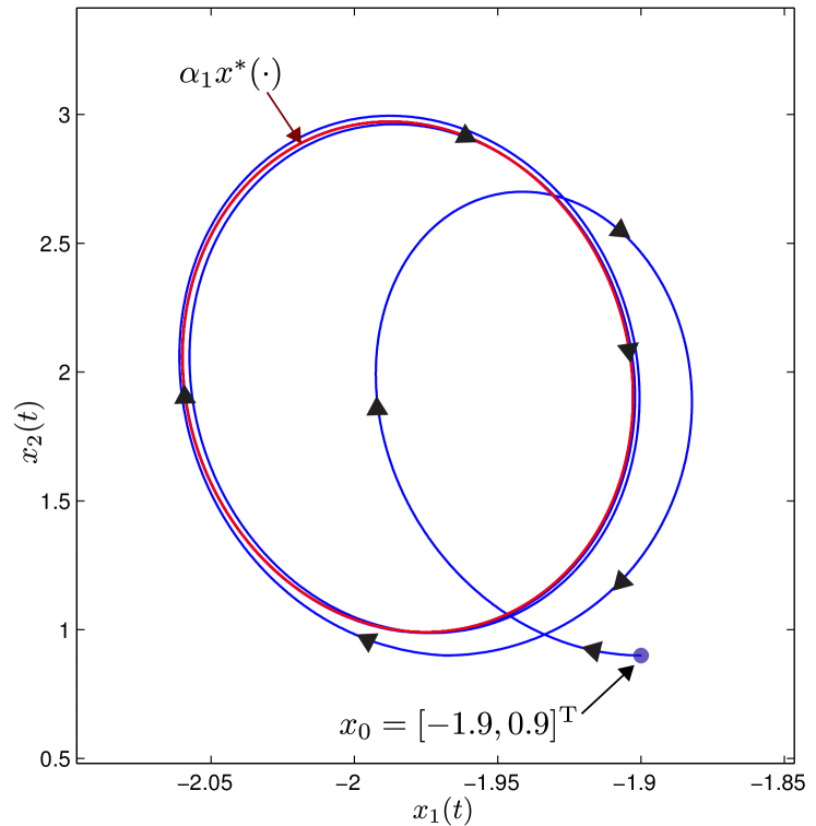
Figure 3: Phase portrait of the closed-loop system (1), (2) obtained with the initial condition $x_{0}=\left[-1.9,\,0.9\right]^{\mathrm{T}}$

\psfrag{x1}[bc]{\hskip 5.69046pt\footnotesize{$x_{1}(t)$}}\psfrag{x2}[bc]{\footnotesize{$x_{2}(t)$}}\psfrag{x1ttt}{\scriptsize{$x_{1}(t)$}}\psfrag{x2ttt}{\scriptsize{$x_{2}(t)$}}\psfrag{a1xstar1ttt}{\scriptsize{$\alpha_{1}x^{*}_{1}(t)$}}\psfrag{a1xstar2ttt}{\scriptsize{$\alpha_{1}x^{*}_{2}(t)$}}\psfrag{tt}[c]{\footnotesize{$\mathrm{Time}\,[t]$}}\includegraphics[width=390.25534pt]{controlled_x0_-1_9_09_x_with_alpha1xstar}

Figure 4: State trajectories of the closed-loop system (1), (2) obtained with the initial condition $x_{0}=\left[-1.9,\,0.9\right]^{\mathrm{T}}$

\psfrag{uu}[c]{\footnotesize{$u(t)$}}\psfrag{tt}[c]{\footnotesize{$\mathrm{Time}\,[t]$}}\includegraphics[width=390.25534pt]{controlled_x0_-1_9_09_u}

Figure 5: Control input versus time

Example 4.1 Consider the linear time-varying periodic system (1) described by periodic matrices

$$A(t) \triangleq\left[\begin{array}[]{cc}0.5&0.5\\ 0&\frac{2\pi\sin(2\pi t)}{2-\cos(2\pi t)}\end{array}\right],\,\,\,B(t)\triangleq\left[\begin{array}[]{c}0\\ 1+\sin^{2}(2\pi t)\end{array}\right].$$

The period of the time-varying system is $T=1$, that is, $A(t+1)=A(t)$ and $B(t+1)=B(t)$. The uncontrolled ($u(t)\equiv 0$) dynamics possess a $T$-periodic solution $x(t)\equiv x^{*}(t)$ given by

$$x^{*}(t)\triangleq\left[\begin{array}[]{c}\frac{1}{(1+16\pi^{2})}(\cos(2\pi t)-4\pi\sin(2\pi t))-2\\ 2-\cos(2\pi t)\end{array}\right].$$ (40)

Note that $x(t)\equiv\alpha x^{*}(t)$, where $\alpha\in\mathbb{R}$, is also a $T$-periodic solution of the uncontrolled system, that is, $x(t)\equiv\alpha x^{*}(t)$ satisfies (1) with $u(t)\equiv 0$. Fig. 1 shows the trajectory of the periodic solution $x(t)\equiv x^{*}(t)$.

The monodromy matrix associated with the uncontrolled system is given by

$$\Phi(T,0) =\left[\begin{array}[]{cc}1.6487&1.2934\\ 0&1\end{array}\right],$$ (43)

which has the eigenvalues $1.6487$ and $1$. Note that the eigenvalue $1.6487$ of the monodromy matrix $\Phi(T,0)$ lies outside the unit circle. The periodic system without control input, hence, shows unstable behavior (see Figure 2 for state trajectories obtained for the initial condition $x_{0}=\left[-1.9,\,0.9\right]^{\mathrm{T}}$).

We are interested in finding a feedback gain matrix $F\in\mathbb{R}^{1\times 2}$ such that the delayed-feedback control characterized in (2) guarantees convergence of the state trajectory towards a periodic solution. In order to evaluate the asymptotic behavior of solutions under the control law (2) we need to examine the eigenvalues of the monodromy matrix $\Lambda$ associated with the closed-loop system. It is difficult to find an analytical expression for the monodromy matrix $\Lambda$. For that reason, we numerically calculate the value of $\Lambda$ for a certain range of feedback gain parameters and search for a feedback gain matrix $F\in\mathbb{R}^{1\times 2}$ that satisfies the condition in Theorem 2.1. Note that for the feedback gain matrix $F=[4.5,\,\,0.6]$, the corresponding monodromy matrix is given by

$$\Lambda =\left[\begin{array}[]{cc}1.6857&1.3671\\ -0.8273&-0.6495\end{array}\right],$$ (46)

which has the eigenvalues $\lambda_{1}=1$ and $\lambda_{2}=0.0362$ associated with the eigenvectors $v_{1}=x^{*}(0)=[-1.9937,\,1]^{\mathrm{T}}$ and $v_{2}=[-0.6381,\,0.7699]^{\mathrm{T}}$, respectively. Note that the eigenvalue $\lambda_{2}$ is inside the unit circle of the complex plane. Therefore, it follows from Theorem 2.1 that under the control law (2), the state trajectory evaluated at integer multiples of the doubled period $2T$ converges to $\alpha_{1}v_{1}$, where $\alpha_{1}v_{1}$ represents the component of a given initial condition $x_{0}$ along the eigenvector $v_{1}=x^{*}(0)$. Figures 3 and 4 respectively show the phase portrait and state trajectories of the closed-loop system (1), (2) for the initial condition $x_{0}=[-1.9,\,0.9]^{\mathrm{T}}$, which can be represented as $x_{0}=\alpha_{1}v_{1}+\alpha_{2}v_{2}$ where $\alpha_{1}=0.9907$ and $\alpha_{2}=-0.1178$. Note that $\lim_{k\to\infty}x(2kT)=\alpha_{1}v_{1}=\alpha_{1}x^{*}(0)$ and hence the state trajectory converges to the periodic solution $\alpha_{1}x^{*}(t)$. Note that the convergence is achieved with the help of the proposed delayed feedback controller, which is turned on and off alternately at every integer multiples of the period $T=1$ of the uncontrolled system, and hence the control input (shown in Figure 5) is discontinuous at time instants $T$, $2T$, $3T$, $\ldots$. Note also that the control input converges to $0$ as the state converges to the periodic solution.

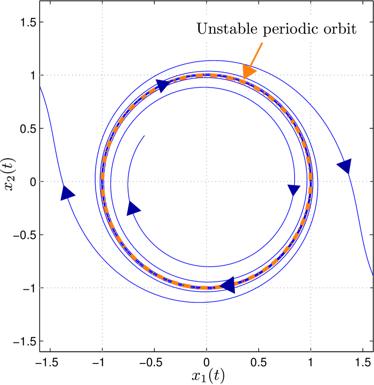
Figure 6: Phase portrait of the uncontrolled ($u(t)\equiv 0$) nonlinear system (27)

Example 4.2 In this example we demonstrate the utility of our proposed control framework for the stabilization of an unstable periodic orbit of a nonlinear system. Specifically, we consider the nonlinear dynamical system (27) with

$$f(x) \triangleq\left[\begin{array}[]{c}-x_{1}\big{(}\varphi(x)-\varphi^{2}(x)\big{)}+2\pi x_{2}\\ -x_{2}\big{(}\varphi(x)-\varphi^{2}(x)\big{)}-2\pi x_{1}\end{array}\right],$$ (49)

where $\varphi(x)\triangleq x_{1}^{2}+x_{2}^{2}$. This system is a modified version of an example nonlinear dynamical system considered in Section 2.7 of [28]. The phase portrait of the uncontrolled ($u(t)\equiv 0$) nonlinear system (27) is shown in Figure 6. The system has clockwise-revolving unstable periodic orbit $\mathcal{O}\triangleq\{x^{*}(t)\colon t\in[0,T)\}$, where $x^{*}(t)=[\cos 2\pi t,\,-\sin 2\pi t]^{\mathrm{T}}$ is a $1$-periodic solution of the uncontrolled system. The linear variational equation associated with the closed-loop system (27) under our proposed controller (2) (with $T=1$) is given by (33), where

$$A(t) =\left[\begin{array}[]{cc}a_{1,1}(t)&a_{1,2}(t)\\ a_{2,1}(t)&a_{2,2}(t)\end{array}\right]$$ (52)

with

$$a_{1,1}(t) =2\cos^{2}(2\pi t),$$ (53)

$$a_{1,2}(t) =-2\cos(2\pi t)\sin(2\pi t)+2\pi,$$ (54)

$$a_{2,1}(t) =-2\cos(2\pi t)\sin(2\pi t)-2\pi,$$ (55)

$$a_{2,2}(t) =2\sin^{2}(2\pi t).$$ (56)

Note that it is difficult to find an analytical expression for the monodromy matrix $\Lambda$ associated with the linear variational equation (33). For this reason, we numerically calculate the value of $\Lambda$ for a certain range of the elements of the gain matrix. In particular, for the case

$$F =\left[\begin{array}[]{cc}0.7&\,\,4.1\\ -4.1&\,\,0.7\end{array}\right],$$ (59)

the corresponding monodromy matrix is given by

$$\Lambda =\left[\begin{array}[]{cc}-0.0093&\,\,0\\ -6.5898&\,\,1\end{array}\right],$$ (62)

which has the eigenvalues $\lambda_{1}=-0.0093$, $\lambda_{2}=1$, and eigenvectors $v_{1}=[-0.1514,\,-0.9885]^{\mathrm{T}}$, $v_{2}=[0,\,-1]^{\mathrm{T}}$. Note that the eigenvalue $\lambda_{1}$ (eigenvalue that is not $1$) is inside the unit circle. Therefore, the feedback control law (2) with the feedback gain matrix (59) asymptotically stabilizes the periodic orbit $x^{*}(\cdot)$ of the nonlinear system (27) (see Remark 3.2).

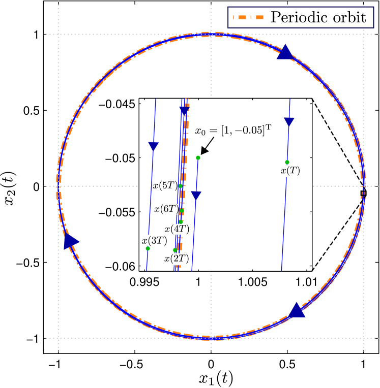
Figure 7: Phase portrait of the closed-loop system (2), (27). Inset figure shows the initial condition $x_{0}=[1,-0.05]^{\mathrm{T}}$ as well as the state evaluated at integer multiples of $T$.

Figures 7 and 8 respectively show the phase portrait and the state magnitude of the closed-loop system (2), (27) obtained for the initial condition $x_{0}=[1,-0.05]^{\mathrm{T}}$. The state trajectory converges to the periodic orbit and the state magnitude $\|x(t)\|$ converges to the desired value $1$.

Note that in this paper, we investigate local stability of the periodic orbit of the nonlinear system through a linearization approach. The initial condition $x_{0}$ in the simulation is selected close to $x^{*}(0)$, so that $\delta x(t)$ (the state deviation from the periodic solution) remains small and the effect of higher-order terms in the variational equation (32) is negligible. Note that, if the initial state is far from the orbit, then the control law (2) with the feedback gain $F$ may no longer achieve stabilization, since the higher order terms in the variational equation may have strong effects on the state trajectory. For achieving global stabilization, the higher-order terms in (32) have to be taken into consideration for control design.

\psfrag{magx}[bc]{\footnotesize{$\|x(t)\|$}}\psfrag{tt}[c]{\footnotesize{$\mathrm{Time}\,[t]$}}\includegraphics[width=390.25534pt]{magx}

Figure 8: State magnitude versus time

\psfrag{uu1}[c]{\footnotesize{$u_{1}(t)$}}\psfrag{uu2}[c]{\footnotesize{$u_{2}(t)$}}\psfrag{tt}[c]{\footnotesize{$\mathrm{Time}\,[t]$}}\includegraphics[width=390.25534pt]{u}

Figure 9: Control input versus time

The control input trajectory (shown in Figure 9) is discontinuous at time instants $T,2T,3T,\ldots$. At these time instants, the delayed-feedback controller is turned on and off alternately according to the switching function $g(t)$ defined in (5). For the $2T$-periodic switching function $g(t)$, the closed-loop system is $2T$-periodic; hence, the stabilization of the UPO could be characterized through the monodromy matrix $\Lambda$ of the $2T$-periodic closed-loop linear variational equation (33).

Note that stabilization of the UPO could also be achieved through utilization of alternative switching sequences that are different from the one induced by $g(t)$. For example, one can consider the switching function

$$\hat{g}(t) \triangleq\left\{\begin{array}[]{rl}0,&3kT\leq t<(3k+1)T,\\ 1,&(3k+1)T\leq t<3(k+1)T,\end{array}\right.\,k\in\mathbb{N}_{0}.$$ (65)

In this case the act-and-wait fashioned control law is given by

$$u(t) \triangleq-\hat{g}(t)F(x(t)-x(t-T)).$$ (66)

Note that the closed-loop system under the controller (66) is $3T$-periodic, thus by analyzing the spectrum of the monodromy matrix associated with the $3T$-periodic closed-loop linear variational equation, we can assess whether the control law (66) guarantees local asymptotic stabilization of the UPO or not.

According to the switching sequence induced by $\hat{g}(t)$, the controller is active two-thirds of the time in average. On the other hand, in the case of $g(t)$ defined in (5), the controller is active only half of the time. Hence, one may think that a feedback gain matrix that guarantees stabilization of the UPO for the case of $g(t)$ guarantees stabilization also for the case of $\hat{g}(t)$. However, this is not true. A feedback gain that guarantees stabilization for one switching sequence does not necessarily guarantee stabilization for another. For instance, the control input (2) with the gain matrix $F$ given by (59) achieves stabilization (as illustrated in Figures 7 and 8), whereas the control input (66) with the same gain matrix $F$ does not stabilize the UPO. In fact, the monodromy matrix of the $3T$-periodic closed-loop linear variational equation under the control law (66) possesses the eigenvalue $-25.9876$, which is outside the unit circle.

In addition to utilizing a different switching sequence for the act-and-wait controller, we may also employ a different delay term for the feedback for stabilizing the UPO. For example, consider the act-and-wait fashioned control law

$$u(t) \triangleq-\bar{g}(t)F(x(t)-x(t-2T)),$$ (67)

with the switching function

$$\bar{g}(t) \triangleq\left\{\begin{array}[]{rl}0,&4kT\leq t<(4k+2)T,\\ 1,&(4k+2)T\leq t<4(k+1)T,\end{array}\right.\,k\in\mathbb{N}_{0}.$$ (70)

Note that in this case the control law (67) harnesses the difference between the state at time $t$ (current state) and the state at time $t-2T$. Furthermore, with the switching function $\bar{g}(t)$, the controller is turned on and off alternately at time instants $2T,4T,6T,\ldots$. The closed-loop system under the control law (67) is $4T$-periodic. It is important to note here that the control input (67) with a feedback gain $F$ does not necessarily achieve stabilization of the UPO, even if the control law (2) with the same feedback gain guarantees stabilization. For example, with the feedback gain (59), the control law (2) achieves stabilization of the UPO, whereas the control law (67) does not. In fact, the monodromy matrix of the linear variational equation associated with the $4T$-periodic closed-loop system under the control law (67) with the feedback gain (59) has the eigenvalue $69.4489$, which is outside the unit circle. The discussion above illustrates that it is possible to obtain different control laws by changing the act-and-wait sequence and/or changing the delayed-feedback term; furthermore, each case with a different control law requires independent analysis for assessing asymptotic stabilization of the UPO.

In practical implementations of our act-and-wait-fashioned control laws, the timing of the switching may not always be exact. Furthermore, it may also be the case that the delay time and the period of the orbit do not exactly match. The effects of such practical issues require further analysis. We note that for the standard delayed feedback control, the effect of mismatches between the delay time and the period of the orbit was analyzed in [11]. We also note that although the trajectories of the act-and-wait-fashioned control law has discontinuities, this does not cause a practical problem in the form of chattering, because the switching in the control law happens only periodically with a period that is an integer multiple of the period of the orbit to be stabilized.

5 Conclusion

We explored stabilization of the periodic orbits of linear periodic time-varying systems through an act-and-wait-fashioned delayed feedback control framework. Our proposed framework employs a switching mechanism to turn the control input on and off alternately at every integer multiples of the period of the desired orbit. The use of this mechanism allows us to derive the monodromy matrix associated with the closed-loop dynamics. By analyzing the eigenvalues of the monodromy matrix, we obtained conditions under which the state trajectory converges towards a periodic solution. We then applied our results in stabilization of unstable periodic orbits of nonlinear systems. We discussed alternative switching sequences for turning the controller on and off in our control framework. We observe that a feedback gain that guarantees stabilization for one switching sequence does not necessarily guarantee stabilization for another. It is also interesting to observe that increasing the amount of time the control input is turned on does not necessarily increase the performance; in fact it may result in instability.

In the act-and-wait-fashioned control laws that we considered, the waiting duration where the control input is turned off is larger than or equal to the delay amount. It is shown in [29] that the act-and-wait approach can also be useful in obtaining finite-dimensional monodromy matrices even if the waiting duration is smaller than the delay. One of our future research directions is to investigate the utility of small waiting and acting durations in the delayed feedback control of periodic orbits.

References

- [1] K. Pyragas, Continuous control of chaos by self-controlling feedback, Phys. Lett. A 170 (1992) 421–428.
- [2] I. Harrington, J. E. S. Socolar, Design and robustness of delayed feedback controllers for discrete systems, Phys. Rev. E 69 (2004) 056207.
- [3] Y. Tian, J. Zhu, G. Chen, A survey on delayed feedback control of chaos, J. Control Theo. Appl. 3 (4) (2005) 311–319.
- [4] P. Hövel, Control of Complex Nonlinear Systems with Delay, Springer-Verlag: Berlin, 2010.
- [5] V. Pyragas, K. Pyragas, Adaptive search for the optimal feedback gain of time-delayed feedback controlled systems in the presence of noise, Eur. Phys. J. B 86 (7) (2013).
- [6] B. Fiedler, S. M. Oliva, Delayed feedback control of a delay equation at Hopf bifurcation, J. Dyn. Differ. Equ. 28 (3-4) (2016) 1357–1391.
- [7] N. Ichinose, M. Komuro, Delayed feedback control and phase reduction of unstable quasi-periodic orbits, Chaos 24 (3) (2014) 033137.
- [8] V. Pyragas, K. Pyragas, Relation between the extended time-delayed feedback control algorithm and the method of harmonic oscillators, Phys. Rev. E 92 (2) (2015) 022925.
- [9] A. A. Olyaei, C. Wu, Controlling chaos using a system of harmonic oscillators, Phys. Rev. E 91 (1) (2015) 012920.
- [10] V. Novičenko, K. Pyragas, Phase-reduction-theory-based treatment of extended delayed feedback control algorithm in the presence of a small time delay mismatch, Phys. Rev. E 86 (2) (2012) 026204.
- [11] A. S. Purewal, C. M. Postlethwaite, B. Krauskopf, Effect of delay mismatch in Pyragas feedback control, Phys. Rev. E 90 (5) (2014) 052905.
- [12] H. Ma, V. Deshmukh, E. Butcher, V. Averina, Controller design for linear time-periodic delay systems via a symbolic approach, in: Proc. Amer. Contr. Conf., 2003, pp. 2126–2131.
- [13] E. A. Butcher, H. Ma, E. Bueler, V. Averina, Z. Szabo, Stability of linear time-periodic delay-differential equations via Chebyshev polynomials, Int. J. Numer. Meth. Engng. 59 (2004) 895–922.
- [14] T. Insperger, Act-and-wait concept for continuous-time control systems with feedback delay, IEEE Trans. Contr. Sys. Tech. 14 (5) (2006) 974–977.
- [15] T. Insperger, G. Stepan, Act-and-wait control concept for discrete-time systems with feedback delay, IET Cont. Theory Applications 1 (3) (2007) 553–557.
- [16] T. Insperger, L. Kovacs, P. Galambos, G. Stepan, Increasing the accuracy of digital force control process using the act-and-wait concept, IEEE/ASME Trans. Mechatronics 15 (2) (2010) 291–298.
- [17] K. Konishi, H. Kokame, N. Hara, Delayed feedback control based on the act-and-wait concept, Nonlinear Dynamics 63 (3) (2011) 513–519.
- [18] V. Pyragas, K. Pyragas, Act-and-wait time-delayed feedback control of nonautonomous systems, Phys. Rev. E 94 (1) (2016) 012201.
- [19] P. Montagnier, R. J. Spiteri, A Gramian-based controller for linear periodic systems, IEEE Trans. Autom. Contr. 49 (8) (2004) 1380–1385.
- [20] B. Zhou, G.-R. Duan, Periodic Lyapunov equation based approaches to the stabilization of continuous-time periodic linear systems, IEEE Trans. Autom. Contr. 57 (8) (2012) 2139–2146.
- [21] C. E. De Souza, A. Trofino, An LMI approach to stabilization of linear discrete-time periodic systems, Int. J. Contr. 73 (8) (2000) 696–703.
- [22] M. A. F. Mohd Taib, T. Hayakawa, A. Cetinkaya, Delayed feedback control for linear time-varying periodic systems in act-and-wait fashion, in: Proc. 5th IFAC Int. Workshop on Periodic Control Systems, 2013, pp. 11–16.
- [23] D. Bernstein, Matrix Mathematics: Theory, Facts, and Formulas, Princeton University Press: Princeton, 2011.
- [24] J. Guckenheimer, P. Holmes, Nonlinear Oscillations, Dynamical Systems, and Bifurcations of Vector Fields, Springer: New York, 2002.
- [25] C. Chicone, Ordinary Differential Equations with Applications, Springer: New York, 2006.
- [26] R. Leine, H. Nijmeijer, Dynamics and Bifurcations of Non-Smooth Mechanical Systems, Springer-Verlag: Berlin, 2013.
- [27] L. Meirovitch, Methods of Analytical Dynamics, Dover: New York, 2003.
- [28] H. K. Khalil, Nonlinear Systems, Prentice Hall: New Jersey, 2002.
- [29] T. Insperger, G. Stepan, On the dimension reduction of systems with feedback delay by act-and-wait control, IMA J. Math Contr. Inform. 27 (2011) 457–473.