Vehicle Routing with Subtours

Abstract

When delivering items to a set of destinations, one can save time and cost by passing a subset to a sub-contractor at any point en route. We consider a model where a set of items are initially loaded in one vehicle and should be distributed before a given deadline $\Delta$. In addition to travel time and time for deliveries, we assume that there is a fixed delay for handing over an item from one vehicle to another.

We will show that it is easy to decide whether an instance is feasible, i.e., whether it is possible to deliver all items before the deadline $\Delta$. We then consider computing a feasible tour of minimum cost, where we incur a cost per unit distance traveled by the vehicles, and a setup cost for every used vehicle. Our problem arises in practical applications and generalizes classical problems such as shallow-light trees and the bounded-latency problem.

Our main result is a polynomial-time algorithm that, for any given $\epsilon>0$ and any feasible instance, computes a solution that delivers all items before time $(1+\epsilon)\Delta$ and has cost $\mathcal{O}(1+\frac{1}{\epsilon})\mbox{$\small\mathrm{OPT}$}$, where $\small\mathrm{OPT}$ is the minimum cost of any feasible solution.

Known algorithms for special cases begin with a cheap solution and decompose it where the deadline is violated. This alone is insufficient for our problem. Instead, we also need a fast solution to start with, and a key feature of our algorithm is a careful combination of cheap and fast solutions. We show that our result is best possible in the sense that any improvement would lead to progress on 25-year-old questions on shallow-light trees.

1 Introduction

Logistics companies are exploring innovative ways of delivering items to customers. In particular with an increasing number of crowdsourced delivery startups [19] comes new flexibility in designing delivery routes; e.g., [12] studies delivery applications where crowdsourcing is used to facilitate last-leg delivery of items. In the classical setting, a set of vehicles are initially located at a central depot that in turn serves as the starting point for all tours serving customers. Where deadlines are tight, this model naturally leads to a large number of tours, and implementing these solutions necessitates the maintenance of large vehicle fleets.

Our work is motivated by instances where the depot is relatively far from many customers. In designing delivery schedules, one would therefore want to use bigger vehicles to transport a large set of items closer to clusters of customers at which point one would then utilize smaller vehicles for the final leg of the delivery process. To model this situation, we introduce a new kind of vehicle routing problem and study its approximability.

Let us assume that a set of items is initially loaded on one vehicle and that they need to be delivered to their destinations by a given deadline $\Delta$. The vehicle can deliver items itself, but it can also – at any place en route – hand over a subset of its items to another vehicle. This vehicle can then deliver these items or can again hand over subsets to new vehicles en route.

Besides the normal travel cost per unit distance, we assume a fixed setup cost for every vehicle that we use. This assumption is of course a simplification, but some companies have vehicles at many different locations (almost everywhere) or hire sub-contractors that are not paid for their way to the meeting point where items are handed over to him. For the same reason, the way back home is not paid; therefore our tours are paths and not circuits. We remark that essentially the same problem arises when collecting items (or students) and transporting them to a central location (or school). However, to avoid confusion, we will speak of the delivery problem only.

We do not consider vehicle capacities here, although implicitly the number of items that a vehicle can handle is bounded by the deadline. We not only account for the travel time and the time to deliver items, but also consider a hand-over time proportional to the number of items exchanged.

Assuming that items can only be handed over from a vehicle to one other vehicle simultaneously, then the resulting route structure can best be described as an arborescence with maximum out-degree two, where the root corresponds to the starting point of the initial vehicle, vertices with out-degree two correspond to a hand-over, and all other vertices correspond to a delivery. We note that the imposed bound on the out-degree of our vertices is not restrictive, as we allow placing multiple vertices of the arborescence at the same geographical location.

1.1 Problem definition

Let us now describe the problem formally and introduce our notation. An instance consists of a finite set $P$ of item destinations, a root $r\notin P$, and a metric space $(M,c)$. We are also given a map $\mu:\{r\}\cup P\to M$ that assigns root and items in $P$ to locations in the metric space. Finally, we are given non-negative parameters $\delta$, $\sigma$ and $\Delta$, capturing delivery time, setup cost, and deadline, respectively.

We represent a schedule by an arborescence $(W,A)$ rooted at $r$ with $P\subset W$ and $\mu:W\setminus(P\cup\{r\})\to M$. An arc $(x,y)\in A$ means that a vehicle travels from $x$ to $y$, causing delay $c(\mu(x),\mu(y))$. At a vertex $p\in P$ we deliver the item $p$ and incur delay $\delta$. At a vertex $w\in W\setminus P$ with out-degree 2 we split off a subtour and incur a hand-over delay equal to the number of items handed over. Note that it is always better to hand over at most half of the items that are currently in the vehicle. We disallow out-degree greater than 2 because we need to specify the order of hand-overs. Assuming that a vehicle cannot simultaneously be involved in a delivery and a hand-over, we also forbid out-degree 2 for vertices in $P$. However, we allow that multiple vertices are mapped to the same point in the metric space, so multiple subtours can start at the same point in the metric space. A schedule allows that items are handed over multiple times on their path from the root to their destination.

The delay of a schedule is the maximum delay to an item. The cost of a schedule is $c(A,\mu)+s(W,A)$, where $c(A,\mu):=\sum_{(x,y)\in A}c(\mu(x),\mu(y))$ is the travel cost and $s(W,A):=\sigma\cdot|W_{0}|$ is the setup cost for vehicles; here $W_{0}$ denotes the set of leaves in $(W,A)$. The goal is to find a minimum-cost schedule with delay at most $\Delta$.

Figure 1: Example of a schedule. Edges are labeled by their distance (green). Vertices are labeled by hand-over delay (blue) or delivery delay (red, $\delta=4$). The initial vehicle delivers $p_{1}$, $p_{2}$ and $p_{3}$. It hands over parcels $p_{4}$, $p_{5}$ and $p_{6}$ to a second vehicle and later $p_{7}$ to a third vehicle. The second vehicle hands over $p_{6}$ to a fourth vehicle en route. The delay of this schedule is $30$ (attained at $p_{3}$). Its cost is $23+4\sigma$.

Figure 1 shows an example with seven items and a schedule with four vehicles.

1.2 Overview of results and techniques

As we will see in Section 1.4, our problem is a common generalization of several problems studied in the literature, including shallow-light trees and the bounded-latency problem. However, the possibility of starting subtours far away from the root and the handover delays make the problem more difficult.

Many previous approaches for special cases and similar problems, including the best-known algorithms for shallow-light trees and the bounded-latency problem (cf. Section 1.4), begin with a cheap solution (minimum spanning tree or short TSP tour), traverse it, and split the tree or tour whenever necessary to make the solution fast enough, connecting the next vertex directly to the root. However, this approach fails for our problem because connecting to the root can be too expensive and the order in which we split off subtours matters due to the handover delays.

We still use this tour-splitting technique to group the items, but in addition we need to begin with a fast solution. Therefore we first show that there always exists a fastest schedule with caterpillar structure, i.e., where all deliveries occur at leaves and the subgraph induced by the vertices with out-degree 2 is a path. As a corollary, one can easily compute such a solution and check whether a given instance is feasible (cf. Section 2).

In Section 3 we describe our algorithm. It first uses the tour-splitting technique to partition the items into groups each of which is spanned by a short path and does not contain too many items. Next, our algorithm constructs a two-level caterpillar so that items in the same group are consecutive, without violating the deadline much. Although this helps saving length, this schedule still uses a separate vehicle for every item and thus is usually very expensive. In a final step, we cluster subsets of groups to reduce the number of vehicles.

We compare our solution to a lower bound, composed of the length of a minimum cost tree spanning $\{r\}\cup P$ (in the following denoted by $\small\mathrm{MST}$) and a lower bound on the number of required vehicles. This will yield our main result:

Theorem 1.

Given a feasible instance and $\epsilon>0$, we can compute a solution with delay at most $(1+\epsilon)\Delta$ and cost $\mathcal{O}(1+\frac{1}{\epsilon})\mbox{$\small\mathrm{OPT}$}$ in polynomial time, where $\small\mathrm{OPT}$ is the minimum cost of a feasible schedule.

In Section 4 we will give an example that the tradeoff in Theorem 1 is unavoidable unless we use a significantly stronger lower bound. In fact, the example also shows that the 25-year old result of Cong et al. [4] on shallow-light trees is best possible. Since this is a special case of our problem, improving the dependency on $\epsilon$ by more than a constant factor would require new lower bounds for shallow-light trees and immediately lead to progress on this very well-studied problem.

1.3 Comments on our model

Before we move on, let us comment on two subtle assumptions that we made in our model, and argue why they are reasonable and necessary to obtain such a result.

First, we assume $\delta\geq 1$, that is, delivering an item to its final destination takes at least as long as handing it over to another vehicle (we assumed the hand-over time to be 1 per item, which is of course no loss of generality by scaling). This is certainly realistic in practice. Some assumption on $\delta$ is also necessary for our main result: with $\delta=0$, there is no polynomial-time algorithm delivering all items of a feasible instance before time $(1+\epsilon)\Delta$ for arbitrary small $\epsilon>0$ (unless $\mbox{P}=\mbox{NP}$). To see this, scale down the distances so that the shortest path beginning in $\mu(r)$ and containing $\mu(p)$ for all $p\in P$ has length less than 1. Then the earliest deadline that we can meet is the length of a shortest such path. However, determining this length is APX-hard (by straightforward reduction from the classical TSP [18]; cf. Appendix A).

Another subtle point in our model is that we pay $\sigma$ for every vehicle, including the initial one. Again, this looks reasonable from the practical point of view, although one might also think of the setup cost of the initial vehicle as already paid. But this assumption too is necessary for our main result. If we had assumed the initial vehicle to be free, then a very large value of $\sigma$ would force any reasonably cheap solution to be a path, and finding a path almost meeting a deadline is then equivalent to finding an almost shortest tour starting at $r$ and visiting all item destinations. As above, this problem is APX-hard.

Finally, our tours and subtours are paths rather than circuits. This is not very important though, because if every vehicle had to return to its starting point, the cost can at most double.

1.4 Related work

The problem discussed in this paper generalizes several well-studied, classical network design problems. For example, our problem contains the Steiner tree problem (set $\sigma=0$ and $\Delta=\infty$) and is thus APX-hard [3].

An interesting special case of our problem arises when $\sigma=0$ and $c$ is large compared to $\delta$. In other words, the traveled distance dominates the delay and the cost of any schedule. In this case, the goal would be to compute a Steiner tree (or if $M=\mu(\{r\}\cup P)$ a spanning tree) that balances cost and the maximum distance from the root.

Awerbuch et al. [2] first showed that every finite metric space contains a spanning tree whose diameter is at most a constant times that of the underlying metric space, and whose weight is at most a constant times that of a minimum-cost spanning tree. Such trees are called shallow-light trees. Cong et al. [4] improved these results; they showed how to find, for any $\epsilon>0$, a spanning tree of length at most $(1+\frac{2}{\epsilon})\mbox{$\small\mathrm{MST}$}$ in which the path from $r$ to any other vertex is no longer than $1+\epsilon$ times the maximum distance from $r$. Khuller, Raghavachari and Young [15] generalized this work to obtain, for any $\epsilon>0$, a tree $T$ with total cost at most $(1+\frac{2}{\epsilon})\mbox{$\small\mathrm{MST}$}$ such that, for every $v\in P$, the distance in $T$ from $r$ to $v$ is at most $1+\epsilon$ times the distance between $r$ and $v$ in the metric space.

Khuller et al. [15] also gave an example showing that the obtained tradeoff is best possible. In Section 4 we generalize their example to prove that this is true even for instances where all vertices have the same distance from $r$; implying that the result of [4] on shallow-light trees is also best possible. This will also show that Theorem 1 is best possible unless we use a stronger lower bound than $\small\mathrm{MST}$.

A further generalization was given by Held and Rotter [9], considering Steiner trees and having an additional distance penalty per bifurcation. However, in all of the above algorithmic variants the result may have many leaves and the delay models differ substantially from hand-over delays in our model.

There has been a tremendous amount of work on solving optimization problems arising in the general context of vehicle routing, and we cannot provide an adequate survey here. We focus on the most closely related work that we are aware of, and refer the reader to Toth and Vigo’s book [20] for a more comprehensive introduction.

Another interesting special case of our problem arises when delays are dominated by travel times and cost is dominated by the setup cost. Then it does not harm to start all subtours at the position of the root, and the problem reduces to covering the items by as few paths as possible, each starting at the root and having length at most $\Delta$. Jothi and Raghavachari [11] called this problem the bounded-latency problem. They observed that the tour-splitting technique yields a solution violating the deadline by at most a factor of $(1+\epsilon)$ and using at most $\frac{2}{\epsilon}$ times the optimum number of paths.

A similar problem is the distance-constrained vehicle routing problem (DVRP), where the goal is to cover the items by a minimum number of closed tours (returning to the root), each having length at most $\Delta$. Khuller, Malekian, and Mestre [16] and independently Nagarajan and Ravi [17] gave an $(1+\epsilon,\mathcal{O}(\log\frac{1}{\epsilon}))$-bicriteria approximation algorithm. This also works for the bounded-latency problem: partition the items according to their distance from $r$: items at distance more than $(1-2\epsilon)\Delta$ are in group 1, and items at distance between $(1-2^{j}\epsilon)\Delta$ and $(1-2^{j-1}\epsilon)\Delta$ are in group $j$ ($j=2,\ldots,\lceil\log\frac{1}{\epsilon}\rceil$). Then each group $j$ is covered by (unrooted) paths, each of which has length at most $2^{j-1}\epsilon\Delta$ and can be completed by an edge to $r$, exceeding length $\Delta$ by at most $\epsilon\Delta$ (only in group 1). The number of these paths can be minimized up to a factor 3 using an algorithm of [1]. If $\small\mathrm{OPT}$ is the number of tours in an optimal solution, we can cover each group by $2\mbox{$\small\mathrm{OPT}$}$ paths (shortcutting those that contain at least one item this group and splitting it into two if necessary). Thus we end up with at most $6\mbox{$\small\mathrm{OPT}$}$ paths in each group, and $6\lceil\log\frac{1}{\epsilon}\rceil\mbox{$\small\mathrm{OPT}$}$ paths in total.

Connecting all paths to the root can, however, be much more expensive than splitting off subtours elsewhere: for instance, if all items are to be delivered at the same position far away from the root, and the (relaxed) deadline prevents any tour from delivering more than one item, then the total length increases by a factor $|P|$ if we insist that all paths start at the root. See also Appendix B for a similar example.

Friggstad and Swamy [6] studied regret-bounded variants of vehicle routing problems and provided an $\mathcal{O}(\log\Delta/\log\log\Delta)$ approximation for DVRP under the assumption that the minimum distance in the underlying metric is at least one. Gørtz et al. [8] considered various vehicle routing problems in the setting where vehicles have non-uniform speeds and capacities. Among other things, the authors study the variant of DVRP where the vehicles have finite capacity and non-uniform speeds, and where the goal is to minimize the deadline. Gørtz et al. provide a constant-factor approximation algorithm for this problem.

Closely related to DVRP are vehicle routing problems with min-max objective. A typical such problem is the min-max $X$-cover problem, where $X\in\{\mbox{path, tree, tour, }\ldots\}$. Here, one is given a metric space on $n$ points, and a parameter $k$, and the goal is now to find a collection of $k$ subgraphs of type $X$ to cover all points so that the maximum length of any of these subgraphs is smallest. The problem is APX-hard in the case of trees [21] and constant-factor approximation algorithms are known [1, 5, 14]. Xu, Xu and Li [22] study the min-max path cover problem and obtain constant-factor approximation algorithms for several variants, also including delivery times.

Another notable variant is the preemptive multi-vehicle dial-a-ride problem, where $n$ items have to be transported by a fixed number of vehicles, which are located at given depots. Item $i\in\{1,\dots,n\}$ has to be picked up at $s_{i}$ and delivered to $t_{i}$. Items may be passed from one vehicle to another on their journey. Gørtz, Nagarajan, and Ravi [7] present an $\mathcal{O}(\log^{3}n)$-approximation algorithm for minimizing the makespan under capacity constraints, and an $\mathcal{O}(\log t)$-approximation algorithm without vehicle capacities, where $t$ is the number of distinct depots.

2 Deciding Feasibility

2.1 Notation

Let us call an arborescence proper if its root is $r$ and has out-degree 1, all elements of $P$ are vertices with out-degree 0 or 1, and all other vertices have out-degree 2. We may restrict ourselves to schedules with proper arborescences because if the root has out-degree 2 we can introduce an extra vertex at the same location without changing delay or cost.

For a proper arborescence $(W,A)$ and $x\in W$ we use the following notation: $(W_{x*},A_{x*})$ is the maximal subarborescence of $(W,A)$ rooted at $x$. For $y\in W_{x*}$ we denote by $(W_{xy},A_{xy})$ the path from $x$ to $y$ in $(W,A)$. We have $W=W_{0}\cup W_{1}\cup W_{2}$, where $W_{i}$ contains the vertices of out-degree $i$ ($i=0,1,2$). The elements of $W_{0}$ are called leaves, and the elements of $W_{2}$ are the bifurcation nodes. Note that $|W_{0}|=|W_{2}|+1$.

With this notation, we extend the definition of delay of an item in a schedule $(W,A,\mu)$ to any vertex $y\in W$:

$${\mathrm{delay}}_{(W,A,\mu)}(r,y)\ :=\ c(A_{ry},\mu)\,+\,\delta|P\cap W_{ry}|\,+\!\sum_{w\in W_{ry}\cap W_{2}}\min_{(w,x)\in\delta^{+}(w)}|P\cap W_{x*}|.$$

The first term is the delay of traversing edges, the second term is the time for delivering items on the $r$-$y$-path, and the third term is the time to hand over a subset of items to a subtour. Now, the delay of a schedule $(W,A,\mu)$ can be written as

$${\mathrm{delay}}(W,A,\mu)\ :=\ \max_{p\in P}{\mathrm{delay}}_{(W,A,\mu)}(r,p).$$

We denote by $n:=|P|$ the number of items.

2.2 Caterpillar structure

If we disregard cost, we can afford a separate vehicle for every item, going straight from the root to the item’s destination. This certainly minimizes the first two components (travel time and delivery time) of the delay to each item. Then the only question is how the tree structure should look like, because it will determine the handover delays. It turns out that there is always a fastest solution with a caterpillar structure. This allows us to determine efficiently whether a feasible solution exists.

We first introduce the leafication step that takes a vertex with fanout one and branches it off as a single leaf.

Definition 2 (Leafication).

Consider a schedule $(W,A,\mu)$. Let $y\in W_{1}\setminus\{r\}$, and let $(x,y),(y,z)\in A$ be the two arcs incident to $y$ in $(W,A)$. The leafication of $y$ is the new schedule $(W^{\prime},A^{\prime},\mu^{\prime})$ with $W^{\prime}=W\dot{\cup}\{y^{\prime}\}$, where $y^{\prime}$ is a new vertex,

$$A^{\prime}\ =\ A\setminus\{(x,y),(y,z)\}\cup\left\{(x,y^{\prime}),(y^{\prime},y),(y^{\prime},z)\right\},$$

$\mu^{\prime}(u)=\mu(u)$ for all $u\in W$, and $\mu^{\prime}(y^{\prime})=\mu(y)$.

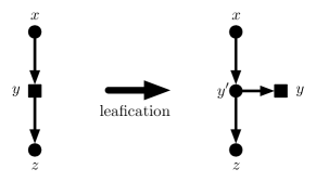
Figure 2: Leafication of $y$.

See Figure 2. The leafication does not increase the delay of the schedule:

Lemma 3.

If $(W^{\prime},A^{\prime},\mu^{\prime})$ is obtained from $(W,A,\mu)$ through a leafication, then

$${\mathrm{delay}}(W^{\prime},A^{\prime},\mu^{\prime})\ \leq\ {\mathrm{delay}}(W,A,\mu).$$

Proof: Let $y$ be the leafication vertex and $(x,y),(y,z)\in A$ its incident arcs. First note that the leafication changes delays only in $W_{y\star}=W^{\prime}_{z\star}\cup\{y\}$. Furthermore, $c(A_{rp},\mu)=c(A^{\prime}_{rp},\mu^{\prime})$ for all $p\in P$. Now for $y$ and any $w\in W_{z\star}\cap P$ we have

$$\begin{array}[]{rcl}{\mathrm{delay}}_{(W^{\prime},A^{\prime},\mu^{\prime})}(r,y)&\leq&{\mathrm{delay}}_{(W^{\prime},A^{\prime},\mu^{\prime})}(r,w)\\ &=&{\mathrm{delay}}_{(W,A,\mu)}(r,w)-\delta+1\\ &\leq&{\mathrm{delay}}_{(W,A,\mu)}(r,w)\\ &\leq&\displaystyle\max_{p\in P}{\mathrm{delay}}_{(W,A,\mu)}(r,p),\end{array}$$

where the first inequality follows from the fact that $w$ collects at least the handover delay as $y$ and at least its own delivery time. The equality follows from replacing the delivery time by the handover time for $y$ on the path to $z$. The second last inequality follows from $\delta\geq 1$. We conclude ${\mathrm{delay}}(W^{\prime},A^{\prime},\mu^{\prime})\leq{\mathrm{delay}}(W,A,\mu)$. $\Box$

By leafication we can get rid of out-degree 1 vertices (except for the root). In order to obtain the caterpillar structure we need to move all out-degree 2 vertices onto a single “heavy” path:

Definition 4 (Heavy path).

Given a proper arborescence $(W,A)$, a vertex $x\in W$ is called heavy if $x=r$ or $|W_{x*}\cap P|\geq|W_{y*}\cap P|$ for every child $y$ of the predecessor of $x$. A heavy path in $(W,A)$ is maximal set of heavy vertices that induce a path.

Note that any heavy path begins at the root and ends at a leaf. We will move all bifurcation nodes onto a heavy path by the following operation.

Definition 5 (Flip).

Consider a schedule $(W,A,\mu)$, and $H$ a heavy path in $(W,A)$. Let $w\in W_{2}\cap H$, and let $h$ be the child of $w$ that belongs to $H$. Suppose that the other child $x$ of $w$ is a bifurcation node with $\mu(h)=\mu(x)$. Let $y_{h}$ and $y_{l}$ be the two children of $x$, where $y_{h}$ is heavy. The flip at $x$ is the new schedule $(W,A^{\prime},\mu)$ with

$$A^{\prime}\ :=\ A\setminus\{(w,h),(x,y_{l})\}\cup\{(w,y_{l}),(x,h)\}.$$

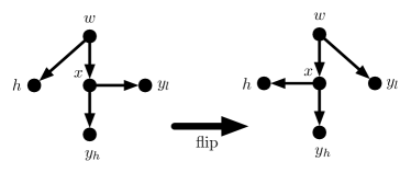
Figure 3: Flip operation.

See Figure 3. Note that $H\cup\{x\}$ is a heavy path in $(W,A^{\prime})$. We now show that a flip does not make a schedule slower.

Lemma 6.

If $(W,A^{\prime},\mu)$ is obtained from $(W,A,\mu)$ through a flip, then

$${\mathrm{delay}}(W^{\prime},A^{\prime},\mu^{\prime})\ \leq\ {\mathrm{delay}}(W,A,\mu).$$

Proof: First note that $c(A^{\prime}_{rp},\mu)\leq c(A_{rp},\mu^{\prime})$ for all $p\in P$ due to $\mu(h)=\mu(x)$ and the triangle inequality. We show that the total handover delay to any item does not increase. By construction the delays of items outside $W_{x*}$ coincide for $(W,A,\mu)$ and $(W,A^{\prime},\mu)$. The handover delays of the flipped schedule are reduced by $|W_{y_{l}*}\cap P|$ for all items in $W_{y_{h}*}$ and by $|W_{x*}\cap P|$ for all items in $W_{y_{l}*}$. $\Box$

In graph theory, caterpillars are trees for which deleting all leaves results in a path. We use the term for arborescences in a slightly different way:

Definition 7 (Caterpillar).

A proper arborescence $(W,A)$ is a caterpillar if $W_{1}=\{r\}$ and the subgraph induced by $\{r\}\cup W_{2}$ is a path. For $P=\{p_{1},\ldots,p_{n}\}$ we denote by $C(p_{n},\ldots,p_{1})$ the caterpillar in which the $r$-$p_{i}$-path in $(W,A)$ has $\min\{n,n+2-i\}$ edges for all $i=1,\ldots,n$.

See Figure 4. Now we can show the main result of this section.

Theorem 8.

There exists a schedule $(W,A,\mu)$ with minimum delay such that $(W,A)$ is a caterpillar and $\mu(w)=\mu(r)$ for all $w\in W_{2}$.

Proof: If $n=1$, the statement is clearly true, so let $n>1$. Let $(A^{0},W^{0},\mu^{0})$ be a schedule with minimum delay. Recall that $W^{0}_{0}\cup W^{0}_{1}=\{r\}\cup P$.

Step 1: By iteratively applying a leafication step to all $y\in W^{0}_{1}\setminus\{r\}$, we can transform it into a schedule $(A^{1},W^{1},\mu^{1})$ with $W^{1}_{1}=\{r\}$ that still has minimum delay. Then all items are delivered at leaves, i.e., $P=W^{1}_{0}$.

Step 2: We transform $(A^{1},W^{1},\mu^{1})$ into $(A^{2},W^{2},\mu^{2})$, by setting $A^{2}=A^{1},W^{2}=W^{1}$ and $\mu^{2}(y)=\mu^{1}(r)$ for all $y\in W^{2}_{2}$. As $(A^{1},W^{1})=(A^{2},W^{2})$, only the delays for traversing arcs change in $(A^{2},W^{2},\mu^{2})$. But as $c(A^{2}_{rp},\mu^{2})=c(r,p)$ for all $p\in P$, this part of the delay is minimum possible and so $(A^{2},W^{2},\mu^{2})$ still has minimum delay.

Step 3: Finally, we use the flip operation to obtain the caterpillar structure. Let $H$ be a heavy path. As long as there is a bifurcation node outside $H$, there is such a vertex $x$ such that its predecessor $w$ belongs to $H$. Then applying the flip operation at $x$ increases the cardinality of $H$ by one, so after finitely many steps, the heavy path contains all bifurcation nodes. $\Box$

2.3 Consequences

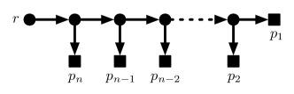
Figure 4: Caterpillar $C(p_{n},\ldots,p_{1})$.

Corollary 9.

For any feasible instance we have

1. $\Delta\geq\min\bigl{\{}c(r,q)+\delta+\min\{|Q|,n-1\}:q\in Q\bigr{\}}$ for every nonempty subset $Q\subseteq P$;

2. $\Delta\geq n$;

3. $\Delta\geq\max\{c(r,p):p\in P\}$.

Proof: For (a), let $Q\subseteq P$, and consider a feasible caterpillar (which exists by Theorem 8). At least one of the $|Q|$ items, say $q$, will have at least $\min\{|Q|,n-1\}$ bifurcation nodes on its path. The path to $q$ has length $c(r,q)$ and it also pays $\delta$ for delivering $q$.

(b) follows from (a) by setting $Q=P$ and using $\delta\geq 1$. (c) is obvious. $\Box$

Theorem 8 allows us to determine efficiently whether a feasible schedule exists.

Corollary 10.

We can find a schedule meeting the deadline or decide that none exists in time $\mathcal{O}(n\log n+\theta n)$, where $\theta$ is the time to evaluate distances in $(M,c)$.

Proof: If $n=1$, verifying the feasibility of the deadline is easy, so let $n>1$. By Theorem 8 there is a fastest solution $(A,W,\mu)$ such that $(A,W)$ is a caterpillar. This caterpillar is unique up to the order in which the items are attached as leaves. Furthermore, the distribution of total handover delays for the leaves is predetermined and each item suffers a single delivery delay of $\delta$ for its own delivery. So the leaves have delivery plus handoff delay $1+\delta,2+\delta,\ldots,n-2+\delta,n-1+\delta,n-1+\delta$.

Thus it suffices to find an assignment of the items to the leaves that meets the deadline. The best we can do is to iteratively assign an item with the maximum distance from $r$ to the closest available leaf in the arborescence. To this end we sort the items by their distance from $r$. Let $p_{1},p_{2},\dots,p_{n}$ be the ordering of the items by non-decreasing distance from $r$, i.e. $c(r,p_{i})\leq c(r,p_{i+1})$ for all $i\in\{1,\dots,n-1\}$.

We assign the items $p_{1},p_{2},\dots,p_{n}$ one by one to a not yet occupied leaf vertex that has a maximum number of arcs on its path from $r$ (cf. Figure 4). The deadline $\Delta$ can be met if and only if the generated schedule meets it.

The running time is dominated by sorting the items, which can be done in $\mathcal{O}(n\log n)$ time, and by computing all root to item distances, which takes $\theta\cdot n$ time. $\Box$

The schedule from Theorem 8 is fast but also expensive. It has the maximum possible setup cost of $\sigma\cdot n$ and also high travel costs, as each item is transported individually from the root location to its destination.

3 Algorithm

Our algorithm first groups the items by splitting a short tour into paths similar to [1]. The items in each group will have similar distance from $r$. Therefore, rearranging the fastest solution with the caterpillar structure (Theorem 8) so that the items in each group are consecutive does not make the schedule much slower. Next, we design a two-level caterpillar, where the items in each group are served by a caterpillar and the groups are served by a top-level caterpillar. In order to avoid that all subtours begin at the position of the root, we make the main tour of each sub-caterpillar drive to all locations of items in that group. Finally, we avoid too many subtours by merging tours in each subcaterpillar.

3.1 Grouping items

Lemma 11.

Let $\small\mathrm{MST}$ denote the length of a minimum cost tree with vertex set $\{r\}\cup P$, and let $s\in P$ be an item at maximum distance from $r$. Let $\epsilon>0$ and $0<\Delta\leq\mbox{$\small\mathrm{MST}$}$. Then there is a forest $(P,F)$ whose components are vertex-disjoint paths such that

1. the number of paths is at most $1+\frac{n+2\,\mbox{$\small\mathrm{MST}$}-c(r,s)}{\epsilon\Delta}$;

2. no path is longer than $\epsilon\Delta$;

3. no path contains more than $1+\epsilon\Delta$ items;

4. $c(F)\leq 2\,\mbox{$\small\mathrm{MST}$}-c(r,s)$.

Such a forest can be found in polynomial time.

Proof: Take any approximately cheapest path with vertex set $\{r\}\cup P$ from $r$ to $s$. We can find it by taking a minimum cost spanning tree for $\{r\}\cup P$ in $(M,c)$, doubling all edges except those of the $r$-$s$-path, finding an Eulerian $r$-$s$-walk, and shortcutting. The resulting $r$-$s$-path $(\{r\}\cup P,F_{0})$ has total cost at most $2\,\mbox{$\small\mathrm{MST}$}-c(r,s)$. From now on, we will only delete edges, yielding (d).

To satisfy (b) and (c), we start with $F=\emptyset$ and traverse the path $r$-$s$-path, ignoring $r$ and the first edge. In each step, we add the next edge to $F$ unless this would violate (b) or (c).

The conditions (b), (c), and (d) are then satisfied by construction. Whenever we drop an edge $e$, one of the conditions (b) and (c) would be violated for $P\cup\{e\}$, where $P$ is a connected component of $F$. If (b), the length of $P\cup\{e\}$ exceeds $\epsilon\Delta$, so this can happen at most $\frac{c(F_{0})}{\epsilon\Delta}$ times. If (c), the number of items in $P$ exceeds $\epsilon\Delta$, so this can happen at most $\frac{n}{\epsilon\Delta}$ times. So we drop at most $\frac{2\,\mbox{$\small\mathrm{MST}$}-c(r,s)}{\epsilon\Delta}+\frac{n}{\epsilon\Delta}$ edges (in addition to the initial one). This yields (a). $\Box$

Note that (b) immediately implies that items in the same path have similar distances from $r$: if $p$ and $p^{\prime}$ are in the same path, the triangle inequality yields $c(r,p)\leq c(r,p^{\prime})+\epsilon\Delta$.

3.2 Towards a cheaper schedule

Let us call the vertex sets of the connected components of $(P,F)$ from Lemma 11 groups; they form a partition of $P$. For $p\in P$, let

$$d(p):=\max\{c(r,p^{\prime}):\text{$p$ and $p^{\prime}$ are in the same group}\}$$

be the distance from $r$ to the most remote item in the same group as $p$ (note that $p^{\prime}=p$ is not excluded). Order the items $P=\{p_{1},\ldots,p_{n}\}$ such that

$$d(p_{1})\leq\cdots\leq d(p_{n})$$

and

$$F\subseteq\{\{p_{i},p_{i+1}\}:i=1,\ldots,n-1\},$$

so items of the same group are consecutive, every edge in $F$ connects two consecutive items, and groups containing more remote items come later.

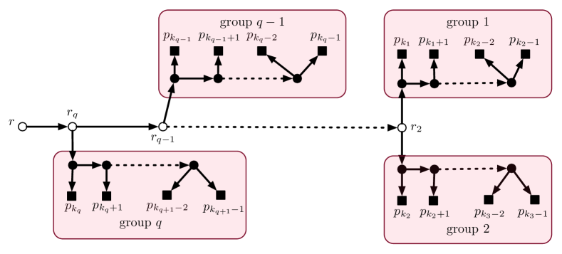
Figure 5: Schedule $S_{1}$ with a sub-caterpillar for each group.

Let $P=\{p_{1},\ldots,p_{n}\}$ be the items ordered as above, and let $1=k_{1}<k_{2}<\cdots<k_{q+1}=n+1$ such that $\{p_{k_{i}},\ldots,p_{k_{i+1}-1}\}$ ($i=1,\ldots,q$) are the groups. Let $S_{1}$ be the schedule resulting from a path with vertices $r,r_{q},r_{q-1},\ldots,r_{2}$ in this order by identifying the root of the caterpillar $C(p_{k_{i}},\ldots,p_{k_{i+1}-1})$ with $r_{\max\{2,i\}}$ ($i=1,\ldots,q$; see Figure 5). The bifurcation nodes $r_{q},\ldots,r_{2}$ are placed at $\mu(r)$, but the bifurcation nodes of the subcaterpillars are placed at the position of the item that splits off there: the $j$-th bifurcation node of the subcaterpillar for group $i$ is placed at $\mu(p_{k_{i}+j-1})$.

Lemma 12.

If the instance is feasible, then ${\mathrm{delay}}(S_{1})\leq(1+3\epsilon)\Delta$.

Proof: Consider group $i$ with items $p_{k_{i}},\ldots,p_{k_{i+1}-1}$. The maximum delay of an item in this group is the one to $p_{k_{i+1}-1}$, which is at most

$$c(r,p_{k_{i}})+\sum_{l=k_{i}}^{k_{i+1}-2}c(p_{l},p_{l+1})+n-k_{\max\{2,i\}}+1+k_{i+1}-k_{i}-1+\delta,$$

which by Lemma 11(b) and (c) is at most

$$d(p_{k_{i}})+\epsilon\Delta+n-k_{\max\{2,i\}}+1+\epsilon\Delta+\delta.$$ (1)

By Corollary 9 (a), there exists a $j\in\{k_{i},\ldots,n\}$ with $\Delta\geq c(r,p_{j})+n-\max\{2,k_{i}\}+1+\delta$.

Since $d(p_{k_{i}})\leq d(p_{j})\leq c(r,p_{j})+\epsilon\Delta$, we have

$$\Delta \geq c(r,p_{j})+n-\max\{2,k_{i}\}+1+\delta$$

$$\geq c(r,p_{j})+n-k_{\max\{2,i\}}+1+\delta$$

$$\geq d(p_{k_{i}})-\epsilon\Delta+n-k_{\max\{2,i\}}+1+\delta.$$

Hence our bound (1) on the maximum delay of an item in group $i$ yields that this delay is at most $(1+3\epsilon)\Delta$. $\Box$

We can bound the length of $S_{1}$ as follows:

Lemma 13.

$S_{1}$ has length at most $(2+\frac{2}{\epsilon})\mbox{$\small\mathrm{MST}$}$.

Proof: The length of the schedule is $\sum_{i=1}^{q}c(r,p_{k_{i}})$ (which is the initial edges of the sub-caterpillars) plus $c(F)$ (remaining length of the subcaterpillars). By Lemma 11, $c(F)\leq 2\,\mbox{$\small\mathrm{MST}$}-c(r,s)$ and the number $q$ of groups is at most $1+\frac{n+2\,\mbox{$\small\mathrm{MST}$}-c(r,s)}{\epsilon\Delta}$. Moreover $c(r,p_{k_{i}})\leq c(r,s)$ for all $i$ by the choice of $s$. Hence the length of the schedule is at most

$$q\,c(r,s)+2\,\mbox{$\small\mathrm{MST}$}-c(r,s)\leq\frac{n+2\,\mbox{$\small\mathrm{MST}$}-c(r,s)}{\epsilon\Delta}\,c(r,s)+2\,\mbox{$\small\mathrm{MST}$}.$$

Since $n\leq\Delta$ and $c(r,s)\leq\Delta$ by Corollary 9 (b) and (c), this is at most

$$\frac{\Delta}{\epsilon\Delta}c(r,s)+\frac{2\,\mbox{$\small\mathrm{MST}$}-c(r,s)}{\epsilon\Delta}\Delta+2\,\mbox{$\small\mathrm{MST}$}=\left(2+\frac{2}{\epsilon}\right)\,\mbox{$\small\mathrm{MST}$}.$$

$\Box$

3.3 Saving vehicles

The schedule is already short, but it still contains a separate vehicle for each item. However, we can deliver up to $m:=1+\lfloor\frac{\epsilon\Delta}{\delta}\rfloor$ items by the same vehicle by replacing the edge entering an item $p_{j}$ in group $i$ by the edge $(p_{j-1},p_{j})$ unless $j-k_{i}$ is a multiple of $m$. The resulting schedule $S_{2}$ is the output of our algorithm, except that we remove the non-item nodes that now have out-degree 1, by shortcutting.

Lemma 14.

$S_{2}$ has delay at most $(1+4\epsilon)\Delta$ and length at most $(4+\frac{2}{\epsilon})\mbox{$\small\mathrm{MST}$}$. It has at most $1+\frac{2}{\epsilon}\left(\frac{\mbox{$\small\mathrm{MST}$}+n\delta}{\Delta}\right)$ vehicles.

Proof: Going from $S_{1}$ to $S_{2}$ increases the maximum delay of an item in a group by at most $(m-1)\delta\leq\epsilon\Delta$, because the maximum travel time and the maximum handover delay in each group cannot increase.

The length of $S_{2}$ is at most $c(F)$ longer than $S_{1}$. Since $c(F)\leq 2\mbox{$\small\mathrm{MST}$}$, the length bound follows.

The total number of vehicles is at most

$$q+\frac{n}{m}\leq q+\frac{\delta n}{\epsilon\Delta}\leq 1+\frac{n+2\,\mbox{$\small\mathrm{MST}$}-c(r,s)}{\epsilon\Delta}+\frac{\delta n}{\epsilon\Delta}\leq 1+\frac{2}{\epsilon}\left(\frac{\mbox{$\small\mathrm{MST}$}+n\delta}{\Delta}\right),$$

where we used $\delta\geq 1$ in the last inequality. $\Box$

We compare this to the following lower bound.

Lemma 15.

Every feasible schedule has length at least $\frac{1}{2}\mbox{$\small\mathrm{MST}$}$ and uses at least $\frac{\frac{1}{2}\text{\scriptsize\mbox{$\small\mathrm{MST}$}}+n\delta}{\Delta}$ vehicles, where $\small\mathrm{MST}$ is the length of a minimum spanning tree for $\mu(\{r\}\cup P)$.

Proof: Any schedule connects $\{r\}\cup P$, so the lower bound $\frac{1}{2}\mbox{$\small\mathrm{MST}$}$ for the length follows from the Steiner ratio. For the bound on the number of vehicles, fix any feasible schedule $(W^{*},A^{*},\mu^{*})$, say with $l^{*}$ vehicles numbered $1,\ldots,l^{*}$. Let $D_{i}$ be the delay of the last item that vehicle $i$ delivers; this is at most $\Delta$. As each edge needs to be traversed and each item delivered by one of the vehicles,

$$\frac{1}{2}\mbox{$\small\mathrm{MST}$}+n\delta\ \leq\ c(A^{*},\mu^{*})+n\delta\ \leq\ \sum_{i=1}^{l^{*}}D_{i}\ \leq\ l^{*}\Delta.$$

$\Box$

Lemma 14 and 15 imply that the cost of our schedule is at most $8+\frac{4}{\epsilon}$ times the cost of an optimum schedule. This proves Theorem 1.

Our algorithm is very fast – the running time is dominated by computing a minimum spanning tree and sorting the groups.

We remark that the constants can be improved, for example by beginning with a Steiner tree that is a better approximation than MST. However, any improvement by more than a constant factor would imply an improvement over the 25-year old bicriteria algorithm for shallow-light trees by Cong et al. [4]. We will demonstrate this in the following.

4 An almost tight example

We now show that our bicriteria result is the best we can hope for up to constant factors. To this end, we modify an example of Khuller, Raghavachari, and Young [15] to make it work for a uniform deadline.

Theorem 16.

Let $\epsilon>0$ and $1\leq\alpha<1+\frac{1}{\epsilon}$. There is an undirected graph $G=(V,E)$ with weights $c:E\to\mathbb{R}_{>0}$ and $r\in V$ such that $\mathrm{dist}_{(G,c)}(r,v)\leq 1$ for all $v\in V$, and for each spanning tree $F$ in which every path from $r$ has length at most $1+\epsilon$, the total length of $F$ is more than $\alpha\cdot\mbox{$\small\mathrm{MST}$}$, where $\small\mathrm{MST}$ is the length of a minimum spanning tree.

Proof: For sufficiently large $k\in\mathbb{N}$ (in particular $k>1+\epsilon$), consider the graph $G=(V,E)$ with vertex set $V=\{r,s,p_{11},\dots,p_{1k},p_{21},\dots,p_{2k},\dots,p_{k1},\dots,p_{kk}\}$ shown in Figure 6. The edge set $E$ contains a red edge from $r$ to every vertex other than $r$, and blue edges $\{s,p_{i1}\}$ and $\{p_{ij},p_{i(j+1)}\}$ for all $i=1,\dots,k$ and $j=1,\dots,k-1$. Red edges have weight 1, and blue edges have weight $\frac{\epsilon}{k-1}$. Thus, $\mathrm{dist}_{(G,c)}(r,v)=1$ for all $v\in V\setminus\{r\}$.

For each $1\leq i\leq k$, unless the tree uses one of the red edges $\{r,p_{ij}\}$ ($j=1,\dots k$), the tree distance from $r$ to $p_{ik}$ is at least $1+\frac{\epsilon}{k-1}k>1+\epsilon$. Therefore, for any tree $F$ in which every path from $r$ has length at most $1+\epsilon$, $F$ has total length at least

$$k+k(k-1)\frac{\epsilon}{k-1}+\frac{\epsilon}{k-1}>k(1+\epsilon).$$

On the other hand, a minimum spanning tree consists of one red and all blue edges; it has length $\mbox{$\small\mathrm{MST}$}=1+k^{2}\frac{\epsilon}{k-1}$. Thus, the ratio between the total length of a tree whose paths from $r$ have length at most $1+\epsilon$ and a minimum spanning tree is at least

$$\frac{k(1+\epsilon)}{1+k^{2}\frac{\epsilon}{k-1}}\xrightarrow{k\to\infty}\frac{1+\epsilon}{\epsilon}=1+\frac{1}{\epsilon}>\alpha.$$

So for sufficiently large $k$, the ratio is greater than $\alpha$. $\Box$

Figure 6: An almost tight example

This shows that the result of Cong et al. [4] mentioned in Section 1.4 is best possible up to a constant factor.

This example applies not only to shallow-light trees, but also to a special case of our problem, namely when $M=\mu(\{r\}\cup P)$, $\sigma=0$, and $c$ is large compared to $\delta$ so that delivery times and handover delays can be neglected. We see that unless we use a much stronger lower bound than $\small\mathrm{MST}$ on the length of a feasible schedule, the tradeoff in Theorem 1 is unavoidable.

Appendix A APX-hardness of TSP with one fixed endpoint

It is well-known that the metric TSP is APX-hard [18]. More precisely, it is NP-hard to approximate it with any ratio better than $1+\epsilon$, where $\epsilon=\frac{1}{122}$ [13]. We deduce from this inapproximability thresholds for the variants studied by Hoogeveen [10], where we look for a path with 0, 1, or 2 endpoints fixed.

First, the same threshold holds for the path TSP if both endpoints are fixed. Given a TSP instance, just guess an edge $\{r,s\}$ of an optimal tour and approximate the $r$-$s$-path TSP instance.

Second, we get the threshold $1+\frac{\epsilon}{3}$ if only one endpoint $r$ is fixed. This works as follows. Given an instance of the path TSP with both endpoints $r$ and $s$ fixed, let $U$ be an upper bound on the optimum, say at most $\frac{5}{3}\mbox{$\small\mathrm{OPT}$}$. Add a vertex $t$ with distances $c(v,t):=c(v,s)+M$ for all cities $v$, where $M=\frac{3+\epsilon}{3-\epsilon}U$. Then consider the path TSP with only one endpoint $r$ fixed. The optimum has length at most $\mbox{$\small\mathrm{OPT}$}+M$. In fact equal to this, because any tour not ending in $t$ will have length more than $2M=(1+\frac{\epsilon}{3})M+(1-\frac{\epsilon}{3})\frac{3+\epsilon}{3-\epsilon}U\geq(1+\frac{\epsilon}{3})(M+\mbox{$\small\mathrm{OPT}$})$. Therefore, any algorithm with approximation ratio less than $1+\frac{\epsilon}{3}$ will find a tour ending in $t$ and have length less than $(1+\frac{\epsilon}{3})(\mbox{$\small\mathrm{OPT}$}+M)$. Without loss of generality it visits $s$ just before $t$ (it is on the way anyway). After deleting the edge $\{s,t\}$ we get a tour for the original $r$-$s$-path TSP instance, and it has length less than $(1+\frac{\epsilon}{3})(\mbox{$\small\mathrm{OPT}$}+M)-M=(1+\frac{\epsilon}{3})\mbox{$\small\mathrm{OPT}$}+\frac{\epsilon}{3}\frac{3+\epsilon}{3-\epsilon}U<(1+\frac{\epsilon}{3})\mbox{$\small\mathrm{OPT}$}+\frac{\epsilon}{3}\cdot\frac{6}{5}U\leq(1+\epsilon)\mbox{$\small\mathrm{OPT}$}$, where we used $\epsilon<\frac{1}{11}$ in the strict inequality.

Third, if no endpoint is fixed, we can apply the same trick twice, appending $q$ at $r$ and (as before) $t$ at $s$, and forcing any cheap path to be a path from $q$ to $t$.

Appendix B Steiner nodes

Figure 7: An example where using a Steiner node reduces the cost very much.

Our model allows to place bifurcation nodes at positions in $M\setminus(\mu(\{r\}\cup P)$, but our algorithm does not do this. We remark that using such Steiner nodes would also be necessary to improve on Theorem 1 by more than a constant factor. Let $n\in\mathbb{N}$, $0<\epsilon<\frac{1}{2}$, and $M:=\{r,s,p_{1},\ldots,p_{n}\}$ with $\mu(v)=v$ for $v\in\{r,p_{1},\ldots,p_{n}\}$ and $c(r,s)=n^{2}$ and $\frac{1}{2}c(p_{i},p_{j})=c(s,p_{i})=\frac{\epsilon n^{2}+2n}{2-\epsilon}=c(r,p_{i})-n^{2}$ for all $1\leq i,j\leq n$ (cf. Figure 7). Let $\sigma=0$, $\delta=1$ and $\Delta=n^{2}+n+\frac{\epsilon n^{2}+2n}{2-\epsilon}=\frac{2n^{2}+4n-\epsilon n}{2-\epsilon}$. Then traveling first to $p_{i}$ and then to $p_{j}$ ($j\not=i$) takes time $\Delta-n+\frac{2(\epsilon n^{2}+2n)}{2-\epsilon}=\Delta+\frac{\epsilon(2n^{2}+n)+2n}{2-\epsilon}>\Delta+\frac{\epsilon(2n^{2}+4n-\epsilon n)}{2-\epsilon}=(1+\epsilon)\Delta$. Unless we allow violating the deadline by more than a factor $1+\epsilon$, no tour can deliver more than one item, and no subtour can start at any $p_{i}$. Hence either $n$ tours start at $r$, or subtours start at $s$, which decreases the cost by a factor

$$\frac{n(n^{2}+\frac{\epsilon n^{2}+2n}{2-\epsilon})}{n^{2}+n(\frac{\epsilon n^{2}+2n}{2-\epsilon})}\ =\ \frac{2n^{3}+2n^{2}}{\epsilon n^{3}+(4-\epsilon)n^{2}}\ \ \xrightarrow[n\to\infty]{\ }\ \frac{2}{\epsilon}.$$

References

- Arkin et al. [2006] E. M. Arkin, R. Hassin, and A. Levin. Approximations for minimum and min-max vehicle routing problems. Journal of Algorithms, 59(1):1–18, 2006.
- Awerbuch et al. [1990] B. Awerbuch, A. Baratz, and D. Peleg. Cost-sensitive analysis of communication protocols. In Proceedings of the 9th Annual ACM Symposium on Principles of Distributed Computing, pages 177–187, 1990.
- Chlebík and Chlebíková [2002] M. Chlebík and J. Chlebíková. Approximation hardness of the Steiner tree problem on graphs. In Scandinavian Workshop on Algorithm Theory, pages 170–179, 2002.
- Cong et al. [1992] J. Cong, A. B. Kahng, G. Robins, M. Sarrafzadeh, and C. Wong. Provably good performance-driven global routing. IEEE Transactions on Computer-Aided Design of Integrated Circuits and Systems, 11(6):739–752, 1992.
- Even et al. [2004] G. Even, N. Garg, J. Könemann, R. Ravi, and A. Sinha. Min–max tree covers of graphs. Operations Research Letters, 32(4):309–315, 2004.
- Friggstad and Swamy [2014] Z. Friggstad and C. Swamy. Approximation algorithms for regret-bounded vehicle routing and applications to distance-constrained vehicle routing. In Proceedings of the 46th Annual ACM Symposium on Theory of Computing, pages 744–753. ACM, 2014.
- Gørtz et al. [2015] I. L. Gørtz, V Nagarajan, and R. Ravi. Minimum makespan multi-vehicle dial-a-ride. ACM Transactions on Algorithms, 11(3):23:1–23:29, 2015.
- Gørtz et al. [2016] I. L. Gørtz, M. Molinaro, V. Nagarajan, and R. Ravi. Capacitated vehicle routing with nonuniform speeds. Mathematics of Operations Research, 41(1):318–331, 2016.
- Held and Rotter [2013] S. Held and D. Rotter. Shallow-light Steiner arborescences with vertex delays. In Proceedings of the 16th International Conference on Integer Programming and Combinatorial Optimization, IPCO’13, pages 229–241, 2013. ISBN 978-3-642-36693-2.
- Hoogeveen [1991] J.A. Hoogeveen. Analysis of Christofides’ heuristic: Some paths are more difficult than cycles. Operations Research Letters, 10(5):291–295, 1991.
- Jothi and Raghavachari [2007] R. Jothi and B. Raghavachari. Approximating the k-traveling repairman problem with repairtimes. Journal of Discrete Algorithms, 5(2):293–303, 2007.
- Kafle et al. [2017] N. Kafle, B. Zou, and J. Lin. Design and modeling of a crowdsource-enabled system for urban parcel relay and delivery. Transportation Research Part B: Methodological, 99:62–82, 2017.
- Karpinski et al. [2015] M. Karpinski, M. Lampis, and R. Schmied. New inapproximability bounds for TSP. Journal of Computer and System Sciences, 81(8):1665–1677, 2015.
- Khani and Salavatipour [2014] M. R. Khani and M. R. Salavatipour. Improved approximation algorithms for the min-max tree cover and bounded tree cover problems. Algorithmica, 69(2):443–460, 2014.
- Khuller et al. [1995] S. Khuller, B. Raghavachari, and N. Young. Balancing minimum spanning trees and shortest-path trees. Algorithmica, 14(4):305–321, 1995.
- Khuller et al. [2011] S. Khuller, A. Malekian, and J. Mestre. To fill or not to fill: The gas station problem. ACM Transactions on Algorithms, 7(3):36:1–36:16, 2011.
- Nagarajan and Ravi [2012] V. Nagarajan and R. Ravi. Approximation algorithms for distance constrained vehicle routing problems. Networks, 59(2):209–214, 2012.
- Papadimitriou and Yannakakis [1993] C. H. Papadimitriou and M. Yannakakis. The traveling salesman problem with distances one and two. Mathematics of Operations Research, 18(1):1–11, 1993.
- Rougès and Montreuil [2014] J.-F. Rougès and B. Montreuil. Crowdsourcing delivery: New interconnected business models to reinvent delivery. In 1st International Physical Internet Conference, pages 1–19, 2014.
- Toth and Vigo [2014] P. Toth and D. Vigo. Vehicle Routing: Problems, Methods, and Applications. SIAM, 2014.
- Xu and Wen [2010] Z. Xu and Q. Wen. Approximation hardness of min–max tree covers. Operations Research Letters, 38(3):169–173, 2010.
- Xu et al. [2010] Z. Xu, L. Xu, and C. L. Li. Approximation results for min-max path cover problems in vehicle routing. Naval Research Logistics, 57(8):728–748, 2010.