Renormalization of viscosity in wavelet-based model of turbulence

Abstract

Statistical theory of turbulence in viscid incompressible fluid, described by the Navier-Stokes equation driven by random force, is reformulated in terms of scale-dependent fields $\mathbf{u}_{a}(x)$, defined as wavelet-coefficients of the velocity field $\mathbf{u}$ taken at point $x$ with the resolution $a$. Applying quantum field theory approach of stochastic hydrodynamics to the generating functional of random fields $\mathbf{u}_{a}(x)$, we have shown the velocity field correlators $\langle\mathbf{u}_{a_{1}}(x_{1})\ldots\mathbf{u}_{a_{n}}(x_{n})\rangle$ to be finite by construction for the random stirring force acting at prescribed large scale $L$. The study is performed in $d=3$ dimension. Since there are no divergences, regularization is not required, and the renormalization group invariance becomes merely a symmetry that relates velocity fluctuations of different scales in terms of the Kolmogorov-Richardson picture of turbulence development. The integration over the scale arguments is performed from the external scale $L$ down to the observation scale $A$, which lies in Kolmogorov range $l\ll A\ll L$. Our oversimplified model is full dissipative: interaction between scales is provided only locally by the gradient vertex $(\mathbf{u}\nabla)\mathbf{u}$, neglecting any effects or parity violation that might be responsible for energy backscatter. The corrections to viscosity and the pair velocity correlator are calculated in one-loop approximation. This gives the dependence of turbulent viscosity on observation scale and describes the scale dependence of the velocity field correlations.

I Introduction

Statistical theory of hydrodynamic turbulence has a long history, which stems from the work of Osborne Reynolds Reynolds (1895), suggested that turbulence should be described statistically, rather than by the equations of laminar hydrodynamics. This practically implies statistical averaging over all possible trajectories, same as the Feynman’s functional integral does in quantum field theory. There is a standard list of topics in turbulence theory: the stability of solutions of hydrodynamic equations, the instability of laminar flow, the origin of intermittency, and so on. This paper deals with only one of these topics – the description of fully developed homogeneous isotropic turbulence in an incompressible fluid. The detailed description of the problem can be found in classical monographs Monin and Yaglom (1975); McComb (1992); Frisch (1995).

Turbulent flows occurring in various liquids and gasses at high Reynolds numbers reveal a number of general aspects: cascade of energy, scaling behavior of correlation functions, statistical correlation laws. However, the prediction of characteristic features of turbulent flow using basic equations of fluid dynamics still remains a challenge.

Starting from phenomenological theory of Kolmogorov-Obukhov Kolmogorov (1941a, b, 1962); Obukhov (1962), derived from simple dimensional consideration, it is well known that the probability distribution function of the velocity field fluctuations in fully developed turbulence is determined by two basic scales: the microscopic energy dissipation scale $l$ and the macroscopic integral scale $L$, where the energy is injected into the fluid; and also by the energy dissipation rate per unit of mass $\varepsilon$. The experimental measurements show systematic deviations from Kolmogorov scaling for higher order velocity correlation functions McComb (1992); Frisch (1995); Huang et al. (2010). This should be explained from microscopic principles.

In this paper we consider the Navier-Stokes equation

$$\frac{\partial\mathbf{u}}{\partial t}+(\mathbf{u}\cdot\nabla)\mathbf{u}=\nu_{0}\Delta\mathbf{u}-\nabla p+\mathbf{f}(t,\mathbf{x}),$$ (1)

where $\mathbf{u}(t,\mathbf{x})$ is velocity field, $\nu_{0}$ is the kinematic viscosity of the fluid, and $p$ is the pressure, describing an incompressible fluid stirred by random force $f(t,\mathbf{x})$.

The observation scale $a$ is not present in the micromodel (1) explicitly: the fields $\mathbf{u}$ and $p$ are square-integrable functions formally defined in each point ($t,\mathbf{x}$). However, we know that the Eulerian velocity $\mathbf{u}(t,\mathbf{x})$ is meaningful only in case it is the velocity of fluid averaged over a volume $\delta^{d}$, where $\delta$ is not less than a mean free path, to allow for hydrodynamic approximation. So, to introduce the resolution into mathematical consideration of a fluid dynamics problem as an extra coordinate $x\to(a,x)$ we extend the space of square-integrable functions $\mathrm{L}^{2}(\mathbb{R}^{d+1})$ by means of continuous wavelet transform performed in a spatial variable $\mathbf{x}$. This trick is quite common in the numerical studies of turbulence Meneveau and Sreenivasan (1987); Farge (1992); Yoshimatsu et al. (2009).

The new feature of this paper is that we combine wavelet transform with the methods of quantum field theory, including the method of renormalization group, to study the statistical momenta of turbulent velocity fields at different scales.

The remainder of this paper is organized as follows. In Section II we review the quantum field theory approach to fully developed homogeneous isotropic turbulence. In Section III we reformulate the quantum field theory approach in terms of scale-dependent velocity fields $\mathbf{u}_{a}(t,\mathbf{x})$. The dependence of turbulent viscosity $\nu_{a}(k)$, which affects the scale components ${\mathbf{u}}_{a}(k)$, calculated in the developed framework, is presented in Section IV. Having calculated the second order statistical momenta $\langle u_{a}(\omega,\mathbf{k})u_{a^{\prime}}(\omega^{\prime},\mathbf{k}^{\prime})\rangle$ in one-loop approximation, in Section V we present the energy spectrum of the turbulent velocity field fluctuations as a function of dimensionless observation scale $\xi=A/L$. In Conclusion we summarize the applicability of our theoretical results to the studies of turbulence. Technical details of calculations are presented in Appendix.

II Quantum field theory approach to statistical hydrodynamics

Similarity between hydrodynamic turbulence and critical phenomena Wilson and Kogut (1974); Vasil’ev (2004) made different authors to cast the turbulent velocity field generating functional in a form of quantum field theory, and then apply renormalization group technique, see, e.g., Forster et al. (1977); Adzhemyan et al. (1983); Yakhot and Orszag (1986a, b); Adzhemyan et al. (1996). This approach is valid for the stirred Navier-Stokes description of hydrodynamic turbulence (1), supplied by the equality condition between the energy injection by random force and the viscous energy dissipation.

The generating functional of the velocity field can be written in the form:

$$G[A]=e^{W[A]}=\int\exp\left(S[\Phi]+\int d^{d}\mathbf{x}dtA\Phi\right)\mathcal{D}\Phi,$$ (2)

where the field $\Phi=(u,u^{\prime})$ is the doublet of the Eulerian velocity field $u(t,\mathbf{x})$ and the Martin-Sigia-Rose auxiliary field $u^{\prime}(t,\mathbf{x})$, introduced to exponentiate the delta-function of the equations of motion Martin et al. (1973) (with functional Jacobian of the equations of motion with respect to velocity field being dropped due to appropriate redefinition of the Green functions Adzhemyan et al. (1983), or using ghost fields Altaisky et al. (1990)). The argument $A(t,\mathbf{x})\equiv(A_{u},A_{u^{\prime}})$ is an arbitrary functional source. The ”action” functional itself takes the form

$$S[\Phi]=\frac{1}{2}\int u^{\prime}\hat{D}_{0}u^{\prime}+\int u^{\prime}[-\partial_{t}u+\nu_{0}\Delta u-(u\cdot\nabla)u],$$ (3)

where $\hat{D}_{0}(x-x^{\prime})=\langle f(x)f(x^{\prime})\rangle$ is the random force correlator. Integration over the space-time arguments $x\equiv(t,\mathbf{x})$ is tacitly assumed. The pressure term is eliminated from the field theory (2,3) by the imposed incompressibility conditions $\nabla\cdot\mathbf{u}=\nabla\cdot\mathbf{u}^{\prime}=\nabla\cdot\mathbf{f}=0$. The incompressibility is ensured by multiplication of all lines of the Feynman graphs of the field theory (2) by the orthogonal projector

$$P_{ij}(\mathbf{k})=\delta_{ij}-\frac{k_{i}k_{j}}{\mathbf{k}^{2}},$$

where $\mathbf{k}$ is the momentum of the line.

The perturbation expansion is performed by separating the action (3) into a free quadratic part $S_{0}[\Phi]$ and the cubic interaction term $V[\Phi]$:

$$S_{0}[\Phi]=\frac{\Phi K\Phi}{2}, K=\begin{pmatrix}0&\partial_{t}+\hat{L}\cr-\partial_{t}+\hat{L}&\hat{D}_{0}\end{pmatrix},$$

$$\hat{L}=\nu_{0}\Delta, V[\Phi]=-\frac{1}{2}{u_{i}}^{\prime}[\delta_{ik}\nabla_{j}+\delta_{ij}\nabla_{k}]u_{j}u_{k}.$$

The inverse of the matrix $K$ is the matrix of bare propagators. The potential $V[\Phi]$ gives the interaction vertex

$$v_{ijk}=-\frac{1}{2}[\delta_{ik}\nabla_{j}+\delta_{ij}\nabla_{k}].$$

Within the model (1) the pumping power is related to the spectral power of the stirring force $d_{F}(k)$. For the stationary isotropic turbulence, stirred by random force $f$, assumed to be delta-correlated in time

$$\langle f_{i}(t,\mathbf{x})f_{j}(t^{\prime},\mathbf{x}^{\prime})\rangle=\delta(t-t^{\prime})\int\frac{d\mathbf{k}}{(2\pi)^{d}}P_{ij}(\mathbf{k})d_{F}(\mathbf{k})e^{\imath\mathbf{k}(\mathbf{x}-\mathbf{x}^{\prime})},$$ (4)

the equality of energy injection by random force $f$ to the viscous energy dissipation per unit of mass $\varepsilon$, according to Kolmogorov hypotheses Kolmogorov (1941a, b, c), gives

$$\varepsilon=\frac{d-1}{2(2\pi)^{d}}\int d\mathbf{k}d_{F}(\mathbf{k}).$$

In this paper we are concerned with the dimension $d\!=\!3$ for isotropic homogeneous hydrodynamic turbulence.

The field theory of fields $\Phi(x)\in L^{2}(\mathbb{R}^{d+1})$ determined by the action functional (3) is UV divergent Yakhot and Orszag (1986a); Vasil’ev (2004). To derive quantitative predictions for correlation functions the theory should be renormalized using the standard method of $\epsilon$-expansion, used in quantum field theory and the theory of phase transitions Wilson and Kogut (1974); Hnatič et al. (2018). The difference from standard quantum field theory renormalization consists in the role of $\epsilon$: in hydrodynamic theory it turns to be the spectral parameter of the stirring force rather than the deviation from the dimension of the space-time. The choice of the correlator $\hat{D}_{0}(x-x^{\prime})$ for the stirring force $f$ in the Navier-Stokes equation (1) is a long-standing problem, having been discussed at least since Forster et al. (1977). Most of the papers exploiting quantum field theory approach to turbulence use stirring force of IR-type, i.e. that concentrated on large scales. This corresponds to shaking the ”container with turbulence” as a whole Forster et al. (1977), although a UV-type noise can be also introduced by ”statistical filtering” procedure of G.Eyink Eyink (1996), which separates fluctuations into large-scale and small-scale parts in a way somehow similar to the discrete wavelet transform.

The main requirements for the stirring force $f$ are the adequate description of the large scale behavior of the turbulence and the compatibility with the renormalization procedure. A simple power-law choice

$$d_{F}(\mathbf{k})=D_{0}|\mathbf{k}|^{4-d-2\epsilon}$$

in (4) will suffice these requirements at ”realistic” value of $\epsilon=2$, which makes the dimension of the constant $D_{0}$ equal to that of the mean energy dissipation per unit of mass $\varepsilon$. The correlator $d_{F}(\mathbf{k})$ can be generalized to $|\mathbf{k}|^{4-d-2\epsilon}h(m/k)$, where $h$ is a certain fairly smooth function with $h(0)=1$ (Adzhemyan et al., 1996):

$$\langle\tilde{f}_{i}(t,\mathbf{k})\tilde{f}_{j}(t^{\prime},\mathbf{k}^{\prime})\rangle=\delta(t-t^{\prime})P_{ij}(\mathbf{k})(2\pi)^{d}\delta^{d}(\mathbf{k}+\mathbf{k}^{\prime})$$

$$\times D_{0}|\mathbf{k}|^{4-d-2\epsilon}h(m/k)$$

For convenience of $\epsilon$-expansion the formal expansion parameter $g_{0}=D_{0}/\nu_{0}^{3}$ is introduced. The renormalization procedure looks as follows. The original action (3), which depends on two parameters $(g_{0},\nu_{0})$, is declared a ”bare” action, which yields divergences in the perturbation series for the velocity correlators. For realistic value of the space dimension $d=3$, the new renormalized action

$$S_{R}[\Phi]=\frac{1}{2}\int u^{\prime}\hat{D}u^{\prime}+\int u^{\prime}[-\partial_{t}u+Z_{\nu}\nu\Delta u-(u\cdot\nabla)u]$$ (5)

is derived from the bare action by means of multiplicative renormalization

$$\nu_{0}=\nu Z_{\nu},\quad D=D_{0}.$$

The renormalization constant $Z_{\nu}$, which might be formally infinite, is chosen so that it adsorbs the divergences, emerging as poles in $\epsilon$ in the perturbation expansion of the velocity field correlator. The renormalized parameters $(g,\nu)$ are declared the actual parameters of the perturbation expansion, so that all poles in $\epsilon$ are subtracted from the perturbation expansion keeping its finite part intact.

The goal of renormalization procedure is to eliminate the divergences appearing in the velocity field correlators. The finite part of the renormalization constant $Z_{\nu}$ is not fixed by this procedure, and therefore may be scheme-dependent. The most convenient is the minimal subtraction (MS) scheme Collins (1984). To keep the renormalized coupling constant $g$ dimensionless for an arbitrary value of $\epsilon$ an extra parameter $\mu$ of the dimension of inverse length is introduced:

$$g_{0}=Z_{g}g\mu^{2\epsilon},$$

with the formal coupling constant renormalization defined as $Z_{g}:=Z_{\nu}^{-3}$ to keep the force correlator invariant under renormalization:

$$\nu_{0}^{3}g_{0}=\nu^{3}g\mu^{2\epsilon}.$$ (6)

In the space of point-defined functions ($L^{2}(\mathbb{R}^{d+1})$) the only way to reveal the scale dependence of $\langle u(x)u(x^{\prime})\rangle$ is to study the dependence of observed velocity correlators on $|\mathbf{x}-\mathbf{x}^{\prime}|$, or alternatively on $|\mathbf{k}|$ in Fourier space. The dependence on the extra parameter of the dimension of length ($1/\mu$) is an artifact of quantum field theoretic averaging procedure supplied with subtraction of divergences. The parameter $1/\mu$ can be qualitatively understood as the size of the domain over which the averaging is performed. But this is a qualitative consideration based on similarity of the roles played by the noise dispersion in chaotic systems and the Planck constant in quantum field theory models Vasil’ev (2004).

To get more physical insight into the problem, we need to use the Kolmogorov self-similarity ideas: the turbulence measured at different scales looks more or less similar. The space of square-integrable point-defined functions is too weak to encompass enough details required for more rigorous mathematical consideration of self-similarity properties.

At the assumptions on the stirring force mentioned above, the renormalized action (5) is constructed using a single counterterm, resulting in viscosity renormalization $Z_{\nu}$. The hydrodynamic field theory $S_{R}$ thus has two ”charges”, $g$ and $\nu$, the evolution of which with the normalization scale $\mu$ is determined by a single renormalization constant $Z_{\nu}$. In one loop approximation its value is Adzhemyan et al. (1983):

$$Z_{\nu}=1-\frac{ag}{2\epsilon}+O(g^{2}),$$ (7)

with $a=\frac{1}{20\pi^{2}}$ in $d=3$ dimension. The $\beta$-function, that determines the evolution of the coupling $g$ with the change of scale $\mu$ is derived from the equality (6):

$$\beta(g)=\left.\mu\frac{\partial}{\partial\mu}\right|_{\nu_{0},g_{0}}g=g(-2\epsilon+3\gamma_{\nu}),$$ (8)

where $\gamma_{\nu}:=\mu\frac{\partial}{\partial\mu}\ln Z_{\nu}$. In one-loop approximation (7) the $\beta$-function

$$\beta(g)=-2\epsilon g+3ag^{2}$$ (9)

has a IR-stable fixed point $g_{*}=\frac{2\epsilon}{3a}$, which determines the properties of turbulence in large scale asymptotics.

Since the fields ($u,u^{\prime}$) are not renormalized, any renormalized $n$-point correlator of velocity field $W^{n}_{R}$ is invariant under RG transform:

$$[\mu\frac{\partial}{\partial\mu}+\beta(g)\frac{\partial}{\partial g}-\gamma_{\nu}(g)\nu\frac{\partial}{\partial\nu}]W^{n}_{R}=0.$$ (10)

This means, the statistical momenta can depend only on invariant charges $\bar{g},\bar{\nu}$ – the first integrals of the RG equation (10) normalized so that $\bar{g}(s=1,g)=g$ at the normalization scale, $s=k/\mu$.

The dependence of the invariant charge $\bar{g}$ on the invariant scale $s=k/\mu$ is implicitly given by the integral of the inverse $\beta$-function:

$$\ln s=\int_{g}^{\bar{g}}\frac{dx}{\beta(x)}.$$ (11)

The invariant viscosity $\bar{\nu}=\bar{\nu}(s,g)$ is the second invariant of RG equation (10):

$$\bar{\nu} = \nu\exp\left[\int_{\bar{g}}^{g}\gamma_{\nu}(x)\frac{dx}{\beta(x)}\right]=\left(\frac{g\nu^{3}}{\bar{g}s^{2\epsilon}}\right)^{1/3}=\left(\frac{g_{0}\nu^{3}_{0}}{\bar{g}k^{2\epsilon}}\right)^{1/3}.$$

At the presence of the IR-stable fixed point $\beta(g_{*})=0$ in (9), the turbulence behavior at large scales is determined by the value of invariant viscosity at fixed point $g_{*}$:

$$\bar{\nu}_{*}(k)=\nu_{0}\left(\frac{g_{0}}{g_{*}}\right)^{1/3}k^{-\frac{2\epsilon}{3}}.$$ (12)

The pair correlator of velocity field $C=\langle uu\rangle$ that satisfies RG equation (10) has the form

$$C=\bar{\nu}^{2}k^{-d}R(\bar{g},\bar{z}),$$

where $R(\cdot)$ is some function of the invariant coupling constant $\bar{g}$ and the invariant frequency $\bar{z}=\frac{\omega}{\bar{\nu}k^{2}}$. (More details and the incorporation of IR scale parameter $m$ into consideration can be found in Adzhemyan et al. (1996).) The equal-time pair correlator is obtained by integrating $C$ over the frequency argument:

$$C_{st}=\int C\frac{d\omega}{2\pi}=\bar{\nu}^{2}k^{2-d}R(\bar{g}).$$ (13)

The substitution of the viscosity (12) into (13) at $\epsilon=2,d=3$ yields the IR asymptotics of the Kolmogorov type: $C_{st}\propto k^{-\frac{11}{3}}.$ Further discussion on anomalous scaling, different from the Kolmogorov regime, the effects of anisotropy, compressibility, and finite correlation time effects can be found, e.g., in Antonov et al. (2003).

III Multiscale theory of turbulence in wavelet basis

Kolmogorov (K41) hypotheses Kolmogorov (1941a) assume statistically homogeneous and isotropic turbulence. This justifies the evaluation of velocity field correlations in wavenumber space, but does not provide any rigorous mathematical definition of the ”fluctuation of scale $a$”. They are tacitly assumed in the literature as Fourier components of velocity field with wave numbers equal to the inverse scale: $|\mathbf{k}|\!\approx\!\frac{2\pi}{a}$. Such nonlocal definition meets global characteristics of the homogeneous isotropic turbulence, but is hardly applicable to nonlinear phenomena such as coherent structure formation.

To analyze the local properties of turbulent velocity field at a given scale $a$, same as in quantum field theory Altaisky (2010); Altaisky and Kaputkina (2013), the wavelet decomposition $\mathbf{u}(t,\mathbf{x},\cdot)\to\mathbf{u}_{a}(t,\mathbf{x},\cdot)$ was performed by many authors, see e.g., Zimin (1981); Meneveau (1991a); Yamada and Ohkitani (1991); Vergassola and Frisch (1991); Farge (1992); Astafieva (1996). Among those, the wavelet transform was applied to the iterative solution of the stochastic Navier-Stokes equation Altaisky (2006).

To perform wavelet decomposition of the velocity field we need some aperture function $g(\mathbf{x})\in{\rm L}^{2}(\mathbb{R}^{d})$, called a basic wavelet, which satisfies an admissibility condition

$$C_{g}=\int_{0}^{\infty}|\tilde{g}(a)|^{2}\frac{da}{a}<\infty,$$ (14)

so that the original (”no-scale”) field $u(t,\mathbf{x},\cdot)$ can be reconstructed from the set of its wavelet coefficients $u_{a}(\mathbf{b},\cdot)$:

$$u(\mathbf{x},\cdot) = \frac{1}{C_{g}}\int_{0}^{\infty}\frac{da}{a}\int_{\mathbb{R}^{d}}\frac{1}{a^{d}}g\left(\frac{\mathbf{x}-\mathbf{b}}{a}\right)u_{a}(\mathbf{b},\cdot)d^{d}\mathbf{b},$$

$$u_{a}(\mathbf{b},\cdot) = \int_{\mathbb{R}^{d}}\frac{1}{a^{d}}\bar{g}\left(\frac{\mathbf{x}-\mathbf{b}}{a}\right)u(\mathbf{x},\cdot)d^{d}\mathbf{x}.$$ (15)

The wavelet coefficients $u_{a}(\mathbf{b},\cdot)$ can be considered as the scale components of the velocity field $u$ measured with the aperture function $g$. To keep the fields $u$ and $u_{a}$ the same physical dimension the ${\rm L}^{1}$ norm is used in wavelet transform (15) instead of the traditional ${\rm L}^{2}$ norm Handy and Murenzi (1998); Altaisky (2010).

In contrast to ”statistical filtering” procedure of Eyink (1996), which is also given by convolution with a filtering function $G_{l}(x):=l^{-d}G(x/l)$, the continuous wavelet transform (15) is invertible. Usage of basic wavelet that satisfies the admissibility condition (14) makes our theory significantly different from ”statistical filtering”. The difference is briefly as follows. The statistical filtering operator $G_{l}$ projects the velocity field onto the space of functions $\mathcal{F}_{k}$ with wave vectors less or equal to a given value $k\sim 1/l$. Thus $G_{l}$ is a low-pass filter:

$$v_{l}(x):=G_{l}*v(x).$$

The projection $\mathrm{L}^{2}(\mathbb{R}^{d})\stackrel{{\scriptstyle G_{l}}}{{\to}}\mathcal{F}_{k}$ is a homomorphism. The details lost by this projection are given by the high-pass filter $H_{l}$, so that

$$\hat{G}_{l}(k)+\hat{H}_{l}(k)=1.$$

Statistical filtering applies the low-pass and high-pass filters only once, and then treat large-scale and small-scale modes Eyink (1996). The Kadanoff blocking procedure Kadanoff (1966) applies it sequentially to coarser and coarser scale, each time increasing the size of the block by an integer factor and loosing some details on each step. The renormalization group can do it gradually, integrating over the difference space

$$D_{k,\Delta k}:=\mathcal{F}_{k}\setminus\mathcal{F}_{k-\Delta k}$$ (16)

on each step. Since $\ldots\mathcal{F}_{k-2\Delta k}\subset\mathcal{F}_{k-\Delta k}\subset\mathcal{F}_{k}$, the spaces (16) allow for an evident decomposition

$$\mathcal{F}_{k}=D_{k,\Delta k}\oplus D_{k-\Delta k,\Delta k}\oplus D_{k-2\Delta k,\Delta k}\oplus\ldots.$$ (17)

To study the behavior of a function on a ladder of scales $k,k-\Delta k,k-2\Delta k,\ldots$ it is sufficient to project it onto a set of the difference subspaces (17), with no need to keep the whole set $\{\mathcal{F}_{k}\}_{k}$. The decomposition (17) is exactly what wavelet transform does, if discretized in an orthogonal basis, see, e.g, Daubechies (1992). So, in our approach we separately treat the fluctuations concentrated near each given scale $\{u_{l}(x)\}_{l}$, rather than all fluctuations concentrated above the given scale $l$, as G.Eyink does. Thus integrating from external size of the system $L$ down to the observation scale $A$ we can reconstruct velocity field in the sense of (17). No need to say that the Gaussian filtering cannot be used for wavelet decomposition for it does not satisfy the admissibility condition (14), and therefore the original function $v(x)$ cannot be uniquely reconstructed from the set of its coefficients $v_{l}(x)$.

Referring the reader to general textbooks in wavelet analysis Daubechies (1992); Chui (1992) for more details on the continuous wavelet transform (15), we assume for simplicity the basic wavelet $g(\mathbf{x})$ to be isotropic function of $\mathbf{x}$, having fairly good localization properties; it may be a derivative of Gaussian, for instance, Farge (1992); Frisch (1995). In Fourier space the convolution becomes a product: $\tilde{u}_{a}(\mathbf{k})=\bar{\tilde{g}}(a\mathbf{k})\tilde{u}(\mathbf{k})$.

The stirring force can be represented by its scale components $f_{a}$, Gaussian random functions with zero mean, concentrated at a fixed large scale $L$. The correlator of the stirring force scale components can be taken in the form

$$\langle\tilde{f}_{ai}(t,\mathbf{k})\tilde{f}_{a^{\prime}j}(t^{\prime},\mathbf{k}^{\prime})\rangle = \delta(t-t^{\prime})P_{ij}(\mathbf{k})g_{0}\nu_{0}^{3}C_{g}(2\pi)^{d}\times$$

$$\times \delta^{d}(\mathbf{k}+\mathbf{k}^{\prime})a\delta(a-a^{\prime})\delta(a-L),$$ (18)

where $g_{0}$ is formal dimensionless strength of forcing. The random force (18) in our approach simulates random initial/boundary conditions, and also the effect of external forces injecting energy from large scales comparable to the size of the turbulent domain. The delta-function-type correlator is of course an approximation that enables analytical calculations of the diagram expansion. A random force concentrated on a narrow range of gross scales would be more realistic, but is hard for analytical calculations. We follow the Kolmogorov-Richardson scenario of turbulence development: the kinetic energy injected at large scale by external forcing is transferred to smaller and smaller scales until it reaches the scale $l$, where it is dissipated by viscosity. We do not consider the effect of small scales close to Kolmogorov dissipative length $l$ on the dynamics of larger eddies. In this respect there is a difference from the approach Eyink (1996), where the random force is split into a large scale part $\bar{f}$ and the high-frequency noise acting on molecular scales.

In our model the molecular noise and the subgrid effects below the observation scale $A$ are neglected for they do not seriously affect the large scale motion. The reason is that our consideration is concerned with a homogeneous isotropic stationary turbulence with no parity violation, i.e, with the mean helicity assumed to be zero $\langle\mathbf{u}\cdot\mathrm{curl}\ \mathbf{u}\rangle=0$. We have only two inviscid invariants: the kinetic energy and the helicity. The inverse energy cascade can be induced by the presence of extra topological invariant – the conservation of enstrophy the $Z=\frac{1}{2}\int\mathrm{curl}^{2}\mathbf{u}$ Monin and Yaglom (1975); Frisch (1995). In a fully three-dimensional turbulence the enstrophy is not conserved and the inverse energy cascade is not significant in the inertial range of scales. In our simple model we consider isotropic basic wavelets. The quasi-two-dimensional turbulence, with one dimension being much less than the others, causing inverse energy cascade Celani et al. (2010), can be hardly handled analytically in our framework. Our consideration may be not true for helical turbulence, but this is not the subject of this paper, keeping it for future research.

The basic objects of our model are the correlation functions of the of the velocity field scale components $\langle\Phi_{a_{1}}(x_{1})\ldots\Phi_{a_{n}}(x_{n})\rangle$. They can be evaluated from the generating functional

$$G[A]=e^{W[A]}=\int\mathcal{D}\Phi_{a}(x)e^{S[\Phi_{a}]+\int\frac{dxda}{a}A_{a}(x)\Phi_{a}(x)},$$ (19)

which is different from its classical counterpart (2) only by making the integration measure $dx\equiv dtd^{d}\mathbf{x}$ into $dt\frac{d^{d}\mathbf{x}da}{a}$ for each space-time argument, and substituting the interaction vertex $v_{ijk}$ by its wavelet transform. The substitution of wavelet transform (15) into the action functional (3) yields the action functional of the scale-dependent fields

$$S[\Phi_{a}] = \frac{1}{2}\int\frac{dxda}{a}\frac{dx^{\prime}da^{\prime}}{a^{\prime}}u_{a}^{\prime}(x)D_{aa^{\prime}}(x-x^{\prime})u_{a^{\prime}}^{\prime}(x^{\prime})+$$

$$+ \int\frac{dxda}{a}u_{a}^{\prime}(x)[-\partial_{t}u_{a}(x)+\nu_{0}\Delta u_{a}(x)+V_{a}[u]],$$ (20)

where $V_{a}[u]$ is an integral nonlinear operator, obtained by wavelet transform of the cubic interaction term $u^{\prime}u\nabla u$.

We use the first derivative of the Gaussian as a basic wavelet $g$. The equality between the energy injection and the energy dissipation then defines the bare coupling constant $g_{0}$:

$$\varepsilon=\frac{g_{0}\nu_{0}^{3}}{L^{4}}\frac{3}{8\pi^{3/2}}.$$ (21)

See Appendix A for details.

The functional derivatives are taken with respect to the formal source $A_{a}(t,\mathbf{x})$:

$$\langle\Phi_{a_{1}}(x_{1})\ldots\Phi_{a_{n}}(x_{n})\rangle_{c}=\left.\frac{\delta^{n}W[A]}{\delta A_{a_{1}}(x_{1})\ldots\delta A_{a_{n}}(x_{n})}\right|_{A=0}.$$

Integration over all scale arguments $\int_{0}^{\infty}\frac{da_{i}}{a_{i}}$ would certainly drive us back to the known divergent description of fully developed turbulence, in case we substitute the force correlator (18) by wavelet image of a wide-band correlator power-law correlator Adzhemyan et al. (1999).

Taking into account that statistical properties of fully developed turbulence are determined by the energy flux from large scales to small scales, we apply the following rule for the calculation of any Feynman graph for the correlation functions $\langle\Phi_{a_{1}}(x_{1})\ldots\Phi_{a_{n}}(x_{n})\rangle$. Let $A=\min(a_{1},\ldots,a_{n})$, then the integration in all internal lines is to be performed within the range $\int_{A}^{\infty}\frac{da_{i}}{a_{i}}$. The theory defined in this way is finite by construction Altaisky (2003, 2010); Altaisky and Kaputkina (2013). In contrast to standard means of regularization, such as introduction of cutoff momenta, our method provides an exact conservation of momentum in each vertex.

IV One-loop corrections to viscosity

Bare Green function of the field theory (2) are determined by the linear part of the Navier-Stokes operator. In multiscale theory the bare response function between the scales $\alpha$ and $\beta$ is obtained by multiplication of ordinary one by the wavelet factors:

$$G^{(0)}_{\alpha,i,\beta,j}(k)=\frac{\tilde{g}(\alpha\mathbf{k})\overline{\tilde{g}}(\beta\mathbf{k})}{-\imath k_{0}+\nu_{0}\mathbf{k}^{2}}P_{ij}(\mathbf{k}).$$

One loop contribution to this Green function is graphically shown in Fig. 1.

Figure 1: One-loop contribution to the Green function. Primed lines denote the $u^{\prime}$ fields incident to the vertices. Crossed line denotes the stirring force correlators. Latin letters indicate vector indices, Greek letters stand for the scale arguments of external lines

For the simplicity of calculations, same as in Altaisky (2010), we have chosen the first derivative of the Gaussian as the basic wavelet. Its shape naturally resembles a localized wave. Its Fourier transform is $\tilde{g}_{1}(k)=-\imath ke^{-\frac{k^{2}}{2}}$, with $C_{g_{1}}\!=\!\frac{1}{2}$. Due to the limited range of integration over the scale variables $\int_{A}^{\infty}\frac{da_{i}}{a_{i}}$, bounded from below, all internal lines will contribute a cutoff factor $f_{g}^{2}(Ak)$, where $k$ is the momentum of the line, and $f_{g}(x)=\frac{1}{C_{g}}\int_{x}^{\infty}\frac{|\tilde{g}(a)|^{2}}{a}da$; for $g_{1}$ wavelet cutoff factor is $f_{g_{1}}(x)=e^{-x^{2}}$, see Altaisky (2010); Altaisky and Kaputkina (2013) for details.

To calculate one-loop contribution to viscosity coming from large scale turbulent pulsations we consider 1PI diagrams for the two-point vertex function $\Gamma^{(2)}$:

$$\Gamma^{(2)}=\Gamma^{(2)}_{bare}+\Sigma_{\alpha\beta},$$ (22)

where $-\Sigma_{\alpha\beta}$ is the value of the diagram shown in Fig. 1. The explicit equation for the ”self-energy” $\Sigma_{\alpha\beta}(k)$ is (the details are presented in the Appendix C):

$$\Sigma_{as} = -\nu_{0}g_{0}kL\int_{0}^{\infty}\frac{y^{2}dy}{(2\pi)^{2}}e^{-(kL)^{2}(1+4\xi^{2})\left(\frac{1}{4}+y^{2}\right)}\times$$

$$\times \int_{0}^{\pi}d\theta\sin\theta L_{as}(k,p^{+},p^{-})\frac{e^{-(kL)^{2}y\cos\theta}}{\frac{1}{4}+y^{2}-\imath\frac{\omega}{2\nu_{0}\mathbf{k}^{2}}},$$ (23)

where we have introduced a dimensionless scale $\xi=\frac{A}{L}$ and the dimensionless momentum $\mathbf{y}=\frac{\mathbf{q}}{|\mathbf{k}|}$ for integration in $\mathbb{R}^{3}$. The one-loop tensor structure of the diagram shown in Fig. 1 is

$$L_{as}(k,p^{+},p^{-}) = \frac{\delta_{as}}{4}\left[\frac{(p^{+}k)(p^{+}p^{-})}{{p^{+}}^{2}}-(kp^{-})\right]$$

$$+ \frac{p_{a}^{+}p_{s}^{-}}{2}\left[\frac{(p^{+}k)}{{p^{+}}^{2}}-\frac{(p^{-}k)(p^{+}p^{-})}{{p^{-}}^{2}{p^{+}}^{2}}\right]$$

$$+ p^{-}_{a}p^{-}_{s}\left[\frac{(kp^{-})}{{p^{-}}^{2}}-\frac{(p^{+}k)(p^{+}p^{-})}{2{p^{-}}^{2}{p^{+}}^{2}}\right]$$

$$- \frac{k_{a}p^{-}_{s}}{2}+p^{+}_{a}k_{s}\frac{p^{+}p^{-}}{4{p^{+}}^{2}}-\frac{p^{-}_{a}k_{s}}{4},$$ (24)

with $p^{\pm}=\frac{k}{2}\pm q$, and all scalar products taken in $\mathbb{R}^{3}$. For the isotropic turbulence, the tensor structure of the ”self-energy” diagram (23) may depend only on the direction of vector $\mathbf{k}$. It can be written in the form

$$\Sigma_{as}=\nu_{0}g_{0}\Sigma^{\delta}k^{2}\left(\delta_{as}-\frac{k_{a}k_{s}}{k^{2}}\right)+\nu_{0}g_{0}\Sigma^{\lambda}k_{a}k_{s}.$$ (25)

After standard algebraic manipulations this gives

$$\Sigma^{\delta}=\frac{kL}{128C_{g}}\int_{0}^{\infty}\frac{y^{2}dy}{(2\pi)^{2}}\frac{e^{-(kL)^{2}(1+4\xi^{2})\left(\frac{1}{4}+y^{2}\right)}}{\frac{1}{4}+y^{2}-\imath\frac{\omega}{2\nu_{0}\mathbf{k}^{2}}}\int_{-1}^{1}d\mu\frac{(1-\mu^{2})(8\mu^{2}y^{2}+\mu(8y^{3}-10y)+4y^{2}+1)}{\left(\frac{1}{4y}+y-\mu\right)\left(\frac{1}{4y}+y+\mu\right)}e^{-(kL)^{2}y\mu},$$

where $\mu=\cos\theta$, with $\theta$ being the polar angle between $\mathbf{k}$ and $\mathbf{q}$.

In our model the ”self-energy” contribution to viscosity is finite by construction. It determines the relation between the viscosity measured at certain reference scale, and the viscosity at the observation scale $A$. Following the Kolmogorov-Richardson scenario of turbulence development Richardson (1922), we sum up all fluctuations from the large stirring scale $L$ up to the measuring scale $A$, where $\xi=A/L\ll 1$, but still much above the Kolmogorov scale $A\gg l=(\nu^{3}/\varepsilon)^{1/4}$. Similar settings were used for renormalization group studies of the general case of helical turbulence, where the dependence of energy spectra on observation scale was shown to be significant only on the edges of of the energy-containing range by means of affecting the stability of RG fixed points Chkhetiani et al. (2006a, b).

Measuring all lengths in units of $L$ we rewrite renormalization of viscosity in the form

$$\nu(\xi)=\nu_{L}Z_{\nu},\quad Z_{\nu}=1-g_{L}\Sigma^{\delta}(\xi).$$ (26)

Equation (26) works fairly well if the difference between the observation scale $A$ and the stirring scale $L$ is not too big, otherwise we need to solve RG equations to determine $g_{L}$ and $\nu_{L}$ as functions of the microscopic parameters $g_{0}$ and $\nu_{0}$.

The RG equations may be obtained by iterating the equation (26) over the set of scales

$$1=\xi_{L}>\xi_{L-1}>\xi_{L-2}>\ldots>\xi_{0}=\frac{l}{L},\xi_{k}=\xi_{0}\delta^{k},\delta>1.$$

In continuous limit this leads to the RG equation

$$\frac{d\ln\nu}{d\ln\xi}=g(\xi)\frac{\Sigma(\xi)}{\ln\delta},$$ (27)

see Appendix E.1 for the derivation.

Evolution of the formal coupling constant $g(\xi)$ is determined by the scale corrections to the stirring force correlator

$$D(\xi)=\frac{g(\xi)\nu^{3}(\xi)}{L}.$$

In one-loop approximation, the renormalization of stirring force correlator is given by

$$\frac{d\ln D}{d\ln\xi}=-\frac{K(\xi)}{\ln\delta},$$ (28)

where $K(\xi)$ is one-loop contribution to the stirring force correlator, see the Appendix D for details. Making use of RG equations (27,28), and since $\ln g(\xi)=\ln D(\xi)-\ln L-3\ln\nu(\xi)$, we get the RG equation for the formal coupling constant $g(\xi)$:

$$\frac{d\ln g}{d\ln\xi}=-\frac{K(\xi)}{\ln\delta}-3g(\xi)\frac{\Sigma(\xi)}{\ln\delta},$$ (29)

which has the solution

$$g(\xi)=\frac{g_{L}e^{\int_{\xi}^{1}\frac{d\eta}{\eta}K(\eta)}}{1-3g_{L}\int_{\xi}^{1}\frac{d\xi^{\prime}}{\xi^{\prime}}\Sigma(\xi^{\prime})e^{\int_{\xi^{\prime}}^{1}\frac{d\eta}{\eta}K(\eta)}},$$ (30)

where we have set $\ln\delta=1$.

In view of $K(\xi)\ll 1$, the value of $D(\xi)$ is utmost scale-invariant and we can use the equality

$$g(\xi)\nu^{3}(\xi)=g_{0}\nu_{0}^{3}=g_{L}\nu_{L}^{3}$$

to evaluate $\nu(\xi)$ for the known values of $g(\xi)$.

The solution of the RG equation (27) in the IR region, calculated for a fixed normalization momentum $x_{*}=4\pi$, is presented in Fig. 2.

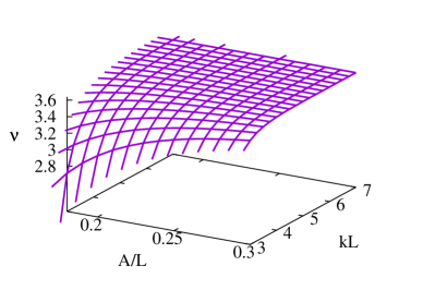
Figure 2: The dependence of turbulent viscosity $\nu_{A}(k)$ on the observation scale $\xi=A/L$ and the dimensionless momentum $x=kL$. Calculations were performed in the IR region using the equation (30) at the assumption of invariant $g_{A}\nu_{A}^{3}=g_{L}\nu_{L}^{3}$, i.e., small $K(\xi)$, and normalization momentum $x_{*}=4\pi$ used to evaluate $g_{L}$, in accordance to $k=2$ energy injection limit in simulated turbulence from John Hopkins Turbulence Database

The renormalized viscosity $\nu_{\xi}(k)$ is a counterpart of renormalized viscosity in the action of ordinary theory (5). The difference is that $\nu_{\xi}(k)$ is taken not in IR-stable fixed point, and therefore describes the asymptotic behavior of large-scale eddies, but is taken at a fixed observation scale $A=\xi L$. In terms of the scale-dependent action $S[u_{a},u_{a}^{\prime}]$ $\nu_{\xi}(k)$ can be understood as a viscosity acting on the wavelet-type pulsations of the velocity field $u_{a}(x)$ measured at scale $A$. The wave vector $k$ of such perturbations can take arbitrary values.

In this paper we neither aim to construct a turbulent stress tensor, as is presented in statistical filtering theory Eyink (1996) for the wave vectors less or equal to $1/a$, nor we construct statistical closures for scale-dependent fields $\mathbf{u}_{a}(x)$ for it would result in integral equations. Instead, since what is really measured in turbulence are the $n$-point correlation functions, we consider the Fourier transform of such functions $\langle\tilde{\mathbf{u}}_{a_{1}}(k_{1})\ldots\tilde{\mathbf{u}}_{a_{n}}(k_{n})\rangle$, where the wave vectors $k_{i}$ are responsible for the separation between the observation points, while the scale arguments $a_{i}$ are responsible for the observation scales.

V Energy spectra

The full kinetic energy of homogeneous isotropic turbulence can be expressed in terms of scale components of the velocity field: $E=\frac{1}{2}\int\langle|{\tilde{\mathbf{u}}}_{a}(\mathbf{k})|^{2}\rangle\frac{d^{d}k}{(2\pi)^{d}}\frac{1}{C_{g}}\frac{da}{a}$.

Figure 3: Feynman diagrams used for evaluation of the pair correlator of velocity field

We evaluate the the equal-time pair correlator $C(k,\xi)=\langle\tilde{u}_{A}(t,\mathbf{k})\tilde{u}_{A}(t,-\mathbf{k})\rangle$ of velocity field wavelet coefficients according the diagram rule shown in Fig. 3. The first term, the bare correlator integrated over the frequency and two internal scales, is equal to

$$C^{(0)}=\frac{1}{\nu_{0}k^{2}}\frac{g_{0}\nu_{0}^{3}}{L}(Lk)^{2}e^{-(Lk)^{2}}|\tilde{g}(Ak)|^{2}P_{ik}(\mathbf{k}).$$ (31)

The next contribution comes from the symmetric diagram in first line of Fig. 3, integrated over the frequency arguments. This gives

$$C^{(2)}=\frac{1}{2}\left(\frac{g_{0}\nu_{0}^{3}}{2C_{g}}\right)^{2}\frac{L^{2}k^{3}}{16\nu_{0}^{3}}|\tilde{g}(Ak)|^{2}f^{2}(Ak)P_{ik}(\mathbf{k})\int\frac{y^{2}dy}{(2\pi)^{2}}\frac{e^{-2(Lk)^{2}(1+2\xi^{2})\left(\frac{1}{4}+y^{2}\right)}\left(\frac{1}{4}+y^{2}\right)}{4\left(\frac{1}{4}+y^{2}\right)\nu_{0}k^{2}\left(1+\frac{1}{2}\left(\frac{1}{4}+y^{2}\right)\right)}\int d\mu\frac{(1-\mu^{2})(8\mu^{2}y^{2}+4y^{2}+1)}{\left(\frac{1}{4}+y^{2}-y\mu\right)\left(\frac{1}{4}+y^{2}+y\mu\right)},$$ (32)

where $f(Ak)=e^{-(Ak)^{2}}$ are wavelet filters in the legs of diagram. $1/2$ before the whole equation is a topological factor.

Two last diagrams in Fig. 3 contribute equally to the correlation function. Their joint contribution is

$$2C^{(1)} = -2P_{ik}(\mathbf{k})|\tilde{g}(Ak)|^{2}f^{2}(Ak)\frac{g_{0}\nu_{0}^{3}}{C_{g}L}|\tilde{g}(Lk)|^{2}\frac{g_{0}kL}{128C_{g}}\int\frac{y^{4}dy}{(2\pi)^{2}}\frac{e^{-(Lk)^{2}(1+4\xi^{2})\left(\frac{1}{4}+y^{2}\right)}}{2(\nu_{0}k^{2})^{2}\left(1+2\left(\frac{1}{4}+y^{2}\right)\right)}\times$$

$$\times \int d\mu\frac{(1-\mu^{2})(8\mu^{2}y^{2}+2\mu y(4y^{2}-5)+4y^{2}+1)}{\left(\frac{1}{4}+y^{2}-y\mu\right)\left(\frac{1}{4}+y^{2}+y\mu\right)}e^{-(kL)^{2}y\mu}.$$ (33)

The common sign minus stands for the fact $\Sigma^{\delta}$ is equal to minus diagram.

The final equation, without common wavelet factor $\tilde{g}(kA)\bar{\tilde{g}}(kA)$ on the legs of each diagram, calculated with $g_{1}$ wavelet is given by:

$$C(k,\xi)=\frac{g_{0}\nu_{0}^{3}}{\nu_{A}(k)}Le^{-(Lk)^{2}}$$

$$+ \frac{(g_{0}\nu_{0}^{3})^{2}}{128}\frac{(Lk)L}{\nu_{A}^{4}(k)}e^{-2\xi^{2}(Lk)^{2}}\int_{0}^{\infty}\frac{y^{2}dy}{(2\pi)^{2}}\frac{e^{-2(kL)^{2}(1+2\xi^{2})\left(\frac{1}{4}+y^{2}\right)}}{1+\frac{1}{2}\left(\frac{1}{4}+y^{2}\right)}\int_{-1}^{1}d\mu\frac{(1-\mu^{2})(8\mu^{2}y^{2}+4y^{2}+1)}{\left(\frac{1}{4}+y^{2}-y\mu\right)\left(\frac{1}{4}+y^{2}+y\mu\right)}+\frac{(g_{0}\nu_{0}^{3})^{2}}{32}\frac{(Lk)L}{\nu_{A}^{4}(k)}$$

$$\times e^{-(Lk)^{2}(1+2\xi^{2})}\int_{0}^{\infty}\frac{y^{4}dy}{(2\pi)^{2}}\frac{e^{-(kL)^{2}(1+4\xi^{2})\left(\frac{1}{4}+y^{2}\right)}}{1+2\left(\frac{1}{4}+y^{2}\right)}\int_{-1}^{1}d\mu\frac{(\mu^{2}-1)(8\mu^{2}y^{2}+2\mu y(4y^{2}-5)+4y^{2}+1)}{\left(\frac{1}{4}+y^{2}-y\mu\right)\left(\frac{1}{4}+y^{2}+y\mu\right)}e^{-(kL)^{2}y\mu}.$$ (34)

The coupling $g_{0}$ is related to the mean energy dissipation rate per unit of mass $\varepsilon$ by the energy balance equation $\varepsilon L^{4}=g_{0}\nu_{0}^{3}\chi[g],$ where $\chi[g]$ is numeric factor, which depends on the shape of basic wavelet (21). For the $g_{1}$ wavelet used in this paper $\chi[g_{1}]=\frac{3}{8\pi^{3/2}}$.

The obtained function (34) can be used to study the dependence of the turbulent pulsations energy spectrum $E(x,\xi)=4\pi k^{2}C(k,\xi)$, which is assumed to be Kolmogorov spectrum, if there is no dependence on the observation scale $\xi=A/L$.

We have compared our results with the $1024^{3}$ grid simulations of homogeneous isotropic turbulence presented in John Hopkins Turbulence Database (JHTDB) and described, e.g., in Li et al. (2008), with the following parameters of simulation: cubic domain of size $L=2\pi$, Kolmogorov length $l=0.0028$, dissipation rate $\varepsilon=0.103$, viscosity $\nu_{0}=0.000185$.

In traditional theory of turbulence the dependence of results of measurements, viz. the fields $v_{\delta}:=\frac{1}{\delta^{d}}\int v(x)d^{d}x$ and their statistical momenta, on the averaging scale $\delta$ is usually considered as an artifact of inappropriate choice: if $\delta$ is too small, say is close to the mean free path, we may get out of applicability of hydrodynamic approximation; alternatively, if it is too large, that is of the same order as the system size $L$, we get out of the limits of the Kolmogorov theory. Thus the ”legitimate” choice of observation scale lies deeply inside the Kolmogorov range of scales: $l\ll\delta\ll L$. Experimental processing of turbulence data stepped a little further when the wavelet transform was used to study turbulence behavior in ($k,a$) plane Vergassola and Frisch (1991). The study of distributions in ($k,a$) plane gives more information than that in $k$ only: the window width ($a$) for each mode ($k$) may tell whether this mode originates from the small or from the large scale dynamics.

In the limit of large observation scales $a\lesssim L$ there is no need for pulsations $u_{a}(k)$ to obey Kolmogorov’s laws. The energy of such pulsations decreases with the increase of resolution $a\to L$. The analytic tools, based on continuous wavelet transform, we propose in this paper may be useful in analytical computations of correlations of velocity pulsations measured at different spatial resolution.

As we can see from Fig. 4, the slope of the curves $E(k,\xi)$ depends on the observation scale $\xi$. The curves $A=0.1,0.2$, corresponding to small observation scales, i.e. those more than an order of magnitude less than external scale $L$, have the slopes close to the Kolmogorov $k^{-\frac{5}{3}}$ regime. In contrast, the larger observation window $A=0.5,1.0$, i.e. only one order less than $L$, results in a steeper falloff of the energy curves. Same thing happens with the dependence of energy on the dimensionless wave vector $x=kL$. Our analyzing wavelet $\tilde{g}(ak)\sim(ak)e^{-\frac{(ak)^{2}}{2}}$ is mostly sensitive to the wave numbers $k\sim\frac{1}{a}$, hence the observation scale $A\sim 0.1$ results in dimensionless wavevectors of the order $x\sim\frac{2\pi}{0.1}\approx 63$, and similar for other curves, which qualitatively agrees with that observed in Fig. 4.

The spectral index is close to the Kolmogorov value $-\frac{5}{3}$ for the values of observation scale in the middle of the inertial range $\xi_{0}\ll\xi\ll 1,$ but becomes steeper when approaching the dissipation scale $\xi_{0}$. Since our correlation functions (34) represent only partial energies of the given scale $\xi=A/L$ fluctuations, only the slopes can be compared. The integral over all scales should give a ”no-scale” energy spectrum. Since we are interested in the dependence of the energy spectra on the observation scale $\xi$ in Fig. 4 we present the graphs of such spectra and the standard ”no-scale” spectrum (shown in dashed line) obtained from numerical simulations http://turbulence.pha.jhu.edu

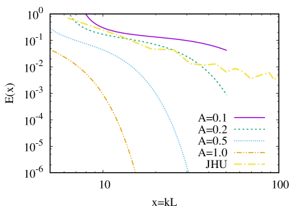
Figure 4: One dimensional energy spectra. Calculated for the set of parameters of the John Hopkins Turbulence Database for the isotropic turbulence grid simulations. The curves show the spectra for observation scales $A=0.1,0.2,0.5,1.0$. The $E(k)$ numerical energy spectrum, obtained for the $128^{3}$ decimation of the original JHTDB $1024^{3}$ data, is shown by dashed line. The normalization scale $x_{*}=4\pi$ corresponds to the $k=2$ energy injection limit. All quantities are normalized to $(2\pi)^{3}$ volume

VI Conclusion

We conclude, that using the multiscale representation of fields in field-theoretic calculations of turbulent velocity correlations we can obtain more information on the statistics of turbulent pulsations, than by standard spectral methods. Presented formalism is more relevant to experimental studies: any measured statistics of turbulent pulsations is always obtained at certain observation scale by averaging velocity fluctuations over the measuring volume. This volume should be somehow taken into account by theoretical description of turbulence.

It should be noted that our method of renormalization, acting from larger scales to smaller scales, ignores any effects of inverse energy cascade. This is significant simplification. The authors think, however, that a rigorous approach to the effect of small scale fluctuations on large scale fluctuations, which remains a chalenging problem, would involve more complicated description than just the forced Navier-Stokes equation itself. First of all the parity breaking effects and the inviscid topological invariants should be taken into account Chkhetiani et al. (2006b). The complexity of the problem can be seen for instance from the recent paper McComb and Yoffe (2017). We can hardly foresee such theory of an incompressible fluid flow capable of analytic calculations in the nearest future. The incompressibility itself is also a simplification. Wavelets might be of some use here as well, but up to the best authors knowledge their use in studying inverse energy cascade is limited to numerical simulation Meneveau (1991b).

From experimental point of view the dependence of the energy spectra on the observation scale $A$ becomes important when that scale approaches the Kolmogorov dissipative length $l$. In this limit the really observed steepness of the energy spectra should significantly exceed the Kolmogorov value of $-5/3$. In the opposite case, if the observation scale $A$ approaches the system size $L$, the steepness also increases for a large scale aperture can hardly resolve the energy-containing range fluctuations. If the observation scale belongs to the inertial range, the steepness is utmost equal to the Kolmogorov value, and does not significantly depend on scale Adzhemyan et al. (1998).

Appendix A Large scale stirring force

According to the Kolmogorov hypotheses, the energy injection should be equal to viscous energy dissipation per unit of mass. For stationary turbulence, to justify that the rate of energy dissipation per unit of mass

$$\varepsilon=\frac{d}{dt}\frac{\langle\mathbf{u}^{2}(t,\mathbf{x})\rangle}{2}=\langle\dot{u}_{i}(t,\mathbf{x})u_{i}(t,\mathbf{x})\rangle$$ (35)

is compensated by the stirring force $f$, we chose the random force correlator by defining the correlation function of its scale components:

$$\langle\tilde{f}_{ai}(t,\mathbf{k})\tilde{f}_{a^{\prime}j}(t^{\prime},\mathbf{k}^{\prime})\rangle=\delta(t-t^{\prime})P_{ij}(\mathbf{k})g_{0}\nu_{0}^{3}C_{g}(2\pi)^{d}\delta^{d}(\mathbf{k}+\mathbf{k}^{\prime})a\delta(a-a^{\prime})\delta(a-L),$$

where $g_{0}$ is formal dimensionless strength of forcing, to be used for the perturbation expansion (Adzhemyan et al., 1996). The delta-functions in scale arguments ensure that fluctuations of different scales $a$ and $a^{\prime}$ are uncorrelated, and the work is exerted over the fluid only at large scale $a=L$.

Reconstruction of Eulerian velocities $u_{i}$ from their scale components $u_{ai}$ by means of inverse wavelet transform gives

$$\langle\dot{u}_{i}(t,\mathbf{x})u_{i}(t,\mathbf{x})\rangle = \frac{1}{C_{g}^{2}}\int\exp(\imath\mathbf{x}(\mathbf{k}_{1}+\mathbf{k}_{2}))\tilde{g}(a_{1}\mathbf{k}_{1})\tilde{g}(a_{2}\mathbf{k}_{2})\langle\tilde{f}_{a_{1}i}(t,\mathbf{k}_{1})\int^{t}\tilde{f}_{a_{2}i}(\tau,\mathbf{k}_{2})d\tau\rangle\frac{d^{d}\mathbf{k}_{1}}{(2\pi)^{d}}\frac{da_{1}}{a_{1}}\frac{d^{d}\mathbf{k}_{2}}{(2\pi)^{d}}\frac{da_{2}}{a_{2}}$$

$$= \frac{g_{0}\nu_{0}^{3}}{L^{d+1}}\frac{(d-1)}{2C_{g}}\int_{0}^{\infty}|\tilde{g}(\mathbf{y})|^{2}\frac{d^{d}\mathbf{y}}{(2\pi)^{d}},$$ (36)

where factor $(d-1)$ comes from the trace of orthogonal projector, and the factor $\frac{1}{2}$ is the value of the $\theta$-function at the discontinuity. For particular case of

$$\tilde{g}_{1}(k)=-\imath\mathbf{k}e^{-\mathbf{k}^{2}/2}$$

wavelet in $d=3$ dimensions, we get

$$\quad C_{g}=\frac{1}{2},\quad\int_{0}^{\infty}y^{2}e^{-y^{2}}\frac{4\pi y^{2}dy}{8\pi^{3}}=\frac{3}{16\pi^{3/2}}\equiv\frac{\chi[g_{1}]}{2},$$

Substituting this integral into (36) one gets

$$\varepsilon=\frac{g_{0}\nu_{0}^{3}}{L^{4}}\frac{3}{8\pi^{3/2}}.$$ (37)

Appendix B Feynman diagram technique

Using the generating functional (19) with the action (20) we can easily derive the Feynman diagram technique for the scale-dependent fields $\Phi_{a}$.

The correlation functions are given by functional derivatives

$$\langle\Phi_{a_{1}}(x_{1})\ldots\Phi_{a_{n}}(x_{n})\rangle_{c}=\left.\frac{\delta^{n}W[A]}{\delta A_{a_{1}}(x_{1})\ldots\delta A_{a_{n}}(x_{n})}\right|_{A=0}.$$

The difference is that each spatial integration measure $dx$ is substituted by the integration measure over affine group $\frac{dxda}{a}$, with functional derivatives taken with respect to this measure.

Using the Fourier transform

$$u(x)=\int e^{\imath(\mathbf{k}\mathbf{x}-\omega t)}u(k)\frac{d^{d}\mathbf{k}d\omega}{(2\pi)^{d+1}}$$

of the fields in (20) we make each convolution with basic wavelet $g$ into a multiplicative factor $\tilde{g}(a\mathbf{k})$. In this way we obtain the following diagram technique:

• Each external line is labeled by a pair $(a,k)$ (scale,momentum), and a vector index ($i$).

• The integration in each internal line is performed over the measure $\frac{d\omega}{2\pi}\frac{d^{d}\mathbf{k}}{(2\pi)^{d}}\frac{da}{a}\frac{1}{C_{g}}$.

• There are two type of lines: a) Green functions $\langle uu^{\prime}\rangle$ and b) correlation functions $\langle uu\rangle$; The auxiliary field $u^{\prime}$ has zero moments $\langle u^{\prime}u^{\prime}\rangle=0$. These Green functions are given by propagator matrix $K^{-1}$ multiplied by wavelet factors $\tilde{g}(a\mathbf{k})$ on each leg.

• Each line carrying momentum $k$ is proportional to orthogonal projector $P_{ij}(\mathbf{k})$, where $i$ and $j$ are vector indices of the line, i.e.

  $$G^{(0)}_{i\alpha,j\beta}(k)=\frac{\tilde{g}(\alpha\mathbf{k})P_{ij}(\mathbf{k})\overline{\tilde{g}}(\beta\mathbf{k})}{-\imath\omega+\nu_{0}\mathbf{k}^{2}}$$

  for the Green function, and

  $$D^{(0)}_{i\alpha,j\beta}(k)=P_{ij}(\mathbf{k})\frac{g_{0}\nu_{0}^{3}}{C_{g}L}\frac{\tilde{g}(\alpha\mathbf{k})|\tilde{g}(kL)|^{2}\bar{\tilde{g}}(\beta\mathbf{k})}{|-\imath\omega+\nu_{0}\mathbf{k}^{2}|^{2}}$$

  for the bare velocity pair correlation function.

• Each vertex of the diagram is given by $m_{abc}(k)=\frac{\imath}{2}\left(k_{b}\delta_{ac}+k_{c}\delta_{ab}\right),$ multiplied by 3 wavelet factors of adjusted lines.

• We consider the observation scale $A$ to be much bigger than the viscous dissipation scale $l$ and to belong the Kolmogorov range: $\xi=A/L\ll 1$. For this reason we assume the statistical momenta of the turbulent velocity field are determined by direct energy cascade. At the language of Feynman diagrams this means it should be no scales $a_{i}$ in internal lines less than minimal scale of all external lines.

Appendix C One-loop contributions to the Green functions

The scale dependence of the viscosity is given by renormalization of the Green function $\langle\Phi_{\alpha}(x)\Phi_{\beta}(x^{\prime})\rangle$ by means of loop corrections. In Fourier space the value of the Green function $G^{(2)}_{\alpha a,\beta s}(k)$, shown in diagram Fig. 1, can be evaluated from the above mentioned expressions for the vertices and the Green functions after the integration over internal line scale arguments. The upper line of the diagram Fig. 1, ($p^{+}$), contains the random stirring force correlator, the bottom line ($p^{-}$) is the Green function.

The frequency integration in the loop integral can be done explicitly

$$\int_{-\infty}^{\infty}\frac{dq_{0}}{2\pi}|G_{0}(\frac{k}{2}+q)|^{2}G_{0}(\frac{k}{2}-q) = \frac{1}{2\nu_{0}^{2}(\frac{\mathbf{k}}{2}+\mathbf{q})^{2}}\times$$

$$\times \frac{1}{-\frac{\imath k_{0}}{\nu_{0}^{2}}+\frac{\mathbf{k}^{2}}{2}+2\mathbf{q}^{2}}$$

where

$$G_{0}(k)=\frac{1}{-\imath k_{0}+\nu_{0}\mathbf{k}^{2}}.$$

The loop tensor structure $L_{as}(k,p^{+},p^{-})$ (24) is given by the convolution of

$$L(k,p^{+},p^{-})=m_{abc}(k)m_{fls}(p^{-})P_{bl}(p^{+})P_{cf}(p^{-}),$$ (38)

where

$$m_{abc}(k)=\frac{\imath}{2}\left(k_{b}\delta_{ac}+k_{c}\delta_{ab}\right),\quad p^{\pm}=\frac{k}{2}\pm q,$$

over repeated indices. The explicit equation for tensor structure is equation (24).

Let $A=\min(\alpha,\beta)$ be the minimal scale of two external lines of the diagram Fig. 1. The lower line ($p^{-}$) contributes two identical $g_{1}$ wavelet factors

$$e^{-(A\mathbf{p}^{-})^{2}}=\frac{1}{C_{g}}\int_{A}^{\infty}|\tilde{g}(a\mathbf{p}^{-})|^{2}\frac{da}{a},$$

so, the factor $e^{-2(A\mathbf{p}^{-})^{2}}$ will be prescribed to the bottom line; and similar factor $e^{-2(A\mathbf{p}^{+})^{2}}$ to the upper line.

Introducing the dimensionless momentum $\mathbf{q}=|\mathbf{k}|\mathbf{y}$, with the polar angle between $\mathbf{q}$ and $\mathbf{k}$ measured from the $\mathbf{k}$ direction, we can write the whole one-loop integral in $d=3$ dimension in the form

$$-\Sigma_{as}(k) = \frac{g_{0}\nu_{0}^{3}}{C_{g}L}\int k^{3}\frac{y^{2}dy}{(2\pi)^{3}}\sin\theta d\theta d\varphi L_{as}(k,p^{+},p^{-})\frac{1}{\nu_{0}^{2}k^{4}}\frac{1}{\frac{1}{2}+2y^{2}+2y\cos\theta}\frac{1}{\frac{1}{2}+2y^{2}-\frac{\imath k_{0}}{\nu_{0}k^{2}}}\times$$

$$\times (Lk)^{2}\left[\frac{1}{4}+y^{2}+y\cos\theta\right]e^{-(Lk)^{2}\left[\frac{1}{4}+y^{2}+y\cos\theta\right]}e^{-2(Lk)^{2}\xi^{2}\left[\frac{1}{4}+y^{2}-y\cos\theta\right]}e^{-2(Lk)^{2}\xi^{2}\left[\frac{1}{4}+y^{2}+y\cos\theta\right]}.$$

This can be simplified to

$$-\Sigma_{as}(k)=\frac{g_{0}\nu_{0}^{3}C_{g}^{-1}Lk}{4\nu_{0}^{2}}\int\frac{y^{2}dy}{(2\pi)^{3}}\sin\theta d\theta d\varphi L_{as}(k,p_{+},p_{-})\frac{1}{\frac{1}{4}+y^{2}-\frac{\imath k_{0}}{2\nu k^{2}}}$$

The sign $-\Sigma$ is introduced for the value of one-loop integral is equal to minus ”self-energy” contribution.

In view of the existence of only one preferred direction, that is the direction of $\mathbf{k}$, the integrals of $L_{as}$ should depend upon two scalars only:

$$T_{1}\equiv{\rm Tr}L_{as},\quad T_{2}=\frac{k_{a}k_{s}}{k^{2}}L_{as}$$ (39)

$$T_{1} = -\frac{(p^{-}k)(p^{+}p^{-})^{2}}{2(p^{+})^{2}(p^{-})^{2}}+\frac{(p^{+}k)(p^{+}p^{-})}{(p^{+})^{2}}-\frac{(p^{-}k)}{2},$$

$$T_{2} = -\frac{(p^{+}k)(p^{+}p^{-})(p^{-}k)^{2}}{(p^{+})^{2}(p^{-})^{2}k^{2}}+\frac{(p^{-}k)(p^{+}k)^{2}}{2(p^{+})^{2}k^{2}}$$

$$+ \frac{(p^{+}k)(p^{+}p^{-})k^{2}}{2(p^{+})^{2}k^{2}}+\frac{(p^{-}k)^{3}}{(p^{-})^{2}k^{2}}-(p^{-}k).$$

Assuming

$$\Sigma_{as}=\nu_{0}g_{0}\Sigma^{\delta}\delta_{as}k^{2}+\nu_{0}g_{0}\Sigma^{T}k_{a}k_{s}=-\int L_{as}d\mu(y,\theta),$$ (40)

we get

$$(d\Sigma^{\delta}+\Sigma^{T})k^{2} = -\int T_{1}d\mu(y,\theta)=-k^{2}I_{1},$$

$$(\Sigma^{\delta}+\Sigma^{T})k^{2} = -\int T_{2}d\mu(y,\theta)=-k^{2}I_{2},$$

where $d\!=\!3$ is the space dimension. So, we need to calculate $I_{1}$ and $I_{2}$. From where

$$\Sigma^{\delta}=-\frac{I_{1}-I_{2}}{2},\quad\Sigma^{T}=-I_{2}-\Sigma^{\delta}=-\frac{3I_{2}-I_{1}}{2}.$$

The substitution $\mathbf{q}=k\mathbf{y},(kq)=ky\mu$, with $\mu\equiv\cos\theta$, gives:

$$T_{1} = {\rm Tr}L_{as}=k^{2}\frac{-\mu^{3}y^{3}+2\mu^{2}y^{4}+\mu y^{3}-2y^{4}}{2\left[\left(\frac{1}{4}+y^{2}\right)^{2}-y^{2}\mu^{2}\right]}=\frac{8k^{2}(\mu-1)(\mu+1)(2y-\mu)y^{3}}{(4y^{2}-4y\mu+1)(4y^{2}+4y\mu+1)},$$

$$T_{2} = \frac{k_{a}k_{s}}{k^{2}}L_{as}=k^{2}\frac{-\mu^{3}y^{5}+\mu y^{5}-\mu^{4}y^{4}+\frac{5}{2}\mu^{2}y^{4}-\frac{3}{2}y^{4}+\frac{1}{4}\mu^{3}y^{3}-\frac{1}{4}\mu y^{3}-\frac{1}{8}\mu^{2}y^{2}+\frac{1}{8}y^{2}}{2(1/4+y\mu+y^{2})(1/4-y\mu+y^{2})}$$

$$= -k^{2}\frac{(\mu-1)(\mu+1)(8\mu y^{3}+8\mu^{2}y^{2}-12y^{2}-2\mu y+1)}{(4y^{2}-4y\mu+1)(4y^{2}+4y\mu+1)}y^{2},$$

$$\frac{T_{1}-T_{2}}{2} = k^{2}\frac{(\mu^{2}-1)y^{2}(8\mu^{2}y^{2}+\mu(8y^{3}-10y)+4y^{2}+1)}{2(4y^{2}-4y\mu+1)(4y^{2}+4y\mu+1)},$$

$$\frac{3T_{2}-T_{1}}{2} = -k^{2}\frac{(\mu^{2}-1)y^{2}(24\mu^{2}y^{2}+\mu(24y^{3}-14y)-20y^{2}+3)}{2(4y^{2}-4y\mu+1)(4y^{2}+4y\mu+1)}.$$

After standard algebraic manipulations, this gives:

$$\Sigma^{\delta} = \frac{kL}{128C_{g}}\int_{0}^{\infty}\frac{y^{2}dy}{(2\pi)^{2}}\frac{e^{-(kL)^{2}(1+4\xi^{2})\left(\frac{1}{4}+y^{2}\right)}}{\frac{1}{4}+y^{2}-\imath\frac{2k_{0}}{\nu_{0}\mathbf{k}^{2}}}\int_{-1}^{1}d\mu\frac{(1-\mu^{2})(8\mu^{2}y^{2}+\mu(8y^{3}-10y)+4y^{2}+1)}{\left(\frac{1}{4y}+y-\mu\right)\left(\frac{1}{4y}+y+\mu\right)}e^{-(kL)^{2}y\mu},$$ (41)

$$\Sigma^{T} = -\frac{kL}{128C_{g}}\int_{0}^{\infty}\frac{y^{2}dy}{(2\pi)^{2}}\frac{e^{-(kL)^{2}(1+4\xi^{2})\left(\frac{1}{4}+y^{2}\right)}}{\frac{1}{4}+y^{2}-\imath\frac{2k_{0}}{\nu_{0}\mathbf{k}^{2}}}\int_{-1}^{1}d\mu\frac{(1-\mu^{2})(24\mu^{2}y^{2}+\mu(24y^{3}-14y)-20y^{2}+3)}{\left(\frac{1}{4y}+y-\mu\right)\left(\frac{1}{4y}+y+\mu\right)}e^{-(kL)^{2}y\mu},$$

where $\mu=\cos\theta$ determines the polar angle between $\mathbf{k}$ and $\mathbf{q}$. Since the velocity field is transversal, it is natural to present the self-energy as a sum of transversal and longtitudal terms:

$$\Sigma_{as}=\nu g\Sigma^{\delta}\left(\delta_{as}-\frac{k_{a}k_{s}}{\mathbf{k}^{2}}\right)\mathbf{k}^{2}+\nu g\Sigma^{l}k_{a}k_{s},$$ (42)

where $\Sigma^{l}=\Sigma^{\delta}+\Sigma^{T}$.

Appendix D One-loop contribution to stirring force correlator

The one-loop contribution to stirring force correlator is shown in Fig. 5 below.

Figure 5: One-loop contribution to the correlation function. Greek letters $\alpha$ and $\beta$ denote scale arguments.

The tensor structure of this diagram has the form

$$C_{as}(k,p^{+},p^{-})=-m_{abc}(k)m_{sfl}(k)P^{bl}(\mathbf{p}^{+})P^{cf}(\mathbf{p}^{-}),$$ (43)

or explicitly:

$$C_{as}(k,p^{+},p^{-}) = \delta_{as}\left[k^{2}-\frac{(p^{+}k)^{2}}{4(p^{+})^{2}}-\frac{(p^{-}k)^{2}}{4(p^{-})^{2}}\right]+\frac{k_{a}k_{s}}{2}$$

$$+ \frac{p^{+}_{a}p^{+}_{s}}{4}\left[\frac{(p^{-}k)^{2}}{(p^{-})^{2}(p^{+})^{2}}-\frac{k^{2}}{(p^{+})^{2}}\right]$$

$$+ \frac{p^{-}_{a}p^{-}_{s}}{4}\left[\frac{(p^{+}k)^{2}}{(p^{-})^{2}(p^{+})^{2}}-\frac{k^{2}}{(p^{-})^{2}}\right]$$

$$= (p^{+}_{a}p^{-}_{s}+p^{-}_{a}p^{+}_{s})\frac{(p^{+}k)(p^{-}k)}{4(p^{+})^{2}(p^{-})^{2}}$$

$$- (k_{a}p^{+}_{s}+p^{+}_{a}k_{s})\frac{(p^{+}k)}{4(p^{+})^{2}}$$

$$- (k_{a}p^{-}s+p^{-}_{a}k_{s})\frac{(p^{-}k)}{4(p^{-})^{2}}.$$

The corresponding invariants, the tensor structure can depend on, are

$$C_{1} = {\rm Tr}C_{as} = \frac{3}{2}k^{2}-\frac{(p^{-}k)^{2}}{(p^{-})^{2}}-\frac{(p^{+}k)^{2}}{(p^{+})^{2}}$$

$$+ \frac{(p^{+}k)(p^{-}k)(p^{+}p^{-})}{2(p^{+})^{2}(p^{-})^{2}},$$

$$C_{2} = \frac{k^{a}k^{s}}{k^{2}}C_{as} = k^{2}-\frac{(p^{-}k)^{2}}{(p^{-})^{2}}-\frac{(p^{+}k)^{2}}{(p^{+})^{2}}$$

$$+ \frac{(p^{-}k)^{2}(p^{+}k)^{2}}{(p^{-})^{2}(p^{+})^{2}}.$$

In dimensionless variables

$$C_{1} = -\frac{2k^{2}(\mu^{2}-1)y^{2}(12y^{2}+1)}{(4y^{2}-4y\mu+1)(4y^{2}+4y\mu+1)},$$

$$C_{2} = \frac{16k^{2}(\mu^{2}-1)^{2}y^{4}}{(4y^{2}-4y\mu+1)(4y^{2}+4y\mu+1)},$$

$$\frac{C_{1}-C_{2}}{2} = -\frac{k^{2}(\mu^{2}-1)y^{2}(8y^{2}\mu^{2}+4y^{2}+1)}{(4y^{2}-4y\mu+1)(4y^{2}+4y\mu+1)},$$

$$\frac{3C_{2}-C_{1}}{2} = \frac{k^{2}(\mu^{2}-1)y^{2}(24y^{2}\mu^{2}-12y^{2}+1)}{(4y^{2}-4y\mu+1)(4y^{2}+4y\mu+1)}.$$ (44)

The total symmetric contribution to the 1PI correlation function has the form

$$\Delta^{(2)}_{as} = \left(\frac{g_{0}\nu_{0}^{3}}{LC_{g}}\right)^{2}\int\frac{d^{4}q}{(2\pi)^{4}}\frac{|\tilde{g}(Lp^{+})|^{2}f^{2}(Ap^{+})}{|-\imath\omega^{+}+\nu_{0}(p^{+})^{2}|^{2}}$$

$$\times \frac{|\tilde{g}(Lp^{-})|^{2}f^{2}(Ap^{-})}{|-\imath\omega^{-}+\nu_{0}(p^{-})^{2}|^{2}}C_{as}(k,p^{+},p^{-}).$$

In case the non-zero frequency $k_{0}\neq 0$

$$\int_{-\infty}^{\infty}\frac{dq_{0}}{2\pi}\left|G_{0}\left(\frac{k}{2}+q\right)\right|^{2}\left|G_{0}\left(\frac{k}{2}-q\right)\right|^{2}=\frac{1}{4\nu_{0}^{3}}\frac{\frac{\mathbf{k}^{2}}{4}+\mathbf{q}^{2}}{\left(\frac{\mathbf{k}^{2}}{4}+\mathbf{q}^{2}+\imath\frac{2k_{0}}{\nu_{0}}\right)\left(\frac{\mathbf{k}^{2}}{4}+\mathbf{q}^{2}-\imath\frac{2k_{0}}{\nu_{0}}\right)}\cdot\frac{1}{\frac{\mathbf{k}^{2}}{4}+\mathbf{q}^{2}+\mathbf{k}\mathbf{q}}\cdot\frac{1}{\frac{\mathbf{k}^{2}}{4}+\mathbf{q}^{2}-\mathbf{k}\mathbf{q}}.$$ (45)

In case of the zero frequency $k_{0}=0$ this turns to be

$$\int_{-\infty}^{\infty}\frac{dq_{0}}{2\pi}\left|G_{0}\left(\frac{k}{2}+q\right)\right|^{2}\left|G_{0}\left(\frac{k}{2}-q\right)\right|^{2}=\frac{1}{4\nu_{0}^{3}}\frac{1}{\frac{\mathbf{k}^{2}}{4}+\mathbf{q}^{2}}\cdot\frac{1}{\frac{\mathbf{k}^{2}}{4}+\mathbf{q}^{2}+\mathbf{k}\mathbf{q}}\cdot\frac{1}{\frac{\mathbf{k}^{2}}{4}+\mathbf{q}^{2}-\mathbf{k}\mathbf{q}}.$$ (46)

The $\delta$-function in scale variables results in square of wavelets in both upper and lower parts of the loop

$$|\tilde{g}(Lp^{+})|^{2}|\tilde{g}(Lp^{-})|^{2} = L^{2}\left(\frac{\mathbf{k}}{2}+\mathbf{q}\right)^{2}e^{-L^{2}\left(\frac{\mathbf{k}}{2}+\mathbf{q}\right)^{2}}$$

$$\times L^{2}\left(\frac{\mathbf{k}}{2}-\mathbf{q}\right)^{2}e^{-L^{2}\left(\frac{\mathbf{k}}{2}-\mathbf{q}\right)^{2}}$$

The angle arguments in the exponents are canceled due to symmetry. The filter factors for $g_{1}$ wavelet are

$$f(Ap^{\pm})=e^{-(Ak)^{2}(1/4+y^{2}\pm y\cos\theta)}$$

After integration over the loop frequency variable $\int_{-\infty}^{\infty}\frac{dq_{0}}{2\pi}\ldots$ we get

$$\Delta^{(2)}_{as}=\left(\frac{g_{0}\nu_{0}^{3}}{LC_{g}}\right)^{2}(kL)^{4}\int\left[\left(\frac{1}{4}+y^{2}\right)^{2}-y^{2}\cos^{2}\theta\right]e^{-2(kL)^{2}\left(\frac{1}{4}+y^{2}\right)}\frac{1}{4\nu_{0}^{3}}\frac{\frac{\mathbf{k}^{2}}{4}+\mathbf{q}^{2}}{\left(\frac{\mathbf{k}^{2}}{4}+\mathbf{q}^{2}+\imath\frac{2k_{0}}{\nu_{0}}\right)\left(\frac{\mathbf{k}^{2}}{4}+\mathbf{q}^{2}-\imath\frac{2k_{0}}{\nu_{0}}\right)}\cdot$$

$$\frac{1}{\frac{\mathbf{k}^{2}}{4}+\mathbf{q}^{2}+\mathbf{k}\mathbf{q}}\cdot\frac{1}{\frac{\mathbf{k}^{2}}{4}+\mathbf{q}^{2}-\mathbf{k}\mathbf{q}}e^{-4\xi^{2}(Lk)^{2}\left(\frac{1}{4}+y^{2}\right)}C_{as}(k,p^{+},p^{-})\frac{q^{2}dq}{(2\pi)^{2}}\sin\theta d\theta.$$

After algebraic simplification we get

$$\Delta^{(2)}_{as}(L,k) = \left(\frac{g_{0}\nu_{0}^{3}}{2C_{g}}\right)^{2}\frac{L^{2}}{\nu_{0}^{3}}\int\frac{q^{2}dq}{(2\pi)^{2}}\sin\theta d\theta\frac{e^{-2(Lk)^{2}(1+2\xi^{2})\left(\frac{1}{4}+y^{2}\right)}C_{as}(k,p^{+},p^{-})\left(\frac{\mathbf{k}^{2}}{4}+\mathbf{q}^{2}\right)}{\left(\frac{\mathbf{k}^{2}}{4}+\mathbf{q}^{2}+\imath\frac{2k_{0}}{\nu_{0}}\right)\left(\frac{\mathbf{k}^{2}}{4}+\mathbf{q}^{2}-\imath\frac{2k_{0}}{\nu_{0}}\right)}.$$

In view of isotropy, using equation (44), we get

$$C_{as}=C^{\delta}\delta_{as}+C^{T}\frac{k_{a}k_{s}}{k^{2}}$$

with

$$C^{\delta}(L,k) = \left(\frac{g_{0}\nu_{0}^{3}}{2C_{g}}\right)^{2}\frac{L^{2}k^{3}}{16\nu_{0}^{3}}\int\frac{y^{4}dy}{(2\pi)^{2}}d\mu\frac{e^{-2(Lk)^{2}(1+2\xi^{2})\left(\frac{1}{4}+y^{2}\right)}\left(\frac{1}{4}+y^{2}\right)}{\left(\frac{1}{4}+y^{2}+\imath\frac{2k_{0}}{\nu_{0}\mathbf{k}^{2}}\right)\left(\frac{1}{4}+y^{2}-\imath\frac{2k_{0}}{\nu_{0}\mathbf{k}^{2}}\right)}\frac{(1-\mu^{2})(8y^{2}\mu^{2}+4y^{2}+1)}{\left(\frac{1}{4}+y^{2}-y\mu\right)\left(\frac{1}{4}+y^{2}+y\mu\right)}.$$ (47)

Appendix E Renormalization group equations

E.1 Renormalization of viscosity

We use the following set of scales $l=A_{0}<A_{1}<A_{2}<\ldots<A_{L}=L$. In terms of dimensionless variable $\xi=A/L$ this corresponds to $\xi_{0}=R^{-1},\xi_{1},\xi_{2},\ldots,\xi_{L}=1,$ where $R=L/l\gg 1$. If we use the iteration from the Kolmogorov dissipation scale $l$ to the macro scales, we would get the following chain of equations:

$$\nu_{1} = \nu_{0}[1+g_{0}\Sigma(\xi_{0})],$$

$$\nu_{2} = \nu_{1}[1+g_{1}\Sigma(\xi_{1})],$$

$$\nu_{k+1} = \nu_{k}[1+g_{k}\Sigma(\xi_{k})].$$

If we go from large scales to smaller scales the proposed inversion formulae are:

$$\nu_{0} \approx \nu_{1}[1-g_{1}\Sigma(\xi_{0})],$$

$$\nu_{1} \approx \nu_{2}[1-g_{2}\Sigma(\xi_{1})],$$

$$\nu_{k-1} \approx \nu_{k}[1-g_{k}\Sigma(\xi_{k-1})],$$ (48)

where $g_{k}\equiv g(\xi_{k})$. The iteration scheme above can be written in a form of difference equation

$$\frac{\nu_{k-1}-\nu_{k}}{\nu_{k}}=-g(\xi_{k})\Sigma(\xi_{k-1}).$$ (49)

For the equal scale steps $A_{k}=A_{0}\delta^{k},\xi_{k}=\xi_{0}\delta^{k},\Delta\ln\xi=\ln\delta\Delta k,$ we get

$$\frac{\Delta\ln\nu}{\Delta k}=g(\xi_{k})\Sigma(\xi_{k}),\quad\hbox{or\ }\frac{d\ln\nu}{d\ln\xi}=g(\xi)\frac{\Sigma(\xi)}{\ln\delta}.$$

E.2 Renormalization of stirring force

The one-loop contribution to the stirring force correlation function is shown in Fig. 5.

Since the stirring force acts on large scales only, its yield on smaller scales will be the sum of correlator itself and the one loop correction

$$D_{L-1}=D_{L}+D_{L}^{2}*OneLoopK(\xi_{L-1})$$ (50)

with $D(\xi)=g(\xi)\nu^{3}(\xi)/L$, hence

$$\frac{D_{L-1}-D_{L}}{D_{L}}=D_{L}*OneLoopK(\xi_{L-1}).$$

In differential form the latter difference equation yields

$$\frac{d\ln D}{d\ln\xi}=-\frac{K(\xi)}{\ln\delta}$$

where

$$K(\xi) = \frac{(kL)^{3}}{16}\int\frac{y^{4}dy}{(2\pi)^{2}}d\mu\frac{e^{-2(Lk)^{2}(1+2\xi^{2})\left(\frac{1}{4}+y^{2}\right)}\left(\frac{1}{4}+y^{2}\right)}{\left(\frac{1}{4}+y^{2}+\imath\frac{2k_{0}}{\nu_{0}\mathbf{k}^{2}}\right)\left(\frac{1}{4}+y^{2}-\imath\frac{2k_{0}}{\nu_{0}\mathbf{k}^{2}}\right)}\frac{(1-\mu^{2})(8y^{2}\mu^{2}+4y^{2}+1)}{\left(\frac{1}{4}+y^{2}-y\mu\right)\left(\frac{1}{4}+y^{2}+y\mu\right)}.$$ (51)

The value of $K(\xi)$ is typically a few orders of magnitude less than $\Sigma(\xi)$.

Appendix F Frequency integrals that contribute to velocity pair correlator

The bare correlation function, being integrated over the frequency, contains the integral

$$I_{w0}=\int_{-\infty}^{\infty}\frac{d\omega}{2\pi}\frac{1}{|-\imath\omega+A|^{2}}=\frac{1}{2A},\quad A=\nu\mathbf{k}^{2}$$ (52)

The integral coming from 1PI correlation function multiplied by two conjugated correlation functions from the legs of the diagram has the form

$$I_{w2}=\int_{-\infty}^{\infty}\frac{d\omega}{2\pi}\frac{1}{|-\imath\omega+A|^{2}}\frac{1}{|B+\imath\frac{2\omega}{A}|^{2}},\quad B=\frac{1}{4}+y^{2}.$$ (53)

Substituting $C=\frac{AB}{2}$, we get

$$I_{w2} = \int_{-\infty}^{\infty}\frac{d\omega}{2\pi}\frac{A^{2}}{4}\frac{1}{\omega^{2}+A^{2}}\frac{1}{\omega^{2}+C^{2}}=\frac{1}{8}\frac{A}{C(A+C)}$$

$$= \frac{1}{4\left(\frac{1}{4}+y^{2}\right)\nu\mathbf{k}^{2}\left(1+\frac{1}{2}\left(\frac{1}{4}+y^{2}\right)\right)}.$$

The third integral comes from two conjugated diagrams with self-energy multiplied by correlator and propagator

$$I_{1w} = \int_{-\infty}^{\infty}\frac{d\omega}{2\pi}\frac{1}{\omega^{2}+A^{2}}\cdot\frac{1}{-\imath\omega+A}\cdot\frac{2A}{4C-\imath\omega}$$

$$= \frac{1}{2A(A+4C)}=\frac{1}{2(\nu\mathbf{k}^{2})^{2}\left(1+2\left(\frac{1}{4}+y^{2}\right)\right)}.$$

This integral contributes twice for there are two conjugated diagrams, shown in the lower part of Fig. 3.

References

- Reynolds (1895) O. Reynolds, Phil. Trans. R. Soc. Lond. A 186, 123 (1895).
- Monin and Yaglom (1975) A. Monin and A. Yaglom, Statistical fluid mechanics, Vol. 2 (MIT Press, Cambridge, MA, 1975).
- McComb (1992) W. McComb, The Physics of Fluid Turbulence (Clarendon Press, 1992).
- Frisch (1995) U. Frisch, Turbulence: The legacy of A.N.Kolmogorov (Cambridge University Press, England, 1995).
- Kolmogorov (1941a) A. Kolmogorov, Dokl. Akad. Nauk SSSR 30, 9 (1941a), reprinted in Proc. R. Soc. Lond. A434, 9–13,1991.
- Kolmogorov (1941b) A. Kolmogorov, Dokl. Akad. Nauk SSSR 31, 538 (1941b).
- Kolmogorov (1962) A. Kolmogorov, J. Fluid. Mech. 13, 82 (1962).
- Obukhov (1962) A. Obukhov, J. Fluid. Mech. 13, 77 (1962).
- Huang et al. (2010) Y. X. Huang, F. G. Schmitt, Z. M. Lu, P. Fougairolles, Y. Gagne, and Y. L. Liu, Phys. Rev. E 82, 026319 (2010).
- Meneveau and Sreenivasan (1987) C. Meneveau and K. Sreenivasan, Phys. Rev. Lett. 59, 1424 (1987).
- Farge (1992) M. Farge, Annual review of fluid mechanics 24, 395 (1992).
- Yoshimatsu et al. (2009) K. Yoshimatsu, N. Okamoto, K. Schneider, Y. Kaneda, and M. Farge, Phys. Rev. E 79, 026303 (2009).
- Wilson and Kogut (1974) K. G. Wilson and J. Kogut, Phys. Rep. 12, 75 (1974).
- Vasil’ev (2004) A. Vasil’ev, The field theoretic renormalization group in critical behavior theory and stochastic dynamics (Chapman & Hall/CRC, 2004).
- Forster et al. (1977) D. Forster, D. Nelson, and M. Stephen, Phys. Rev. A 16, 732 (1977).
- Adzhemyan et al. (1983) L. Adzhemyan, A. Vasil’ev, and Y. M. Pis’mak, Theoretical and Mathematical Physics 57, 1131 (1983).
- Yakhot and Orszag (1986a) V. Yakhot and S. Orszag, Phys. Rev. Lett. 57, 1722 (1986a).
- Yakhot and Orszag (1986b) V. Yakhot and S. Orszag, J. Sci. Comp 1, 1 (1986b).
- Adzhemyan et al. (1996) L. T. Adzhemyan, N. V. Antonov, and A. N. Vasil’ev, Physics-Uspekhi 39, 1193 (1996).
- Martin et al. (1973) P. Martin, E. Sigia, and H. Rose, Phys. Rev. A8, 423 (1973).
- Altaisky et al. (1990) M. Altaisky, S. Moiseev, and S. Pavlik, Phys. Lett. A 147, 142 (1990).
- Kolmogorov (1941c) A. Kolmogorov, Dokl. Akad. Nauk SSSR 32, 16 (1941c), reprinted in Proc. R. Soc. Lond. A434,15–17,1991.
- Hnatič et al. (2018) M. Hnatič, G. Kalagov, and M. Nalimov, Nucl. Phys. B 926, 1 (2018).
- Eyink (1996) G. Eyink, J. Stat. Phys. 83, 955 (1996).
- Collins (1984) J. C. Collins, Renormalization (Cambridge University Press, England, 1984).
- Antonov et al. (2003) N. Antonov, M. Hnatich, J. Honkonen, and M. Jurčišin, Phys. Rev. E 68, 046306 (2003).
- Altaisky (2010) M. V. Altaisky, Phys. Rev. D 81, 125003 (2010).
- Altaisky and Kaputkina (2013) M. V. Altaisky and N. E. Kaputkina, Phys. Rev. D 88, 025015 (2013).
- Zimin (1981) V. Zimin, Izv. Atmos. Ocean. Phys. 17, 941 (1981).
- Meneveau (1991a) C. Meneveau, J. Fluid. Mech. 232, 469 (1991a).
- Yamada and Ohkitani (1991) M. Yamada and K. Ohkitani, Fluid Dynamics Research 8, 101 (1991).
- Vergassola and Frisch (1991) M. Vergassola and U. Frisch, Physica D 54, 58 (1991).
- Astafieva (1996) N. Astafieva, Physics-Uspekhi 39, 1085 (1996).
- Altaisky (2006) M. Altaisky, Doklady Physics 51, 481 (2006).
- Handy and Murenzi (1998) C. M. Handy and R. Murenzi, Phys. Lett. A 248, 7 (1998).
- Kadanoff (1966) L. P. Kadanoff, Physics 2, 263 (1966).
- Daubechies (1992) I. Daubechies, Ten lectures on wavelets (S.I.A.M., Philadelphie, 1992).
- Chui (1992) C. K. Chui, An Introduction to Wavelets (Academic Press Inc., 1992).
- Celani et al. (2010) A. Celani, S. Musacchio, and D. Vincenzi, Phys. Rev. Lett. 104, 184506 (2010).
- Adzhemyan et al. (1999) L. Adzhemyan, N. Antonov, and A. Vasiliev, Field Theoretic Renormalization Group in Fully Developed Turbulence (Gordon and Breach, 1999).
- Altaisky (2003) M. V. Altaisky, IOP Conf. Ser. 173, 893 (2003).
- Richardson (1922) L. Richardson, Weather prediction by numerical process (Cambridge University Press, England, 1922).
- Chkhetiani et al. (2006a) O. G. Chkhetiani, M. Hnatich, E. Jurčišinová, M. Jurčišin, A. Mazzino, and M. Repašan, Journal of Physics A: Mathematical and General 39, 7913 (2006a).
- Chkhetiani et al. (2006b) O. G. Chkhetiani, M. Hnatich, E. Jurčišinová, M. Jurčišin, A. Mazzino, and M. Repašan, Phys. Rev. E 74, 036310 (2006b).
- Li et al. (2008) Y. Li, E. Perlman, M. Wang, Y. Yang, C. Meneveau, R. Burns, S. Chen, A. Szalay, and G. Eyink, J. Turbulence 9, 1 (2008).
- McComb and Yoffe (2017) W. D. McComb and S. R. Yoffe, J. Phys. A: Math. Theor. 50, 375501 (2017).
- Meneveau (1991b) C. Meneveau, Phys. Rev. Lett. 66, 1450 (1991b).
- Adzhemyan et al. (1998) L. T. Adzhemyan, M. Hnatich, D. Horváth, and M. Stehlik, Phys. Rev. E 58, 4511 (1998).