Spectra of Tridiagonal Matrices

Abstract

We characterize the eigenvalues and eigenvectors of a class of complex valued tridiagonal $n$ by $n$ matrices subject to arbitrary boundary conditions, i.e. with arbitrary elements on the first and last rows of the matrix. For large $n$, we show there are up to $4$ eigenvalues, the so-called special eigenvalues, whose behavior depends sensitively on the boundary conditions. The other eigenvalues, the so-called regular eigenvalues vary very little as function of the boundary conditions. For large $n$, we determine the regular eigenvalues up to ${\cal O}(n^{-2})$, and the special eigenvalues up to ${\cal O}(\kappa^{n})$, for some $\kappa\in(0,1)$. The components of the eigenvectors are determined up to ${\cal O}(n^{-1})$.

The matrices we study have important applications throughout the sciences. Among the most common ones are arrays of linear dynamical systems with nearest neighbor coupling, and discretizations of second order linear partial differential equations. In both cases, we give examples where specific choices of boundary conditions substantially influence leading eigenvalues, and therefore the global dynamics of the system.

1 Introduction

We consider $n+1$ by $n+1$ complex valued tridiagonal matrices given by the form

$${A}_{n+1}=\begin{pmatrix}-{b}_{0}&1-{b}_{1}&0&&\ldots&0\\ 1&0&1&&\ldots&0\\ 0&1&0&1&\ldots&0\\ \vdots&&\ddots&\ddots&&\vdots\\ 0&\ldots&&1&0&1\\ 0&\ldots&&0&1-{c}_{-1}&-{c}_{0}\\ \end{pmatrix}\;.$$ (1.1)

In this paper, we characterize the spectrum and eigenvectors of $A$ when $n$ is large. Matrices of this type arise naturally when describing the dynamics of systems of objects arranged in a line with nearest-neighbor interactions, in this case the values of the parameters $b_{0},b_{1},c_{-1}$ and $c_{0}$ are determined by how the boundary conditions for the interactions are specified. A fundamental question motivating this work is to understand how choices for the boundary conditions can affect the global dynamics of such systems.

The results that we will obtain can be significantly extended by allowing a few simple transforms. Suppose $D$ is a diagonal matrix with non-zero diagonal entries in $\mathbb{C}$, $I$ the identity, and $k\neq 0$ and $d$ are complex numbers. Consider the following transform of $A$:

$$B=k\left(DAD^{-1}+dI\right)$$ (1.2)

The spectrum of $B$ (see equation (8.1) ) can be characterized in terms of the spectrum of $A$. Details are given in Appendix 1.

Matrices of this form are commonly encountered in such a wide variety of contexts that it is impossible to do the subject justice with a few remarks. They are found for example in one-dimensional arrays of coupled linear ODE’s whenever interactions are between nearest neighbors only. They also occur in discretizations — such as finite differences — of second order PDE’s [9]. They are also important in solid state physics where they play a crucial role in the study of crystal vibrations ([3], chapter 22). We will briefly discuss both these examples in Section 7. Many other uses can be listed here. Our own interest derives from its uses in the description of flocking and traffic (see for example [5]). We note that in many classical physics problems, the matrix $A$ must be symmetric. In these cases, the boundary conditions are of course expressed in the first two and last two rows of the matrix. This article does not cover those cases, but see [6] and references therein.

In [15] and [7] special cases of the matrices defined in equation (1.2) were studied. Eigenvalues of tridiagonal matrices with the upper left block having constant values were studied in [16]; this structure holds for our matrix $A$ if $b_{0}=b_{1}=0$. In [10], the emphasis was on a more general class of systems. There it was assumed that $b_{1}=0$, that all parameters are real, and there were additional restrictions on the diagonal matrix $D$ in equation (1.2). Here we consider the general case where all parameters considered are arbitrary complex numbers. There are also no restrictions on $D$ except that it must be invertible.

The structure of this paper is as follows. In section 2 we define a polynomial $H$ associated to the matrix $A$. This polynomial is not the characteristic polynomial, but does have the property that the eigenvalues $\lambda$ of $A$ are simple functions of the roots $r$ of $H$, namely $\lambda=r+r^{-1}$.

In sections 3 and 4 we give approximate expressions for the roots of the associated polynomial. The roots fall into two groups. The ones we call regular (section 3) tend to fall close to the unit circle (within $O(n^{-1})$). We determine them using topological argument (Brouwer’s fixed theorem) and we give expressions for them that are accurate within $O(n^{-2})$. In the other section we look at the special ones that fall “far” from the unit circle and we give expressions that are exponentially (in $n$) accurate. In section 5 we formulate our main theorem that gives the eigenvalues of $A$. In section 6 we describe accurate numerical computation of eigenvalues based on these results, and analyze the computational complexity. Finally, section 7 discusses applications of these ideas to the common physical assumption of periodic boundary conditions, and the study of the eigenvalues of the discretized advection-diffusion equation. In both of these applications, we show that for certain parameter regimes the eigenvalue with largest real part (which is necessarily significant for the global dynamics of the system) can be one of the special eigenvalues that strongly depends upon the boundary conditions.

Acknowledgement: We are grateful to Jeff Ovall for pointing out the usefulness of the conjugation by a diagonal matrix (see Appendix 1).

2 The Associated Polynomial

Definition 2.1

We define the $2n+4$ degree polynomial $H$ associated to $A$ as

$$H(z)=z^{2n}(b_{1}+{b}_{0}z+z^{2})({c}_{-1}+{c}_{0}z+z^{2})-({b}_{1}z^{2}+{b}_{0}z+1)({c}_{-1}z^{2}+{c}_{0}z+1),$$

and the auxiliary functions $f$ and $g$ as

$$f(z)=z^{2n}\quad\;\;{\rm and}\;\;\quad g(z)=\frac{({b}_{1}z^{2}+{b}_{0}z+1)({c}_{-1}z^{2}+{c}_{0}z+1)}{({b}_{1}+{b}_{0}z+z^{2})({c}_{-1}+{c}_{0}z+z^{2})}.$$

Finally we define the auxiliary polynomial $p(z)=({b}_{1}z^{2}+{b}_{0}z+1)({c}_{-1}z^{2}+{c}_{0}z+1)$ and note that

$$g(z)=\frac{p(z)}{z^{4}p(z^{-1})}\;.$$

We now describe how the eigenvalues of ${A}$ can be calculated by analyzing the roots of $H$. In the following we denote the spectrum of $A$ by $\sigma(A)$.

Remark: If $b_{1}=1$ we see by inspection of $A_{n+1}$ that $-b_{0}$ is an eigenvalue and that the remaining eigenvalues are equal to those of $A_{n}$ but now with $b_{0}$ set to 0 and $b_{1}$ to 0. We are thus allowed to assume without loss of generality that $b_{1}\neq 1$. A similar remark holds for $c_{-1}$.

Remark: The set of roots of $H$ is invariant under $z\rightarrow z^{-1}$.

Proposition 2.2

Let $T$ be the set of roots of $\frac{H(y)}{(y-1)(y+1)}$. Then $\sigma(A)=\{(y+y^{-1}):y\in T\}$.

Proof: By the previous remarks we assume without loss of generality that $b_{1}\neq 1$ and $c_{-1}\neq 1$.

Note first that as $H(1)=H(-1)=0$, it follows that $\frac{H(y)}{(y-1)(y+1)}$ is a polynomial. Letting $v=(v_{0},v_{1},...,v_{n})^{T}$, the eigenvalue equation ${A}v=rv$ is equivalent to the $n+1$ equations

$$(1-{b}_{1})v_{1}=(r+{b}_{0})v_{0}$$ (2.1)

$$v_{k-1}+v_{k+1}=rv_{k}\mbox{ \quad for $1\leq k\leq n-1$}$$ (2.2)

$$(1-{c}_{-1})v_{n-1}=(r+{c}_{0})v_{n}$$ (2.3)

We will proceed by writing the general solution to the linear recurrence relation implied by (2.2), with the other two equations above providing boundary conditions. Equation (2.2) implies $v_{k+1}=rv_{k}-v_{k-1}$. Introducing $C=\begin{pmatrix}0&1\\ -1&r\end{pmatrix}$, we may rewrite this as $\begin{pmatrix}v_{k}\\ v_{k+1}\end{pmatrix}=C\begin{pmatrix}v_{k-1}\\ v_{k}\end{pmatrix}$, which implies $\begin{pmatrix}v_{k}\\ v_{k+1}\end{pmatrix}=C^{k}\begin{pmatrix}v_{0}\\ v_{1}\end{pmatrix}$.

The characteristic polynomial of $C$ is $\lambda^{2}-r\lambda+1$, which has repeated roots precisely when $r^{2}-4=0$. Thus if $r\neq\pm 2$, the eigenvalues of $C$ will be distinct. Assume for now this is the case, and denote the eigenvalues of $C$ by $x_{+}$ and $x_{-}$. It then follows that we must have $v_{k}=c_{+}x_{+}^{k}+c_{-}x_{-}^{k}$ for $0\leq k\leq n$, for some constants $c_{+}$ and $c_{-}$. Valid eigenvalues $r$ will be those such that these expressions for $v_{k}$ are also consistent with the boundary conditions (2.1) and (2.3). These imply

$$(1-{b}_{1})(c_{+}x_{+}+c_{-}x_{-}) =(r+{b}_{0})(c_{+}+c_{-})$$

$$(1-{c}_{-1})(c_{+}x_{+}^{n-1}+c_{-}x_{-}^{n-1}) =(r+{c}_{0})(c_{+}x_{+}^{n}+c_{-}x_{-}^{n})\;.$$

We now note that $x_{+}+x_{-}=\textrm{trace}(C)=r$ and $x_{+}x_{-}=\det(C)=1$. We use the latter to introduce the substitution $x_{+}=y$ and $x_{-}=y^{-1}$. These then imply that

$$r=(y+y^{-1})\quad\;\;{\rm and}\;\;\quad v_{k}=c_{+}x_{+}^{k}+c_{-}x_{-}^{k}\;.$$ (2.4)

Substituting these into the above and simplifying gives the system of equations (noting that $y\neq 0$)

$$\begin{pmatrix}{b}_{1}y^{2}+{b}_{0}y+1&{b}_{1}+{b}_{0}y+y^{2}\\ y^{2n}({c}_{-1}+{c}_{0}y+y^{2})&c_{-1}y^{2}+{c}_{0}y+1\\ \end{pmatrix}\begin{pmatrix}c_{+}\\ c_{-}\\ \end{pmatrix}=\begin{pmatrix}0\\ 0\\ \end{pmatrix}\;.$$ (2.5)

There will be nontrivial solutions for $c_{\pm}$ if and only if the determinant of the corresponding matrix is zero. This corresponds exactly to $H(y)=0$. If $y$ is a root of the above equation not equal to $\pm 1$, then the corresponding $r=y+y^{-1}\neq\pm 2$, and the previous steps imply that $r\in\sigma(A)$.

We now consider the case when $r=\pm 2$. We show that this occurs exactly when $H(y)$ has a repeated root at $\pm 1$, so that the polynomial $h(y)\equiv\frac{H(y)}{(1-y)(1+y)}$ will have a root at $y=\pm 1$. Denote $\xi=(b_{0},b_{1},c_{0},c_{-1})\in\mathbb{C}^{4}$. Clearly $h_{\xi}(z)$ is a polynomial evaluated in $z$ and so is a continuous function of $\xi$. It is also well-known that the eigenvalues of a matrix are continuous functions of its entries (in this case $\xi$). Let $y_{+}(\xi)$ be $\frac{r}{2}+\sqrt{\frac{r^{2}}{4}-1}$. Choose a path $\xi(t)$ so that $r(\xi(t))=\pm 2$ iff $t=0$. By continuity we have

$$\lim_{t\rightarrow 0}\,h_{\xi(t)}(y_{+}(\xi(t)))=h_{\xi(0)}(y_{+}(\xi(0)))=0\;,$$

and thus the polynomial $h_{\xi(0)}$ has a root at $\pm 1$.  

3 Regular Roots of the Associated Polynomial

We begin our study of the roots of $H(y)$ of Definition 2.1. First we introduce the following notation.

Definition 3.1

Let $\gamma(t)=e^{it}$ for $t\in[0,2\pi)$. Using the auxiliary function $g$ from Definition 2.1, we define differentiable functions $R$ and $\Psi$ from $\mathbb{R}$ to $\mathbb{R}$ by requiring:

$$g(e^{it})=R(t)e^{i\Psi(t)}$$ (3.1)

Assume that $g$ has no zeros or poles on the unit circle. Then $e^{i\Psi(t)}$ and $g\big{|}_{\gamma}$ have the same well-defined winding number $w\in\mathbb{Z}$.

Remark: Note that the continuous map $\Psi$ is the lift of $e^{i\Psi}:\mathbb{R}\rightarrow S^{1}$ (the circle) to the real line. Thus $\Psi(2\pi)-\Psi(0)=2\pi w$.

Definition 3.2

Let $Q$ be the number of zeros (with multiplicity) of the auxiliary polynomial $p$ inside the unit circle.

Lemma 3.3

The winding number $w$ of $g\big{|}_{\gamma}$ equals 2Q-4.

Proof: The winding number satisfies (see [2]):

$$w=\frac{1}{2\pi i}\,\int_{\gamma}\,\frac{g^{\prime}(z)}{g(z)}\,dz=N-P$$

where $N$ is the number of zeroes of $g$ inside $\gamma$ and $P$ the number of poles inside $\gamma$. Clearly $N=Q$. Furthermore $z^{4}p(z^{-1})$ is a quartic polynomial whose roots are the inverses of the roots of $p(z)$. Hence $P=4-Q$.  

Definition 3.4

Choose $\Delta$ such that $\Delta^{-1}<1<\Delta$ and let $A_{\Delta}=\{z\in\mathbb{C}\,|\,\Delta<|z|<\Delta\}$. Choose $C>1$ and $D>0$ be constants so that on $A_{\Delta}$:

$$C^{-1}<|g(z)|<C\quad\;\;{\rm and}\;\;\quad|g^{\prime}(z)|<D\;.$$

We now collect a few lemmas. The first two proofs are elementary and are left to the reader.

Lemma 3.5

For all $x>0$: $\quad\displaystyle 1-x^{-\frac{1}{2n}}\leq x^{\frac{1}{2n}}-1\leq\dfrac{x-1}{2n}\quad$ (with equality iff $x=1$).

Lemma 3.6

Let $f$ the auxiliary function of Definition 2.1, then on $A_{\Delta}$ we have:

$$\frac{1}{2n(1+\Delta)}\leq\left|\frac{d}{dz}f^{-1}(z)\right|\leq\frac{1}{2n(1-\Delta)}.$$

Lemma 3.7

The function $\Psi$ satisfies $\quad\displaystyle\left|\Psi^{\prime}(t)\right|^{2}=\dfrac{\left|g^{\prime}(e^{it})\right|^{2}-\left|R^{\prime}(t)\right|^{2}}{\left|g(e^{it})\right|^{2}}<C^{2}D^{2}\quad$.

Proof: Differentiating equation (3.1) with respect to $t$ gives

$$g^{\prime}\left(e^{it}\right)e^{it}\,i=\left[R^{\prime}(t)+i\Psi^{\prime}(t)R(t)\right]\,e^{i\Psi(t)}.$$

Taking the absolute value and squaring yields

$$\left|g^{\prime}\left(e^{it}\right)\right|^{2}=R^{\prime}(t)^{2}+\Psi^{\prime}(t)^{2}R(t)^{2},$$

and with $R(t)=|g(e^{it})|$ and Definition 3.4 this implies the result.  

Definition 3.8

We call $t\in[0,2\pi)$ a phase root if it is a solution to $e^{2int}=e^{i\Psi(t)}$.

Proposition 3.9

For any value of $n$, there are at least $2n+4-2Q$ phase roots in $[0,2\pi)$. Furthermore, for $n>\frac{CD}{2}$, there are exactly $2n+4-2Q$ phase roots $\{t_{i}\}_{i=1}^{2n+4-2Q}$ in $[0,2\pi)$, and these roots ordered in ascending magnitude satisfy

$$\dfrac{2\pi}{n+CD}\leq|t_{k}-t_{k-1}|\leq\dfrac{2\pi}{n-CD}.$$

Proof: Let $h$ be the continuous function from $\mathbb{R}$ to itself given by $h:t\rightarrow 2nt-\Psi(t)$. The phase roots are the solutions of $h(t)\in 2\pi\mathbb{Z}$. Since $h$ satisfies $h(2\pi)-h(0)=2\pi(2n-w)$ (see the remark after Definition 3.1), we have at least $2n-w$ solutions. This is equal to $2n+4-2Q$ by Lemma 3.3, which proves the first assertion of the proposition.

Now assuming the condition on $n$, Lemma 3.7 gives

$$0<2n-CD<h^{\prime}(t)<2n+CD,$$

and thus there are exactly $2n-w$ solutions. Also for two successive phase roots $t_{k+1}$ and $t_{k}$ the mean value theorem gives

$$2n-CD<\dfrac{2\pi}{t_{k+1}-t_{k}}<2n+CD,$$

which implies the result.  

Before we present our main result, which is valid for complex matrices, we address an important remark for the real matrix case.

Proposition 3.10

If $A$ is real, then each $e^{it_{k}}$ is an exact root of $H(z)$, where $t_{k}$ is a phase root.

Proof: If $A$ is real-valued then the coefficients of $p(z)$ are real, and so for any $t\in\mathbb{R}$ one has $\overline{p(e^{it})}=p(e^{-it})$. It follows that $|p(e^{it})|=|p(e^{-it})|$, which implies $|g(e^{it})|=1$. Now let $t_{k}$ be a phase root. Then $e^{i2nt_{k}}=e^{i\Psi(t_{k})}$ where $\Psi$ is the lift map defined in Equation (3.1). But as $|g(e^{it})|=1$ for all $t$, it must be that $e^{i\Psi(t_{k})}=g(e^{it_{k}})$ and thus that $e^{it_{k}}$ is an exact root of $H(z)$.  

Definition 3.11

For $g$ as in Definition 2.1 and each $1\leq k\leq 2n+4-2Q$, define the approximate roots

$$z^{*}_{k}=|g(e^{it_{k}})|^{\tfrac{1}{2n}}e^{it_{k}}$$

and the approximation discs

$$B_{k}=\left\{z\,:\,|z-z_{k}^{*}|\leq\frac{CD}{2(1-\Delta)n^{2}}\right\}.$$

Theorem 3.12

Suppose $n>\max\left\{\frac{CD}{2(1-\Delta)},\frac{C}{\Delta}\right\}$. Then each of the $2n+4-2Q$ discs $B_{k}$ contains a unique root of $H(z)$ in Definition 2.1.

Figure 3.1: Illustration of the phase roots $t_{k}$, approximate roots $z_{k}^{*}$ and approximation discs $B_{k}$ from the proof of Theorem 3.12.

Proof: Let $f$ and $g$ be as in Definition 2.1. We show that for each $k\in\{1,\cdots,2n-w\}$ we can choose an inverse branch $f^{-1}$ of $f$ such that $f^{-1}\circ g$ is continuous and maps B_k to B_k (see Figure 3.1). By Brouwer’s theorem this gives a fixed point. Uniqueness is then implied by the observation that on $B_{k}$, $f^{-1}\circ g$ is a contraction. Let $z\in B_{k}$, then

$$|z-e^{it_{k}}|\leq|z-z_{k}^{*}|+|z_{k}^{*}-e^{it_{k}}|\leq\frac{CD}{2(1-\Delta)n^{2}}+\left(|g(e^{it_{k}})|^{\frac{1}{2n}}-1\right)<\frac{CD}{2(1-\Delta)n^{2}}+\frac{C-1}{2n}.$$

For the last inequality we have used Definition 3.11 and Lemma 3.5. By the hypothesis on $n$, this last quantity is less than $\frac{C}{n}$ which in turn is less than $\Delta$ and thus $B_{k}\subseteq A_{\Delta}$.

We can thus use Definition 3.4 to ensure that for $z\in B_{k}$

$$|g(z)-g(e^{it_{k}})|<\frac{CD}{n}\;.$$

By Definition 3.1 and Proposition 3.9 we have that $z_{k}^{*}=f^{-1}\circ g(e^{it_{k}})$. With the above equation and using Lemma 3.6 this gives

$$\big{|}f^{-1}\circ g(z)-z_{k}^{*}\big{|}=\big{|}f^{-1}\circ g(z)-f^{-1}\circ g(e^{it_{k}})\big{|}<\frac{DC}{2(1-\Delta)n^{2}},$$ (3.2)

which proves that $f^{-1}\circ g(B_{k})\subseteq B_{k}$.

Since $B_{k}\subseteq A_{\Delta}$ we have that on $B_{k}$, $|g(z)|>C^{-1}$. Thus if $g(B_{k})$ encircles the origin, there must be points $z_{1}$ and $z_{2}$ in $B_{k}$ such that by using Definition 3.4

$$2C^{-1}<|g(z_{2})-g(z_{2})|\leq D\operatorname{diam}(B_{k})=\frac{CD^{2}}{2(1-\Delta)n^{2}}.$$

But this is impossible by hypothesis. Thus we choose a branch cut for $f^{-1}$ so that the local inverse on $g(B_{k})$ is continuous. This establishes the existence of the fixed point.

The fact that $f^{-1}\circ g$ is a contraction on $B_{k}$ follows from this simple calculation:

$$\Big{|}\frac{d}{dz}\,f^{-1}\circ g(z)\Big{|}=\Big{|}\frac{d}{dz}\,f^{-1}\Big{|}_{g(z)}\Big{|}\cdot|g^{\prime}(z)|<\frac{D}{2n(1-\Delta)},$$ (3.3)

which is smaller than 1 by the hypothesis on $n$.  

Remark: The contraction mapping $f^{-1}\circ g$ can be iterated to give more accurate estimates of the roots, this is developed further in section 6.

4 Special Roots of the Associated Polynomial

If $n$ is sufficiently large so that Theorem 3.12 holds, then we refer to the $2n+4-2Q$ roots of $H(z)$ that are contained in the approximation discs $B_{k}$ as “regular roots”, the remaining roots of $H(z)$ will be denoted as “special roots”.

Proposition 4.1

Let $z_{0}$ be a root of $g(z)$ that is inside the unit circle, with multiplicity $m$, and fix $\rho$ satisfying $|z_{0}|<\rho<1$. Then there is a constant $K$ such that for sufficiently large $n$ the circle of radius $\epsilon=K(\rho^{1/m})^{2n}$ centered at $z_{0}$ contains $m$ roots of roots of $z^{2n}-g(z)$.

Proof: We apply Rouché’s theorem (see [1]) to $f_{1}(z)=g(z)$ and $f_{2}(z)=g(z)-z^{2n}$.

Pick an $\epsilon$ so that $0<\epsilon<\rho-|{z_{0}}|$ and denote $D_{z_{0}}(\epsilon)$ the sphere of radius $\epsilon$ centered at ${z_{0}}$. On $D_{z_{0}}(\epsilon)$ we have

$$|f_{1}(z)-f_{2}(z)|=|z|^{2n}<\rho^{2n}$$

$$|f_{1}(z)|=\Big{|}\frac{g^{(m)}({z_{0}})}{m!}(z-{z_{0}})^{m}+O((z-{z_{0}})^{m+1})|>M\epsilon^{m}$$

for $M=\big{|}\frac{1}{2}\frac{g^{(m)}({z_{0}})}{m!}\big{|}$. Thus if we set $\epsilon=M^{-1/m}\rho^{2n/m}$, we have that $|f_{1}(z)-f_{2}(z)|<|f_{1}(z)|$. Hence by Rouché’s theorem $f_{1}(z)=g(z)$ and $f_{2}(z)=z^{2n}-g(z)$ must have the same number of zeros in $D_{z_{0}}(\epsilon)$.  

Theorem 4.2

If p(z) has $Q$ roots inside the unit circle, then for $n$ large enough $H(z)$ in Definition 2.1 has $2Q$ special roots (counting algebraic multiplicity).

Proof: Proposition 4.1 shows there are $Q$ roots of $H(z)$ associated with the $Q$ roots of $g(z)$ inside the unit circle. Since the set of roots is invariant under $z\rightarrow z^{-1}$, there must also be $Q$ roots outside the unit circle. For large enough $n$, none of these roots are in the approximation discs $B_{k}$ of Definition 3.11 since these discs can be made to lie arbitrarily close to the unit circle as $n\rightarrow\infty$. Finally we note that all roots of $g(z)$ are roots of $p(z)$ (see Definition 2.1).  

5 Eigenvalues and Eigenvectors of $A$

The main result below is an immediate corollary of Theorems 3.12 and 4.2. By Proposition 2.2 each of these two sets of roots is invariant under $z\rightarrow z^{-1}$. In that same Proposition we see that 2 roots $y$ and $y^{-1}$ combine to give an eigenvalue.

Corollary 5.1

Let the parameters for the matrix $A$ be such that the auxiliary function $g(z)$ has no zeros or poles on the unit circle. Then, for sufficiently large $n$, the spectrum of $A$ consists of $n+1-Q$ regular eigenvalues $\{r_{k}\}_{k=1}^{n+1-Q}$ and $Q$ special eigenvalues $\{s_{k}\}_{k=1}^{Q}$, given by

$$r_{k} =|g(e^{it_{k}})|^{1/2n}e^{it_{k}}+|g(e^{it_{k}})|^{-1/2n}e^{-it_{k}}+O(n^{-2})$$

$$s_{k} =y_{k}+y_{k}^{-1}+O(\kappa^{-2n})$$

where $t_{k}$ are the $n+1-Q$ phase roots satisfying $0<t_{k}<\pi$, and $y_{k}$ are the $Q$ roots of the auxiliary polynomial $p(z)$ inside the unit circle, and $\kappa$ is a number greater than 1.

This result allows us to determine the eigenvectors of $A$. Let $z$ be one of the regular roots of Theorem 3.12, then equations (2.4) and (2.5) imply that the components $v_{k}$ of the eigenvector associated to $y+y^{-1}$ are given by

$$v_{k}=(b_{1}+b_{0}z+z^{2})\,z^{k}-(b_{1}z^{2}+b_{0}z+1)\,z^{-k}+O(n^{-1})\;.$$ (5.1)

The error of $O(n^{-1})$ in $z^{k}$ for $k\in\{-n,\cdots n\}$ follows because $z$ itself is determined up to $O(n^{-2})$. The modulus $|v_{k}|$ is bounded in some interval $[K^{-1},K]$ for some $K>1$ independent of $n$.

The eigenvectors associated with any special root $z$ exhibit a different behavior. In this case the error in $z$ is exponentially small in $n$ (see Theorem 4.2). Thus the error in $z^{k}$ for $k\in\{-n,\cdots n\}$ is also exponential. Equation (5.1) holds but with an error $O(\tau^{2n})$ for some $0<\tau<1$. However in this case the values $|z^{k}|$ become exponentially large and those of $|z^{-k}|$ exponentially small (or vice versa, depending on the value of $|z|$).

Finally in the case that we have an eigenvalue $\pm 2$, the eigenvectors of A are well-known: we have

$$v_{k}=-(k-1)a+kb$$

for arbitrary $a$ and $b$. This of course is exact.

Our results simplify in the important case when $A$ is real valued. In this case the “approximate roots” $z_{k}^{*}$ from Definition 3.11 are in fact exact. Additionally, we may remove the additional assumption that $g(z)$ has no roots or poles on the unit circle.

Corollary 5.2

Suppose the matrix $A$ is real. Then $g(z)$ has no zeros or poles on the unit circle, and for sufficiently large $n$, the spectrum of $A$ consists of $n+1-Q$ regular eigenvalues $\{r_{k}\}_{k=1}^{n+1-Q}$ and $Q$ special eigenvalues $\{s_{k}\}_{k=1}^{Q}$, given by

$$r_{k} =2\cos t_{k}$$

$$s_{k} =y_{k}+y_{k}^{-1}+O(\kappa^{-2n})$$

where $t_{k}$ are the $n+1-Q$ phase roots satisfying $0<t_{k}<\pi$, and $y_{k}$ are the $Q$ roots of $p(z)$ inside the unit circle, and $\kappa$ is a number greater than 1.

Proof: If $A$ is real then the coefficients of $p(z)$ are real, so roots of $p(z)$ are either real or occur in conjugate pairs. Thus if $p(z)$ has a root $e^{i\phi}$ on the unit circle, then $e^{-i\phi}$ is also a root of $p$. However this implies that $z^{4}p(z^{-1})$ has a root at $e^{i\phi}$, and so these roots cancel in the expression for $g(z)$. Thus $g(z)$ can have no zeros or poles on the unit circle. Next, Proposition 3.10 implies that the phase roots $t_{k}$ yield exact roots $e^{it_{k}}$ of $H(z)$. The correponding eigenvalues $r_{k}=e^{it_{k}}+1/e^{it_{k}}$ (notably, without the $O(n^{-2})$ term) imply the desired result.  

6 Numerical Eigenvalue Computation

We describe and analyze a numerical procedure for computing the regular eigenvalues of $A$ to machine precision based on first computing the phase roots then iterating the contraction mapping described in section 3. We compute the phase roots by applying the bisection method to determine the roots of $k(t)=\operatorname{Arg}(\frac{e^{i2nt}}{g(e^{it})})$, where $\operatorname{Arg}:\mathbb{C}\setminus\{0\}\to(-\pi,\pi]$ gives the angle of a complex number. The bisection method is guaranteed to converge to a root, if initialized with the endpoints of an interval (called a bracket) that contains a root and over which $k(t)$ is continous. We determine a set of brackets for the phase roots by setting $N=6n$ and defining the $N$ intervals $u_{\ell}=\frac{2\pi}{N}\ell$ for $1\leq\ell\leq N+1$. Note that the function $k(t)$ is pointwise discontinuous at any value $t$ where $k(t)=\pi$. We retain as brackets the intervals $I_{\ell}=[u_{\ell},u_{\ell+1}]$ for which $k(u_{\ell})k(u_{\ell+1})<0$, and for which $|k(u_{\ell})-k(u_{\ell+1})|<\pi/2$. This latter condition is needed to avoid retaining brackets which contain a point where $k(t)$ is discontinuous.

Proposition 6.1

Let $n>CD/2$, where $C$ and $D$ are from definition 3.4. Then, for $N\geq 6n$, each interval $I_{\ell}$ can contain at most one phase root. Additionally, each interval $I_{\ell}$ which contains a point of discontinuity of $k(t)$ will satisfy $|k(u_{\ell})-k(u_{\ell+1})|>\pi/2$.

Proof: Proposition 3.9 implies that the distance between any successive two phase roots is at least $\frac{2\pi}{n+CD}$. As the length of $I_{\ell}$ is $\frac{2\pi}{N}$, $I_{\ell}$ cannot contain two phase roots if $\frac{2\pi}{N}<\frac{2\pi}{n+CD}$. This is ensured provided $N>n+CD$, which is ensured by the assumption on $n$ for any $N>3n$.

Second, observe that $k(t)=h(t)(\mod 2\pi)$, where $h(t)=2nt-\Psi(t)$ is as defined in the proof of 3.9 and where representative angles are chosen on $(-\pi,\pi]$. As $h^{\prime}(t)<2n+CD$, over a single interval, $h(t)$ can change by no more than $(2n+CD)\frac{2\pi}{N}<\frac{8\pi n}{N}<\frac{3\pi}{2}$, where the last inequality follows from $N>6n$. This implies that if an interval does contain a jump discontinuity (at which $k(t)$ changes by $2\pi$), the values of $k$ at the endpoints will differ by more than $\pi/2$.  

Given the $2n+4-2Q$ phase roots $t_{k}$, we define $f_{k}^{-1}$ to be a branch of the inverse of $f(z)=z^{2n}$ satisfying $f_{k}^{-1}((e^{it_{k}})^{2n})=e^{it_{k}}$. Define the iterates $z_{k}^{(i)}$ by setting

$$z_{k}^{(i)}=f_{k}^{-1}\circ g(z_{k}^{(i-1)})$$ (6.1)

with $z_{k}^{(0)}=e^{it_{k}}$. From the analysis in section 3, it follows that $\lim_{i\to\infty}z_{k}^{(i)}=\tilde{z}_{k}$ is a root of $z^{2n}=g(z)$.

Given a fixed desired precision $\epsilon$, our numerical procedure for computing the regular eigenvalues consists of the steps: (1) Compute the phase roots $t_{k}$ to within $\epsilon$ by bisection (2) For each phase root, iterate equation (6.1) until convergence within $\epsilon$ (3) Calculate the eigenvalues via $r=z+1/z$ where $z$ is the converged result from step 2.

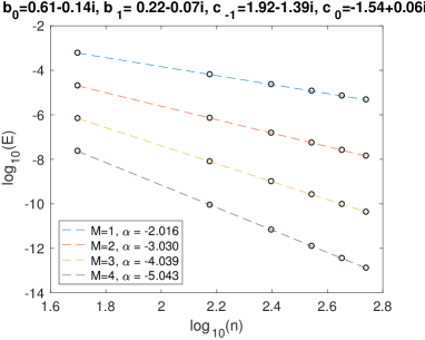
Figure 6.1: Maximum error in estimated eigenvalues. Errors are computed by comparing eigenvalues computed by the proposed method, using a fixed number $M$ of iterations of (6.1), to those computed using the numerical eigenvalue routine eig in MATLAB. Given $\alpha$ values are the slopes of the least-squares linear fits (dotted lines).

Proposition 6.1 implies that, for $N=6n$ , this procedure is guaranteed to find all of the regular eigenvalues of $A$ (provided $n>CD/2$). Before discussing the computational complexity of this procedure, we analyze the iterates of equation (6.1). Theorem 3.12 implies that $|z^{(1)}_{k}-\tilde{z}_{k}|<\frac{CD}{2(1-\Delta)n^{2}}$. Using the bound on $(f^{-1}\circ g)^{\prime}$ from equation (3.3), we see that the later iterates satisfy

$$|z_{k}^{(i)}-\tilde{z}_{k}|<2C\left(\frac{D}{2(1-\Delta)}\right)^{i}\frac{1}{n^{i+1}}.$$ (6.2)

This implies that the residual error in the eigenvalues computed from applying $M$ steps of (6.1) is proportional to $\frac{1}{n^{M+1}}$. This behavior is illustrated in Figure 6.1, where we show the maximum error of the estimated eigenvalues as computed by our method vs $n$, for $n\in\{50,150,250,350,450,550\}$, and $M\in\{1,2,3,4\}$. On a log-log plot, the observed slopes are close to $-(M+1)$, consistent with error proportional to $\frac{1}{n^{M+1}}$.

We now examine the computational complexity of our overall numerical procedure as a function of the matrix size $n$, by counting the number evaluations of either $k(t)$ or $f^{-1}\circ g$ as a proxy for computational cost. Computation of the initial brackets takes $N=6n$ function evaluations. The error from the bisection method after $q$ steps is bounded by $2^{-q}$ times the length of the original bracketing interval, in our case $\frac{2\pi}{6n}$. This implies the need for $q=\log_{2}(\epsilon^{-1})-\log_{2}(3n)$ bisection steps for each phase root, implying a total cost of $6n+(2n+4-2Q)(\log_{2}(\epsilon^{-1})-\log_{2}(3n))$ to compute all of the phase roots. Iterating equation (6.1) for all of the roots requires at most $(2n+4-2Q)M$ function evaluations, where $M$ is the maximum number of iterations performed. The bound (6.2) implies that convergence within $\epsilon$ is assured if $\frac{2C}{n}(\frac{D}{2(1-\Delta)n})^{M}<\epsilon$. Under the conditions $n>2C$ and $n>\frac{D}{(4(1-\Delta)}$, which hold for sufficiently large $n$, convergence within $\epsilon$ is assured for $(\frac{1}{2})^{M}<\epsilon$, which holds for $M=\log_{2}(\epsilon^{-1})$. Thus for sufficiently large $n$, iterating equation (6.1) for all of the roots will require no more than $\log_{2}(\epsilon^{-1})(2n+4-2Q)$ function evaluations. Together, these imply that the total computational cost of computing all of the regular eigenvalues is bounded by $6n+(2n+4-2Q)(2\log_{2}(\epsilon^{-1})$, which is $O(n\log_{2}(\epsilon))$. For $\epsilon$ fixed independent of $n$, the overall computational complexity of our approach is $O(n)$. This should be contrasted with the standard QZ algorithm for computing all of the eigenvalues of a matrix, which has complexity $O(n^{3})$ [8].

Finally, we note that the numerical procedure developed here does not apply to the $Q$ special eigenvalues of $A$, however as these are given by Corollary 5.2 with exponential (in $n$) accuracy, this is not a major limitation.

7 Applications

Matrices like the one we study are often employed in systems of ordinary differential equations. One example of this is in the study of traffic. If one assumes that the acceleration of a car depends linearly on the perception of the relative velocities and positions of the car in front of it and of the car behind it, then some analysis gives rise to the equations

$$\ddot{x}=B_{1}x+B_{2}\dot{x},$$

where $B_{1}$ and $B_{2}$ are matrices of the type given in equation (8.1) with the additional property that they have row sum zero. In the special case that $B_{1}$ and $B_{2}$ are simultaneously diagonalizable, one may use methods similar to those in this paper to study stability (see for example [14]). In the more general case one takes refuge in the method of periodic boundary conditions. This raises the broader question of the mathematical foundation of the validity of that method. Below we make some remarks that relate that question to our present topic.

Discretizations of second order linear partial differential equations (PDE) naturally give rise to tridiagonal matrices similar to the ones in this paper. Below we give an example in 1 dimension. Here we notice that the theory in principle can also be used in certain higher dimensional situations. Suppose we have a linear second order PDE on a rectangle. Then we can discretize horizontally and vertically so that each lattice point interacts with its horizontal neighbors through a matrix, say $L_{1}$, and with its vertical neighbors through $L_{2}$. It is easy to show that the interaction on the entire lattice is given by (see [8], section 4.8)

$$L=L_{1}\otimes I+I\otimes L_{2}$$

where $\otimes$ is the Kronecker product. The eigenvalues of $L$ are give by the Minkowski sum of the eigenvalues of $L_{1}$ and $L_{2}$:

$$\sigma(L)=\{\,z_{1}+z_{2}\,\big{|}\,z_{1}\in\sigma(A_{1}),\;z_{2}\in\sigma(A_{2})\,\},$$

and the eigenvectors are given by the Kronecker product of the eigenvectors of $L_{1}$ and $L_{2}$.

We now make some more detailed comments.

Periodic Boundary Conditions

Perhaps the most common example of periodic boundary conditions is part of the foundation of solid state physics and has many applications in various technologies. A set of identical ions on the line is separated by a distance $a$ (a 1-dimensional Bravais lattice). The position of the ion near $ja$ is denoted by $x_{j}$ and is a function of time. After various approximations, among which the assumption that ion interact only with their nearest neighbors, one arrives at the following equation of motion:

$$\ddot{x}=q(A-2I)x$$ (7.1)

where $q$ is a positive constant related to the strength of the interaction and the mass of the ion. Since physical systems are obviously finite, the remark is then, in the words of [3] (Chapter 22), that “we must specify how the ions at the two ends are to be described. […] but this would complicate the analysis without materially altering the final results. For if $N$ is large then […] the precise way in which the ions at the ends are treated is immaterial […]”. And thus one chooses a convenient way to do that, namely periodic boundary conditions. The idea is clearly that physical bulk — ie no boundary phenomena — properties are unchanged by the use of such boundary conditions. That is: $A_{n+1}-2I$ is replaced by

$$L_{n+1}=\begin{pmatrix}-2&1&0&&\ldots&1\\ 1&-2&1&&\ldots&0\\ \vdots&&\ddots&\ddots&&\vdots\\ 1&\ldots&&0&1&-2\end{pmatrix}\;,$$

so that now:

$$\ddot{x}=qLx\;.$$ (7.2)

To the best of our knowledge, there is no mathematical proof for this important fact at all. It is thus tempting to employ the theory developed here to have a closer look at this.

Write equations (7.1) and (7.2) as linear first order systems. One easily sees that the eigenvalues of those systems are the roots of the eigenvalues of $q(A-2I)$ and of $qL$, respectively. Suppose that the leading eigenvalues of the systems are the most important ones for physical bulk properties. The eigenvalues of $L$ are well-known (and easily derived), namely $2(\cos\frac{2\pi m}{n+1}-1)$. Expanding this to second order and taking the root, we obtain the (approximate) leading eigenvalues for the system of equation (7.2):

$$\nu_{m,\pm}=\pm i\,\frac{2\pi m}{n+1}\quad m\in\{0,1,2,\cdots n\}\;.$$

We expect instabilities to fundamentally influence all physical properties. So if the matrix $A$ in equation (7.1) has an eigenvalue with positive real part whereas the matrix of $L$ in equation (7.2) does not, we can say that periodic boundary conditions fails. That periodic boundary conditions can actually fail in certain circumstances is indicated by the following proposition.

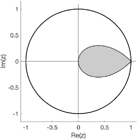
Figure 7.1: Shaded region consists of complex numbers $a+bi$ satisfying $0<a<1$ and $|b|<\sqrt{\frac{a}{2-a}-a^{2}}$ from Theorem 7.1.

Theorem 7.1

Let $r_{1}=a+bi$ be such that $0<a<1$ and $|b|<\sqrt{\frac{a}{2-a}-a^{2}}$, and let $r_{2}\in\mathbb{C}$ arbitrary (see figure 7.1). If the matrix $A$ from equation (1.1) is such that

$$b_{0}=-1/r_{1}-1/r_{2}\mbox{ and }b_{1}=\frac{1}{r_{1}r_{2}},\mbox{ with }c_{0},c_{-1}\mbox{ arbitrary\;, }$$

and$\backslash$or

$$c_{-1}=-1/r_{1}-1/r_{2}\mbox{ and }c_{0}=\frac{1}{r_{1}r_{2}},\mbox{ with }b_{0},b_{1}\mbox{ arbitrary\;, }$$

then for sufficiently large $n$ the system corresponding to equation (7.1) is unstable whereas the system with periodic boundary conditions imposed (equation (7.2)) is Lyapunov stable.

Proof: We have already shown that the eigenvalues of $L$ are negative and thus its roots are imaginary (or 0) which makes the system marginally stable. In fact, the dynamics is that of traveling waves (eg, see [3]), which implies Lyapunov stability.

Assume the first condition holds. Simple algebra shows $(\frac{z}{r_{1}}-1)(\frac{z}{r_{2}}-1)=b_{1}z^{2}+b_{0}z+1$, so $r_{1}$ and $r_{2}$ are the roots of $b_{1}z^{2}+b_{0}z+1$, and are thus also roots of $p(z)$ where $p(z)$ is given in Definition 2.1. As $r_{1}$ is inside the unit circle, Corollary 5.1 implies that $A$ will have an eigenvalue exponentially close to $r_{1}+1/r_{1}$ (as $n\rightarrow\infty$). Simple calculation shows $Re(r_{1}+1/r_{1})=a+\frac{a}{a^{2}+b^{2}}$ and that the inequality $a+\frac{a}{a^{2}+b^{2}}>2$ is equivalent to the conditions on $r_{1}$ given in the hypothesis. These conditions thus imply that the system corresponding to equation (7.1) is unstable. A similar argument applies if the second condition holds.  

More detailed consideration of the notion of periodic boundary conditions can be found in [4], [5], [12], and [11]. However, it is still an open question for what collection $C$ of possible boundary conditions the following holds. For all boundary conditions in $C$, the leading eigenvalues of the Laplacian are (close to) those of the system with periodic boundary conditions. Such a statement would obviously of great value in all kinds of applications. Even in the classical physics case, where the matrices are symmetric, as studied in [6], this problem is to the best of our knowledge unsolved (although the statement is very widely used).

The Advection-Diffusion Equation

We consider a linear advection-diffusion equation on $[0,1]$

$$\partial_{t}u=\partial_{x}^{2}u+2K\partial_{x}u\;,$$ (7.3)

with Dirichlet boundary conditions:

$$u(0,t)=f_{0}(t)\;,\quad u(1,t)=f_{1}(t)\;,$$ (7.4)

and with Dirichlet-Neumann boundary conditions:

$$u(0,t)=f_{0}(t)\;,\quad\partial_{x}u(1,t)=f_{1}(t)\;.$$ (7.5)

Letting $u_{j}(t)$ stand for $u(\frac{j}{n},t)$ and using finite differences (see [9]), one derives the following $n-1$-dimensional (not $n+1$ as in the previous sections) system of ODE. Here $\dot{u}$ indicates derivative with respect to time of $u$. for the system with Dirichlet boundary conditions.

$$\begin{pmatrix}\dot{u}_{1}\\ \dot{u}_{2}\\ \vdots\\ \vdots\\ \dot{u}_{n-1}\\ \end{pmatrix}=n^{2}\,\begin{pmatrix}-2&1+\frac{K}{n}&0&\ldots\\ 1-\frac{K}{n}&-2&1+\frac{K}{n}&\ldots\\ \vdots&\ddots&&\ddots&\vdots\\ &\ldots&1-\frac{K}{n}&-2&1+\frac{K}{n}\\ &\ldots&0&1-\frac{K}{n}&-2\\ \end{pmatrix}\begin{pmatrix}u_{1}\\ u_{2}\\ \vdots\\ \vdots\\ u_{n-1}\\ \end{pmatrix}+n^{2}\,\begin{pmatrix}(1-\frac{K}{n})f_{0}(t)\\ 0\\ \vdots\\ 0\\ (1-\frac{K}{n})f_{1}(t)\\ \end{pmatrix}\;.$$ (7.6)

For the system with Dirichlet-Neumann boundary conditions, we obtain the following $n$ dimensional system.

$$\begin{pmatrix}\dot{u}_{1}\\ \dot{u}_{2}\\ \vdots\\ \vdots\\ \dot{u}_{n}\\ \end{pmatrix}=n^{2}\,\begin{pmatrix}-2&1+\frac{K}{n}&0&\ldots\\ 1-\frac{K}{n}&-2&1+\frac{K}{n}&\ldots\\ \vdots&\ddots&&\ddots&\vdots\\ &\ldots&1-\frac{K}{n}&-2&1+\frac{K}{n}\\ &\ldots&0&2&-2\\ \end{pmatrix}\begin{pmatrix}u_{1}\\ u_{2}\\ \vdots\\ \vdots\\ u_{n}\\ \end{pmatrix}+n^{2}\,\begin{pmatrix}(1-\frac{K}{n})f_{0}(t)\\ 0\\ \vdots\\ 0\\ 2n^{-1}(1+\frac{K}{n})f_{1}(t)\\ \end{pmatrix}\;.$$ (7.7)

The matrix in this equation will be denoted by $B$. In the remainder of this section, we are interested in the eigenvalues of the systems in equations (7.6) and (7.7).

Proposition 7.2

i: Fix $K$. Then for any $n>|K|$, all eigenvalues of the matrix $n^{2}B$ in equation (7.6) are real and less than $-K^{2}$.
ii: Fix $K\leq 0$. Then for any $n>|K|$, all eigenvalues of the matrix $n^{2}B$ in equation (7.7) are real and less than $-K^{2}$.

Proof: The proof of part i follows easily from that of part ii. We start with the latter. First we use Appendix 1 to bring the matrix $B$ in the form used in this paper. Comparison with equation (8.1) shows that

$$q\alpha_{i}^{-1}=1+\frac{K}{n}\;,\;q\alpha_{i}=1-\frac{K}{n}\;,\;\;{\rm and}\;\;qd=-2\;.$$

Solve for $q$, $\alpha_{i}$ and $d$:

$$\alpha_{i}=\alpha\equiv\left(\frac{1-\frac{K}{n}}{1+\frac{K}{n}}\right)^{\frac{1}{2}}\;,q=\left(1-\frac{K^{2}}{n^{2}}\right)^{\frac{1}{2}}\;,\;\;{\rm and}\;\;d=-2\left(1-\frac{K^{2}}{n^{2}}\right)^{-\frac{1}{2}}\;.$$ (7.8)

Defining the diagonal matrix $D$ as in Lemma 8.2, one sees that

$$A\equiv D^{-1}\left(q^{-1}B-dI\right)D=\begin{pmatrix}0&1&0&\ldots\\ 1&0&1&\ldots\\ \vdots&\ddots&&\ddots&\vdots\\ &\ldots&1&0&1\\ &\ldots&0&\frac{2}{1-\frac{K}{n}}&0\end{pmatrix}\;.$$ (7.9)

Comparison with equation (1.1) shows that

$$b_{0}=0\;,\;b_{1}=0\;,\;c_{0}=0\;,\;\;{\rm and}\;\;c_{-1}=1-\frac{2}{1-\frac{K}{n}}=-\frac{1+\frac{K}{n}}{1-\frac{K}{n}}=-\alpha^{-2}\;.$$ (7.10)

Thus the associated polynomial (see Definition 2.1) is:

$$H(z)=z^{2n-2}\,z^{2}\left(c_{-1}+z^{2}\right)-\left(c_{-1}z^{2}+1\right)=z^{2n}\left(z^{2}-\alpha^{-2}\right)-\left(1-\alpha^{-2}z^{2}\right)\;.$$ (7.11)

Re-interpret the polynomial $p(z)=1-\alpha^{-2}z^{2}$ and the auxiliary functions $f$ and $g$ as

$$f(z)=z^{2n}\quad\;\;{\rm and}\;\;\quad g(z)=\frac{p(z)}{z^{2}p(z^{-1})}=\frac{(1-\alpha^{-2}z^{2})}{(z^{2}-\alpha^{-2})}\;.$$ (7.12)

We know from Proposition 3.10 that if $t_{k}$ is a phase root, then $e^{it_{k}}$ is a root of $H(z)$. By Proposition 2.2, the roots $e^{it_{k}}$ of $H(z)/(z^{2}-1)$ correspond to eigenvalues $\lambda_{k}=2\cos(t_{k})$ of $A$. By Corollary 8.3, the corresponding eigenvalues $\nu_{k}$ of $n^{2}B$ are given by:

$$\nu_{k}=n^{2}(q\lambda_{k}+qd)=2n^{2}\left(1-\frac{K^{2}}{n^{2}}\right)^{\frac{1}{2}}\,\cos t_{k}-2n^{2}<-K^{2}\;.$$ (7.13)

Therefore all eigenvalues of $n^{2}B$ arising in this way from roots of $H(z)$ on the unit circle are real numbers less than zero, and no instability arises from them.

When $K=0$, it follows that $\alpha=1$ and $H(z)$ simplifies to

$$H(z)=(z^{2n}+1)(z^{2}-1)\;.$$

Clearly all of the roots of $H(z)/(z^{2}-1)$ lie on the unit circle and none are equal to 1, and so all of the corresponding eigenvalues of $B$ are real numbers less than 0.

When $K<0$, then $\alpha>1$, and $p(z)$ (in equation (7.12)) has no roots inside the unit circle, and so $Q=0$. Adapting the proof of Lemma 3.3 to our re-interpreted $g(z)$ (by recognizing that $g(z)$ is now a rational function of degree 2 rather than of degree 4) shows the winding number of $g$ is $2Q-2$. A similar adaptation of Proposition 3.9 shows that there must be at least $2n+2-2Q=2n+2$ phase roots, each yielding a root of $H(z)$ on the unit circle. But as $H(z)$ is a $2n+2$ degree polynomial, all of the roots of $H(z)$ are on the unit circle and so all of the eigenvalues of $n^{2}B$ are real numbers less than $-K^{2}$.

Now we return to part i. By the same reasoning as before, we now obtain that $c_{-1}$ is also 0. Thus in this case,

$$H(z)=z^{2n}-1\;.$$

The roots of $H$ equal $e^{\frac{\pi ik}{n}}$, and are thus regular. The eigenvalues $\lambda_{k}$ of $A$ equal $\cos\frac{\pi k}{n}$ for $k\in\{1,\cdots n-1\}$ and the corresponding eigenvalues of $n^{2}B$ are less than $-K^{2}$ as follows from equation (7.13).  

We return to the system with mixed boundary conditions. For $K>0$, $p(z)$ in equation (7.12) has precisely 2 roots inside the unit circle. For symmetry reasons, these must be either on the unit circle, in which case the corresponding eigenvalues of $n^{2}B$ are again less than $-K^{2}$, or else the two roots are on the real line. In the latter case, one is the negative of the other. This leads to two special eigenvalues $\lambda$ and $-\lambda$ of $A$, where $\lambda$ is a positive real. By equation (7.13), we see that the eigenvalue of $n^{2}B$ which corresponds to $-\lambda$ will tend to $-\infty$ as $n$ tends to $\infty$, and it is therefore not relevant for the dynamics of the system. One can show that the other special eigenvalue of $n^{2}B$ is always a real number in $(-K^{2},0)$. For brevity, we omit that argument.

Instead we will show that for large positive $K$, the leading eigenvalues of the two systems of equations (7.6) and (7.6) are very different. This is illustrated in figure 7.2. This implies a difference in global dynamics (if given appropriate initial conditions) entirely due to the different boundary conditions.

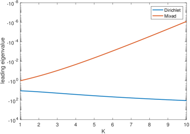
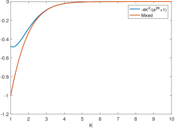
(a)	(b)

Figure 7.2: (a) Leading eigenvalues of $n^{2}B$ for the mixed boundary conditions and the Dirichlet boundary conditions, vs K (note logarithmic scale) (b) Leading eigenvalue of $n^{2}B$ for the mixed boundary condition system, and the prediction from Theorem 7.3, convergence is observed as $K$ increases.

Theorem 7.3

Let $K$ be positive and large. The leading eigenvalue of the system with Dirichlet-Neumann boundary conditions is real and satisfies

$$\nu=-\frac{4K^{2}}{e^{2K}+1}+{\cal O}\left(\frac{K}{\left(e^{2K}+1\right)^{2}}\right)+{\cal O}(n^{-2})\;,$$

while the leading eigenvalue of the system with Dirichlet boundary conditions equals $-K^{2}-\pi^{2}+{\cal O}(n^{-2})$.

Proof: The second part follows immediately from the previous proposition.

Fix a large value of $K$, we locate real roots of $H(z)$ for $n$ arbitrarily large. To do this, set $\zeta\equiv z^{2n}$, $h(\zeta,s)\equiv H(z)$, and $s\equiv 1/n$, then

$$h(\zeta,s)=\zeta\left(\zeta^{s}-\frac{1+Ks}{1-Ks}\right)+\zeta^{s}\frac{1+Ks}{1-Ks}-1\;.$$

The equation for the corresponding eigenvalue of $n^{2}B$ becomes:

$$\nu=s^{-2}\left(\sqrt{1-{K^{2}}{s^{2}}}\,\left(\zeta^{\frac{s}{2}}+\zeta^{-\frac{s}{2}}\right)-2\right)\;.$$

These equations have a meaningful expansions around $s=0$, namely

$$h(\zeta,s)=\left[\zeta(\ln\zeta-2K)+(\ln\zeta+2K)\right]s+{\cal O}(s^{2})\;.$$

Thus, in order for this equation to yield zero near $s=0$, we must have

$$\zeta(\ln\zeta-2K)+(\ln\zeta+2K)=0\quad\;\;{\rm or}\;\;\quad\ln\zeta(\zeta+1)=2K(\zeta-1)\;.$$ (7.14)

The expansion of the second equation (the eigenvalue) is

$$\nu=-K^{2}+\left(\frac{\ln\zeta}{2}\right)^{2}+{\cal O}(s^{2})\;.$$ (7.15)

From equation (7.14) we see that if $K$ is positive and large and $\zeta\in(0,1)$, then $\ln\zeta\approx-2K$, and thus $\zeta$ is very small. We make the following substitution

$$u\equiv\frac{1}{K}\quad\;\;{\rm and}\;\;\quad\mu\equiv-u^{-2}+\left(\frac{\ln\zeta}{2}\right)^{2}\;,$$

and obtain

$$\ln\zeta=2\sqrt{\mu+u^{-2}}\quad\;\;{\rm and}\;\;\quad\zeta=e^{2\sqrt{\mu+u^{-2}}}\;,$$

where $\mu$ is small when $u$ is small. Equation (7.14) becomes:

$$2\sqrt{\mu+u^{-2}}\left(e^{2\sqrt{\mu+u^{-2}}}+1\right)+2u^{-1}\left(1-e^{2\sqrt{\mu+u^{-2}}}\right)=0\;.$$

Multiplying by $\frac{u}{2}$ and rearranging gives:

$$\sqrt{1+\mu u^{2}}=1-\frac{2}{e^{2\sqrt{\mu+u^{-2}}}+1}\;.$$

Note that as $K=u^{-1}$ becomes large, $\mu$ tends to zero exponentially in $K$. Squaring and then subtracting 1, gives

$$\mu u^{2}=-\frac{4}{e^{2\sqrt{\mu+u^{-2}}+1}}+\frac{4}{\left(e^{2\sqrt{\mu+u^{-2}}+1}\right)^{2}}\;.$$ (7.16)

Taylor expand the right hand side of this equation around $\mu=0$. Then substitute the first approximation for $\mu$. Finally, by equation (7.15), $\nu$ and $\mu$ differ by ${\cal O}(n^{-2})$.

The proof of the second statement follows immediately from the proof of part i of Proposition 7.2. Indeed, the reasoning there implies that $\nu_{1}=2n^{2}\left(1-\frac{K^{2}}{n^{2}}\right)^{\frac{1}{2}}\,\cos\frac{\pi}{n}-2n^{2}$ which implies the result.  

8 Appendix 1: More General Form of Matrices

In this appendix we show that with a little work one can expand the class of matrices to which Corollary 5.1 can be applied. Namely, let $d$, $q$, and $\{\alpha_{i}\}_{i=1}^{n}$ be arbitrary complex numbers such that $k$ and $\alpha_{i}$ (for all $i$) are not zero. Define

$${B}_{n+1}=q\begin{pmatrix}d-{b}_{0}&\alpha_{1}^{-1}(1-{b}_{1})&0&&\ldots&0\\ \alpha_{1}&d&\alpha_{2}^{-1}&&\ldots&0\\ 0&\alpha_{2}&d&&\ldots&0\\ \vdots&&\ddots&\ddots&&\vdots\\ 0&\ldots&&\alpha_{n-1}&d&\alpha_{n}^{-1}\\ 0&\ldots&&0&\alpha_{n}(1-{c}_{-1})&d-{c}_{0}\\ \end{pmatrix}.$$ (8.1)

We characterize the eigenpairs of $B$ in terms of those of $A$ given in the main text. For convenience of notation we drop the subscript $n+1$. The following results are simple computations.

Lemma 8.1

Let $D\in{\cal M}$ be the diagonal matrix with $\epsilon_{i}\neq 0$ as its $i$-th diagonal element. Let $M\in{\cal M}$ arbitrary. Then

$$\left(D^{-1}MD\right)_{ij}=\epsilon_{i}^{-1}\epsilon_{j}M_{ij}\;.$$

Lemma 8.2

Set $\epsilon_{i}=\prod_{\ell<i}\,\alpha_{\ell}$ and $\epsilon_{1}=1$, and let $A$ be the matrix given in equation (1.1). Then

$$D^{-1}\left(q^{-1}B-dI\right)D=A\quad\;\;{\rm or}\;\;\quad B=q\left(DAD^{-1}+dI\right)\;.$$

Corollary 8.3

Let $\lambda\in\mathbb{C}$ and $v\in\mathbb{C}^{n+1}$. Then $\left(q(\lambda+d),Dv\right)$ is an eigenpair of $B$ if and only if $(\lambda,v)$ is an eigenpair of $A$.

Remark: In numerical work it is advantageous to work with the matrix $A$ and not with $B$, because $B$ tends to have exponentially large condition number. This expresses itself in the fact that regular eigenvectors $v$ of $A$ tend to have bounded components and, in contrast, the regular eigenvectors $Dv$ of $B$ (see Lemma 8.2) tend to have components whose ratios diverge as $\prod_{\ell<i}\,\alpha_{\ell}$. Clearly this can grow exponentially in $n$, for example if all or most of the $\alpha_{i}>1+c$ and $c>0$.

We briefly mention two examples. Let $T\in{\cal M}$ be the tridiagonal Toeplitz matrix whose diagonal elements equal $\delta$, whose sub-diagonal elements are equal to $\sigma$, and whose super-diagonal elements are equal to to $\tau$. On the other hand, let $A_{0}\in{\cal M}$ be the matrix whose sub- and super-diagonal elements are 1, with $0$ on the diagonal. Corollary 8.3 says that

$$T=\sqrt{\sigma\tau}\,DA_{0}D^{-1}+\delta I.$$

Since the spectrum of $A_{0}$ is easy to derive (namely, $2\cos(\frac{\pi i}{n+2})$ for $i\in\{1,\cdots n+1\}$), the spectrum of $T$ follows immediately (see [13]).

For applications related to consensus forming and flocking, the following matrix was studied in [10]:

$${L}_{n+1}=\begin{pmatrix}\psi&0&0&&\ldots&0\\ \sigma&0&\tau&&\ldots&0\\ 0&\sigma&0&&\ldots&0\\ \vdots&&\ddots&\ddots&&\vdots\\ 0&\ldots&&\sigma&0&\tau\\ 0&\ldots&&0&\sigma+\phi&\theta\\ \end{pmatrix}\;.$$ (8.2)

One sees that $L$ is conjugate to $\tilde{A}$ where

$${\tilde{A}}_{n+1}=\sqrt{\sigma\tau}\,\begin{pmatrix}\frac{\psi}{\sqrt{\sigma\tau}}&0&0&&\ldots&0\\ 1&0&1&&\ldots&0\\ 0&1&0&&\ldots&0\\ \vdots&&\ddots&\ddots&&\vdots\\ 0&\ldots&&1&0&1\\ 0&\ldots&&0&1-\frac{\phi}{\sigma}&\frac{\theta}{\sqrt{\sigma\tau}}\\ \end{pmatrix}\;.$$ (8.3)

The spectrum of $\tilde{A}$ can be studied with the methods of the main text.

References

- [1] L. V. Ahlfors, Complex Analysis, McGraw-Hill, 1979.
- [2] T. M. Apostol, Mathematical Analysis, 2nd edn, Addison-Wesley, 1973.
- [3] N. W. Ashcroft, N.D. Mermin, Solid State Physics, Harcourt, 1976.
- [4] C. E. Cantos, D. K. Hammond, J. J. P. Veerman, Transients in the Synchronization of Oscillator Arrays, European Physical Journal Special Topics 225, 1199-1209, Springer, 2016.
- [5] C. E. Cantos, J. J. P. Veerman, D. K. Hammond, Signal Velocities in Oscillator Networks, European Physical Journal Special Topics, 225, 1115-1126, Springer, 2016.
- [6] C. M. da Fonseca, S. Kouachi, D. A Mazilu, I. Mazilu, A multi-temperature kinetic Ising model and the eigenvalues of some perturbed Jacobi matrices, Applied Mathematics and Computation 259, 205-211, 2015.
- [7] C. M. da Fonseca, J. J. P. Veerman, On the Spectra of Certain Directed Paths, Applied Mathematics Letters 22, 1351-1355, 2009.
- [8] G. H. Golub, C. F. Van Loan, Matrix Computations, 4th Edn, The Johns Hopkins University Press, 2013.
- [9] R. Haberman, Applied Partial Differential Equations, 4th Edn, Pearson-Prentice Hall, 2004.
- [10] J. J. P. Veerman, D, K. Hammond, Tridiagonal Matrices and Boundary Conditions, SIAM Journal of Matrix analysis and Applications, Vol 37, No 1, 1-17, 2016.
- [11] J. Herbrych, A. G. Hazirakis, N. Christakis, J. J. P. Veerman, Dynamics of Locally Coupled Oscillators with Next-Nearest-Neighbor Interaction, Differential Equations and Dynamical Systems, Accepted.
- [12] I. Herman, D. Martinec, and J. J. P. Veerman, Transients of Platoons with Asymmetric and Different Laplacians, Systems & Control Letters, Vol. 91, 28 35, May 2016.
- [13] S. Noschese, L. Pasquini, L. Reichel, Tridiagonal Toeplitz Matrices: Properties and Novel Applications, Numerical Linear Algebra with Applications 20, 302-326, 2013.
- [14] F. M. Tangerman, J. J. P. Veerman, B. D. Stosic, Asymmetric Decentralized Flocks, Transactions on Automatic Control 57, No 11, 2844-2854, 2012.
- [15] W.-C. Yueh, Eigenvalues of Several Tridiagonal Matrices, Applied Mathematics E-Notes 5, 2005, 66-74, 2005.
- [16] D. Kulkarni, D. Schmidt, S.-K. Tsui, Eigenvalues of tridiagonal pseudo-Toeplitz matrices, Linear Algebra and its Applications , Volume 297, Issue 1, 1999