Power spectrum multipoles on the curved sky: an application to the 6-degree Field Galaxy Survey

Abstract

The peculiar velocities of galaxies cause their redshift-space clustering to depend on the angle to the line of sight, providing a key test of gravitational physics on cosmological scales. These effects may be described using a multipole expansion of the clustering measurements. Focussing on Fourier-space statistics, we present a new analysis of the effect of the survey window function, and the variation of the line of sight across a survey, on the modelling of power spectrum multipoles. We determine the joint covariance of the Fourier-space multipoles in a Gaussian approximation, and indicate how these techniques may be extended to studies of overlapping galaxy populations via multipole cross-power spectra. We apply our methodology to one of the widest-area galaxy redshift surveys currently available, the 6-degree Field Galaxy Survey, deducing a normalized growth rate $f\sigma_{8}(z=0.06)=0.38\pm 0.12$ in the low-redshift Universe, in agreement with previous analyses of this dataset using different techniques. Our framework should be useful for processing future wide-angle galaxy redshift surveys.

1 Introduction

The velocities of galaxies within the expanding Universe are generated from underlying density fluctuations by gravitational physics, producing the overall growth of cosmic structure with time. The statistics of these velocities are observable through the correlated Doppler shifts they induce in the galaxy redshifts measured by a spectroscopic survey, known as Redshift-Space Distortions (RSD). This effect imprints an anisotropy in redshift-space galaxy clustering with respect to the local line of sight, which may be used to perform precise tests of gravity on cosmological scales.

The measurement of RSD has become a standard application of modern galaxy redshift surveys (e.g., Blake et al., 2011; Howlett et al., 2015; Alam et al., 2017; Pezzotta et al., 2017), which has allowed the growth rate of structure to be measured with approximately $10\%$ accuracy across the redshift range $z<1$. Standard treatments of RSD clustering statistics exist in both configuration space and Fourier space, featuring various advantages and disadvantages in terms of systematic modelling errors, statistical signal-to-noise and algorithm performance. In this study we develop several new results regarding the application of Fourier-space statistics.

The clustering anisotropy induced by galaxy velocities may be conveniently described by a multipole expansion of the clustering statistics with respect to the local line of sight (Cole et al., 1994; Hamilton, 1998), permitting a powerful compression of the information. The variation of the line-of-sight direction across the survey volume – or “curved-sky” effect – creates complications for algorithms that evaluate Fourier-space clustering statistics using Fast Fourier Transforms (FFTs) (Yamamoto et al., 2006). A series of studies have developed techniques to apply power spectrum multipoles addressing some of the difficulties created by the curved sky (Beutler et al., 2014; Bianchi et al., 2015; Scoccimarro, 2015; Slepian & Eisenstein, 2015a, 2016; Gil-Marín et al., 2016; Wilson et al., 2017; Beutler et al., 2017; Hand et al., 2017; Castorina & White, 2018; Sugiyama et al., 2018). These studies explore estimating multipole power spectra including the effect of the curved sky, modelling multipole power spectra in the presence of a survey window function, applying these algorithms to galaxy surveys (including the suppression of systematics in some modes), and extending these treatments to higher-order statistics such as the bispectrum.

We extend these results in three main areas. First, we present a new technique for evaluating model multipole power spectra in the presence of a survey window function and curved sky. Our method, which is computed purely in Fourier space using FFT-based techniques, is an alternative formulation of the mathematics presented by Wilson et al. (2017) and Beutler et al. (2017). Second, we estimate the joint covariance of power spectrum multipoles using an analytical Gaussian approximation, including window function and curved-sky effects. The covariance of clustering statistics is often determined by applying estimators to a large ensemble of mock catalogues, which are built to match the galaxy survey properties as closely as possible. Whilst this approach enables the inclusion of relevant non-linear effects, realistic mocks may sometimes be difficult to produce in sufficient numbers, causing difficulties in evaluating the likelihood (e.g., Hartlap et al., 2007; Taylor & Joachimi, 2014). Analytical approaches to the covariance are therefore also valuable (e.g., Feldman et al., 1994; Xu et al., 2012; Slepian & Eisenstein, 2015b; O’Connell et al., 2016; Grieb et al., 2016; Mohammed et al., 2017; Hand et al., 2017; Howlett & Percival, 2017). We provide new results that extend the calculations of Feldman et al. (1994) in order to determine the covariance of power spectrum multipoles in the Gaussian approximation, including window function and curved-sky effects. Finally, a number of authors have pointed out that a joint clustering analysis of overlapping galaxy populations, which share correlated sample variance, improves the accuracy of measuring several combinations of cosmological parameters (e.g., McDonald & Seljak, 2009; Gil-Marín et al., 2010; Abramo, 2012; Blake et al., 2013). We extend our convolution and covariance calculations to include the multipole cross-power spectra of overlapping galaxy tracers.

We illustrate some of our new algorithms by performing a multipole power spectrum analysis of one of the widest-area local galaxy redshift surveys, the 6-degree Field Galaxy Survey (6dFGS, Jones et al., 2009). Configuration-space RSD studies of 6dFGS have already been carried out by Beutler et al. (2012) and Achitouv et al. (2017); we present the first Fourier-space treatment. Our techniques should prove useful for the next generation of wide-area spectroscopic studies such as the Taipan Galaxy Survey (da Cunha et al., 2017), the Dark Energy Spectroscopic Instrument (DESI Collaboration et al., 2016) and the 4MOST Cosmology Redshift Survey (de Jong et al., 2012).

Our paper is structured as follows. In Section 2 we introduce the power spectrum multipoles formalism, presenting new calculations regarding the convolution with the survey window function (Section 2.2) and the application to multiple galaxy tracers (Section 2.3), and in Section 3 we develop the analytical covariance in the Gaussian approximation. In Section 4 we present the analysis of 6dFGS data and mocks, and in Section 5 we summarize the results.

2 Power spectrum multipoles formalism

In this Section we summarize a purely Fourier-space scheme to analyze the multipole power spectra of a galaxy redshift survey, including curved-sky effects. We characterize the survey by a window function $\langle n(\textbf{{x}})\rangle$, which predicts the galaxy number density as a function of position in the absence of clustering (with the angle brackets indicating an average over many realizations), and include a position-dependent weight function $w(\textbf{{x}})$ that may be used to optimize the signal-to-noise of the measured statistics.

2.1 Estimating the power spectrum multipoles

We first outline how power spectrum multipoles, $P_{\ell}(k)$, may be estimated from a galaxy distribution. The multipoles are defined by an expansion of the anisotropic galaxy power spectrum $P(\textbf{{k}})$, as a function of wavevector k, with respect to a global line of sight:

$$P(\textbf{{k}})=\sum_{\ell}P_{\ell}(k)\,L_{\ell}(\mu),$$ (1)

where $L_{\ell}$ are Legendre polynomials, and $\mu$ is the cosine of the angle between k and the line of sight (assuming azimuthal symmetry). However, the line-of-sight direction is not fixed, but varies across the galaxy survey. In the region of space around position x, we can write $\mu=\hat{\textbf{{x}}}.\hat{\textbf{{k}}}$ such that for a local line of sight,

$$P(\textbf{{k}},\textbf{{x}})=\sum_{\ell}P_{\ell}(k)\,L_{\ell}(\hat{\textbf{{k}}}.\hat{\textbf{{x}}}).$$ (2)

Inverting Equation 2 and averaging the statistic over all positions, we can evaluate the power spectrum multipoles as

$$P_{\ell}(k)=\frac{2\ell+1}{V}\int d^{3}\textbf{{x}}\int\frac{d\Omega_{k}}{4\pi}\,P(\textbf{{k}},\textbf{{x}})\,L_{\ell}(\hat{\textbf{{k}}}.\hat{\textbf{{x}}}),$$ (3)

where $d\Omega_{k}$ integrates over all angles $\hat{\textbf{{k}}}$. In this formulation we are applying the “local plane-parallel approximation” defined by Beutler et al. (2014), which assumes that the position vectors $(\textbf{{x}},\textbf{{x}}^{\prime})$ of a pair of galaxies separated by relevant scales are locally parallel $(\hat{\textbf{{k}}}.\hat{\textbf{{x}}}\approx\hat{\textbf{{k}}}.\hat{\textbf{{x}}}^{\prime})$, but we account for the changing line-of-sight direction between different pairs. This is a good approximation for our statistics and scales of interest (Pápai & Szapudi, 2008; Samushia et al., 2012; Yoo & Seljak, 2015). Castorina & White (2018) recently presented a systematic exploration of wide-angle effects beyond the local plane-parallel approximation.

We can connect Equation 3 to the distribution of galaxies across space by writing the power spectrum (in standard $h^{-3}$ Mpc³ volume units) as the Fourier transform of the 2-point galaxy correlation function $\xi(\textbf{{x}},\textbf{{x}}^{\prime})=\langle\delta(\textbf{{x}})\,\delta(\textbf{{x}}+\textbf{{s}})\rangle$, as a function of galaxy overdensity $\delta$ and vector separation $\textbf{{s}}=\textbf{{x}}^{\prime}-\textbf{{x}}$, as

$$P(\textbf{{k}},\textbf{{x}})=\int d^{3}\textbf{{s}}\,\xi(\textbf{{x}},\textbf{{x}}^{\prime})\,e^{i\textbf{{k}}.\textbf{{s}}}.$$ (4)

We obtain

$$P_{\ell}(k)=(2\ell+1)\int\frac{d\Omega_{k}}{4\pi}\,\frac{1}{V}\int d^{3}\textbf{{x}}\int d^{3}\textbf{{x}}^{\prime}\,\xi(\textbf{{x}},\textbf{{x}}^{\prime})\,e^{i\textbf{{k}}.(\textbf{{x}}-\textbf{{x}}^{\prime})}\,L_{\ell}(\hat{\textbf{{k}}}.\hat{\textbf{{x}}}^{\prime}).$$ (5)

The form of Equation 5 provides the following estimator for the power spectrum multipoles (Yamamoto et al., 2006; Bianchi et al., 2015; Scoccimarro, 2015):

$$\hat{P}_{\ell}(k)=\frac{2\ell+1}{I}\int\frac{d\Omega_{k}}{4\pi}\left[\frac{1}{V}\int d^{3}\textbf{{x}}\int d^{3}\textbf{{x}}^{\prime}\,\delta_{w}(\textbf{{x}})\,\delta_{w}(\textbf{{x}}^{\prime})\,e^{i\textbf{{k}}.(\textbf{{x}}-\textbf{{x}}^{\prime})}\,L_{\ell}(\hat{\textbf{{k}}}.\hat{\textbf{{x}}}^{\prime})-N_{\ell}(\textbf{{k}})\right],$$ (6)

in terms of the weighted galaxy overdensity $\delta_{w}$ computed from the galaxy density field $n(\textbf{{x}})$,

$$\begin{split}\delta_{w}(\textbf{{x}})&=w(\textbf{{x}})\left[n(\textbf{{x}})-\langle n(\textbf{{x}})\rangle\right]\\ &=w(\textbf{{x}})\,n(\textbf{{x}})-n_{w}(\textbf{{x}}),\end{split}$$ (7)

where $n_{w}(\textbf{{x}})=w(\textbf{{x}})\langle n(\textbf{{x}})\rangle$, the normalization

$$I=\frac{1}{V}\int d^{3}\textbf{{x}}\,n_{w}^{2}(\textbf{{x}}),$$ (8)

and a k-dependent shot noise term that affects all multipoles

$$N_{\ell}(\textbf{{k}})=\frac{1}{V}\int d^{3}\textbf{{x}}\,w^{2}(\textbf{{x}})\,\langle n(\textbf{{x}})\rangle\,L_{\ell}(\hat{\textbf{{k}}}.\hat{\textbf{{x}}}).$$ (9)

These equations agree with those presented in Section 2 of Bianchi et al. (2015) (see also Scoccimarro 2015 and Hand et al. 2017). We refer the reader to Bianchi et al. (2015) for a description of FFT-based methods for evaluating this estimator, which we apply in our analysis.

2.2 Evaluating the model power spectrum multipoles

We now consider how power spectrum multipole model predictions may be evaluated for comparison with these estimators, including the effects of the survey window function and curved sky (in the local plane-parallel approximation). We aim to obtain an expression purely in Fourier co-ordinates, which may be evaluated using FFTs. We evaluate the expectation value $\langle\hat{P}_{\ell}(k)\rangle$ of Equation 6 using (e.g., Feldman et al., 1994)

$$\langle\delta_{w}(\textbf{{x}})\,\delta_{w}(\textbf{{x}}^{\prime})\rangle=w(\textbf{{x}})\,w(\textbf{{x}}^{\prime})\,\langle n(\textbf{{x}})\rangle\,\langle n(\textbf{{x}}^{\prime})\rangle\,\xi(\textbf{{x}},\textbf{{x}}^{\prime})+w^{2}(\textbf{{x}})\,\langle n(\textbf{{x}})\rangle\,\delta_{D}(\textbf{{x}}-\textbf{{x}}^{\prime})/V,$$ (10)

where $\delta_{D}(\textbf{{x}})$ is the Dirac $\delta$-function, normalized such that $(1/V)\int d^{3}\textbf{{x}}\,f(\textbf{{x}})\,\delta_{D}(\textbf{{x}}-\textbf{{x}}_{0})=f(\textbf{{x}}_{0})$. The first and second terms in Equation 10 represent the contribution to the density covariance of sample variance and shot noise, respectively. Substituting Equation 10 in Equation 6 we find

$$\langle\hat{P}_{\ell}(k)\rangle=\frac{2\ell+1}{I}\int\frac{d\Omega_{k}}{4\pi}\,\frac{1}{V}\int d^{3}\textbf{{x}}\,n_{w}(\textbf{{x}})\int d^{3}\textbf{{x}}^{\prime}\,n_{w}(\textbf{{x}}^{\prime})\,\xi(\textbf{{x}},\textbf{{x}}^{\prime})\,e^{i\textbf{{k}}.(\textbf{{x}}-\textbf{{x}}^{\prime})}\,L_{\ell}(\hat{\textbf{{k}}}.\hat{\textbf{{x}}}^{\prime}).$$ (11)

We relate the expectation value $\langle\hat{P}_{\ell}(k)\rangle$ to the underlying model power spectrum statistics using

$$\xi(\textbf{{x}},\textbf{{x}}^{\prime})=\int\frac{d^{3}\textbf{{k}}^{\prime}}{(2\pi)^{3}}\,P(\textbf{{k}}^{\prime},\textbf{{x}}^{\prime})\,e^{-i\textbf{{k}}^{\prime}.(\textbf{{x}}-\textbf{{x}}^{\prime})},$$ (12)

to obtain

$$\langle\hat{P}_{\ell}(k)\rangle=\frac{2\ell+1}{I}\int\frac{d\Omega_{k}}{4\pi}\,\frac{1}{V}\int d^{3}\textbf{{x}}\,n_{w}(\textbf{{x}})\int d^{3}\textbf{{x}}^{\prime}\,n_{w}(\textbf{{x}}^{\prime})\int\frac{d^{3}\textbf{{k}}^{\prime}}{(2\pi)^{3}}\,P(\textbf{{k}}^{\prime},\textbf{{x}}^{\prime})\,e^{i(\textbf{{k}}-\textbf{{k}}^{\prime}).(\textbf{{x}}-\textbf{{x}}^{\prime})}\,L_{\ell}(\hat{\textbf{{k}}}.\hat{\textbf{{x}}}^{\prime}).$$ (13)

Substituting in the multipole expansion of Equation 2 we can write this relation in the form

$$\begin{split}\langle\hat{P}_{\ell}(k)\rangle&=\frac{2\ell+1}{I}\int\frac{d\Omega_{k}}{4\pi}\,\frac{1}{V}\int d^{3}\textbf{{x}}\,n_{w}(\textbf{{x}})\int d^{3}\textbf{{x}}^{\prime}\,n_{w}(\textbf{{x}}^{\prime})\int\frac{d^{3}\textbf{{k}}^{\prime}}{(2\pi)^{3}}\,\sum_{\ell^{\prime}}P_{\ell^{\prime}}(k^{\prime})\,L_{\ell}(\hat{\textbf{{k}}}.\hat{\textbf{{x}}}^{\prime})\,L_{\ell^{\prime}}(\hat{\textbf{{k}}}^{\prime}.\hat{\textbf{{x}}}^{\prime})\,e^{i(\textbf{{k}}-\textbf{{k}}^{\prime}).(\textbf{{x}}-\textbf{{x}}^{\prime})}\\ &=\frac{2\ell+1}{I}\int\frac{d\Omega_{k}}{4\pi}\,\frac{1}{V}\int\frac{d^{3}\textbf{{k}}^{\prime}}{(2\pi)^{3}}\,\sum_{\ell^{\prime}}P_{\ell^{\prime}}(k^{\prime})\,\int d^{3}\textbf{{x}}\,n_{w}(\textbf{{x}})\,e^{i(\textbf{{k}}-\textbf{{k}}^{\prime}).\textbf{{x}}}\int d^{3}\textbf{{x}}^{\prime}\,n_{w}(\textbf{{x}}^{\prime})\,L_{\ell}(\hat{\textbf{{k}}}.\hat{\textbf{{x}}}^{\prime})\,L_{\ell^{\prime}}(\hat{\textbf{{k}}}^{\prime}.\hat{\textbf{{x}}}^{\prime})\,e^{-i(\textbf{{k}}-\textbf{{k}}^{\prime}).\textbf{{x}}^{\prime}}\\ &=\frac{2\ell+1}{I}\int\frac{d\Omega_{k}}{4\pi}\,\sum_{\ell^{\prime}}\frac{V}{(2\pi)^{3}}\int d^{3}\textbf{{k}}^{\prime}\,P_{\ell^{\prime}}(k^{\prime})\,\tilde{n}_{w}(\textbf{{k}}-\textbf{{k}}^{\prime})\,S_{\ell,\ell^{\prime}}^{*}(\textbf{{k}},\textbf{{k}}^{\prime}),\end{split}$$ (14)

where

$$S_{\ell,\ell^{\prime}}(\textbf{{k}},\textbf{{k}}^{\prime})=\frac{1}{V}\int d^{3}\textbf{{x}}\,n_{w}(\textbf{{x}})\,L_{\ell}(\hat{\textbf{{k}}}.\hat{\textbf{{x}}})\,L_{\ell^{\prime}}(\hat{\textbf{{k}}}^{\prime}.\hat{\textbf{{x}}})\,e^{i(\textbf{{k}}-\textbf{{k}}^{\prime}).\textbf{{x}}}.$$ (15)

Physically, $S_{\ell,\ell^{\prime}}(\textbf{{k}},\textbf{{k}}^{\prime})$ describes the effect of the window function in causing a measurement of the multipole power spectrum $P_{\ell}(\textbf{{k}})$ to trace the underlying power on a range of scales $\textbf{{k}}^{\prime}$ and multipoles $\ell^{\prime}$.

We produce a practical algorithm for evaluating $S_{\ell,\ell^{\prime}}(\textbf{{k}},\textbf{{k}}^{\prime})$ by employing the addition theorem for spherical harmonics

$$L_{\ell}(\hat{\textbf{{k}}}.\hat{\textbf{{x}}})=\frac{4\pi}{2\ell+1}\sum_{m=-\ell}^{\ell}Y_{\ell,m}^{*}(\hat{\textbf{{k}}})\,Y_{\ell,m}(\hat{\textbf{{x}}}),$$ (16)

such that

$$S_{\ell,\ell^{\prime}}(\textbf{{k}},\textbf{{k}}^{\prime})=\frac{(4\pi)^{2}}{(2\ell+1)(2\ell^{\prime}+1)}\sum_{m=-\ell}^{\ell}Y^{*}_{\ell,m}(\hat{\textbf{{k}}})\sum_{m^{\prime}=-\ell^{\prime}}^{\ell^{\prime}}Y_{\ell^{\prime},m^{\prime}}(\hat{\textbf{{k}}}^{\prime})\,\tilde{S}_{\ell,m,\ell^{\prime},m^{\prime}}(\textbf{{k}}-\textbf{{k}}^{\prime}),$$ (17)

where

$$\tilde{S}_{\ell,m,\ell^{\prime},m^{\prime}}(\textbf{{k}})=\frac{1}{V}\int d^{3}\textbf{{x}}\,n_{w}(\textbf{{x}})\,Y_{\ell,m}(\hat{\textbf{{x}}})\,Y^{*}_{\ell^{\prime},m^{\prime}}(\hat{\textbf{{x}}})\,e^{i\textbf{{k}}.\textbf{{x}}}.$$ (18)

Hence we obtain the final result

$$\langle\hat{P}_{\ell}(k)\rangle=\frac{1}{I}\int\frac{d\Omega_{k}}{4\pi}\sum_{m=-\ell}^{\ell}Y_{\ell,m}(\hat{\textbf{{k}}})\sum_{\ell^{\prime}}\frac{(4\pi)^{2}}{2\ell^{\prime}+1}\sum_{m^{\prime}=-\ell^{\prime}}^{\ell^{\prime}}\left[\frac{V}{(2\pi)^{3}}\int d^{3}\textbf{{k}}^{\prime}\,P_{\ell^{\prime}}(k^{\prime})\,Y^{*}_{\ell^{\prime},m^{\prime}}(\hat{\textbf{{k}}}^{\prime})\,\tilde{n}_{w}(\textbf{{k}}-\textbf{{k}}^{\prime})\,\tilde{S}^{*}_{\ell,m,\ell^{\prime},m^{\prime}}(\textbf{{k}}-\textbf{{k}}^{\prime})\right].$$ (19)

This relation expresses how the expectation value $\langle\hat{P}_{\ell}(k)\rangle$ mixes the underlying multipole power spectra $P_{\ell^{\prime}}(k^{\prime})$ in a harmonic sum of convolutions involving the survey window function and mixing terms $\tilde{S}_{\ell,m,\ell^{\prime},m^{\prime}}$. The evaluation of the model power spectrum multipoles is hence carried out purely in Fourier space as intended: the formulation of Equation 19 can be evaluated for each $\ell$ using a framework of FFTs by computing $\tilde{S}_{\ell,m,\ell^{\prime},m^{\prime}}(\textbf{{k}})$ using Equation 18, performing a convolution of $P_{\ell^{\prime}}\,Y^{*}_{\ell^{\prime},m^{\prime}}$ and $\tilde{n}_{w}\,\tilde{S}^{*}_{\ell,m,\ell^{\prime},m^{\prime}}$ after distributing $P_{\ell^{\prime}}(k^{\prime})$ on a 3D Fourier grid, summing over multipoles $(m,\ell^{\prime},m^{\prime})$, and averaging the final power spectrum in bins of $k=|\textbf{{k}}|$. In principle the sum over $\ell^{\prime}$ is infinite, but in practice it converges within 2 or 3 terms (which we verify in Section 4.2). If there are $N_{\ell}$ power spectrum multipoles $P_{\ell^{\prime}}(k)$ in the model, the sum over $(m,\ell^{\prime},m^{\prime})$ involves $(2\ell+1)\times N_{\ell}\times(2N_{\ell}-1)$ terms, where each term requires the evaluation of four real-to-complex FFTs.

We check the special case of convolution with a constant window function $n(\textbf{{x}})=n_{0}$ and $w(\textbf{{x}})=1$, for which $\tilde{n}_{w}(\textbf{{k}})=n_{0}\,\tilde{\delta}_{D}(\textbf{{k}})$ where $\tilde{\delta}_{D}(\textbf{{k}})$ is the Dirac $\delta$-function in Fourier space, normalized such that $[V/(2\pi)^{3}]\int\delta^{3}\textbf{{k}}\,\tilde{f}(\textbf{{k}})\,\tilde{\delta}_{D}(\textbf{{k}}-\textbf{{k}}_{0})=\tilde{f}(\textbf{{k}}_{0})$. Substituting this relation in Equation 14 we obtain

$$\langle\hat{P}_{\ell}(k)\rangle=\frac{(2\ell+1)\,n_{0}}{I}\int\frac{d\Omega_{k}}{4\pi}\,\sum_{\ell^{\prime}}P_{\ell^{\prime}}(k)\,S_{\ell,\ell^{\prime}}(\textbf{{k}},\textbf{{k}}),$$ (20)

where, using Equation 15,

$$S_{\ell,\ell^{\prime}}(\textbf{{k}},\textbf{{k}})=\frac{n_{0}}{V}\int d^{3}\textbf{{x}}\,L_{\ell}(\hat{\textbf{{k}}}.\hat{\textbf{{x}}})\,L_{\ell^{\prime}}(\hat{\textbf{{k}}}.\hat{\textbf{{x}}})=\frac{n_{0}\,\delta_{\ell\ell^{\prime}}}{2\ell+1},$$ (21)

by orthogonality of the Legendre polynomials. Since $I=n_{0}^{2}$, we then find $\langle\hat{P}_{\ell}(k)\rangle=P_{\ell}(k)$, as expected in the absence of a survey window function.

Equation 19 is an alternative formulation of the mathematics presented by Wilson et al. (2017) and Beutler et al. (2017), which we derive in Appendix A for completeness. These authors show that the convolved multipole power spectra may be written in the form

$$\langle\hat{P}_{\ell}(k)\rangle=4\pi\,i^{\ell}\int ds\,s^{2}\,j_{\ell}(ks)\,\hat{\xi}_{\ell}(s),$$ (22)

where $j_{\ell}$ are the spherical Bessel functions and

$$\hat{\xi}_{\ell}(s)=(2\ell+1)\sum_{\ell^{\prime}}\xi_{\ell^{\prime}}(s)\sum_{\ell^{\prime\prime}}A^{\ell^{\prime\prime}}_{\ell,\ell^{\prime}}\,\frac{W_{\ell^{\prime\prime}}^{2}(s)}{2\ell^{\prime\prime}+1},$$ (23)

is written in terms of the model correlation function multipoles $\xi_{\ell}$, coefficients $A^{\ell^{\prime\prime}}_{\ell,\ell^{\prime}}$ listed in Equation 66, and window function multipoles

$$W_{\ell}^{2}(s)=\frac{2\ell+1}{I}\int\frac{d\Omega_{s}}{4\pi}\,\frac{1}{V}\int d^{3}\textbf{{x}}\,n_{w}(\textbf{{x}})\,n_{w}(\textbf{{x}}+\textbf{{s}})\,L_{\ell}(\hat{\textbf{{x}}}.\hat{\textbf{{s}}}).$$ (24)

Wilson et al. (2017) and Beutler et al. (2017) recommend evaluating $W_{\ell}^{2}$ in bins of separation $s$ of width $\Delta s$ using a pair count over a random catalogue, where each pair $(\textbf{{x}},\textbf{{x}}^{\prime})$ is weighted in proportion to $w(\textbf{{x}})\,w(\textbf{{x}}^{\prime})\,L_{\ell}(\textbf{{x}}.\textbf{{s}})/s^{2}\,\Delta s$. Alternatively, using the FFT-based formalism of our study to avoid the pair count, we can evaluate the window function multipoles by writing Equation 24 in the form

$$W_{\ell}^{2}(s)=\frac{2\ell+1}{I}\int\frac{d\Omega_{s}}{4\pi}\,\frac{1}{V}\int d^{3}\textbf{{x}}\,n_{w}(\textbf{{x}})\,\frac{V}{(2\pi)^{3}}\int d^{3}\textbf{{k}}\,\tilde{n}_{w}^{*}(\textbf{{k}})\,e^{i\textbf{{k}}.\textbf{{x}}}\,e^{i\textbf{{k}}.\textbf{{s}}}\,L_{\ell}(\hat{\textbf{{x}}}.\hat{\textbf{{s}}}).$$ (25)

We produce a practical algorithm for evaluating this expression by employing the plane-wave expansion

$$e^{i\textbf{{k}}.\textbf{{s}}}=\sum_{\ell}i^{\ell}\,(2\ell+1)\,j_{\ell}(ks)\,L_{\ell}(\hat{\textbf{{k}}}.\hat{\textbf{{s}}}),$$ (26)

to derive the new relation

$$W_{\ell}^{2}(s)=\frac{4\pi\,i^{\ell}}{I}\sum_{m=-\ell}^{\ell}\frac{V}{(2\pi)^{3}}\int d^{3}\textbf{{k}}\,\tilde{n}_{w}^{*}(\textbf{{k}})\,j_{\ell}(ks)\,Y_{\ell,m}(\hat{\textbf{{k}}})\,\frac{1}{V}\int d^{3}\textbf{{x}}\,n_{w}(\textbf{{x}})\,Y_{\ell,m}^{*}(\hat{\textbf{{x}}})\,e^{i\textbf{{k}}.\textbf{{x}}}.$$ (27)

This expression may be evaluated for given $\ell$ and $s$ by computing the FFT of $n_{w}(\textbf{{x}})\,Y_{\ell,m}^{*}(\hat{\textbf{{x}}})$, and summing the product of functions over k-space, for each $m$. We note that this is the generalization of Equation 20 of Wilson et al. (2017), which applies in the flat-sky approximation. The two formulations are identical for $\ell=0$.

Multipole power spectrum estimates may be corrected to satisfy the integral constraint condition, which can be evaluated as described by Section A2 of Beutler et al. (2017). The correction is typically negligible on the scales of interest.

2.3 Cross-power spectrum multipoles with overlapping tracers

The preceding formulation may be extended to the analysis of spatially-overlapping galaxy populations via their cross-power spectrum (see also, Smith, 2009; Blake et al., 2013). The generalization of Equation 6 to the estimation of the cross-power spectrum multipoles $P_{\ell,c}(k)$ of two tracers with number densities $n_{1}(\textbf{{x}})$ and $n_{2}(\textbf{{x}})$, with respective weight functions $w_{1}(\textbf{{x}})$ and $w_{2}(\textbf{{x}})$, is given by

$$\hat{P}_{\ell,c}(k)=\frac{2\ell+1}{I_{c}}\int\frac{d\Omega_{k}}{4\pi}\frac{1}{V}\int d^{3}\textbf{{x}}\int d^{3}\textbf{{x}}^{\prime}\,\frac{1}{2}\left[\delta_{1,w}(\textbf{{x}})\,\delta_{2,w}(\textbf{{x}}^{\prime})+\delta_{2,w}(\textbf{{x}})\,\delta_{1,w}(\textbf{{x}}^{\prime})\right]L_{\ell}(\hat{\textbf{{k}}}.\hat{\textbf{{x}}}^{\prime})\,e^{i\textbf{{k}}.(\textbf{{x}}-\textbf{{x}}^{\prime})},$$ (28)

in terms of the weighted overdensities

$$\delta_{i,w}(\textbf{{x}})=w_{i}(\textbf{{x}})\left[n_{i}(\textbf{{x}})-\langle n_{i}(\textbf{{x}})\rangle\right],$$ (29)

where $i=\{1,2\}$ denotes the tracer, and the normalization of the cross-power spectrum

$$I_{c}=\frac{1}{V}\int d^{3}\textbf{{x}}\,w_{1}(\textbf{{x}})\,w_{2}(\textbf{{x}})\,\langle n_{1}(\textbf{{x}})\rangle\,\langle n_{2}(\textbf{{x}})\rangle.$$ (30)

We note that Equation 28 is constructed to be symmetric under interchange of the indices 1 and 2, and that there is no shot noise contribution to the cross-power spectrum. We estimate the cross-power spectrum multipoles using a lightly-modified version of the method of Bianchi et al. (2015). We can evaluate the expectation value of Equation 28 using

$$\langle\delta_{1,w}(\textbf{{x}})\,\delta_{2,w}(\textbf{{x}}^{\prime})\rangle=w_{1}(\textbf{{x}})\,w_{2}(\textbf{{x}}^{\prime})\,\langle n_{1}(\textbf{{x}})\rangle\,\langle n_{2}(\textbf{{x}}^{\prime})\rangle\,\xi_{12}(\textbf{{x}},\textbf{{x}}^{\prime}),$$ (31)

where $\xi_{12}$ is the cross-correlation function of the tracers, which is related to their cross-power spectrum in the same manner as Equation 12. Proceeding with a similar derivation as in Section 2.2 we find

$$\langle\hat{P}_{\ell,c}(k)\rangle=\frac{1}{I_{c}}\int\frac{d\Omega_{k}}{4\pi}\sum_{m=-\ell}^{\ell}Y_{\ell,m}(\hat{\textbf{{k}}})\sum_{\ell^{\prime}}\frac{(4\pi)^{2}}{2\ell^{\prime}+1}\sum_{m^{\prime}=-\ell^{\prime}}^{\ell^{\prime}}\left[\left(P_{\ell^{\prime},c}\,Y^{*}_{\ell^{\prime},m^{\prime}}\right)\star\frac{1}{2}\left(\tilde{n}_{2,w}\,\tilde{S}^{1*}_{\ell,m,\ell^{\prime},m^{\prime}}+\tilde{n}_{1,w}\,\tilde{S}^{2*}_{\ell,m,\ell^{\prime},m^{\prime}}\right)\right],$$ (32)

where $n_{i,w}(\textbf{{x}})=w_{i}(\textbf{{x}})\,\langle n_{i}(\textbf{{x}})\rangle$, $\tilde{S}^{i}_{\ell,m,\ell^{\prime},m^{\prime}}$ is given by Equation 18 with $n_{w}=n_{i,w}$, and $\star$ denotes convolution.

3 Covariance of the power spectrum multipoles

In this Section we formulate analytical expressions for the covariance of the power spectrum multipole estimates described in Section 2.1, between different multipoles and scales. Feldman et al. (1994) derive the covariance of the estimated galaxy power spectrum

$$\langle\delta\hat{P}(k)\,\delta\hat{P}(k^{\prime})\rangle=\left\langle\left(\hat{P}(k)-\langle\hat{P}(k)\rangle\right)\left(\hat{P}(k^{\prime})-\langle\hat{P}(k^{\prime})\rangle\right)\right\rangle=\langle\hat{P}(k)\,\hat{P}(k^{\prime})\rangle-\langle\hat{P}(k)\rangle\langle\hat{P}(k^{\prime})\rangle,$$ (33)

in the approximation that the galaxy overdensity is a Gaussian random field sampled by Poisson statistics. We use similar methods to determine analogous expressions for the joint covariance of the multipole power spectra, extending the calculations of Taruya et al. (2010), Grieb et al. (2016) and Hand et al. (2017) to account for window function and curved-sky effects (in the local plane-parallel approximation).

We note that the covariance may be impacted by various non-Gaussian effects, such as higher-order correlations (trispectrum terms) (e.g. O’Connell et al., 2016; Howlett & Percival, 2017) or non-Poisson sampling of the density field by galaxies (e.g. Seljak et al., 2009; Baldauf et al., 2013; Ginzburg et al., 2017). However, Gaussian approximations may serve a valuable purpose on large scales, or when simulations are not available to calibrate these effects sufficiently.

The covariance between power spectrum multipoles $(\ell,\ell^{\prime})$ averaged in spherical shells around wavenumbers $(k,k^{\prime})$ may be determined as

$$\langle\delta\hat{P}_{\ell}(k)\,\delta\hat{P}_{\ell^{\prime}}(k^{\prime})\rangle=\int\frac{d\Omega_{k}}{4\pi}\int\frac{d\Omega_{k^{\prime}}}{4\pi}\langle\delta\hat{P}_{\ell}(\textbf{{k}})\,\delta\hat{P}_{\ell^{\prime}}(\textbf{{k}}^{\prime})\rangle,$$ (34)

where, using the estimator of Equation 6,

$$\begin{split}\langle\delta\hat{P}_{\ell}(\textbf{{k}})\,\delta\hat{P}_{\ell^{\prime}}(\textbf{{k}}^{\prime})\rangle=\frac{(2\ell+1)\,(2\ell^{\prime}+1)}{V^{2}\,I^{2}}&\int d^{3}\textbf{{x}}_{1}\int d^{3}\textbf{{x}}_{2}\int d^{3}\textbf{{x}}_{3}\int d^{3}\textbf{{x}}_{4}\,e^{i\textbf{{k}}.(\textbf{{x}}_{1}-\textbf{{x}}_{2})}\,e^{i\textbf{{k}}^{\prime}.(\textbf{{x}}_{3}-\textbf{{x}}_{4})}\,L_{\ell}(\hat{\textbf{{k}}}.\hat{\textbf{{x}}}_{2})\,L_{\ell^{\prime}}(\hat{\textbf{{k}}}^{\prime}.\hat{\textbf{{x}}}_{4})\\ &\left[\langle\delta_{w}(\textbf{{x}}_{1})\,\delta_{w}(\textbf{{x}}_{2})\,\delta_{w}(\textbf{{x}}_{3})\,\delta_{w}(\textbf{{x}}_{4})\rangle-\langle\delta_{w}(\textbf{{x}}_{1})\,\delta_{w}(\textbf{{x}}_{2})\rangle\langle\delta_{w}(\textbf{{x}}_{3})\,\delta_{w}(\textbf{{x}}_{4})\rangle\right].\end{split}$$ (35)

We apply the Gaussian approximation using Wick’s theorem for a Gaussian random field

$$\langle\delta_{1}\,\delta_{2}\,\delta_{3}\,\delta_{4}\rangle=\langle\delta_{1}\,\delta_{2}\rangle\langle\delta_{3}\,\delta_{4}\rangle+\langle\delta_{1}\,\delta_{3}\rangle\langle\delta_{2}\,\delta_{4}\rangle+\langle\delta_{1}\,\delta_{4}\rangle\langle\delta_{2}\,\delta_{3}\rangle,$$ (36)

which (omitting some algebra) allows us to write the covariance in the form

$$\langle\delta\hat{P}_{\ell}(\textbf{{k}})\,\delta\hat{P}_{\ell^{\prime}}(\textbf{{k}}^{\prime})\rangle=\frac{(2\ell+1)\,(2\ell^{\prime}+1)}{I^{2}}\left[C_{\ell,\ell^{\prime}}(\textbf{{k}},\textbf{{k}}^{\prime})\,C_{0,0}(\textbf{{k}},\textbf{{k}}^{\prime})^{*}+C_{\ell,0}(\textbf{{k}},\textbf{{k}}^{\prime})\,C_{0,\ell^{\prime}}(\textbf{{k}},\textbf{{k}}^{\prime})^{*}\right],$$ (37)

where

$$C_{\ell,\ell^{\prime}}(\textbf{{k}},\textbf{{k}}^{\prime})=\frac{1}{V}\int d^{3}\textbf{{x}}\int d^{3}\textbf{{x}}^{\prime}\,\langle\delta_{w}(\textbf{{x}})\,\delta_{w}(\textbf{{x}}^{\prime})\rangle\,e^{i(\textbf{{k}}.\textbf{{x}}-\textbf{{k}}^{\prime}.\textbf{{x}}^{\prime})}\,L_{\ell}(\hat{\textbf{{k}}}.\hat{\textbf{{x}}})\,L_{\ell^{\prime}}(\hat{\textbf{{k}}}^{\prime}.\hat{\textbf{{x}}}^{\prime}).$$ (38)

We evaluate this expression by substituting in Equations 10 and 12 with the additional approximation that the covariance between two scales k and $\textbf{{k}}^{\prime}$ may be determined by the clustering power at those scales, rather than by all modes (i.e., for the purposes of evaluating the covariance, neglecting convolution). This approximation is necessary to allow the covariance to be expressed as a single integral over space, which may be evaluated by FFTs. We find

$$C_{\ell,\ell^{\prime}}(\textbf{{k}},\textbf{{k}}^{\prime})\approx\frac{1}{V}\int d^{3}\textbf{{x}}\,w^{2}(\textbf{{x}})\,\left[n^{2}(\textbf{{x}})\,P_{\rm eff}(\textbf{{k}},\textbf{{k}}^{\prime},\textbf{{x}})+n(\textbf{{x}})\right]e^{i(\textbf{{k}}-\textbf{{k}}^{\prime}).\textbf{{x}}}\,L_{\ell}(\hat{\textbf{{k}}}.\hat{\textbf{{x}}})\,L_{\ell^{\prime}}(\hat{\textbf{{k}}}^{\prime}.\hat{\textbf{{x}}}),$$ (39)

where, in order to preserve the symmetry of the covariance $C_{\ell,\ell}(\textbf{{k}},\textbf{{k}}^{\prime})=C_{\ell,\ell}(\textbf{{k}}^{\prime},\textbf{{k}})$, we use an effective power spectrum

$$P_{\rm eff}(\textbf{{k}},\textbf{{k}}^{\prime},\textbf{{x}})=\frac{1}{2}\sum_{\ell^{\prime\prime}}\left[P_{\ell^{\prime\prime}}(k)\,L_{\ell^{\prime\prime}}(\hat{\textbf{{k}}}.\hat{\textbf{{x}}})+P_{\ell^{\prime\prime}}(k^{\prime})\,L_{\ell^{\prime\prime}}(\hat{\textbf{{k}}}^{\prime}.\hat{\textbf{{x}}})\right],$$ (40)

in place of Equation 2. In physical terms, Equation 39 represents a combination of sample variance and shot noise contributions, respectively $C^{SV}$ and $C^{SN}$, corresponding to the two terms inside the square bracket. In practice we restrict the sum over $\ell^{\prime\prime}$ to the monopole and quadrupole.

We illustrate our method for evaluating Equation 39 using the first term, $P_{\rm eff}=\sum_{\ell^{\prime\prime}}P_{\ell^{\prime\prime}}(k)\,L_{\ell^{\prime\prime}}(\hat{\textbf{{k}}}.\hat{\textbf{{x}}})$. Its contribution to the sample variance covariance is

$$C^{SV}_{\ell,\ell^{\prime}}(\textbf{{k}},\textbf{{k}}^{\prime})=\sum_{\ell^{\prime\prime}}P_{\ell^{\prime\prime}}(k)\,\frac{1}{V}\int d^{3}\textbf{{x}}\,n_{w}^{2}(\textbf{{x}})\,L_{\ell^{\prime\prime}}(\hat{\textbf{{k}}}.\hat{\textbf{{x}}})\,L_{\ell}(\hat{\textbf{{k}}}.\hat{\textbf{{x}}})\,L_{\ell^{\prime}}(\hat{\textbf{{k}}}^{\prime}.\hat{\textbf{{x}}})\,e^{i(\textbf{{k}}-\textbf{{k}}^{\prime}).\textbf{{x}}}.$$ (41)

Using Equation 66 this can be written in the form

$$C^{SV}_{\ell,\ell^{\prime}}(\textbf{{k}},\textbf{{k}}^{\prime})=\sum_{\ell^{\prime\prime}}P_{\ell^{\prime\prime}}(k)\sum_{\ell^{\prime\prime\prime}}A_{\ell,\ell^{\prime\prime}}^{\ell^{\prime\prime\prime}}\frac{(4\pi)^{2}}{(2\ell^{\prime\prime\prime}+1)(2\ell^{\prime}+1)}\sum_{m^{\prime\prime\prime}=-\ell^{\prime\prime\prime}}^{\ell^{\prime\prime\prime}}\sum_{m^{\prime}=-\ell^{\prime}}^{\ell^{\prime}}Y^{*}_{\ell^{\prime\prime\prime},m^{\prime\prime\prime}}(\hat{\textbf{{k}}})\,Y_{\ell^{\prime},m^{\prime}}(\hat{\textbf{{k}}}^{\prime})\,\tilde{Q}_{\ell^{\prime\prime\prime},m^{\prime\prime\prime},l^{\prime},m^{\prime}}(\textbf{{k}}-\textbf{{k}}^{\prime}),$$ (42)

where

$$\tilde{Q}_{\ell,m,\ell^{\prime},m^{\prime}}(\textbf{{k}})=\frac{1}{V}\int d^{3}\textbf{{x}}\,n_{w}^{2}(\textbf{{x}})\,Y_{\ell,m}(\hat{\textbf{{x}}})\,Y^{*}_{\ell^{\prime},m^{\prime}}(\hat{\textbf{{x}}})\,e^{i\textbf{{k}}.\textbf{{x}}}.$$ (43)

This covariance contribution $C^{SV}$ quantifies how the underlying power spectrum drives sample variance, which is correlated across scales by the window function $\tilde{Q}$. Likewise for the shot noise contribution:

$$C^{SN}_{\ell,\ell^{\prime}}(\textbf{{k}},\textbf{{k}}^{\prime})=\frac{1}{V}\int d^{3}\textbf{{x}}\,n_{w}(\textbf{{x}})\,L_{\ell}(\hat{\textbf{{k}}}.\hat{\textbf{{x}}})\,L_{\ell^{\prime}}(\hat{\textbf{{k}}}^{\prime}.\hat{\textbf{{x}}})\,e^{i(\textbf{{k}}-\textbf{{k}}^{\prime}).\textbf{{x}}}=\frac{(4\pi)^{2}}{(2\ell+1)(2\ell^{\prime}+1)}\sum_{m=-\ell}^{\ell}\sum_{m^{\prime}=-\ell^{\prime}}^{\ell^{\prime}}Y^{*}_{\ell,m}(\hat{\textbf{{k}}})\,Y_{\ell^{\prime},m^{\prime}}(\hat{\textbf{{k}}}^{\prime})\,\tilde{S}_{\ell,m,l^{\prime},m^{\prime}}(\textbf{{k}}-\textbf{{k}}^{\prime}),$$ (44)

where $\tilde{S}_{\ell,m,l^{\prime},m^{\prime}}$ is defined by Equation 18. This hence provides an FFT-based framework for evaluating the covariance in the Gaussian approximation, by first computing $\tilde{S}_{\ell,m,\ell^{\prime},m^{\prime}}(\textbf{{k}})$ and $\tilde{Q}_{\ell,m,\ell^{\prime},m^{\prime}}(\textbf{{k}})$ using Equations 18 and 43 and then performing sums over spherical harmonic coefficients. Our development has hence reduced the dimensionality of the covariance calculation from a multiple integral over four 3D spaces in Equation 35, to a harmonic sum of terms sampled within a single k-space.

It is useful to consider some special cases. For a constant window function $n(\textbf{{x}})=n_{0}$ and $w(\textbf{{x}})=1$, the appearance of the position-dependent Legendre polynomials inside Equation 41 implies that there are still correlations between multipole power spectra $P_{\ell}(\textbf{{k}})$ with different $\ell$ and k. This is unlike the case of a global flat-sky approximation relative to an axis $\hat{\textbf{{x}}}_{0}$, for which the Legendre polynomials in Equation 41 take the form $L_{\ell}(\hat{\textbf{{k}}}.\hat{\textbf{{x}}}_{0})$ and the integral over x becomes a Dirac $\delta$-function, removing the k-correlations. Another useful special case is an isotropic window function, for which Equation 43 can be written

$$\tilde{Q}_{\ell,m,\ell^{\prime},m^{\prime}}(0)=\frac{1}{V}\int dr\,r^{2}\,n_{w}^{2}(r)\int d\Omega\,Y_{\ell,m}(\hat{\textbf{{x}}})\,Y^{*}_{\ell^{\prime},m^{\prime}}(\hat{\textbf{{x}}})=\frac{1}{V}\int dr\,r^{2}\,n_{w}^{2}(r)\,\delta_{\ell,\ell^{\prime}}\delta_{m,m^{\prime}},$$ (45)

using the orthonormality of the spherical harmonics. Using this result in Equation 42 with $\textbf{{k}}^{\prime}=\textbf{{k}}$, we find

$$C^{SV}_{\ell,\ell^{\prime}}(\textbf{{k}},\textbf{{k}})=\frac{1}{V}\int dr\,r^{2}\,n_{w}^{2}(r)\sum_{\ell^{\prime\prime}}P_{\ell^{\prime\prime}}(k)\,\left(\begin{matrix}\ell&\ell^{\prime\prime}&\ell^{\prime}\\ 0&0&0\end{matrix}\right)$$ (46)

where $\left(\begin{matrix}\ell&\ell^{\prime\prime}&\ell^{\prime}\\ 0&0&0\end{matrix}\right)$ is a Wigner 3j-symbol.

For a general window function we have not found any further simplications, but the terms are straight-forward to evaluate numerically. In practice we carry out the required average by randomly sub-sampling modes k and $\textbf{{k}}^{\prime}$ in spherical shells around wavenumbers $k$ and $k^{\prime}$, separately treating the case $\textbf{{k}}^{\prime}=\textbf{{k}}$. We randomly choose (a maximum of) 100 modes in each bin to perform this calculation, checking that our results are not sensitive to this choice. For example, to determine the contribution of Equation 42 to the first covariance term we compute

$$\int\frac{d\Omega_{k}}{4\pi}\int\frac{d\Omega_{k^{\prime}}}{4\pi}\,C^{SV}_{\ell,\ell^{\prime}}(\textbf{{k}},\textbf{{k}}^{\prime})\,C_{0,0}(\textbf{{k}},\textbf{{k}}^{\prime})^{*}=\sum_{\ell^{\prime\prime}}P_{\ell^{\prime\prime}}(k)\sum_{\ell^{\prime\prime\prime}}A_{\ell,\ell^{\prime\prime}}^{\ell^{\prime\prime\prime}}\frac{(4\pi)^{2}}{(2\ell^{\prime\prime\prime}+1)(2\ell^{\prime}+1)}\sum_{m^{\prime\prime\prime}}\sum_{m^{\prime}}\left[P_{0}(k^{\prime})\,\overline{QQ}(k,k^{\prime})+\overline{QS}(k,k^{\prime})\right],$$ (47)

where

$$\begin{split}\overline{QQ}(k,k^{\prime})&=\overline{Y^{*}_{\ell,m}(\hat{\textbf{{k}}})\,Y_{\ell^{\prime},m^{\prime}}(\hat{\textbf{{k}}}^{\prime})\,\tilde{Q}_{\ell,m,\ell^{\prime},m^{\prime}}(\textbf{{k}}-\textbf{{k}}^{\prime})\,\tilde{Q}^{*}_{0,0,0,0}(\textbf{{k}}-\textbf{{k}}^{\prime})}\\ \overline{QS}(k,k^{\prime})&=\overline{Y^{*}_{\ell,m}(\hat{\textbf{{k}}})\,Y_{\ell^{\prime},m^{\prime}}(\hat{\textbf{{k}}}^{\prime})\,\tilde{Q}_{\ell,m,\ell^{\prime},m^{\prime}}(\textbf{{k}}-\textbf{{k}}^{\prime})\,\tilde{S}^{*}_{0,0,0,0}(\textbf{{k}}-\textbf{{k}}^{\prime})},\end{split}$$ (48)

where the overbar denotes an average over a sub-sample of modes. We derive similar expressions for the remaining terms.

In a multi-tracer analysis, we can also develop the remaining expressions for the covariances of the auto- and cross-power spectrum multipoles in the Gaussian approximation, i.e., $\langle\hat{P}_{\ell,1}(k)\,\hat{P}_{\ell^{\prime},2}(k^{\prime})\rangle$, $\langle\hat{P}_{\ell,1}(k)\,\hat{P}_{\ell^{\prime},c}(k^{\prime})\rangle$ and $\langle\hat{P}_{\ell,c}(k)\,\hat{P}_{\ell^{\prime},c}(k^{\prime})\rangle$. For example, the first of these covariances can be evaluated by averaging in $k$-space shells the quantity

$$\langle\delta\hat{P}_{\ell,1}(\textbf{{k}})\,\delta\hat{P}_{\ell^{\prime},2}(\textbf{{k}}^{\prime})\rangle=\frac{(2\ell+1)\,(2\ell^{\prime}+1)}{I_{1}\,I_{2}}\left[C^{12}_{\ell,\ell^{\prime}}(\textbf{{k}},\textbf{{k}}^{\prime})\,C^{12}_{0,0}(\textbf{{k}},\textbf{{k}}^{\prime})^{*}+C^{12}_{\ell,0}(\textbf{{k}},\textbf{{k}}^{\prime})\,C^{12}_{0,\ell^{\prime}}(\textbf{{k}},\textbf{{k}}^{\prime})^{*}\right],$$ (49)

where

$$C^{12}_{\ell,\ell^{\prime}}(\textbf{{k}},\textbf{{k}}^{\prime})\approx\frac{1}{V}\int d^{3}\textbf{{x}}\,n_{1,w}(\textbf{{x}})\,n_{2,w}(\textbf{{x}})\,P_{c}(\textbf{{k}},\textbf{{k}}^{\prime},\textbf{{x}})\,e^{i(\textbf{{k}}-\textbf{{k}}^{\prime}).\textbf{{x}}}\,L_{\ell}(\hat{\textbf{{k}}}.\hat{\textbf{{x}}})\,L_{\ell^{\prime}}(\hat{\textbf{{k}}}^{\prime}.\hat{\textbf{{x}}}).$$ (50)

Using the same methods as above, the equivalent of Equation 42 is

$$C^{12}_{\ell,\ell^{\prime}}(\textbf{{k}},\textbf{{k}}^{\prime})=\sum_{\ell^{\prime\prime}}P_{c,\ell^{\prime\prime}}(k)\sum_{\ell^{\prime\prime\prime}}A_{\ell,\ell^{\prime\prime}}^{\ell^{\prime\prime\prime}}\frac{(4\pi)^{2}}{(2\ell^{\prime\prime\prime}+1)(2\ell^{\prime}+1)}\sum_{m^{\prime\prime\prime}}\sum_{m^{\prime}}Y^{*}_{\ell^{\prime\prime\prime},m^{\prime\prime\prime}}(\hat{\textbf{{k}}})\,Y_{\ell^{\prime},m^{\prime}}(\hat{\textbf{{k}}}^{\prime})\,\tilde{Q}^{12}_{\ell^{\prime\prime\prime},m^{\prime\prime\prime},l^{\prime},m^{\prime}}(\textbf{{k}}-\textbf{{k}}^{\prime}),$$ (51)

where

$$\tilde{Q}^{12}_{\ell,m,\ell^{\prime},m^{\prime}}(\textbf{{k}})=\frac{1}{V}\int d^{3}\textbf{{x}}\,n_{1,w}(\textbf{{x}})\,n_{2,w}(\textbf{{x}})\,Y_{\ell,m}(\hat{\textbf{{x}}})\,Y^{*}_{\ell^{\prime},m^{\prime}}(\hat{\textbf{{x}}})\,e^{i\textbf{{k}}.\textbf{{x}}}.$$ (52)

As before, we numerically compute the average by randomly sub-sampling modes k and $\textbf{{k}}^{\prime}$ in spherical shells around wavenumbers $k$ and $k^{\prime}$:

$$\int\frac{d\Omega_{k}}{4\pi}\int\frac{d\Omega_{k^{\prime}}}{4\pi}\,C^{12}_{\ell,\ell^{\prime}}(\textbf{{k}},\textbf{{k}}^{\prime})\,C^{12}_{0,0}(\textbf{{k}},\textbf{{k}}^{\prime})^{*}=\sum_{\ell^{\prime\prime}}P_{c,\ell^{\prime\prime}}(k)\sum_{\ell^{\prime\prime\prime}}A_{\ell,\ell^{\prime\prime}}^{\ell^{\prime\prime\prime}}\frac{(4\pi)^{2}}{(2\ell^{\prime\prime\prime}+1)(2\ell^{\prime}+1)}\sum_{m^{\prime\prime\prime}}\sum_{m^{\prime}}P_{c,0}(k^{\prime})\,\overline{QQ^{12}}(k,k^{\prime}),$$ (53)

where

$$\overline{QQ^{12}}(k,k^{\prime})=\overline{Y^{*}_{\ell,m}(\hat{\textbf{{k}}})\,Y_{\ell^{\prime},m^{\prime}}(\hat{\textbf{{k}}}^{\prime})\,\tilde{Q}^{12}_{\ell,m,\ell^{\prime},m^{\prime}}(\textbf{{k}}-\textbf{{k}}^{\prime})\,\tilde{Q}^{12*}_{0,0,0,0}(\textbf{{k}}-\textbf{{k}}^{\prime})}.$$ (54)

Using this approach we can deduce expressions for the full joint covariance of $[P_{\ell,1}(k),P_{\ell,2}(k),P_{\ell,c}(k)]$ in the Gaussian approximation, where $P_{\ell,i}(k)=[P_{0,i}(k),P_{2,i}(k),P_{4,i}(k),...]$. An example application of this methodology to a mock catalogue of the DESI Bright Galaxy Survey is presented by DESI collaboration et al. (in prep.).

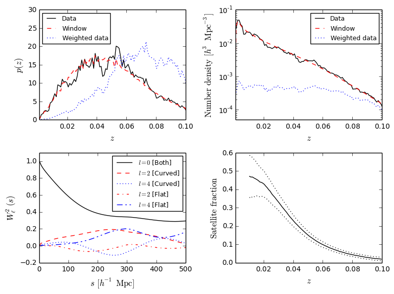
Figure 1: The upper left-hand and right-hand panels display, respectively, the redshift probability distribution and number density distribution averaged in redshift slices of the 6dFGS data sample (black solid line), the window function (red dashed line) and the data including the weights (blue dotted line). The lower left-hand panel plots the first three multipoles $W_{\ell}^{2}(s)$ of the window function in the range $s<500\,h^{-1}$ Mpc using curved-sky and flat-sky formulations, illustrating the importance of curved-sky effects for the $\ell>0$ terms. The lower right-hand panel illustrates the redshift dependence of the average satellite fraction in the mocks (with the standard deviation across mocks indicated by the dotted lines).

4 Application to the 6-degree Field Galaxy Survey

4.1 Data and mocks

The 6-degree Field Galaxy Survey (6dFGS, Jones et al., 2009; Springob et al., 2014) is a southern-hemisphere survey of $\sim 10^{5}$ galaxy redshifts and $\sim 10^{4}$ peculiar velocities carried out by the UK Schmidt Telescope between 2001 and 2006. Covering $17{,}000$ deg² of sky south of declination $0^{\circ}$ and located more than $10^{\circ}$ from the Galactic plane, and mapping galaxies with median redshift $0.053$, the 6dFGS remains one of the widest-angle studies of large-scale structure in the local Universe. The dataset has been subject to a number of previous cosmological analyses, including measurement and fitting of the baryon acoustic peak (Beutler et al., 2011), RSD fits to the 2D correlation function (Beutler et al., 2012), comparison studies of RSD around galaxies and voids (Achitouv et al., 2017), and analysis of the cross-correlation of peculiar velocities and densities (Adams & Blake, 2017). The growth rate of structure has also been measured using the statistics of the 6dFGS peculiar velocity field (Johnson et al., 2014; Huterer et al., 2017; Adams & Blake, 2017). As far as we are aware, there is no existing Fourier-space analysis of RSD using 6dFGS data.

In this Section we analyze the power spectrum multipoles of a subset of the 6dFGS redshift catalogue, forming a sample selected with magnitude $K<12.9$ in sky regions with redshift completeness greater than $60\%$, which is the sample used in the 6dFGS baryon acoustic peak study of Beutler et al. (2011). We restrict our analysis to galaxies in the redshift range $0.001<z<0.1$, given that the 6dFGS number density is very low at higher redshifts, producing a final sample of $70{,}467$ objects across $15{,}419$ deg². We map galaxies onto a 3D co-moving grid using a fiducial flat cosmological model with matter density $\Omega_{m}=0.3$ (matching the fiducial cosmology used to generate the mock catalogues, described below). When computing FFTs we enclose the hemispheric catalogue by a cuboid with dimensions $(586,586,293)\,h^{-1}$ Mpc and grid size $(128,128,64)$, such that the Nyquist sampling frequency in each dimension is $k_{\rm Nyq}\approx 0.7\,h$ Mpc^-1 (where we fit models to the range $k<0.2\,h$ Mpc^-1). We correct for this gridding effect in our power spectrum estimation.

We compute the window function $\langle n(\textbf{{x}})\rangle$ of the dataset following Jones et al. (2009) and Beutler et al. (2011), including the angular spectroscopic completeness and the variation of the redshift distribution with magnitude (hence local completeness). Galaxies are assigned an optimal weight depending on their position, combining the effects of sample variance and Poisson noise following Feldman et al. (1994):

$$w(\textbf{{x}})=\frac{1}{1+\langle n(\textbf{{x}})\rangle\,P_{0}},$$ (55)

where $P_{0}$ is a characteristic power spectrum amplitude. Following Beutler et al. (2012), we take $P_{0}=1{,}600\,h^{-3}$ Mpc³ (finding that our results are not overly sensitive to this choice). The upper panels of Figure 1 illustrate the redshift probability distribution and number density variation of the 6dFGS data and window function, including the effect of the weights assigned by Equation 55, which up-weight higher redshift (i.e., lower number density) data compared to lower redshift data, increasing the weighted mean redshift of the sample from $0.049$ to $0.067$. Defining the effective redshift of the power spectrum measurement as an optimally-weighted sum over the selection function,

$$z_{\rm eff}=\frac{\sum_{\textbf{{x}}}z\,W(\textbf{{x}})}{\sum_{\textbf{{x}}}W(\textbf{{x}})}$$ (56)

where $W(\textbf{{x}})=\left(\frac{\langle n(\textbf{{x}})\rangle P_{0}}{1+\langle n(\textbf{{x}})\rangle P_{0}}\right)^{2}$, we find $z_{\rm eff}=0.060$, which we take as the redshift of our growth rate measurement.

The lower left-hand panel of Figure 1 illustrates the first three window function multipoles $W_{\ell}^{2}(s)$, computed using the FFT-based method of Equation 27 in the range $s<500\,h^{-1}$ Mpc. These window function multipoles are used in Section 4.2 to test the convolution framework based on correlation function multipoles, compared to the purely Fourier-space method. We also determine the window function multipoles in the flat-sky approximation (i.e., using Equation 20 of Wilson et al. 2017). The evaluations are identical for $\ell=0$, but differ significantly for $\ell>0$, illustrating the importance of curved-sky effects for wide-area surveys.

We also use a set of $N_{\rm mock}=600$ mock catalogues produced as part of the 6dFGS baryon acoustic peak reconstruction analysis (Carter et al., 2018). These mock catalogues are generated by populating a set of dark matter halos produced by fast N-body techniques with a Halo Occupation Distribution of central and satellite galaxies, designed to match the redshift distribution and projected clustering of the 6dFGS sample; we refer the reader to Carter et al. (2018) for more details. The fiducial cosmological model used for the initial conditions of the mocks was $\Omega_{m}=0.3$, baryon density $\Omega_{b}=0.0478$, Hubble parameter $h=0.68$, clustering amplitude $\sigma_{8}=0.82$ and spectral index $n_{s}=0.96$. The fiducial normalized growth rate at $z=0$ is then $f\sigma_{8}=0.423$. We use the mocks to test the recovery of the input growth rate using our procedure, and to compare the Gaussian covariance with that deduced from the ensemble of mocks. The lower right-hand panel of Figure 1 displays the mean and standard deviation of the satellite fraction as a function of redshift across the 600 mocks; we will comment further on the effects of satellites in Section 4.3.

4.2 Power spectrum multipole models

For the purposes of this study we describe the dependence of the redshift-space galaxy power spectrum, $P(k,\mu)$, on the cosine of the angle to the line of sight, $\mu$, in terms of a simple 3-parameter model (Peacock & Dodds, 1994; Cole et al., 1995; Hatton & Cole, 1998) combining the large-scale Kaiser effect (Kaiser, 1987) imprinted by the growth rate $f$, exponential damping from random pairwise velocities with dispersion $\sigma_{v}$, and a linear galaxy bias $b$:

$$P(k,\mu)=\frac{(b+f\mu^{2})^{2}\,P_{m}(k)}{1+\left(k\mu\sigma_{v}/H_{0}\right)^{2}},$$ (57)

where $P_{m}(k)$ is the model matter power spectrum, which we compute using a recent version of the CAMB software package (Lewis et al., 2000), including the non-linear ‘halofit’ correction (Smith et al., 2003; Takahashi et al., 2012), for the fiducial cosmological parameters listed above. Given that $P_{m}(k)\propto\sigma_{8}^{2}$ on large scales, it is convenient for RSD analyses to adopt the parameter set $(f\sigma_{8},b\sigma_{8})$. The inclusion of the Hubble parameter $H_{0}=100\,h$ km s^-1 Mpc^-1 in Equation 57 implies that the pairwise velocity dispersion is measured in units of km s^-1 at $z=0$. The multipole power spectra may be computed from Equation 57 as

$$P_{\ell}(k)=\frac{2\ell+1}{2}\int_{-1}^{1}d\mu\,P(k,\mu)\,L_{\ell}(\mu).$$ (58)

Three multipoles $(\ell=0,2,4)$ are sufficient to describe the model in linear theory $(\sigma_{v}=0)$; in practice the hexadecapole contains extremely low signal-to-noise for current datasets such that analyses, including ours, focus on solely the monopole and quadrupole.

Many enhancements to the simple model of Equation 57 have been proposed, incorporating more accurate corrections for non-linear effects in the evolution of densities, velocities and galaxy bias (e.g., Scoccimarro, 2004; Taruya et al., 2010; Jennings et al., 2011; Reid & White, 2011). As we are focussing on testing the estimation, convolution and covariance of the clustering statistics, rather than performing the best possible measurement of the growth rate, the simple model of Equation 57 suits our purpose and we do not consider more sophisticated theoretical treatments.

Figure 2 illustrates the convolution of model power spectrum multipoles with the 6dFGS window function, computed using the two approaches described in Section 2.2 in bins of width $\Delta k=0.02\,h$ Mpc^-1 in the range $k<0.3\,h$ Mpc^-1. We use a fiducial parameter choice $f\sigma_{8}=0.423$, $\sigma_{v}=300$ km s^-1 and $b\sigma_{8}=1.19$, which is close to the best-fitting values for the 6dFGS data. We note the good agreement between the determination of the convolution using spherical harmonics and FFTs based on Equation 19, and the evaluation via the correlation function and window function multipoles, using Equations 22, 23 and 27. Small differences occur due to the sparse distribution of the grid of Fourier wavevectors k within each spherical shell in $k$-space. Figure 2 also verifies that the convolved quadrupole converges when Equation 19 is evaluated using the first two terms in $\ell^{\prime}$.

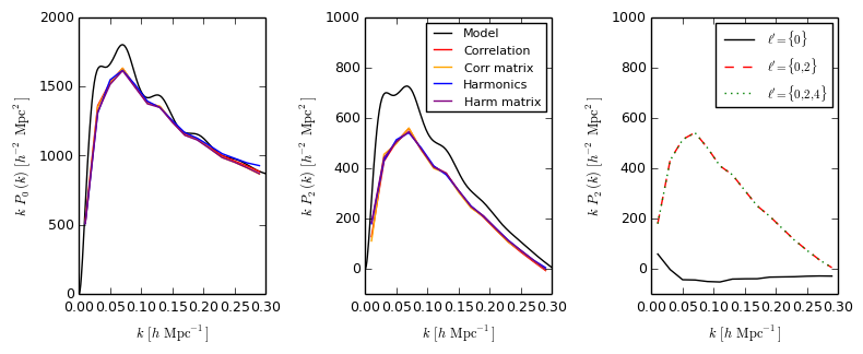
Figure 2: A consistency check of different determinations of the convolved monopole (left-hand panel) and quadrupole (middle panel) of a fiducial model (black line) with the survey window function, in a series of Fourier bins of width $\Delta k=0.02\,h$ Mpc^-1. Evaluations are shown using the correlation function and window function multipoles (red line), a convolution matrix derived by applying this method to a set of unit vectors as described in the text (orange line), the method using spherical harmonics and FFTs (blue line), and a corresponding convolution matrix (purple line). These different methods produce convolved power spectra in good agreement with each other. The right-hand panel displays a test of the number of multipoles $\ell^{\prime}$ in Equation 19 required for the evaluation of the convolved quadrupole to converge. We see that excellent convergence is obtained using 2 terms. The power spectra are scaled by a factor of $k$ for clarity of presentation.

Rather than re-compute a full convolution for each different RSD model, we determine a convolution matrix $M_{ij}$ in the Fourier bins $i$, such that the convolved multipole power spectrum $\hat{P}$, which is the concatenation of $(\hat{P}_{0},\hat{P}_{2},\hat{P}_{4})$, may be determined from the unconvolved power spectrum $P=(P_{0},P_{2},P_{4})$ as $\hat{P}_{i}=\sum_{j}M_{ij}\,P_{j}$. We evaluate the convolution matrix by applying the full convolution (Equation 19) to a set of unit model vectors $P_{j}$, generated such that $P_{\ell}(k)=1$ for the relevant multipole within a single bin $k_{{\rm min},j}<k<k_{{\rm max},j}$, and $P_{\ell}(k)=0$ for the remaining $k$-values and multipoles. We tested that this approach produced a negligible change in results compared to implementing the full convolution whilst being orders of magnitude faster to evaluate; these results are also displayed in Figure 2.

4.3 Power spectrum multipole measurements and errors

The monopole and quadrupole power spectra of the 6dFGS large-scale structure dataset, measured in 15 Fourier bins of width $\Delta k=0.02\,h$ Mpc^-1 in the range $k<0.3\,h$ Mpc^-1, are displayed in Figure 3 together with the best-fitting model. We postpone a discussion of the best-fitting model parameters to the next section, and focus here on the errors in the measured statistics. We note the upward sample variance fluctuation in the monopole at the scale corresponding to the baryon acoustic peak ($k\approx 0.07\,h$ Mpc^-1), which may contribute toward the strong signature of the acoustic peak in the 6dFGS correlation function reported by Beutler et al. (2011), which was found by that study to lie in the upper quartile of statistical realizations. The hexadecapole power spectrum does not contain any useful signal and we do not consider it further.

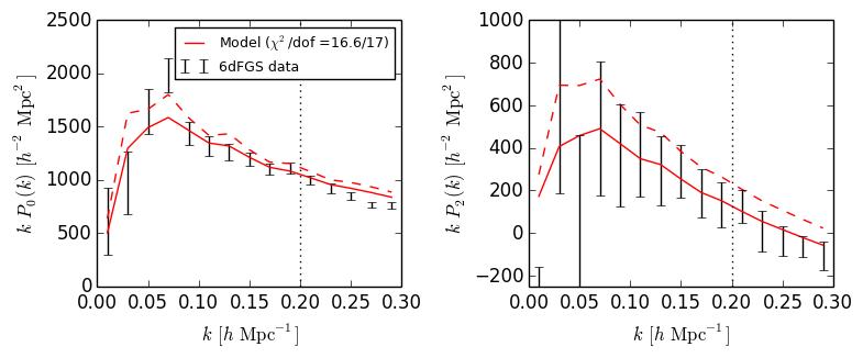
Figure 3: The monopole (left-hand panel) and quadrupole (right-hand panel) power spectra of the $z<0.1$ 6dFGS $K$-band galaxy sample, applying FKP weighting with characteristic amplitude $P_{0}=1{,}600\,h^{-3}$ Mpc³. The dashed and solid lines show, respectively, the unconvolved and convolved best-fitting 3-parameter RSD model fit to the monopole and quadrupole in the wavenumber range $k<0.2\,h$ Mpc^-1 (indicated by the vertical dotted lines), with the corresponding $\chi^{2}$ value indicated in the plot. Convolution with a window function reduces the amplitude of a model power spectrum model, because a selection function always contains a smaller effective volume than the cube in which it is embedded, such that the convolved power is carried by a higher number density of Fourier modes (Peacock & Nicholson, 1991). The errors are determined using the Gaussian approximation to the covariance matrix, generated from this best-fitting model. The power spectra are scaled by a factor of $k$ for clarity of presentation.

Figure 4 compares the standard deviation of the monopole and quadrupole power spectrum (i.e., the square root of the diagonal values of the covariance matrix, $\sqrt{C_{ii}}$) for the 6dFGS data and mocks, estimated using different techniques. These determinations use either the Gaussian covariance of Section 3, or are estimated from the ensemble of mock catalogues as

$$C_{ij}=\frac{1}{N_{\rm mock}-1}\left[\sum_{k}\left(P_{i,k}-\overline{P_{i}}\right)\left(P_{j,k}-\overline{P_{j}}\right)\right]=\frac{N_{\rm mock}}{N_{\rm mock}-1}\left(\overline{P_{i}P_{j}}-\overline{P_{i}}\;\overline{P_{j}}\right),$$ (59)

where $P_{i}$ is the concatenation of the monopole and quadrupole in a combined data vector of 30 entries, $P_{i,k}$ is the measurement of these values in the $k$-th mock, and $\overline{P_{i}}=(1/N_{\rm mock})\sum_{k=1}^{N_{\rm mock}}P_{i,k}$ is the average value across the ensemble of mocks. The Gaussian covariance evaluation uses the window function $\langle n(\textbf{{x}})\rangle$ and requires a choice of fiducial multipole power spectra for each sample. We compute the fiducial power spectra from Equation 57 with $f\sigma_{8}=0.423$, $\sigma_{v}=300$ km s^-1 and $b\sigma_{8}=(1.19,1.04,0.84)$ for the data, mocks including satellites and mocks excluding satellites, respectively, which are close to the best-fitting values in each case. The inclusion of satellites in the mock increases the fiducial bias factor.

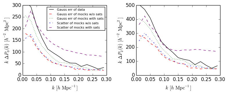
Figure 4: Comparison of the errors in the monopole (left-hand panel) and quadrupole (right-hand panel) power spectra of the 6dFGS data sample and corresponding mock catalogues, including and excluding satellites. The different error determinations apply either the Gaussian approximation to the covariance, or measure the standard deviation of the power spectrum multipole estimates across the mock catalogues. The inclusion of satellites increases the standard deviation of the mock power spectra above the Gaussian estimate; the amplitude variation in the Gaussian covariance determinations at low $k$ is driven by the different fiducial bias factors in each case. The power spectra are scaled by a factor of $k$ for clarity of presentation.

It is interesting to compare mock catalogues including and excluding satellite galaxies. The inclusion of satellites, which are located preferentially in high-mass halos, enhances the clustering power by up-weighting massive halos, and causes the Poisson sampling model described by Equation 10 to break down (Baldauf et al., 2013; Ginzburg et al., 2017). For central-only galaxy samples, the Gaussian error agrees well with the dispersion across the mock catalogues, as illustrated by the comparison of the red and blue lines in Figure 4. The inclusion of satellites complicates the picture, increasing the standard deviation of the mock power spectra above the Gaussian estimate. Since the sample variance contribution to the covariance scales as $(b\sigma_{8})^{2}$ on large scales, the different fiducial bias values drive the amplitude variations in the Gaussian covariance at low $k$.

Figure 5 provides further insight by illustrating the correlation matrix, which quantifies the amplitude of the off-diagonal covariance compared to the diagonal elements as $C_{ij}/\sqrt{C_{ii}\,C_{jj}}$, corresponding to various cases. The left-hand panel displays the covariance of the 6dFGS data in the Gaussian approximation, evaluated using the methodology of Section 3. The central panel is the covariance evaluated across the ensemble of mock catalogues, excluding satellites. The correlation structure of the principal diagonals and first off-diagonal of the two matrices is similar. The mock-based matrix contains somewhat greater correlation than the Gaussian approximation between bins that are widely separated in $k$, typically with a cross-correlation coefficient less than $0.2$, but at a somewhat higher level for monopole covariance at $k>0.2\,h$ Mpc^-1 (noting that we do not fit to these scales). The right-hand panel displays the mock covariance including satellite galaxies, featuring a significant enhancement in the off-diagonal covariance with increasing $k$. Evidently, satellites in the 6dFGS HOD mock (which constitute a significant fraction of the sample, as illustrated by Figure 1) have a strong impact in correlating different scales of the power spectrum monopole and quadrupole, and anti-correlating the monopole and quadrupole. This effect may arise because the trispectrum component, which drives significant off-diagonal covariance in Fourier space (Howlett & Percival, 2017), is boosted by the significant satellite fraction in these mocks, and the effect is extended across a wide range of scales by the significant width of the $k$-space window function of this small-volume survey. In the next Section we will explore the impact of these differences on the RSD parameter fits for the 6dFGS data and mocks.

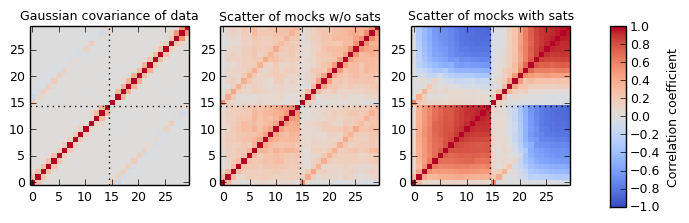
Figure 5: The correlation matrix of the monopole and quadrupole, derived from the covariance matrix $C_{ij}$ as $C_{ij}/\sqrt{C_{ii}\,C_{jj}}$. The 30 bins correspond to the concatenation $(P_{0},P_{2})$ for measurements up to $k=0.3\,h$ Mpc^-1 in bins of width $\Delta k=0.02\,h$ Mpc^-1. Three cases are shown, from left-to-right: the 6dFGS data sample covariance determined in the Gaussian approximation, and the covariance deduced from the ensemble of mock catalogues excluding satellites and including satellites.

4.4 RSD parameter fits

We fit the RSD power spectrum model of Equation 57 to the monopole and quadrupole of the 6dFGS data and mocks over the range $k<0.2\,h$ Mpc^-1, varying the 3 parameters $(f\sigma_{8},\sigma_{v},b\sigma_{8})$. We first consider the results of fitting to the mock catalogues, both excluding and including satellites. The mean power spectrum monopole and quadrupole, averaged across the 600 mocks, is displayed in the upper panels of Figure 6, with the error (as appropriate for a single mock) computed using the Gaussian approximation to the covariance. The increased low-$k$ errors in the power spectra for the mocks with satellites is driven by the increased effective galaxy bias factor, recalling that the sample variance contribution to the covariance scales as $(b\sigma_{8})^{2}$ on large scales. We overplot the best-fitting RSD models, which provide a good description of the measurements over the fitted range.

Figure 6: The power spectrum multipole measurements and RSD parameter fits obtained from the 6dFGS mock catalogues, considering cases excluding and including satellites (displayed in blue and red, respectively, and offset along the $x$-axis for clarity). The upper-left and upper-right panels display the mock mean monopole and quadrupole power spectra, with errors determined using the Gaussian approximation to the covariance. The solid lines in these panels are the best-fitting models in each case, with the vertical dotted line indicating the maximum fitted scale ($k=0.2\,h$ Mpc^-1). The lower-left panel shows the $68\%$ confidence region of the 2D posterior probability distribution for the normalized growth rate $f\sigma_{8}$ and velocity dispersion $\sigma_{v}$, marginalized over the galaxy bias $b\sigma_{8}$, and the right-hand panel shows the marginalized probability distribution for the growth rate. The growth rate ranges quoted in the right-hand panel are $68\%$ confidence intervals. The vertical dotted line in the lower panels indicates the growth rate expected in the fiducial $\Omega_{m}=0.3$ model. The inclusion of satellites causes a systematic shift in the best-fitting growth rate, owing to the breakdown of the exponential damping model. However, this shift is smaller than the statistical error in the measurement.

The lower panels of Figure 6 illustrate the posterior probabilities of the RSD parameters. The marginalized measurements of the normalized growth rate are $f\sigma_{8}=(0.45\pm 0.09)$ and $(0.32\pm 0.10)$ for the sample excluding and including satellites, respectively, compared to the fiducial value of $0.42$. Satellites create systematic error in the model of Equation 57, where a simple exponential damping scenario is unable to represent their effect in detail. We conclude that, at the level of precision afforded by the 6dFGS sample, the model of Equation 57 provides an acceptable description of the clustering pattern over the range $k<0.2\,h$ Mpc^-1, although it would suffer from systematic modelling errors given significantly larger datasets, especially due to the presence of satellites. For comparison, we note that an RSD fit to $k<0.1\,h$ Mpc^-1 produces marginalized measurements $f\sigma_{8}=(0.43\pm 0.11)$ and $(0.37\pm 0.13)$ excluding and including satellites, in closer agreement with the fiducial value of $0.42$, and a fit to $k<0.3\,h$ Mpc^-1 produces fits with significantly enhanced systematic errors, respectively $f\sigma_{8}=(0.50\pm 0.06)$ and $(0.31\pm 0.06)$.

We now consider the corresponding RSD parameter fits to the 6dFGS data sample, also using the fitting range $k<0.2\,h$ Mpc^-1. The best-fitting unconvolved and convolved models using the Gaussian covariance are overplotted in Figure 3, and Figure 7 displays the $68\%$ confidence region of the joint posterior probability distribution for $(f\sigma_{8},\sigma_{v})$ (left-hand panel), and the marginalized probability distribution for the normalized growth rate (right-hand panel). We consider various cases. Our fiducial analysis, using our new convolution treatment described in Section 2.2 and the Gaussian covariance matrix, produces marginalized parameter fits $f\sigma_{8}=0.38\pm 0.12$, $\sigma_{v}=290\pm 120$ km s^-1 and $b\sigma_{8}=1.19\pm 0.03$ (quoting $68\%$ confidence regions), with minimum $\chi^{2}=16.6$ for 17 degrees-of-freedom. Replacing the convolution scheme with a method using window function and correlation function multipoles produces almost identical results. Using the covariance matrix deduced from mock catalogues including satellites produces consistent best-fitting parameters (the growth rate fit is $f\sigma_{8}=0.36\pm 0.13$), but the minimum $\chi^{2}$ increases to $34.3$, driven by the off-diagonal terms of the covariance matrix shown in Figure 5.

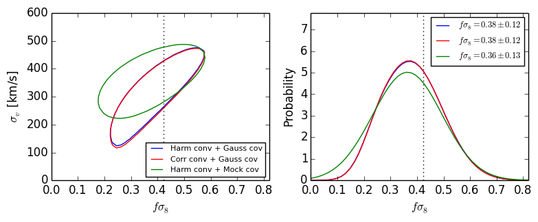
Figure 7: RSD parameter fits to the 6dFGS galaxy sample. The left-hand panel displays the $68\%$ confidence region of the 2D posterior probability distribution for the normalized growth rate $f\sigma_{8}$ and velocity dispersion $\sigma_{v}$, marginalized over the galaxy bias $b\sigma_{8}$, and the right-hand panel shows the marginalized probability distribution for the growth rate. Results are displayed for three cases: using spherical harmonics convolution and the covariance matrix derived using the Gaussian approximation (‘Harm conv + Gauss cov’, blue contours); correlation function convolution with the same covariance (‘Corr conv + Gauss cov’, red contours) and spherical harmonics convolution with the covariance matrix derived from mock catalogues (‘Harm conv + Mock cov’, green contours). The growth rate ranges quoted in the right-hand panel are $68\%$ confidence intervals. The vertical dotted line indicates the growth rate expected in a fiducial $\Omega_{m}=0.3$ model. The analyses using different convolution and covariance approaches produce consistent results.

Our growth rate fitted to the 6dFGS power spectrum multipoles agrees well with previous analyses of the 6dFGS redshift and peculiar velocity samples. Beutler et al. (2012) and Achitouv et al. (2017) both report a measurement $f\sigma_{8}=0.42\pm 0.06$ obtained by fitting RSD models to the 2D galaxy correlation function, and similar results are obtained when fitting to the 2-point clustering of peculiar velocities and density-velocity correlations (Johnson et al., 2014; Huterer et al., 2017; Adams & Blake, 2017). The error in our measured growth rate is roughly a factor of 2 higher than these correlation function studies. We compared our fitted error in the growth rate to that forecast by a standard Fisher matrix calculation (e.g., White et al., 2009; Abramo, 2012; Blake et al., 2013). Assuming an idealized survey with the area and redshift distribution of our 6dFGS sample and neglecting covariance between Fourier modes, we forecast an error $\sigma(f\,\sigma_{8})=0.10$ for a fit to the wavenumber range $k<0.2\,h$ Mpc^-1. The error in our measurement is only $20\%$ larger than this forecast, suggesting that it is realistic and that the correlation function fits are accessing information on smaller scales. Improved Fourier-space modelling would be required to extend the power spectrum fits to these scales.

5 Summary

The correlated peculiar velocities of galaxies, generated by the gravitational physics of the clustered density field, modulate redshift-space galaxy clustering with respect to the local line of sight. These directional anisotropies may be described in terms of a multipole expansion of the clustering pattern. The changing line-of-sight direction across a galaxy survey complicates the analysis of clustering multipoles, particularly in Fourier space, where the survey volume is embedded within an enclosing cuboid to allow the application of efficient FFT techniques.

In this study we have explored three extensions of power spectrum multipole calculations. First, we derived an alternative formulation of the convolution of the power spectrum multipoles with a survey window function in a curved sky, in the local plane-parallel approximation. This expression is evaluated purely in Fourier space using FFTs, and produces very similar results to approaches using the correlation function and window function multipoles, whilst avoiding the need for mapping the statistics into configuration space. Second, we developed expressions for the joint covariance of power spectrum multipoles within a Gaussian approximation, including window function and curved-sky effects. Finally, we generalized these results to include the cross-power spectrum multipoles of overlapping galaxy tracers. Accompanying python code is available at https://github.com/cblakeastro/multipoles.

We applied our framework to conduct the first Fourier-space clustering analysis of the 6-degree Field Galaxy Survey. By fitting a simple RSD model to the monopole and quadrupole in the range $k<0.2\,h$ Mpc^-1, we determined a best-fitting growth rate $f\sigma_{8}=0.38\pm 0.12$ at effective redshift $z=0.06$, in agreement with previous 6dFGS analyses. The statistical error of our measurement agrees with a Fisher matrix error forecast, although is twice as large as previous correlation function analyses, which access smaller scales. We verified our fitting pipeline using a series of mock catalogues, demonstrating the impact of satellite galaxies on covariance properties. We note that techniques such as cylindrical exclusion (Okumura et al., 2017) can reduce the impact of satellites on clustering analyses.

Future galaxy redshift surveys such as the Taipan Galaxy Survey (da Cunha et al., 2017), the Dark Energy Spectroscopic Instrument (DESI Collaboration et al., 2016) and the 4MOST Cosmology Redshift Survey (de Jong et al., 2012) will allow the clustering of the local and distant Universe to be quantified with increasing accuracy, and cosmological models to be precisely tested. Power spectrum multipoles will continue to provide a valuable connection between observations and theory.

Appendix A Derivation of convolution using correlation function multipoles

For completeness we derive in this Appendix the evaluation of Equation 11 using a multipole expansion of the correlation function (Wilson et al., 2017; Beutler et al., 2017), $\xi(\textbf{{x}},\textbf{{x}}^{\prime})=\sum_{\ell^{\prime}}\xi_{\ell^{\prime}}(s)\,L_{\ell^{\prime}}(\hat{\textbf{{s}}}.\hat{\textbf{{x}}}^{\prime})$ where $\textbf{{s}}=\textbf{{x}}^{\prime}-\textbf{{x}}$, such that

$$\langle\hat{P}_{\ell}(k)\rangle=\frac{2\ell+1}{I}\int\frac{d\Omega_{k}}{4\pi}\,\frac{1}{V}\int d^{3}\textbf{{x}}\,n_{w}(\textbf{{x}})\int d^{3}\textbf{{s}}\,n_{w}(\textbf{{x}}+\textbf{{s}})\,e^{i\textbf{{k}}.\textbf{{s}}}\,L_{\ell}(\hat{\textbf{{k}}}.\hat{\textbf{{x}}})\sum_{\ell^{\prime}}\xi_{\ell^{\prime}}(s)\,L_{\ell^{\prime}}(\hat{\textbf{{s}}}.\hat{\textbf{{x}}}).$$ (60)

We note that the model correlation function multipoles $\xi_{\ell}$ may be determined from the power spectrum multipoles using the inverse transform of Equation 22:

$$\xi_{\ell}(s)=\frac{(-i)^{\ell}}{2\pi^{2}}\int dk\,k^{2}\,j_{\ell}(ks)\,P_{\ell}(k).$$ (61)

Using the plane wave expansion of Equation 26 we obtain

$$\langle\hat{P}_{\ell}(k)\rangle=\frac{2\ell+1}{I}\frac{1}{V}\int d^{3}\textbf{{x}}\,n_{w}(\textbf{{x}})\int d^{3}\textbf{{s}}\,n_{w}(\textbf{{x}}+\textbf{{s}})\sum_{\ell^{\prime}}\xi_{\ell^{\prime}}(s)\,L_{\ell^{\prime}}(\hat{\textbf{{s}}}.\hat{\textbf{{x}}})\sum_{\ell^{\prime\prime}}i^{\ell^{\prime\prime}}\,(2\ell^{\prime\prime}+1)\,j_{\ell^{\prime\prime}}(ks)\int\frac{d\Omega_{k}}{4\pi}\,L_{\ell}(\hat{\textbf{{k}}}.\hat{\textbf{{x}}})\,L_{\ell^{\prime\prime}}(\hat{\textbf{{k}}}.\hat{\textbf{{s}}}).$$ (62)

Using the result $\int\frac{d\Omega_{k}}{4\pi}\,L_{\ell}(\hat{\textbf{{k}}}.\hat{\textbf{{x}}})\,L_{\ell^{\prime}}(\hat{\textbf{{k}}}.\hat{\textbf{{s}}})=\frac{1}{2\ell+1}\,L_{\ell}(\hat{\textbf{{s}}}.\hat{\textbf{{x}}})\,\delta_{\ell,\ell^{\prime}}$, we can simplify this expression to the form

$$\langle\hat{P}_{\ell}(k)\rangle=\frac{2\ell+1}{I}\frac{1}{V}\int d^{3}\textbf{{x}}\,n_{w}(\textbf{{x}})\int d^{3}\textbf{{s}}\,n_{w}(\textbf{{x}}+\textbf{{s}})\sum_{\ell^{\prime}}\xi_{\ell^{\prime}}(s)\,L_{\ell^{\prime}}(\hat{\textbf{{s}}}.\hat{\textbf{{x}}})\,i^{\ell}\,j_{\ell}(ks)\,L_{\ell}(\hat{\textbf{{s}}}.\hat{\textbf{{x}}}).$$ (63)

It is convenient to write this relation in the form of an inverse transform to Equation 61,

$$\langle\hat{P}_{\ell}(k)\rangle=4\pi\,i^{\ell}\int ds\,s^{2}\,j_{\ell}(ks)\,\hat{\xi}_{\ell}(s),$$ (64)

where

$$\hat{\xi}_{\ell}(s)=\frac{2\ell+1}{I}\,\frac{1}{V}\int d^{3}\textbf{{x}}\,n_{w}(\textbf{{x}})\int\frac{d\Omega_{s}}{4\pi}\,n_{w}(\textbf{{x}}+\textbf{{s}})\sum_{\ell^{\prime}}\xi_{\ell^{\prime}}(s)\,L_{\ell}(\hat{\textbf{{s}}}.\hat{\textbf{{x}}})\,L_{\ell^{\prime}}(\hat{\textbf{{s}}}.\hat{\textbf{{x}}}).$$ (65)

We can conveniently evaluate this expression using the Legendre expansion of a product of Legendre polynomials (Adams, 1878):

$$L_{\ell}(x)\,L_{\ell^{\prime}}(x)=\sum_{\ell^{\prime\prime}=|\ell-\ell^{\prime}|}^{\ell+\ell^{\prime}}\left(\begin{matrix}\ell&\ell^{\prime}&\ell^{\prime\prime}\\ 0&0&0\end{matrix}\right)^{2}\,(2\ell^{\prime\prime}+1)\,L_{\ell^{\prime\prime}}(x)=\sum_{\ell^{\prime\prime}}A^{\ell^{\prime\prime}}_{\ell,\ell^{\prime}}\,L_{\ell^{\prime\prime}}(x),$$ (66)

where $\left(\begin{matrix}\ell&\ell^{\prime}&\ell^{\prime\prime}\\ 0&0&0\end{matrix}\right)$ is a Wigner 3j-symbol, and the coefficients $A^{\ell^{\prime\prime}}_{\ell,\ell^{\prime}}$ are given by Bailey (1933) as

$$A^{\ell^{\prime\prime}}_{\ell,\ell^{\prime}}=\left(\begin{matrix}\ell&\ell^{\prime}&\ell^{\prime\prime}\\ 0&0&0\end{matrix}\right)^{2}\,(2\ell^{\prime\prime}+1)=\frac{G_{\ell-p}\,G_{p}\,G_{\ell^{\prime}-p}}{G_{\ell+\ell^{\prime}-p}}\left(\frac{2\ell+2\ell^{\prime}-4p+1}{2\ell+2\ell^{\prime}-2p+1}\right),$$ (67)

in which $G_{p}=[1.3...(2p-1)]/[p!]$, $\ell^{\prime\prime}=\ell+\ell^{\prime}-2p$ and, in the sum over $\ell^{\prime\prime}$ defined by Equation 66, $p$ ranges from $0$ to ${\rm min}(\ell,\ell^{\prime})$. Using this notation we can write

$$\hat{\xi}_{\ell}(s)=(2\ell+1)\sum_{\ell^{\prime}}\xi_{\ell^{\prime}}(s)\sum_{\ell^{\prime\prime}}A^{\ell^{\prime\prime}}_{\ell,\ell^{\prime}}\,\frac{W_{\ell^{\prime\prime}}^{2}(s)}{2\ell^{\prime\prime}+1},$$ (68)

in terms of the window function multipoles

$$W_{\ell}^{2}(s)=\frac{2\ell+1}{I}\int\frac{d\Omega_{s}}{4\pi}\,\frac{1}{V}\int d^{3}\textbf{{x}}\,n_{w}(\textbf{{x}})\,n_{w}(\textbf{{x}}+\textbf{{s}})\,L_{\ell}(\hat{\textbf{{x}}}.\hat{\textbf{{s}}}),$$ (69)

in agreement with Equation A9 of Beutler et al. (2017). For example

$$\hat{\xi}_{0}(s)=W_{0}^{2}(s)\,\xi_{0}(s)+\frac{1}{5}\,W_{2}^{2}(s)\,\xi_{2}(s)+\frac{1}{9}\,W_{4}^{2}(s)\,\xi_{4}(s)+...$$ (70)

since if $\ell=0$, then $p=0$ and $A^{\ell^{\prime}}_{0,\ell^{\prime}}=1$. Relations for the other “convolved” multipoles $\hat{\xi}_{\ell}$, in terms of $\xi_{\ell}$, are provided by Wilson et al. (2017) and Beutler et al. (2017).

We can use Equation 27 to check a couple of useful special cases. First,

$$W_{0}^{2}(0)=\frac{1}{I}\frac{V}{(2\pi)^{3}}\int d^{3}\textbf{{k}}\,|\tilde{n}_{w}(\textbf{{k}})|^{2}=\frac{1}{I}\,\frac{1}{V}\int d^{3}\textbf{{x}}\,n_{w}^{2}(\textbf{{x}})=1.$$ (71)

Also, for a constant window function $n(\textbf{{x}})=n_{0}$ we find

$$W_{\ell}^{2}(s)=\frac{4\pi\,i^{\ell}}{n_{0}^{2}}\sum_{m=-\ell}^{\ell}\,n_{0}\,j_{\ell}(0)\,Y_{\ell,m}(\hat{\textbf{{0}}})\,\frac{1}{V}\int d^{3}\textbf{{x}}\,n_{0}\,Y_{\ell,m}^{*}(\hat{\textbf{{x}}})=\delta_{\ell,0},$$ (72)

where $\delta_{\ell,0}$ is a Kronecker delta.

References

- Abramo (2012) Abramo L. R., 2012, MNRAS, 420, 2042
- Achitouv et al. (2017) Achitouv I., Blake C., Carter P., Koda J., Beutler F., 2017, Phys. Rev. D, 95, 083502
- Adams (1878) Adams J., 1878, Proceedings of the Royal Society of London, 27, 63
- Adams & Blake (2017) Adams C., Blake C., 2017, MNRAS, 471, 839
- Alam et al. (2017) Alam S., et al., 2017, MNRAS, 470, 2617
- Astropy Collaboration et al. (2013) Astropy Collaboration et al., 2013, A&A, 558, A33
- Bailey (1933) Bailey W. N., 1933, Mathematical Proceedings of the Cambridge Philosophical Society, 29, 173
- Baldauf et al. (2013) Baldauf T., Seljak U., Smith R. E., Hamaus N., Desjacques V., 2013, Phys. Rev. D, 88, 083507
- Beutler et al. (2011) Beutler F., et al., 2011, MNRAS, 416, 3017
- Beutler et al. (2012) Beutler F., et al., 2012, MNRAS, 423, 3430
- Beutler et al. (2014) Beutler F., et al., 2014, MNRAS, 443, 1065
- Beutler et al. (2017) Beutler F., et al., 2017, MNRAS, 466, 2242
- Bianchi et al. (2015) Bianchi D., Gil-Marín H., Ruggeri R., Percival W. J., 2015, MNRAS, 453, L11
- Blake et al. (2011) Blake C., et al., 2011, MNRAS, 415, 2876
- Blake et al. (2013) Blake C., et al., 2013, MNRAS, 436, 3089
- Carter et al. (2018) Carter P., Beutler F., Percival W. J., Blake C., Koda J., Ross A. J., 2018, preprint, (arXiv:1803.01746)
- Castorina & White (2018) Castorina E., White M., 2018, MNRAS, 476, 4403
- Cole et al. (1994) Cole S., Fisher K. B., Weinberg D. H., 1994, MNRAS, 267, 785
- Cole et al. (1995) Cole S., Fisher K. B., Weinberg D. H., 1995, MNRAS, 275, 515
- DESI Collaboration et al. (2016) DESI Collaboration et al., 2016, preprint, (arXiv:1611.00036)
- Feldman et al. (1994) Feldman H. A., Kaiser N., Peacock J. A., 1994, ApJ, 426, 23
- Gil-Marín et al. (2010) Gil-Marín H., Wagner C., Verde L., Jimenez R., Heavens A. F., 2010, MNRAS, 407, 772
- Gil-Marín et al. (2016) Gil-Marín H., et al., 2016, MNRAS, 460, 4188
- Ginzburg et al. (2017) Ginzburg D., Desjacques V., Chan K. C., 2017, Phys. Rev. D, 96, 083528
- Grieb et al. (2016) Grieb J. N., Sánchez A. G., Salazar-Albornoz S., Dalla Vecchia C., 2016, MNRAS, 457, 1577
- Hamilton (1998) Hamilton A. J. S., 1998, in Hamilton D., ed., Astrophysics and Space Science Library Vol. 231, The Evolving Universe. p. 185 (arXiv:astro-ph/9708102), doi:10.1007/978-94-011-4960-0_17
- Hamilton (2000) Hamilton A. J. S., 2000, MNRAS, 312, 257
- Hand et al. (2017) Hand N., Li Y., Slepian Z., Seljak U., 2017, J. Cosmology Astropart. Phys., 7, 002
- Hartlap et al. (2007) Hartlap J., Simon P., Schneider P., 2007, A&A, 464, 399
- Hatton & Cole (1998) Hatton S., Cole S., 1998, MNRAS, 296, 10
- Howlett & Percival (2017) Howlett C., Percival W. J., 2017, MNRAS, 472, 4935
- Howlett et al. (2015) Howlett C., Ross A. J., Samushia L., Percival W. J., Manera M., 2015, MNRAS, 449, 848
- Huchra et al. (2012) Huchra J. P., et al., 2012, ApJS, 199, 26
- Hunter (2007) Hunter J. D., 2007, Computing In Science & Engineering, 9, 90
- Huterer et al. (2017) Huterer D., Shafer D. L., Scolnic D. M., Schmidt F., 2017, J. Cosmology Astropart. Phys., 5, 015
- Jennings et al. (2011) Jennings E., Baugh C. M., Pascoli S., 2011, MNRAS, 410, 2081
- Johnson et al. (2014) Johnson A., et al., 2014, MNRAS, 444, 3926
- Jones et al. (2009) Jones D. H., et al., 2009, MNRAS, 399, 683
- Kaiser (1987) Kaiser N., 1987, MNRAS, 227, 1
- Lewis et al. (2000) Lewis A., Challinor A., Lasenby A., 2000, ApJ, 538, 473
- McDonald & Seljak (2009) McDonald P., Seljak U., 2009, J. Cosmology Astropart. Phys., 10, 007
- Mohammed et al. (2017) Mohammed I., Seljak U., Vlah Z., 2017, MNRAS, 466, 780
- O’Connell et al. (2016) O’Connell R., Eisenstein D., Vargas M., Ho S., Padmanabhan N., 2016, MNRAS, 462, 2681
- Okumura et al. (2017) Okumura T., Takada M., More S., Masaki S., 2017, MNRAS, 469, 459
- Pápai & Szapudi (2008) Pápai P., Szapudi I., 2008, MNRAS, 389, 292
- Peacock & Dodds (1994) Peacock J. A., Dodds S. J., 1994, MNRAS, 267, 1020
- Peacock & Nicholson (1991) Peacock J. A., Nicholson D., 1991, MNRAS, 253, 307
- Pezzotta et al. (2017) Pezzotta A., et al., 2017, A&A, 604, A33
- Reid & White (2011) Reid B. A., White M., 2011, MNRAS, 417, 1913
- Samushia et al. (2012) Samushia L., Percival W. J., Raccanelli A., 2012, MNRAS, 420, 2102
- Scoccimarro (2004) Scoccimarro R., 2004, Phys. Rev. D, 70, 083007
- Scoccimarro (2015) Scoccimarro R., 2015, Phys. Rev. D, 92, 083532
- Seljak et al. (2009) Seljak U., Hamaus N., Desjacques V., 2009, Physical Review Letters, 103, 091303
- Slepian & Eisenstein (2015a) Slepian Z., Eisenstein D. J., 2015a, preprint, (arXiv:1510.04809)
- Slepian & Eisenstein (2015b) Slepian Z., Eisenstein D. J., 2015b, MNRAS, 454, 4142
- Slepian & Eisenstein (2016) Slepian Z., Eisenstein D. J., 2016, MNRAS, 455, L31
- Smith (2009) Smith R. E., 2009, MNRAS, 400, 851
- Smith et al. (2003) Smith R. E., et al., 2003, MNRAS, 341, 1311
- Springob et al. (2014) Springob C. M., et al., 2014, MNRAS, 445, 2677
- Sugiyama et al. (2018) Sugiyama N. S., Shiraishi M., Okumura T., 2018, MNRAS, 473, 2737
- Takahashi et al. (2012) Takahashi R., Sato M., Nishimichi T., Taruya A., Oguri M., 2012, ApJ, 761, 152
- Taruya et al. (2010) Taruya A., Nishimichi T., Saito S., 2010, Phys. Rev. D, 82, 063522
- Taylor & Joachimi (2014) Taylor A., Joachimi B., 2014, MNRAS, 442, 2728
- White et al. (2009) White M., Song Y.-S., Percival W. J., 2009, MNRAS, 397, 1348
- Wilson et al. (2017) Wilson M. J., Peacock J. A., Taylor A. N., de la Torre S., 2017, MNRAS, 464, 3121
- Xu et al. (2012) Xu X., Padmanabhan N., Eisenstein D. J., Mehta K. T., Cuesta A. J., 2012, MNRAS, 427, 2146
- Yamamoto et al. (2006) Yamamoto K., Nakamichi M., Kamino A., Bassett B. A., Nishioka H., 2006, PASJ, 58, 93
- Yoo & Seljak (2015) Yoo J., Seljak U., 2015, MNRAS, 447, 1789
- da Cunha et al. (2017) da Cunha E., et al., 2017, Publ. Astron. Soc. Australia, 34, e047
- de Jong et al. (2012) de Jong R. S., et al., 2012, in Ground-based and Airborne Instrumentation for Astronomy IV. p. 84460T (arXiv:1206.6885), doi:10.1117/12.926239