BlueTides simulation: establishing black hole-galaxy relations at high-redshift

Abstract

The scaling relations between the mass of supermassive black holes ($M_{\bullet}$) and host galaxy properties (stellar mass, $M_{\star}$, and velocity dispersion, $\sigma$), provide a link between the growth of black holes (BHs) and that of their hosts. Here we investigate if and how the BH-galaxy relations are established in the high-$z$ universe using BlueTides, a high-resolution large volume cosmological hydrodynamic simulation. We find the $M_{\bullet}-M_{\star}$ and $M_{\bullet}-\sigma$ relations at $z=8$: $\log_{10}(M_{\bullet})=8.25+1.10\ \log_{10}(M_{\star}/10^{11}M_{\sun})$ and $\log_{10}(M_{\bullet})=8.35+5.31\ \log_{10}(\sigma/200kms^{-1})$ at $z=8$, both fully consistent with the local measurements. The slope of the $M_{\bullet}-\sigma$ relation is slightly steeper for high star formation rate and $M_{\star}$ galaxies while it remains unchanged as a function of Eddington accretion rate onto the BH. The intrinsic scatter in $M_{\bullet}-\sigma$ relation in all cases ($\epsilon\sim 0.4$) is larger at these redshifts than inferred from observations and larger than in $M_{\bullet}-M_{\star}$ relation ($\epsilon\sim 0.14$). We find the gas-to-stellar ratio $f=M_{\rm gas}/M_{\star}$ in the host (which can be very high at these redshifts) to have the most significant impact setting the intrinsic scatter of $M_{\bullet}-\sigma$. The scatter is significantly reduced when galaxies with high gas fractions ($\epsilon=0.28$ as $f<10$) are excluded (making the sample more comparable to low-$z$ galaxies); these systems have the largest star formation rates and black hole accretion rates, indicating that these fast-growing systems are still moving toward the relation at these high redshifts. Examining the evolution (from $z=10$ to 8) of high mass black holes in $M_{\bullet}-\sigma$ plane confirms this trend.

1 Introduction

Over the last three decades, scaling relations between mass of supermassive black holes (SMBHs) and several stellar properties of their host galaxies such as bulge stellar mass and bulge velocity dispersion (Magorrian et al., 1998; Häring & Rix, 2004; Gebhardt et al., 2000; Tremaine et al., 2002; Gültekin et al., 2009; Kormendy & Ho, 2013; McConnell & Ma, 2013; Reines & Volonteri, 2015) have been discovered and measured for galaxies with black holes (BHs) and active galactic nuclei (AGN) from $z=0$ and up to $z\sim 2$ (using different techniques).

Many theoretical models have been developed to understand the origin of these relations. Several cosmological simulations that follow the formation, growth of BHs and their host galaxies have successfully reproduced the scaling relations at low-$z$; these include recent simulations such as the Illustris simulation (Vogelsberger et al., 2014; Sijacki et al., 2015), the Magneticum Pathfinder SPH simulation (Steinborn et al., 2015), the Evolution and Assembly of GaLaxies and their Environment (EAGLE) suite of SPH simulation (Schaye et al., 2015), and the MassiveBlackII (MBII) simulation (Khandai et al., 2015; DeGraf et al., 2015). Thus, the scaling relations from observations and simulations agree with each other at low-$z$, linking the growth of SMBHs to the growth of their hosts via AGN feedback.

A popular way to interpret the scaling relations is by invoking AGN feedback. Many models (and simulations) show that the SMBHs regulate their own growth with their hosts by coupling a fraction of their released energy back to the surrounding gas (Di Matteo et al., 2005). The BHs grow only until sufficient energy is released to unbind the gas from the local galaxy potential (Silk & Rees, 1998; King, 2003; Springel, 2005; Bower et al., 2006; Croton et al., 2006; Di Matteo et al., 2008; Ciotti et al., 2009; Fanidakis et al., 2011). However, there are also models which have been proposed to explain the scaling relations without invoking the foregoing coupled feedback mechanism. For instance, it has also been shown that dry mergers can potentially drive BHs and their hosts towards a mean relation (Peng, 2007; Hirschmann et al., 2010; Jahnke & Macciò, 2011). Regardless, studying the scaling relations in both observation and simulation is essential for understanding the coupled growth of galaxies and BHs across cosmic history.

An important related question is when the scaling relations are established, and if they still persist at higher redshifts when the first massive BHs form ($z>6$). To understand this, galaxies with AGN play a key role in observations (Bennert et al., 2010; Merloni et al., 2010; Kormendy & Ho, 2013). A strong direct constraint on the high-redshift evolution of SMBHs comes from the luminous quasars at $z\sim 6$ in SDSS (Fan et al., 2006; Jiang et al., 2009; Mortlock et al., 2011). Most recently, the earliest quasar is discovered at $z=7.5$ (Bañados et al., 2017) in ALLWISE, UKIDSS, and DECaLS. However, it is still not established as to whether these objects follow the local BH-galaxy relations and whether there is a redshift evolution, because of the systematic uncertainties (Woo et al., 2006) and selection effects (Lauer et al., 2007; Treu et al., 2007; Schulze & Wisotzki, 2011, 2014).

At high-$z$, AGN is our only proxy for studying the BH mass assembly. The luminosity functions (LFs) of AGN however remain uncertain. For example, BH mass function at $z=6$ has been inferred from optical AGN LFs in Willott et al. (2010). On the other hand, several works (Wang et al., 2010; Volonteri & Stark, 2011; Fiore et al., 2012; Volonteri & Reines, 2016) have argued that there are large populations of obscured, accreting BHs at high-$z$. For instance, the BH mass density at $z=6$ from X-ray observations of AGN has been shown to be greater than that inferred from optical quasars by an order of magnitude or more (Treister et al., 2011; Willott, 2011). A luminosity dependent correction for the obscured fraction is proposed in Ueda et al. (2014) and the obscured fraction tends to increase with redshift up to $z\sim 4$ (Merloni et al., 2014; Vito et al., 2014; Buchner et al., 2015; Vito et al., 2018). Regardless of the exact amount of the obscured AGNs, it is certain that a fraction of AGNs is obscured, and therefore missed by observations. As a result, quantities such as the BH mass function, BH mass density, and BH accretion rate density are still uncertain at high-$z$.

Here, we use the BlueTides simulation (Feng et al., 2015) to make predictions for both the global BH mass properties and the scaling relations ($M_{\bullet}-M_{\star}$ and $M_{\bullet}-\sigma$ relations) from $z=8$ to $z=10$. BlueTides is a large-scale and high-resolution cosmological hydrodynamic simulation with $2\times 7040^{3}$ particles in a box of $400h^{-1}Mpc$ on a side, which includes improved prescriptions for star formation, BH accretion, and associated feedback processes. With such high resolution and large volume, we are able to study the scaling relations and the global properties of BH mass at high-$z$ for the first time. So far, various quantities measured in BlueTides have been shown to be in good agreement with all current observational constraints in the high-z universe such as UV luminosity functions (Feng et al., 2016; Waters et al., 2016a, b; Wilkins et al., 2017), the first galaxies and the most massive quasars (Feng et al., 2015; Di Matteo et al., 2017; Tenneti et al., 2018), the Lyman continuum photon production efficiency (Wilkins et al., 2016, 2017), galaxy stellar mass functions (Wilkins et al., 2018), and angular clustering amplitude (Bhowmick et al., 2017).

The paper is organized as follows. In Section 2, we briefly describe the BlueTides simulation and several physics implementations. In Section 3, we report BH mass properties: mass function, mass density, and accretion rate. In Section 4, we demonstrate the scaling relations between $M_{\bullet}$ and $M_{\star}$, and $\sigma$. In Section 5, we study the selection effects for several galaxy properties on the scaling relations. In Section 6, we investigate the assembly history of how BHs evolove on $M_{\bullet}-M_{\star}$ and $M_{\bullet}-\sigma$ planes. In Section 7, we summarize the conclusion of the paper.

2 Methods

Table 1: Numerical parameters for the BlueTides simulation.

$h$	0.697	$Boxsize$	$400h^{-1}Mpc$
$\Omega_{\Lambda}$	0.7186	$N_{particle}$	$2\times 7040^{3}$
$\Omega_{matter}$	0.2814	$M_{DM}$	$1.2\times 10^{7}h^{-1}M_{\sun}$
$\Omega_{baryon}$	0.0464	$M_{gas}$	$2.36\times 10^{6}h^{-1}M_{\sun}$
$\sigma_{8}$	0.820	$\epsilon$	$1.5h^{-1}kpc$
$n_{s}$	0.971	$M_{\bullet,seed}$	$5\times 10^{5}h^{-1}M_{\sun}$

2.1 BlueTides hydrodynamic simulation

The BlueTides simulation has been carried out using the Smoothed Particle Hydrodynamics code MP-Gadget on the Blue Waters system at the National Center for Supercomputing Applications. The hydrodynamics solver in MP-Gadget adopts the new pressure-entropy formulation of smoothed particle hydrodynamics (Hopkins, 2013). This formulation avoids non-physical surface tensions across density discontinuities. BlueTides contains $2\times 7040^{3}$ particles in a cube of $400h^{-1}Mpc$ on a side with a gravitational smoothing length $\epsilon=1.5h^{-1}kpc$. The dark matter and gas particles masses are $M_{\rm DM}=1.2\times 10^{7}h^{-1}M_{\sun}$ and $M_{\rm gas}=2.36\times 10^{6}h^{-1}M_{\sun}$, respectively. The cosmological parameters used were based on the Wilkinson Microwave Anisotropy Probe nine years data (Hinshaw et al., 2013) (see Table 1 for a brief summary of the parameters). With an unprecedented volume and resolution, BlueTides runs from $z=99$ to $z=8$. BlueTides contains approximately $200$ million star-forming galaxies, $160000$ of which have stellar mass $>10^{8}M_{\sun}$, and $50$ thouthand BHs, $14000$ of which have BH mass $>10^{6}M_{\sun}$ (the most massive BH’s mass $\sim 4\times 10^{8}M_{\sun}$). A full description of BlueTides simulation can be found in Feng et al. (2016).

2.2 Sub-grid physics and BH model

A number of physical processes are modeled via sub-grid prescriptions for galaxy formation in BlueTides. Below we list the main features of the sub-grid models:

• Star formation based on a multiphase star formation model (Springel & Hernquist, 2003) with modifications following Vogelsberger et al. (2013).

• Gas cooling through radiative processes (Katz et al., 1996) and metal cooling (Vogelsberger et al., 2014).

• Formation of molecular hydrogen and its effects on star formation (Krumholz & Gnedin, 2011).

• Type II supernovae wind feedback (the model used in Illustris (Nelson et al., 2015)).

• A model of ’patchy’ reionization (Battaglia et al., 2013) yielding a mean reionization redshift $z\sim 10$ (Hinshaw et al., 2013), and incorporating the UV background estimated by Faucher-Giguère et al. (2009);

• Black growth and AGN feedback. BHs grow in mass by gas accretion and by merging with other BHs.

We model BH growth and AGN feedback in the same way as in the MassiveBlack I & II simulations, using the SMBH model developed in Di Matteo et al. (2005) with modifications consistent with Illustris. BHs are seeded with an initial seed mass of $M_{\rm\bullet,seed}=5\times 10^{5}h^{-1}M_{\sun}$ (commensurate with the resolution of the simulation) in halos more massive than $5\times 10^{10}h^{-1}M_{\sun}$ while their feedback energy is deposited in a sphere of twice the radius of the SPH smoothing kernel of the black hole. Gas accretion proceeds via $\dot{M}_{\bullet}=\frac{4\pi\alpha G^{2}M_{\bullet}^{2}\rho}{\left(c_{s}^{2}+v^{2}\right)^{-3/2}}$ according to Hoyle & Lyttleton (1939); Bondi & Hoyle (1944); Bondi (1952), where $\rho$ and $c_{s}$ are the density and sound speed of the gas respectively, $\alpha$ is a dimensionless parameter, and $v$ is the velocity of the BH relative to the gas. We allow for super-Eddington accretion but limit the accretion rate to three times of the Eddington rate: $\dot{M}_{\rm Edd}=\frac{4\pi GM_{\bullet}m_{p}}{\eta\sigma_{T}c}$, where $m_{p}$ is the proton mass, $\sigma_{T}$ is the Thomson cross-section, and $\eta$ is the radiative efficiency. Fixing $\eta$ to $0.1$ according to Shakura & Sunyaev (1973) throughout the simulation, the BH is assumed to radiate with a bolometric luminosity ($L_{\rm B}$) proportional to the accretion rate ($\dot{M}_{\bullet}$) by $L_{B}=\eta\dot{M}_{\bullet}c^{2}$. The Eddington ratio is defined as $\lambda_{\rm Edd}=\frac{\dot{M_{\bullet}}}{\dot{M}_{\rm Edd}}$.

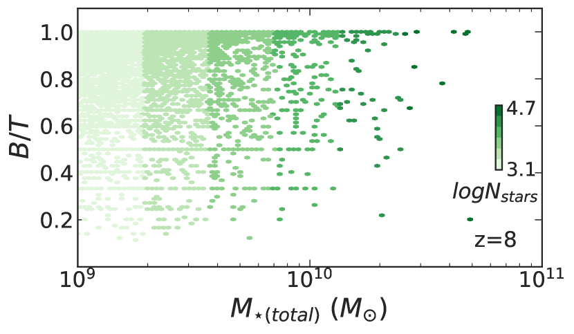
Figure 1: The relation between $B/T$ total stellar mass ($M_{\star}$) color coded according to number of star particles for each galaxy at $z=8$ in BlueTides.

2.3 Kinematic decomposition

As $\sigma$ or $M_{\star}$ in observational studies of $M_{\bullet}-\sigma$ or $M_{\bullet}-M_{\star}$ relations are often measured from the bulge component of galaxies, we perform a kinematic decomposition for the stellar particles of the galaxies in BlueTides as in Feng et al. (2015). This allows us to determine which stars are on planar circular orbits and which are associated with a bulge, in each galaxy (Vogelsberger et al., 2014; Tenneti et al., 2016), providing kinematically classified disks and bulges, and a disk to total ($D/T$) ratio for our galaxies. We perform this analysis following Abadi et al. (2003): a circularity parameter is defined for every star particle as $\kappa=j_{z}/j\left(E\right)$, where $j_{z}$ is the specific angular momentum around a selected z-axis and $j\left(E\right)$ is the possible maximum specific angular momentum of the star with the specific binding energy $E$. The star particle with $\kappa>0.7$ is identified as a disk component according to Vogelsberger et al. (2014) and Tenneti et al. (2016). Thus, the $D/T$ ratio for the stellar component of each galaxy is obtained, allowing us to calculate the bulge stellar mass and the bulge velocity dispersion for our galaxies. In Figure 1, we show the relation between $B/T=1-D/T$ (bulge to total ratio) and total stellar mass ($M_{\star}$) color coded according to number of star particles for each galaxy. According to the standard assumption $D/T<0.3$ is considered a bulge dominated galaxies (Feng et al., 2015; Tenneti et al., 2016). For galaxies with $M_{\star}>10^{9}M_{\sun}$, the number of star particles is higher than $1000$. We require this minimum number of star particles to have a reliable kinematic decomposion. For this reason, for the rest of the analysis we will only consider objects with $M_{\star}>10^{9}M_{\sun}$.

3 The global property of BH mass

We begin by investigating the global properties of BH mass ($M_{\bullet}$) from $z=8$ to $z=12$ in BlueTides. We choose a BH population with $M_{\bullet}>1.5\times 10^{6}M_{\sun}$ which is roughly twice the BH seed mass ( $M_{\rm\bullet,seed}=7.2\times 10^{5}M_{\sun}$), in order to minimize any possible influence of the seeding prescription on our analysis.

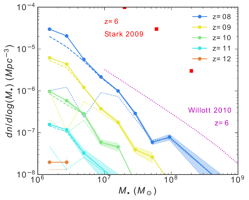
Figure 2: Left panel: the relation between BH bolometric luminosity ($L_{\rm B}$) and BH mass ($M_{\bullet}$) at $z=8$ in BlueTides color coded according to the number of galaxies. The green line shows $L_{\rm B}$ with the mean Eddington ratio of our all BH population ($L_{\rm\overline{\lambda}_{\rm Edd}=0.29}$). The brown dashed and dotted lines show the X-ray luminosity $L_{X}=10^{42.5}$ and $10^{43}erg/s$ respectively according to the bolometric correction from Marconi et al. (2004). Right panel: BH mass functions in BlueTides at $z=8\sim 12$ (the solid curves). The dashed and dotted curves show the BH mass functions with thresholds of $L_{\rm X}=10^{42.5}$ and $10^{43}erg/s$ respectively at the corresponding redshift. Also, the results at $z=6$ in Willott et al. (2010) and Volonteri & Stark (2011) are shown.

3.1 BH mass function and bolometric luminosity

We first look at the bolometric luminosity ($L_{\rm B}$) of BH population in BlueTides at $z=8$ in the left panel in Figure 2. The brown dashed and dotted lines are X-ray luminosity $L_{\rm X}=10^{42.5}$ and $10^{43}erg/s$, which are calculated by the bolometric correction in Marconi et al. (2004). These two values will be used as thresholds when studying other global properties of BH mass in this section. Statistically, there are more than $76$ and $16$ percent of our BHs with $L_{\rm X}>10^{42.5}$ and $10^{43}erg/s$ respectively. This indicates that the global quantities of BH mass is sensitive to $L_{\rm X}$ when measured from X-ray survey in observation. In addition, $L_{\rm B}$ with the mean Eddington ratio in our BH population ($\overline{\lambda}_{\rm Edd}=0.29$) is shown (the green solid line).

The right panel in Figure 2 shows BH mass functions (BHMFs) in BlueTides from $z=8$ to $z=12$ (the solid curves), as well as the ones with thresholds $L_{\rm X}>10^{42.5}$ and $10^{43}erg/s$ (the dashed and dotted curves respectively). We also show the BHMFs inferred from optical quasars at $z=6$ in Willott et al. (2010) (W10 hereafter; the purple dotted curve) and the theoretical prediction combined with observed Lyman break galaxy population (Stark et al., 2009; Volonteri & Stark, 2011) (the red squares). The slope of BHMFs in BlueTides are generally steeper than the one in W10 but similar to theoretical predictions (see Volonteri & Stark (2011) for more detail and comparison), particularly at the low mass end (which is currently unconstrained at these redshifts). In addition, the normalization of the BHMFs in BlueTides suggests that there is a larger BH population than those which have been observed from optical quasars, consistent with the claim that there is a large population of obscured accreting BHs at high-$z$.

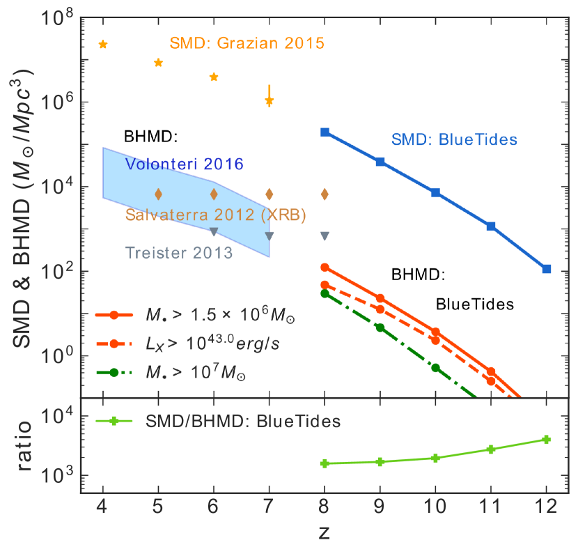
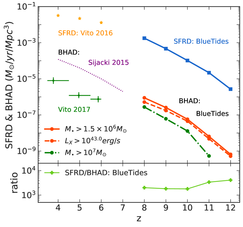
Figure 3: Left panel: the stellar mass and BH mass density (SMD and BHMD) inBlueTidesand their ratio SMD/BHMD (the green solid curve). For SMD, galaxies with $M_{\star}>10^{8}M_{\sun}$ are selected in simulation (the blue solid curve) and observation (Grazian et al. (2015); the orange stars). For BHMD, galaxies with $M_{\bullet}>1.5\times 10^{6}M_{\sun}$ (double of $M_{\rm\bullet,seed}$), with $M_{\bullet}>10^{7}M_{\sun}$, and with $L_{\rm X}>10^{43}erg/s$ are shown (the red solid, olive dash-dotted, and red dash curves respectively). The blue shaded area is the result in Volonteri & Reines (2016) and the brown diamonds and gray triangles are current upper limits from X-ray observations (Salvaterra et al., 2012; Treister et al., 2013). Right panel: the SFR and BH accretion rate density (SFRD and BHAD) in BlueTides and their ratio SFRD/BHAD (the green curve). The same thresholds are used as the left panel. Observational results in Vito et al. (2016) and Vito et al. (2018) for SFRD and BHAD are shown (the orange stars and green dots respectively), as well as the simulation prediction from Sijacki et al. (2015) (purple dotted curve; thresholds: $M_{\rm\bullet,seed}>10^{5}h^{-1}M_{\sun}$).

3.2 BH mass density and stellar mass density

The left panel in Figure 3 shows BH and galaxy stellar mass density in BlueTides from $z=8$ to $z=12$ with observations from $z=4$ to $z=7$. For stellar mass density (SMD), BlueTides (the solid blue curve) agrees with the trend from Grazian et al. (2015) (the orange stars). Galaxies with $M_{\star}>10^{8}M_{\sun}$ are selected for both cases. For BH mass density (BHMD), we report the results with two different $M_{\bullet}$ thresholds: $M_{\bullet}>1.5\times 10^{6}M_{\sun}$ ( double of $M_{\rm\bullet,seed}$ in BlueTides) and $M_{\bullet}>10^{7}M_{\sun}$ ) and with $L_{\rm X}>10^{43erg/s}$ (the red solid, olive dash-dotted, and red dash curves respectively) to show the influence from $M_{\bullet}$ and $L_{\rm X}$ thresholds. Current upper limits from X-ray observation are also presented: Salvaterra et al. (2012) (cosmic X-ray background (XRB) ) and Treister et al. (2013) (the brown diamonds and gray triangles respectively). BHMD in BlueTides complies with those upper limits (at least at $z=8$), pointing that our BH mass function is just steeper than the one in W10 but still within the upper limits from X-ray observation. In addition, results in Volonteri & Reines (2016) (the blue shade) are also included to support our BHMF, arguing that the integrated BH density depends on the $M_{\bullet}-M_{\star}$ relation.

It has been discussed that the stellar mass density exceeds the BH mass density roughly by a factor of $10^{3}$ for low-$z$. To understand the ratio of these two quantities at higher redshifts, we show the ratio by normalizing SMD to BHMD in the left panel in Figure 3 (the green solid curve). Overall, SMD grows more rapidly than the BHMD at early times. Parameterizing the ratio by an evolutionary factor $(1+z)^{\alpha}$, we find that $SMD/BHMD=1.3(1+z)^{3.1}$.

3.3 BH accretion rate density and SFR density

After BHMD and SMD, we investigate their assembly rate: the BH accretion rate density and the SFR density. The right panel in Figure 3 shows the BH accretion rate density (BHAD) again with $M_{\bullet}$ and $L_{\rm X}$ thresholds $M_{\bullet}>1.5\times 10^{6}M_{\sun}$, $M_{\bullet}>10^{7}M_{\sun}$, and $L_{\rm X}>10^{43}erg/s$ (the red solid, olive dash-dotted, and red dash curves respectively) and the SFR density (SFRD; the blue solid curve) in BlueTides from $z=8$ to $z=12$. For SFRD, we show observational result in Vito et al. (2016) (the orange stars), and on the other hand for BHAD, we not only show results from observation (Vito et al. (2018); the green dots) but also from simulation (Sijacki et al. (2015); the dotted purple curve) because it has been noticed that the prediction from simulation tends to be higher than current observation by more than an order of magnitude. It is possibly due to the difficulty of observing AGNs from deep X-ray surveys.

Similar to Section 3.2, we compare these two quantities by their ratio via normalizing SFRD to BHAD (the green curve). The ratio of the SFRD and the BHAD increases as $z$ increases and the order of which (ranging from $10^{3}$ to $10^{4}$) is close to the order of the ratio of the BHMD and the SMD in our simulation. Again, we fit the ratio as a function of $(1+z)^{\alpha}$: $SFRD/BHARD=3.4(1+z)^{2.7}$.

4 The Scaling Relations

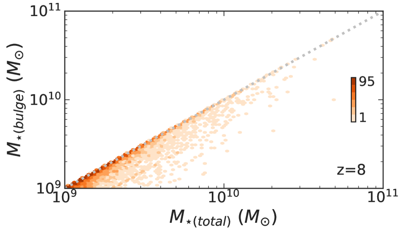
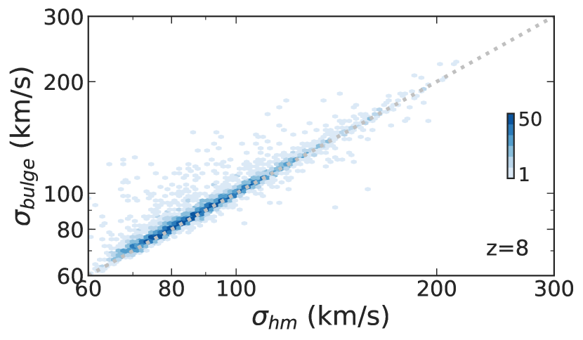
Figure 4: The top and bottom panels show $M_{\star{\rm,bulge}}$ versus $M_{\star{\rm,total}}$ and $\sigma_{\rm bulge}$ versus $\sigma_{\rm hm}$ respectively, color coded by the number of galaxies at $z=8$ in BlueTides.

4.1 Measuring $M_{\star}$ and $\sigma$

The scaling relations between BH mass and their host galaxy properties have been measured by total stellar mass ($M_{\star{\rm,total}}$) or bulge stellar mass ($M_{\star{\rm,bulge}}$) for $M_{\bullet}-M_{\star}$ relation, and by velocity dispersion of bulge stars for $M_{\bullet}-\sigma$ relation. In simulations, total or half stellar mass is available as a proxy for $M_{\star{\rm,bulge}}$. A proxy for $\sigma$ often used is the velocity dispersion within half-light (or mass) radius (as for example in Sijacki et al. (2015) and DeGraf et al. (2015)). With the dynamical disk-bulge decomposition (see Section 2.3) for the stellar components of galaxies in BlueTides, we directly have $M_{\star{\rm,bulge}}$ and $\sigma_{\rm bulge}$ in our galaxies.

The top panel in Figure 4 shows the comparison between the $M_{\star{\rm,bulge}}$ and $M_{\star{\rm,total}}$ color coded according to the number of galaxies. We find that about $82\%$ of objects are bulge-dominated with $D/T<0.3$. The bottom panel in Figure 4 shows the comparison between $\sigma_{\rm bulge}$ and $\sigma_{\rm hm}$ color coded according to the number of galaxies. Again, there is certainly a strong correlation between the two but an increased scatter above the one-to-one relation for a small number of objects, for which we have larger values of $\sigma_{\rm bulge}$ for a given $\sigma_{\rm hm}$. In particular, we find that over $94\%$ and $97\%$ of our galaxies have the difference between $\sigma_{\rm bulge}$ and $\sigma_{\rm hm}$ less than $10\%$ and $20\%$ respectively. We shall see in the next section how the detailed dynamical decomposition and the resulting $\sigma_{\rm bulge}$ and $M_{\star{\rm,bulge}}$ impact the scaling relations.

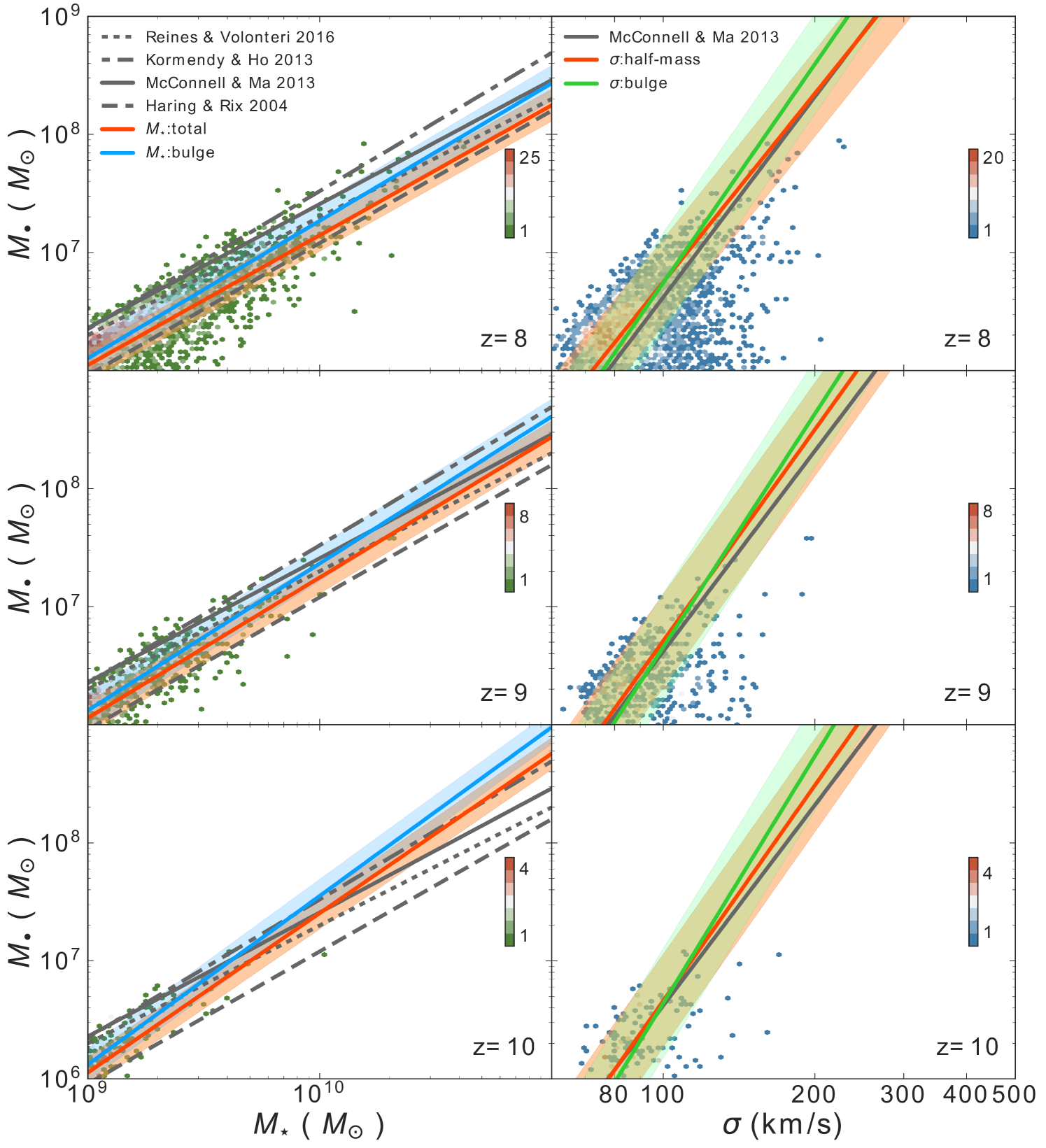
Figure 5: The scaling relations at $z=8$, $9$, and $10$ in BlueTides color coded according to the number of galaxies. Left panels: the $M_{\bullet}-M_{\star}$ relations with $M_{\star{\rm,bulge}}$ for the data points. The red and blue lines show the best-fitting relation using $M_{\star{\rm,total}}$ and $M_{\star{\rm,bulge}}$ respectively while the gray lines show the observations (Häring & Rix, 2004; McConnell & Ma, 2013; Kormendy & Ho, 2013; Volonteri & Reines, 2016). Right panels: the $M_{\bullet}-\sigma$ relations with $\sigma_{\rm bulge}$ for the data points. The red and green lines show the best-fitting relation with $\sigma_{\rm hm}$ and $\sigma_{\rm bulge}$ respectively while the gray lines show the observations in McConnell & Ma (2013). The shaded area shows the standard deviation of residuals.

Table 2: The fitting coefficients $\alpha$ and $\beta$ (normalization and slope) of equation (1), the total number of data points $N$, and the standard deviation of residuals $\epsilon$ of the scaling relations at each redshift.

		$M_{\bullet}-M_{\star{\rm,total}}$			$M_{\bullet}-\sigma_{\rm hm}$				$M_{\bullet}-M_{\star{\rm,bulge}}$			$M_{\bullet}-\sigma_{\rm bulge}$
$z$	$N$	$\alpha$	$\beta$	$\epsilon$	$\alpha$	$\beta$	$\epsilon$		$\alpha$	$\beta$	$\epsilon$	$\alpha$	$\beta$	$\epsilon$
8	8131	$8.25_{\pm 0.03}$	$1.10_{\pm 0.01}$	0.14	$8.35_{\pm 0.08}$	$5.31_{\pm 0.04}$	0.36		$8.43_{\pm 0.06}$	$1.16_{\pm 0.01}$	0.15	$8.60_{\pm 0.17}$	$6.15_{\pm 0.09}$	0.42
9	1567	$8.44_{\pm 0.08}$	$1.19_{\pm 0.01}$	0.14	$8.50_{\pm 0.23}$	$5.95_{\pm 0.12}$	0.40		$8.61_{\pm 0.14}$	$1.24_{\pm 0.02}$	0.15	$8.63_{\pm 0.47}$	$6.56_{\pm 0.24}$	0.46
10	269	$8.76_{\pm 0.20}$	$1.35_{\pm 0.02}$	0.13	$8.49_{\pm 0.54}$	$6.06_{\pm 0.28}$	0.40		$8.98_{\pm 0.37}$	$1.43_{\pm 0.04}$	0.14	$8.73_{\pm 1.24}$	$6.95_{\pm 0.63}$	0.46

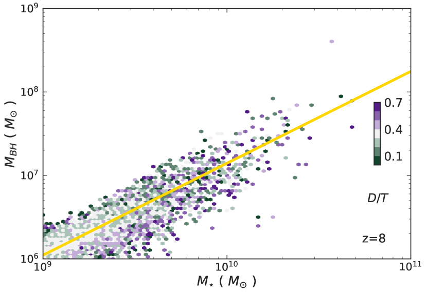
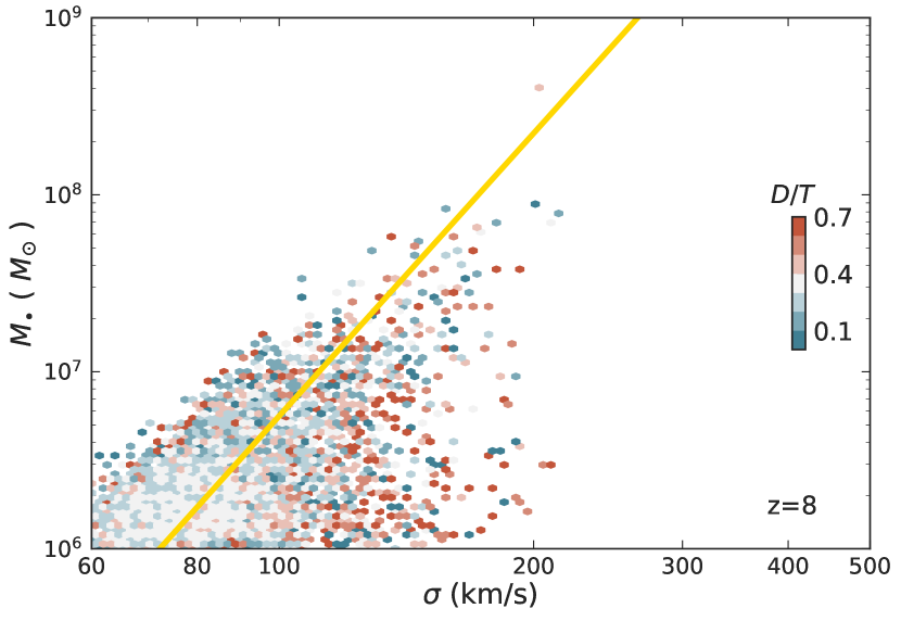
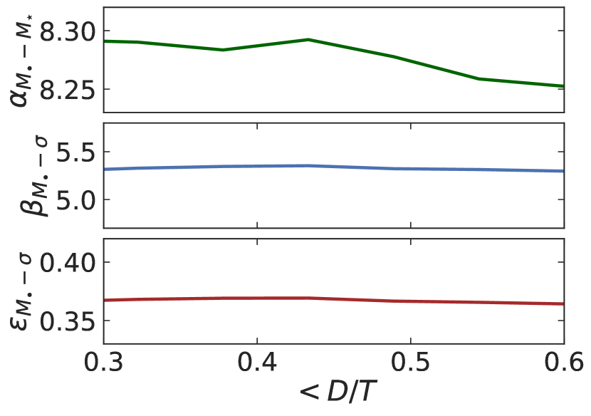
Figure 6: Top and middle panels: the $M_{\bullet}-M_{\star}$ and $M_{\bullet}-\sigma$ relations color coded according to $D/T$ at $z=8$ in BlueTides. The yellow lines show the overall fits as the ones in Figure 5. Bottom panel: $\alpha$ of $M_{\bullet}-M_{\star}$ relation and $\beta$ and $\epsilon$ of $M_{\bullet}-\sigma$ relation as functions of different limiting $D/T$.

4.2 $M_{\bullet}-M_{\star}$ and $M_{\bullet}-\sigma$ relation

Figure 5 shows the $M_{\bullet}-M_{\star}$ relation and the $M_{\bullet}-\sigma$ relation at $z=8$, $9$, and $10$ in BlueTides, color coded according to the number of galaxies. Note that the data points are shown with $M_{\star{\rm,bulge}}$ and $\sigma_{\rm bulge}$. We plot and fit only galaxies with $M_{\star}>10^{9}M_{\sun}$ where a sufficient number of star particles are available to carry out the dynamical decomposition reliably. Both scaling relations in BlueTides are best-fitted by power laws as

$$\log_{10}\left(M_{\bullet}\right)=\alpha+\beta\ \log_{10}\left(X\right),$$ (1)

where $M_{\bullet}$ is in units of $M_{\sun}$, and $X$ is $M_{\star}/10^{11}M_{\sun}$ or $\sigma/200kms^{-1}$. The fitting coefficients (normalization $\alpha$ and slope $\beta$) are summarized in Table 2, including the total number of data points $N$ and the standard deviation of the residuals $\epsilon$.

The left panels in Figure 5 show the $M_{\bullet}-M_{\star}$ relations. The red and blue lines show the best-fitting relation with $M_{\star{\rm,total}}$ and $M_{\star{\rm,bulge}}$ respectively while the gray lines show the observations: Häring & Rix (2004), McConnell & Ma (2013) and Kormendy & Ho (2013) with bulge stellar mass and elliptical samples while Volonteri & Reines (2016) with total stellar mass. Our simulation provides the $M_{\bullet}-M_{\star}$ relation in the form of $\log_{10}(M_{\bullet})=8.25+1.10\ \log_{10}(M_{\star}/10^{11}M_{\sun})$ with $M_{\star{\rm,total}}$ at $z=8$, suggesting that the slopes are consistent with the observations but the normalizations are lower than most observations except for the one in Häring & Rix (2004). Both $\alpha$ and $\beta$ with $M_{\star{\rm,total}}$ (the red lines) are lower than the ones with $M_{\star{\rm,bulge}}$ (the blue lines) across all three redshifts, and both get steeper as $z$ is higher. The standard deviation of the residuals ($\epsilon$) is shown as the shaded area.

The right three panels in Figure 5 show the $M_{\bullet}-\sigma$ relations. The red and green lines show the best-fitting relation with $\sigma_{\rm hm}$ and $\sigma_{\rm bulge}$ respectively while the gray lines show the observations in McConnell & Ma (2013). Our simulation provides the $M_{\bullet}-\sigma$ relation with $\sigma_{\rm hm}$ as $\log_{10}(M_{\bullet})=8.35+5.31\ \log_{10}(\sigma/200kms^{-1})$ at $z=8$, which is consistent with the results of McConnell & Ma (2013). We note that both $\alpha$ and $\beta$ using $\sigma_{\rm hm}$ (the red lines) are lower by $\sim 3\%$ and $\sim 10\%$, respectively than the ones with $\sigma_{\rm bulge}$ (the blue lines) across all three redshifts, and both get steeper with increasing $z$ . Moreover, $M_{\bullet}-\sigma$ relations with $\sigma_{\rm bulge}$ are higher than local measurements. $\epsilon$ is shown as the shaded area and, more importantly, $M_{\bullet}-\sigma$ relation shows a larger scatter than the $M_{\bullet}-M_{\star}$ relation ($\epsilon\sim 0.4$ and $\epsilon\sim 0.1$ respectively) in our simulations. We will examine this in Section 5.

For most observational results, the scaling relations are established with bulge-dominated galaxies. Here, we report how the relations change in our simulation with bulge-dominated galaxies ($D/T<0.3$). In the top two panels in Figure 6, we show both relations color coded according to the $D/T$ ratio. In the bottom panels, we show $\alpha$ of $M_{\bullet}-M_{\star}$ relations and $\beta$ and $\epsilon$ of $M_{\bullet}-\sigma$ relations as functions of limiting $D/T$. We find that the relations hardly change even with different $D/T$, even for the bulge-dominated regime $D/T<0.3$.

5 The slope and scatter in the scaling relations

We have shown that the high-z relation is consistent with the locally measured ones (both in slope and normalization). However here we wish to investigate possible selection effects and/or physical parameters that may affect the slope and scatter in the scaling relations (Figure 5 and Table 2). In particular, we have found that there is a more significant scatter in the $M_{\bullet}-\sigma$ relation (larger than in local measurements) than the $M_{\bullet}-M_{\star}$ relation. The relatively large scatter in the $M_{\bullet}-\sigma$ relation appears to be due to a significant amount of objects that lie below the main relation: galaxies with relative high $\sigma$ compared to their relative low $M_{\bullet}$. Note that $M_{\star}$ denotes $M_{\star{\rm,total}}$ and $\sigma$ denotes $\sigma_{\rm hm}$ hereafter unless stated otherwise.

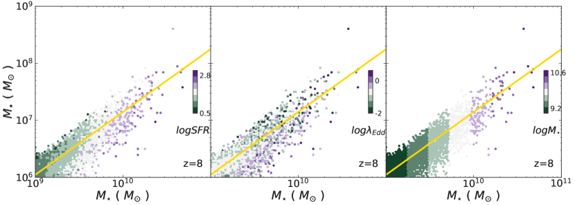
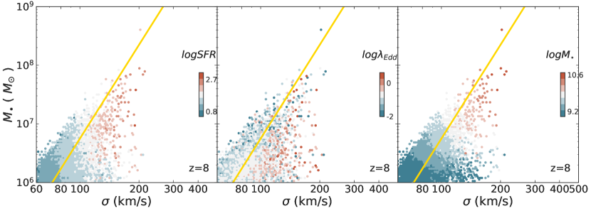
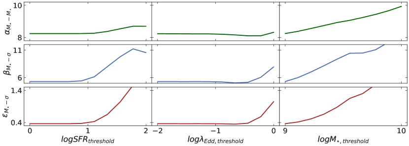
Figure 7: Top and middle panels: the $M_{\bullet}-M_{\star}$ and $M_{\bullet}-\sigma$ relations color coded according to $SFR$, $\lambda_{\rm Edd}$, and $M_{\star}$ (from left to right respectively) at $z=8$ in BlueTides. The yellow lines show the overall fits as the ones in Figure 5. Bottom panel: $\alpha$ of $M_{\bullet}-M_{\star}$ relation and $\beta$ and $\epsilon$ of $M_{\bullet}-\sigma$ relation as functions of different thresholds of $SFR$, $\lambda_{\rm Edd}$, and $M_{\star}$ from left to right respectively.

5.1 $SFR$, $\lambda_{\rm Edd}$, and $M_{\star}$ dependence

Here, we examine the dependency of the scaling relations at $z=8$ on galaxy properties. The top and middle panels in Figure 7 show the $M_{\bullet}-M_{\star}$ and $M_{\bullet}-\sigma$ relations for threshold samples selected for (from the left to right) $SFR$ (a proxy for the galaxy luminosity), stellar mass ($M_{\star}$), and BH accretion rate, in units of Eddington (Eddington ratio $\lambda_{\rm Edd}$; a proxy for the AGN luminosity), while the yellow line is the best fit from all galaxies. We wish to examine if the above selection thresholds may have an influence on the slopes, normalization and scatter in the relations.

The bottom panels of Figure 7 show the variation in normalization $\alpha$ of the $M_{\bullet}-M_{\star}$ relation and in the slope $\beta$ and scatter $\epsilon$ of the $M_{\bullet}-\sigma$ relation as functions of thresholds of $SFR$, $\lambda_{\rm Edd}$, and $M_{\star}$. We find that the normalization ($\alpha$) of $M_{\bullet}-M_{\star}$ relation increases slightly for higher thresholds of $SFR$ and $M_{\star}$ (while it is not sensitive to the Eddington rate/AGN luminosity). The slope ($\beta$) of $M_{\bullet}-\sigma$ increases for higher thresholds of $SFR$ and $M_{\star}$, indicating that selection effects at these high redshifts (which typically bias samples toward high $SFR$ and $M_{\star}$ objects) are likely to play an important role and lead to biased interpretations of evolutionary effects in these relations when compared to those seen at low-$z$. The scatter also tends to increase particularly when high $SFR$ or high $M_{\star}$ samples are selected (which populate the $\sigma\geq 200$ km/s range).

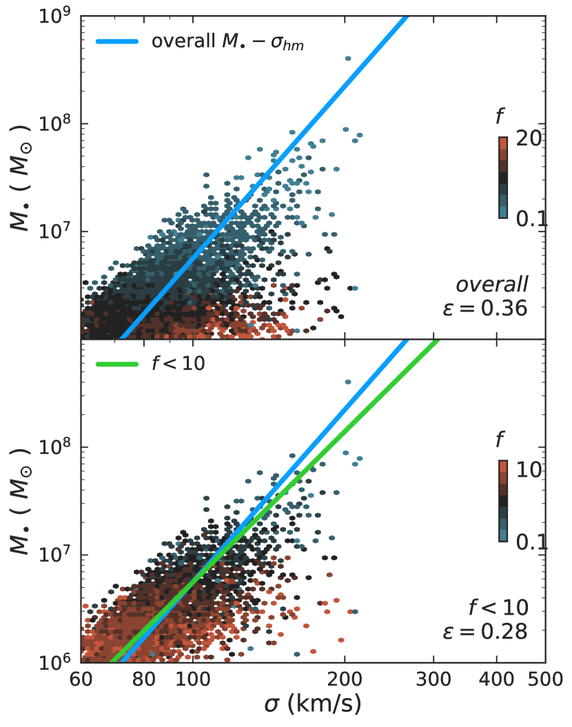
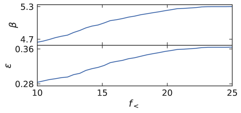
Figure 8: Top and middle panels: the $M_{\bullet}-\sigma$ relation at $z=8$ color coded according to the gas-to-stellar ratio ($f$). The blue and green lines are the best fits with overall galaxies and galaxies with $f<10$ respectively. Bottom panel: $\beta$ and $\epsilon$ of $M_{\bullet}-\sigma$ relation at $z=8$ as functions of limiting $f$.

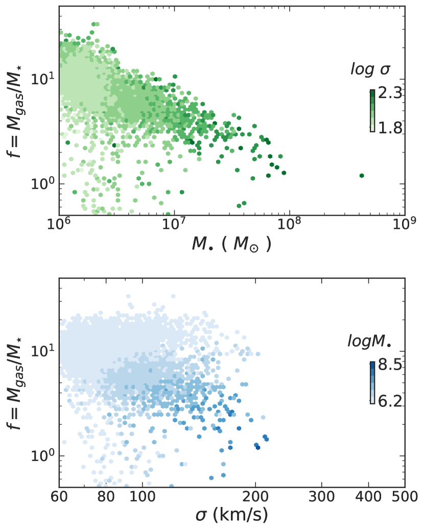
Figure 9: The relations between $f=M_{\rm gas}/M_{\star}$, $M_{\bullet}$, and $\sigma$ color coded according to $\sigma$ and $M_{\bullet}$ (top and bottom respectively).

5.2 The gas fraction: $f=M_{gas}/M_{\star}$

In Section 5.1, we have examined the dependence of the scaling relation on the various galaxy or AGN parameters; none of them helps to explain the relatively large intrinsic scatter in the $M_{\bullet}-\sigma$ relation. Here, we test for the effects due to the large range and high value of gas fraction in the high-$z$ galaxies and how that may affect the $M_{\bullet}-\sigma$ relation.

We use the gas-to-stellar ratio ($f$) to measure the gas fraction in our galaxies in BlueTides. Figure 8 shows the $M_{\bullet}-\sigma$ relation at $z=8$ color coded according to $f$. We find that the gas fraction in galaxies $f$ has a significant impact on the scatter of the $M_{\bullet}-\sigma$ relation. In particular, the scatter is significantly reduced for galaxies with a smaller value of $f$. We find that $\epsilon$ decreases significantly from $0.36$ (all galaxies) to $0.28$ (with $f<10$) while the slope of the relation ($\beta$) decreases from $5.31$ (all galaxies) to $4.64$ (with $f<10$). We further illustrate this trend of decreasing of $\epsilon$ and $\beta$ with different limiting $f$, in the bottom panel in Figure 8. Lower gas fractions are indeed more representative of local galaxies, which have been used to measure the $M_{\bullet}-\sigma$.

The decrease of both $\epsilon$ and $\beta$ with the lower limiting $f$ implies that objects with higher $\sigma$ but lower $M_{\bullet}$ are those that have higher $f$. To look into the relations between $f$, $M_{\bullet}$, and $\sigma$, we show Figure 9, color coded according to $\sigma$ and $M_{\bullet}$ respectively. The top panel indicates a trend between a decreasing $f$ at increasing $M_{\bullet}$. Gas fractions of galaxies decrease as BH masses are high/reach the relation, indicating that BH growth is quenched/self-regulated due to AGN feedback. The galaxies with higher $\sigma$ but lower $M_{\bullet}$ are indeed those that have larger $f$ (the light blue area in the bottom panel), which results in that the $M_{\bullet}-\sigma$ relation is more scattered if there is no limiting $f$ applied. These are relatively sizeable galaxies where significant BH growth is still occurring (see also Figure 10 and objects are still moving toward the relation (feedback has not yet saturated the BH growth). Such an actively growing BH population is indeed rare among the sample of quiescent local BHs.

6 The assembly history

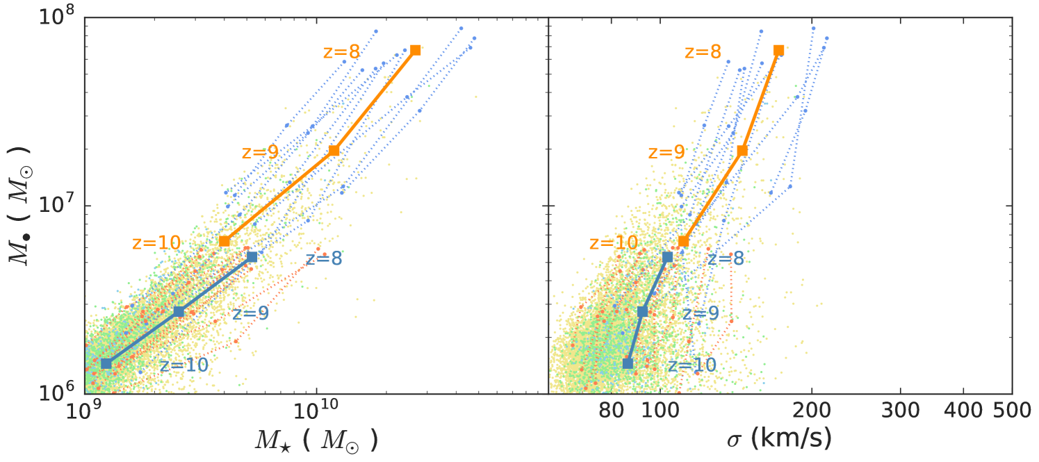
Figure 10: The left and the right panels show the growth history on $M_{\bullet}-M_{\star}$ and $M_{\bullet}-\sigma$ planes of our galaxies from $z=8$ to $z=10$ respectively. The blue and orange dashed curves show the evolution of $\sim 10$ galaxies with $M_{\bullet}>5\times 10^{7}M_{\sun}$ and another $\sim 10$ galaxies with $M_{\bullet}\sim 5\times 10^{6}M_{\sun}$. The blue and orange thick curves demonstrate the average growth history for either groups.

To further investigate how the $M_{\bullet}-M_{\star}$ and $M_{\bullet}-\sigma$ relations are established we trace the evolution of $\sim 200$ black holes (from $z\sim 10$ to $z\sim 8$) and their hosts. In Figure 10, we show sample tracks on the $M_{\bullet}-M_{\star}$ and $M_{\bullet}-\sigma$ plane from $z=10$ to $z=8$. The solid lines shown in orange and blue show the average track in the evolution for higher mass (with $M_{\bullet}\gtrsim 5\times 10^{7}M_{\sun}$) and lower mass (with $M_{\bullet}\lesssim 5\times 10^{6}M_{\sun}$) respectively. The tracks in the $M_{\bullet}-\sigma$ plane suggest a slightly steeper growth in the low mass galaxies compared to the high mass galaxies. This likely indicates a fast growth of the black hole mass at approximately fixed values of $\sigma$ up to the point where the galaxies reach the average relation.

To characterize the overall evolution in these planes, we parameterize the growth of $M_{\bullet}$, $M_{\star}$, and $\sigma$ as

$$M_{\bullet}\left(z\right)\propto\left(1+z\right)^{\gamma_{\bullet}}$$

$$M_{\star}\left(z\right)\propto\left(1+z\right)^{\gamma_{\star}}$$ (2)

$$\sigma\left(z\right)\propto\left(1+z\right)^{\gamma_{\sigma}}.$$

where the exponents are $\gamma_{\bullet}=-9.1\pm 1.0$, $\gamma_{\star}=-8.1\pm 2.2$, and $\gamma_{\sigma}=-1.6\pm 0.8$, (the error bars are standard deviation errors). Note that $\gamma_{\bullet}/\gamma_{\star}\sim 1.1$ and $\gamma_{\bullet}/\gamma_{\sigma}\sim 5.7$, which is consistent with the slope of the scaling relation shown in Table 2 (if we use Eqs. (6) and eliminate $(1+z)$, then $\gamma_{\bullet}/\gamma_{\star}\sim\beta_{\rm M_{\bullet}-M_{\star}}$ and $\gamma_{\bullet}/\gamma_{\sigma}\sim\beta_{\rm M_{\bullet}-\sigma}$). This suggests that, on average, the redshift evolution of these black holes traces the overall scaling relation (at a given redshift), with commensurate growth in black hole mass and stellar mass.

We now take a step further and look into two distinct mass regimes of the above sample of 200 BHs: 1) A low mass range of BHs with $M_{\bullet}<5\times 10^{6}M_{\sun}$, and 2) A high mass range of BHs with $M_{\bullet}>1\times 10^{7}M_{\sun}$. We note that, as discussed in the previous section, the lower mass subsample has more scatter in the $M-\sigma$ relation (see Section 4). We find that $\gamma_{\bullet}=-5.7\pm 3.5$, $\gamma_{\sigma}=-0.72\pm 0.49$ and $\gamma_{\bullet}=-10\pm 2.6$, $\gamma_{\sigma}=-1.8\pm 0.5$ for low mass and high mass subsamples respectively; therefore, the higher mass BHs have steeper increase in both $M_{\bullet}$ and $\sigma$, as is clearly illustrated in Figure 10. Interestingly, we also find $\gamma_{\bullet}/\gamma_{\sigma}\sim 7.9$, which is higher than the slope of the overall fit of the $M-\sigma$ relation in Section 4, suggesting that indeed these lower mass BHs tend to grow their black holes faster than their velocity dispersion and saturate their growth as they move closer to the mean relation. This behavior can then potentially lead to a decrease in the scatter in the relation at the low redshifts, where most black holes and galaxies have low gas fractions and have quenched their growth and star formation (particularly in the bulge dominated samples where the relations are typically measured). For the high mass sample, $\gamma_{\bullet}/\gamma_{\sigma}\sim 5.55$ which is consistent with the slope of the overall fit of the $M-\sigma$ relation, so that high mass objects continue to move along the relation.

7 Conclusions

We investigate the global properties of supermassive black holes at high redshifts ($z\sim 8$, $9$, $10$), which include scaling relations w.r.t properties of their host galaxies ($\sigma$, $M_{\star}$) and their redshift evolution using the BlueTides simulation. The bolometric luminosity of BHs span more than two orders of magnitude around a mean of $0.3$ of the Eddington luminosity. The BH mass functions in our simulation tend to have steeper slopes compared to the one inferred at $z=6$ measured from optical quasars. While this may be due to obscuration, we find that it is consistent with the large range of luminosities spanned and the flux cuts implied by observations. We have also shown that the BH mass density and BH accretion rate are broadly consistent with current observational constraints at the highest redshifts ($z\sim 7$).

The scaling relations, $M_{\bullet}-M_{\star}$, $M_{\bullet}-\sigma$ predicted by BlueTides reveal that correlations between the growth of black holes and their host galaxies persist at high-$z$ ($z=8$ to $z=10$), with the slopes and normalizations consistent with published relations at low-$z$. For the scatter, we find that the $M_{\bullet}-\sigma$ relation has a significantly higher scatter compared to current measurements as well as the $M_{\bullet}-M_{\star}$ relation. We further show that this large scatter can be primarily attributed to the gas-to-stellar ratio ($f=M_{\rm gas}/M_{\star}$), wherein we observe a significant decrease in the scatter ($\epsilon=0.36$ to $\epsilon=0.28$) upon exclusion of galaxies with $f=M_{\rm gas}/M_{\star}>10$. Such high gas fraction systems have the largest star formation rates and black hole accretion rates indicating that these fast-growing systems have not yet converged to the relation.

We also find that the assembly history of the evolution of BHs on $M_{\bullet}-M_{\star}$ and $M_{\bullet}-\sigma$ planes is, on an average, consistent with the corresponding scaling relations; in other words, the average trajectory of the evolution of BHs traces the mean scaling relations well.

References

- Abadi et al. (2003) Abadi M. G., Navarro J. F., Steinmetz M., Eke V. R., 2003, ApJ, 591, 499
- Bañados et al. (2017) Bañados E., et al., 2017, preprint, (arXiv:1712.01860)
- Battaglia et al. (2013) Battaglia N., Trac H., Cen R., Loeb A., 2013, ApJ, 776, 81
- Bennert et al. (2010) Bennert V. N., Treu T., Woo J.-H., Malkan M. A., Le Bris A., Auger M. W., Gallagher S., Blandford R. D., 2010, ApJ, 708, 1507
- Bhowmick et al. (2017) Bhowmick A. K., Di Matteo T., Feng Y., Lanusse F., 2017, preprint, (arXiv:1707.02312)
- Bondi (1952) Bondi H., 1952, MNRAS, 112, 195
- Bondi & Hoyle (1944) Bondi H., Hoyle F., 1944, MNRAS, 104, 273
- Bower et al. (2006) Bower R. G., Benson A. J., Malbon R., Helly J. C., Frenk C. S., Baugh C. M., Cole S., Lacey C. G., 2006, MNRAS, 370, 645
- Buchner et al. (2015) Buchner J., et al., 2015, ApJ, 802, 89
- Ciotti et al. (2009) Ciotti L., Ostriker J. P., Proga D., 2009, ApJ, 699, 89
- Croton et al. (2006) Croton D. J., et al., 2006, MNRAS, 367, 864
- DeGraf et al. (2015) DeGraf C., Di Matteo T., Treu T., Feng Y., Woo J.-H., Park D., 2015, MNRAS, 454, 913
- Di Matteo et al. (2005) Di Matteo T., Springel V., Hernquist L., 2005, Nature, 433, 604
- Di Matteo et al. (2008) Di Matteo T., Colberg J., Springel V., Hernquist L., Sijacki D., 2008, ApJ, 676, 33
- Di Matteo et al. (2017) Di Matteo T., Croft R. A. C., Feng Y., Waters D., Wilkins S., 2017, MNRAS, 467, 4243
- Fan et al. (2006) Fan X., et al., 2006, AJ, 132, 117
- Fanidakis et al. (2011) Fanidakis N., Baugh C. M., Benson A. J., Bower R. G., Cole S., Done C., Frenk C. S., 2011, MNRAS, 410, 53
- Faucher-Giguère et al. (2009) Faucher-Giguère C.-A., Lidz A., Zaldarriaga M., Hernquist L., 2009, ApJ, 703, 1416
- Feng et al. (2015) Feng Y., Di Matteo T., Croft R., Tenneti A., Bird S., Battaglia N., Wilkins S., 2015, ApJ, 808, L17
- Feng et al. (2016) Feng Y., Di-Matteo T., Croft R. A., Bird S., Battaglia N., Wilkins S., 2016, MNRAS, 455, 2778
- Fiore et al. (2012) Fiore F., et al., 2012, A&A, 537, A16
- Gebhardt et al. (2000) Gebhardt K., et al., 2000, ApJ, 539, L13
- Grazian et al. (2015) Grazian A., et al., 2015, A&A, 575, A96
- Gültekin et al. (2009) Gültekin K., et al., 2009, ApJ, 698, 198
- Häring & Rix (2004) Häring N., Rix H.-W., 2004, ApJ, 604, L89
- Hinshaw et al. (2013) Hinshaw G., et al., 2013, ApJS, 208, 19
- Hirschmann et al. (2010) Hirschmann M., Khochfar S., Burkert A., Naab T., Genel S., Somerville R. S., 2010, MNRAS, 407, 1016
- Hopkins (2013) Hopkins P. F., 2013, MNRAS, 428, 2840
- Hoyle & Lyttleton (1939) Hoyle F., Lyttleton R. A., 1939, Proceedings of the Cambridge Philosophical Society, 35, 405
- Jahnke & Macciò (2011) Jahnke K., Macciò A. V., 2011, ApJ, 734, 92
- Jiang et al. (2009) Jiang L., et al., 2009, AJ, 138, 305
- Katz et al. (1996) Katz N., Weinberg D. H., Hernquist L., 1996, ApJS, 105, 19
- Khandai et al. (2015) Khandai N., Di Matteo T., Croft R., Wilkins S., Feng Y., Tucker E., DeGraf C., Liu M.-S., 2015, MNRAS, 450, 1349
- King (2003) King A., 2003, ApJ, 596, L27
- Kormendy & Ho (2013) Kormendy J., Ho L. C., 2013, ARA&A, 51, 511
- Krumholz & Gnedin (2011) Krumholz M. R., Gnedin N. Y., 2011, ApJ, 729, 36
- Lauer et al. (2007) Lauer T. R., Tremaine S., Richstone D., Faber S. M., 2007, ApJ, 670, 249
- Magorrian et al. (1998) Magorrian J., et al., 1998, AJ, 115, 2285
- Marconi et al. (2004) Marconi A., Risaliti G., Gilli R., Hunt L. K., Maiolino R., Salvati M., 2004, MNRAS, 351, 169
- McConnell & Ma (2013) McConnell N. J., Ma C.-P., 2013, ApJ, 764, 184
- Merloni et al. (2010) Merloni A., et al., 2010, ApJ, 708, 137
- Merloni et al. (2014) Merloni A., et al., 2014, MNRAS, 437, 3550
- Mortlock et al. (2011) Mortlock D. J., et al., 2011, Nature, 474, 616
- Nelson et al. (2015) Nelson D., et al., 2015, Astronomy and Computing, 13, 12
- Peng (2007) Peng C. Y., 2007, ApJ, 671, 1098
- Reines & Volonteri (2015) Reines A. E., Volonteri M., 2015, ApJ, 813, 82
- Salvaterra et al. (2012) Salvaterra R., Haardt F., Volonteri M., Moretti A., 2012, A&A, 545, L6
- Schaye et al. (2015) Schaye J., et al., 2015, MNRAS, 446, 521
- Schulze & Wisotzki (2011) Schulze A., Wisotzki L., 2011, A&A, 535, A87
- Schulze & Wisotzki (2014) Schulze A., Wisotzki L., 2014, MNRAS, 438, 3422
- Shakura & Sunyaev (1973) Shakura N. I., Sunyaev R. A., 1973, A&A, 24, 337
- Sijacki et al. (2015) Sijacki D., Vogelsberger M., Genel S., Springel V., Torrey P., Snyder G. F., Nelson D., Hernquist L., 2015, MNRAS, 452, 575
- Silk & Rees (1998) Silk J., Rees M. J., 1998, A&A, 331, L1
- Springel (2005) Springel V., 2005, MNRAS, 364, 1105
- Springel & Hernquist (2003) Springel V., Hernquist L., 2003, MNRAS, 339, 289
- Stark et al. (2009) Stark D. P., Ellis R. S., Bunker A., Bundy K., Targett T., Benson A., Lacy M., 2009, ApJ, 697, 1493
- Steinborn et al. (2015) Steinborn L. K., Dolag K., Hirschmann M., Prieto M. A., Remus R.-S., 2015, MNRAS, 448, 1504
- Tenneti et al. (2016) Tenneti A., Mandelbaum R., Di Matteo T., 2016, MNRAS, 462, 2668
- Tenneti et al. (2018) Tenneti A., Di Matteo T., Croft R., Garcia T., Feng Y., 2018, MNRAS, 474, 597
- Treister et al. (2011) Treister E., Schawinski K., Volonteri M., Natarajan P., Gawiser E., 2011, Nature, 474, 356
- Treister et al. (2013) Treister E., Schawinski K., Volonteri M., Natarajan P., 2013, ApJ, 778, 130
- Tremaine et al. (2002) Tremaine S., et al., 2002, ApJ, 574, 740
- Treu et al. (2007) Treu T., Woo J.-H., Malkan M. A., Blandford R. D., 2007, ApJ, 667, 117
- Ueda et al. (2014) Ueda Y., Akiyama M., Hasinger G., Miyaji T., Watson M. G., 2014, ApJ, 786, 104
- Vito et al. (2014) Vito F., et al., 2014, MNRAS, 441, 1059
- Vito et al. (2016) Vito F., et al., 2016, MNRAS, 463, 348
- Vito et al. (2018) Vito F., et al., 2018, MNRAS, 473, 2378
- Vogelsberger et al. (2013) Vogelsberger M., Genel S., Sijacki D., Torrey P., Springel V., Hernquist L., 2013, MNRAS, 436, 3031
- Vogelsberger et al. (2014) Vogelsberger M., et al., 2014, MNRAS, 444, 1518
- Volonteri & Reines (2016) Volonteri M., Reines A. E., 2016, ApJ, 820, L6
- Volonteri & Stark (2011) Volonteri M., Stark D. P., 2011, MNRAS, 417, 2085
- Wang et al. (2010) Wang R., et al., 2010, ApJ, 714, 699
- Waters et al. (2016a) Waters D., Wilkins S. M., Di Matteo T., Feng Y., Croft R., Nagai D., 2016a, MNRAS, 461, L51
- Waters et al. (2016b) Waters D., Di Matteo T., Feng Y., Wilkins S. M., Croft R. A. C., 2016b, MNRAS, 463, 3520
- Wilkins et al. (2016) Wilkins S. M., Feng Y., Di-Matteo T., Croft R., Stanway E. R., Bouwens R. J., Thomas P., 2016, MNRAS, 458, L6
- Wilkins et al. (2017) Wilkins S. M., Feng Y., Di Matteo T., Croft R., Lovell C. C., Waters D., 2017, MNRAS, 469, 2517
- Wilkins et al. (2018) Wilkins S. M., Feng Y., Di Matteo T., Croft R., Lovell C. C., Thomas P., 2018, MNRAS, 473, 5363
- Willott (2011) Willott C. J., 2011, ApJ, 742, L8
- Willott et al. (2010) Willott C. J., et al., 2010, AJ, 140, 546
- Woo et al. (2006) Woo J.-H., Treu T., Malkan M. A., Blandford R. D., 2006, ApJ, 645, 900