Initial conditions for Inflation in an FRW Universe

Abstract

We examine the class of initial conditions which give rise to inflation. Our analysis is carried out for several popular models including: Higgs inflation, Starobinsky inflation, chaotic inflation, axion monodromy inflation and non-canonical inflation. In each case we determine the set of initial conditions which give rise to sufficient inflation, with at least $60$ e-foldings. A phase-space analysis has been performed for each of these models and the effect of the initial inflationary energy scale on inflation has been studied numerically. This paper discusses two scenarios of Higgs inflation: (i) the Higgs is coupled to the scalar curvature, (ii) the Higgs Lagrangian contains a non-canonical kinetic term. In both cases we find Higgs inflation to be very robust since it can arise for a large class of initial conditions. One of the central results of our analysis is that, for plateau-like potentials associated with the Higgs and Starobinsky models, inflation can be realized even for initial scalar field values which lie close to the minimum of the potential. This dispels a misconception relating to plateau potentials prevailing in the literature. We also find that inflation in all models is more robust for larger values of the initial energy scale.

I Introduction

Since its inception in the early 1980’s, the inflationary scenario has emerged as a popular paradigm for describing the physics of the very early universe star80 ; guth81 ; linde82 ; alstein82 ; baumann07 . A major reason for the success of the inflationary scenario is that, in tandem with explaining many observational features of our universe – including its homogeneity, isotropy and spatial flatness, it can also account for the existence of galaxies, via the mechanism of tiny initial (quantum) fluctuations which are subsequently amplified through gravitational instability mukhanov81 ; hawking82 ; star82 ; guth-pi82 .

An important issue that needs to be addressed by a successful model of inflation is whether the universe can inflate starting from a sufficiently large class of initial conditions. This issue was affirmatively answered for chaotic inflation in the early papers belinsky85 ; belinsky88 . Since then the inventory of inflationary models has rapidly increased. In this paper we attempt to generalize the analysis of belinsky85 ; belinsky88 to other popular inflationary models including Higgs inflation, Starobinsky inflation etc., emphasising the distinction between power law potentials and asymptotically flat ‘plateau-like’ potentials. As we shall show, our results for asymptotically flat potentials do not provide support to the ‘$unlikeliness~{}problem$’ raised in stein13 .

Our paper is organized as follows. We introduce our method of analysis in section II. Section III discusses power law potentials and includes chaotic inflation and monodromy inflation. Section IV discusses Higgs inflation in the context of both the non-minimal as well as the non-canonical framework. Section V is devoted to Starobinsky inflation. Our results are presented in section VI.

We work in the units $c,\hbar=1$ and the reduced Planck mass is assumed to be $m_{p}=\frac{1}{\sqrt{8\pi G}}$. The metric signature is $(-,+,+,+)$. For simplicity we assume that the pre-inflationary patch which resulted in inflation was homogeneous, isotropic and spatially flat. An examination of inflation within a more general cosmological setting can be found in branden16 .

II Methodology

The action for a scalar field which couples minimally to gravity has the following general form

$$S[\phi]=\int{\rm d}^{4}x\,\sqrt{-g}\;{\cal L}(F,\phi),$$ (1)

where the Lagrangian density ${\cal L}(\phi,F)$ is a function of the field $\phi$ and the kinetic term

$$F=\frac{1}{2}\partial_{\mu}\phi\;\partial^{\mu}\phi.$$ (2)

Varying (1) with respect to $\phi$ results in the equation of motion

$$\frac{\partial{\cal L}}{\partial\phi}-\left(\frac{1}{\sqrt{-g}}\right)\partial_{\mu}\left(\sqrt{-g}\frac{\partial{\cal L}}{\partial\left(\partial_{\mu}\phi\right)}\right)=0.$$ (3)

The energy-momentum tensor associated with the scalar field is

$$T^{\mu\nu}=\left(\frac{\partial{\cal L}}{\partial F}\right)\,\left(\partial^{\mu}\phi\;\partial^{\nu}\phi\right)-g^{\mu\nu}\,{\cal L}~{}.$$ (4)

Specializing to a spatially flat FRW universe and a homogeneous scalar field, one gets

$${\rm d}s^{2}=-{\rm d}t^{2}+a^{2}(t)\;\left[{\rm d}x^{2}+{\rm d}y^{2}+{\rm d}z^{2}\right],$$ (5)

$$T^{\mu}_{\;\>\;\nu}=\mathrm{diag}\left(-\rho_{{}_{\phi}},p_{{}_{\phi}},p_{{}_{\phi}},p_{{}_{\phi}}\right),$$ (6)

where the energy density, $\rho_{{}_{\phi}}$, and pressure, $p_{{}_{\phi}}$, are given by

$$\rho_{{}_{\phi}} = \left(\frac{\partial{\cal L}}{\partial F}\right)\,(2\,F)-{\cal L},$$ (7)

$$p_{{}_{\phi}} = {\cal L},$$ (8)

and $F=-({\dot{\phi}}^{2}/2)$. The evolution of the scale factor $a(t)$ is governed by the Friedmann equations:

$$\left(\frac{\dot{a}}{a}\right)^{2} = \left(\frac{8\pi G}{3}\right)\rho_{{}_{\phi}},$$ (9)

$$\frac{\ddot{a}}{a} = -\left(\frac{4\pi G}{3}\right)\left(\rho_{{}_{\phi}}+3\,p_{{}_{\phi}}\right),$$ (10)

where $\rho_{{}_{\phi}}$ satisfies the conservation equation

$${\dot{\rho}_{{}_{\phi}}}=-3\,H\left(\rho_{{}_{\phi}}+p_{{}_{\phi}}\right),~{}~{}H\equiv\frac{\dot{a}}{a}~{}.$$ (11)

For a canonical scalar field

$${\cal L}(F,\phi)=-F-V(\phi),$$ (12)

Substituting (12) into (7) and (8), we find

$$\rho_{{}_{\phi}} = \frac{1}{2}{\dot{\phi}}^{2}+\;V(\phi),$$

$$p_{{}_{\phi}} = \frac{1}{2}{\dot{\phi}}^{2}-\;V(\phi),~{}~{}$$ (13)

consequently the two Friedmann equations (9) and (10) become

$$H^{2} = \frac{8\pi G}{3}\left[\frac{1}{2}{\dot{\phi}}^{2}+\;V(\phi)\right]~{},$$ (14)

$$\frac{\ddot{a}}{a} = -\frac{8\pi G}{3}\left[{\dot{\phi}}^{2}-\;V(\phi)\right]~{}.$$ (15)

Noting that ${\dot{H}}+H^{2}={\ddot{a}}/a$ one finds ${\dot{H}}=-4\pi G{\dot{\phi}}^{2}<0$, which informs us that the expansion rate is a monotonically decreasing function of time for canonical scalar fields which couple minimally to gravity. The scalar field equation of motion follows from (3)

$${\ddot{\phi}}+3\,H{\dot{\phi}}+V^{\prime}(\phi)=0.$$ (16)

Within the context of inflation, a scalar field rolling down its potential is usually associated with the Hubble slow roll parameters baumann07

$$\epsilon_{H}=2m_{p}^{2}\left(\frac{H^{\prime}(\phi)}{H(\phi)}\right)^{2},~{}~{}\eta_{H}=2m_{p}^{2}\frac{H^{\prime\prime}(\phi)}{H(\phi)}$$ (17)

and the potential slow-roll parameters baumann07

$$\epsilon=\frac{m_{p}^{2}}{2}\left(\frac{V^{\prime}}{V}\right)^{2},~{}~{}\eta=m_{p}^{2}\frac{V^{\prime\prime}}{V}.$$ (18)

For small values of these parameters $\epsilon_{H}\ll 1,\eta_{H}\ll 1$, one finds $\epsilon_{H}\simeq\epsilon$ and $\eta_{H}\simeq\eta-\epsilon$. The expression for $\epsilon_{H}$ in (17) can be rewritten as $\epsilon_{H}=-\frac{\dot{H}}{H^{2}}$ which implies that the universe accelerates, ${\ddot{a}}>0$, when $\epsilon_{H}<1$. For the scalar field models discussed in this paper ${\dot{H}}=-4\pi G{\dot{\phi}}^{2}$ so that $\epsilon_{H}=4\pi G{\dot{\phi}}^{2}/{H^{2}}$, which reduces to $\epsilon_{H}\simeq\frac{3}{2}{\dot{\phi}}^{2}/V$ when ${\dot{\phi}}^{2}\ll V$.

The slow-roll parameters play an important role in determining the spectral index of scalar perturbations, since, $n_{{}_{S}}-1=-6\epsilon+2\eta$. Observations indicate CMB $n_{{}_{S}}\simeq 0.97$ which suggests that $\epsilon,\eta\ll 1$ on scales associated with the present cosmological horizon. The fact that $\epsilon,\eta$ are required to be rather small might appear to imply that successful inflation can only arise under a very restricted set of initial conditions, namely those for which ${\dot{\phi}}^{2}/V(\phi)\ll 1$. This need not necessarily be the case. As originally demonstrated in the context of chaotic inflation belinsky85 ; belinsky88 , a scalar field rolling down a power law potential can arrive at the attractor trajectory $\epsilon,\eta\ll 1$ from a very wide range of initial conditions. In this paper we shall apply the methods developed in belinsky85 ; belinsky88 ; felder02 to several inflationary models with power law and plateau-like potentials in order to assess the impact of initial conditions on these models.

In addition to the field equations developed earlier, we shall find it convenient to work with the parameter

$$N_{e}=\log{\frac{a(t_{\rm end})}{a(t_{\rm initial})}}={\int_{t_{i}}^{t_{e}}Hdt}\equiv-\int^{\phi}_{\phi_{{}_{e}}}\left(\frac{H}{\dot{\phi}}\right){\rm d}\,\phi$$ (19)

which describes the number of inflationary e-foldings since the onset of inflation. For our purpose it will also be instructive to rewrite the Friedman equation (14) as

$$R^{2}=X^{2}+Y^{2}$$ (20)

where

$$R=\sqrt{6}\frac{H}{m_{p}},~{}~{}X=\hat{\phi}\frac{\sqrt{2V(\phi)}}{m_{p}^{2}},~{}~{}Y=\frac{1}{m_{p}^{2}}\frac{d\phi}{dt},$$ (21)

where $\hat{\phi}=\frac{\phi}{|\phi|}$ is the sign of $\phi$ (this definition ensures that $X$ and $\phi$ have the same sign). Clearly, holding $R$ fixed and varying $X$ and $Y$, one arrives at a set of initial conditions which satisfy the constraint equation (20) defining the boundary of a circle of radius $R$. Adequate inflation is then qualified by the range of initial values of $X$ and $Y$ for which the universe inflates by at least 60 e-foldings, i.e.  $N_{e}\geq 60$.

We commence our discussion of inflationary models by an analysis of power law potentials which are usually associated with Chaotic inflation linde83 ; belinsky88 .

III Inflation with Power-law Potentials

III.1 Chaotic Inflation

We first consider the potential linde83

$$V(\phi)=\frac{1}{2}m^{2}\phi^{2}$$ (22)

where $m\simeq 5.97\times 10^{-6}m_{p}$ is assumed, in agreement with observations of the cosmic microwave background CMB ; linde06 (see Appendix A) . The generality of this model is studied by plotting the phase-space diagram ($Y$ vs $X$) and determining the region of initial conditions which gives rise to $N_{e}\geq 60$. Equations (15), (16), (19) have been solved numerically for different initial energy scales $H_{i}$. The phase-space diagram corresponding to $H_{i}=3\times 10^{-3}m_{p}$ is shown in figure 1.

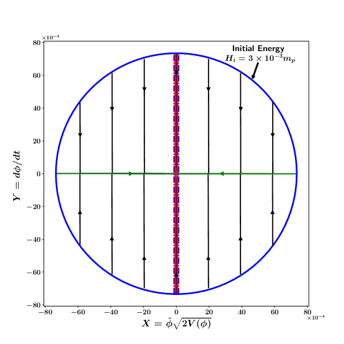
Figure 1: This figure illustrates the phase-space of chaotic inflation described by the potential (22). $Y$ ($=\dot{\phi}$) is plotted against $X$ ($=\hat{\phi}\sqrt{2V(\phi)}$) for different initial conditions all of which commence on the circumference of a circle (blue) with radius $R=\sqrt{6}H_{i}/m_{p}$ corresponding to the initial energy scale $H_{i}=3\times 10^{-3}m_{p}$. ($\hat{\phi}=\frac{\phi}{|\phi|}$ is the sign of field $\phi$.) One finds that commencing from the circle, the different inflationary trajectories rapidly converge towards one of the two inflationary separatrices (green horizontal lines). After this, the scalar field moves towards the minimum of the potential $V(\phi)$ at $X=0,Y=0$. The thin vertical central band (red) corresponds to the region in phase-space that does not lead to adequate inflation ($N_{e}<60$). This central region is shown greatly magnified in figure 2.

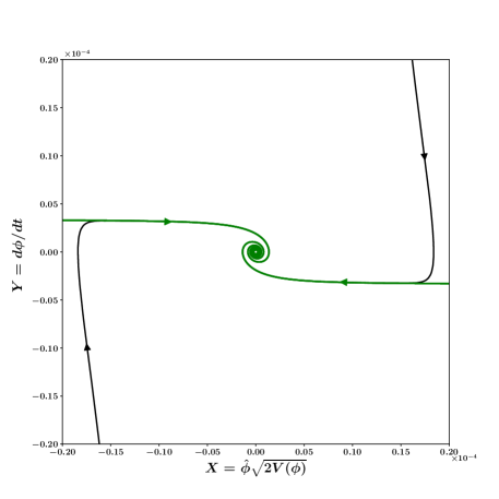
Figure 2: A zoomed-in view of the central region of figure 1. Note that $\hat{\phi}=\frac{\phi}{|\phi|}$ gives the sign of $\phi$. Inflationary trajectories (black) corresponding to different initial values of $\phi$ and $\dot{\phi}$, first converge onto the slow-roll inflationary separatrices (green horizontal lines) before winding up to spiral towards the center.

To study the effect of different energy scales on inflation, we take different values of $R$ ($\equiv\sqrt{6}H_{i}/m_{p}$) and determine the range of initial values of $\phi$ that lead to adequate inflation with $N_{e}\geq 60$. (The initial value of ${\dot{\phi}}$ is conveniently determined from the consistency relation (20).) Our results are summarized in figure 3. The solid blue lines correspond to initial values, $\phi_{i}$, which always result in adequate inflation (irrespective of the sign of ${\dot{\phi}_{i}}$). The dashed red lines corresponding to $\phi_{i}\in\big{[}-\phi_{B},-\phi_{A}\big{]}\cup\big{[}\phi_{A},\phi_{B}\big{]}$, result in adequate inflation only when ${\dot{\phi}_{i}}$ points in the direction of increasing $V(\phi)$ (represented by blue arrows). Inadequate inflation is associated with the region $\phi_{i}\in[-\phi_{A},\phi_{A}]$. If the initial scalar field value falls within this region then one does not get adequate inflation irrespective of the sign of ${\dot{\phi}_{i}}$. This region is shown in figure 3 by the solid red line. The dependence of $\phi_{A}$ and $\phi_{B}$ on the initial energy scale $H_{i}$ is given in table 1.

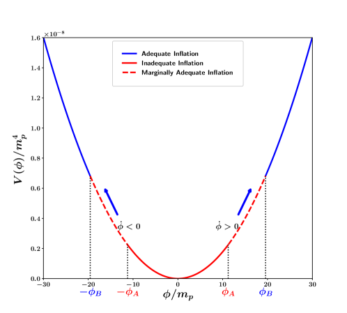
Figure 3: Initial field values, $\phi_{i}$, which lead to adequate inflation with $N_{e}\geq 60$ (blue), marginally adequate (dashed red) and inadequate (red) inflation are schematically shown for chaotic inflation (22). The blue lines represent regions of adequate inflation. Initial values of $\phi_{i}$ lying in the blue region result in adequate inflaion irrespective of the sign of $\dot{\phi}_{i}$. The red lines come in two styles: dashed/solid and correspond to the following two possibilities: (i) The solid red line represents initial values of $\phi_{i}$ for which inflation is never adequate irrespective of the direction of ${\dot{\phi}_{i}}$. (ii) In the region shown by the dashed red line one gets adequate inflation only when ${\dot{\phi}_{i}}$ is directed towards increasing values of $V(\phi)$ (shown by blue arrows). Note that only a small portion of the full potential is shown in this figure which corresponds to the initial energy scale $H_{i}=3\times 10^{-3}m_{p}$.

To determine the fraction of initial conditions that do not lead to adequate inflation (we call this ‘the degree of inadequate inflation’), we consider a uniform measure on the distribution of initial conditions for $Y_{i}(\equiv\dot{\phi}_{i})$ and $X_{i}(\equiv\hat{\phi_{i}}\sqrt{2V(\phi_{i})})$. These initial conditions are described by a circle of circumference $l=2\pi R$ with $R=\sqrt{6}H_{i}$ (in Planck units) which is illustrated in figure 4. The degree of inadequate inflation and marginally adequate inflation (corresponding respectively to $\phi_{A}$ and $\phi_{B}$ in figure 3) is $2\frac{\Delta l_{A}}{l}$ and $2\frac{\Delta l_{B}}{l}$, where $\Delta l_{A}$ and $\Delta l_{B}$ are illustrated in figure 4.

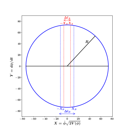
Figure 4: This figure illustrates how one can determine the degree of adequate/inadequate inflation for power law potentials characterizing chaotic inflation and monodromy inflation. The fraction of initial conditions (corresponding to $\phi_{A}$ and $\phi_{B}$ in figure 3) that leads either to inadequate inflation or marginally adequate inflation, is given by $2\frac{\Delta l_{A}}{l}$ and $2\frac{\Delta l_{B}}{l}$ respectively, where $l=2\pi R$. Adequate inflation with $N_{e}\geq 60$ is described by the fraction $1-2\frac{\Delta l_{B}}{l}$. ($\hat{\phi}=\frac{\phi}{|\phi|}$ is the sign of field $\phi$.)

The dependence of $\phi_{A}$, $\phi_{B}$ and $\frac{\Delta l_{A}}{l}$, $\frac{\Delta l_{B}}{l}$ on the commencement scale of inflation is shown in table 1. We see that the fraction of initial conditions that leads to inadequate inflation, $2\frac{\Delta l_{A}}{l}$, decreases with an increase in the initial energy scale $H_{i}$. This result is also illustrated in figures 11 and 11 where we compare chaotic inflation with monodromy inflation.

$H_{i}$ (in $m_{p}$)	$\phi_{A}$ (in $m_{p}$)	$\phi_{B}$ (in $m_{p}$)	$2\frac{\Delta l_{A}}{l}$	$2\frac{\Delta l_{B}}{l}$
$3\times 10^{-3}$	$11.22$	$19.55$	$5.80\times 10^{-3}$	$1.01\times 10^{-2}$
$3\times 10^{-2}$	$9.33$	$21.38$	$4.83\times 10^{-4}$	$1.11\times 10^{-3}$
$3\times 10^{-1}$	$7.47$	$23.27$	$3.86\times 10^{-5}$	$1.20\times 10^{-4}$

Table 1: Dependence of $\phi_{A}$, $\phi_{B}$, $\frac{\Delta l_{A}}{l}$ and $\frac{\Delta l_{B}}{l}$ on the initial energy scale $H_{i}$ for quadratic chaotic inflation; see figure 4. Here $l=2\pi R\equiv 2\pi\sqrt{6}H_{i}/m_{p}$. Note that the fraction of initial conditions which leads to inadequate inflation, $2\frac{\Delta l_{A}}{l}$, decreases as $H_{i}$ is increased. The same is true for the fraction of initial conditions giving rise to marginally adequate inflation, $2\frac{\Delta l_{B}}{l}$. The fraction of initial conditions leading to adequate inflation, with $N_{e}\geq 60$, is given by $1-2\frac{\Delta l_{B}}{l}$. Thus inflation proves to be more general for larger values of the initial energy scale $H_{i}$, since a larger initial region in phase space gives rise to adequate inflation with $N_{e}\geq 60$.

III.2 Monodromy Inflation

A straightforward extension of chaotic inflation, called Axion Monodromy, was discussed in monodromy1 ; monodromy2 in the context of String Theory and tested against the CMB in Flauger:2009ab ; CMB . The potential for monodromy inflation, which contains a monomial term along with axionic sinusoidal modulations, is given by

$$V(\phi)=V_{0}\left|\frac{\phi}{m_{p}}\right|^{p}+\Lambda^{4}\left(\cos{\frac{\phi}{f}}-1\right)$$ (23)

for $0<p\leq 1$, where $f$ is the axion decay constant while $\Lambda$ is the scale corresponding to non-perturbative effects. In this paper our focus will be on two values of $p$, namely $p=1,\frac{2}{3}$. (However our methods are very general and easily carry over to other values of $p$.)

Demanding the monotonicity of the potential (23) one gets

$$b\left|\frac{\phi}{m_{p}}\right|^{1-p}\sin{\frac{\phi}{f}}<1~{},$$ (24)

where $b=\frac{1}{p}\frac{\Lambda^{4}}{V_{0}}\frac{m_{p}}{f}$. Since $p\leq 1$ and the observable period of inflation corresponds to $\phi>m_{p}$, the monotonicity condition (24) implies $b<1$. Furthermore for $b<1$, observational constraintsFlauger:2009ab from the CMB (combined with microphysical constraints from String Theory) require $b\ll 1$ and $f\ll m_{p}$. This implies that the amplitude of modulation $\Lambda^{4}=V_{0}\frac{f}{m_{p}}bp$ is much smaller than the monomial term, i.e $\Lambda^{4}\ll V_{0}$. In other words, the sinusoidal axionic term has a negligible effect on the background dynamics so that, in an analysis of inflation, one can safely approximate the potential by its monomial term, namely

$$V(\phi)=V_{0}\left|\frac{\phi}{m_{p}}\right|^{p}~{}.$$ (25)

It is important to mention that for $p\leq 1$ the potentials (23) as well as (25) are not differentiable at the origin. This might lead to problems when $\phi$ rapidly oscillates around $\phi=0$ after the end of inflation at $\phi=\phi_{end}$. We circumvent this problem by the following useful generalization of (25)

$$V(\phi)=V_{1}\left|\frac{\phi}{\phi_{c}}\right|^{p}W(\phi)$$ (26)

where $W(\phi)=\left[1+\left(\frac{\phi_{c}}{\phi}\right)^{n}\right]^{\frac{p-2}{n}}$, $V_{1}=V_{0}\left(\phi_{c}/m_{p}\right)^{p}$ and $n>1$ is an integer (we assume $n=4$ in the ensuing analysis). In this expression the value of $\phi_{c}$ is chosen so that $V(\phi)\sim|\phi|^{p}$ for $|\phi|\gg|\phi_{c}|$ whereas $V(\phi)\sim\phi^{2}$ for $|\phi|\ll|\phi_{c}|$. It is well known that inflation ends when the slow-roll parameter $\epsilon$ in (18) grows to unity. Substituting (25) in (18) and setting $\epsilon\simeq 1$ one finds $\phi_{end}=\frac{p}{\sqrt{2}}m_{p}$ which can be used as a reference to set a value to $\phi_{c}$, namely $\phi_{c}\ll\phi_{end}$. One should note that the monomial part of the actual potentials of Axion Monodromy inflation for $p=1,~{}\frac{2}{3}$ do not have cusps at the origin. For example for $p=1$, the monomial term has the form monodromy2 $V(\phi)=V_{0}\left(\sqrt{(\phi/m_{p})^{2}+(\phi_{c}/m_{p})^{2}}-(\phi_{c}/m_{p})\right)$ which displays smooth quadratic behaviour near $\phi=0$. Likewise, for a general value of the monodromy parameter p, it is convenient to modify the potential around $\phi=0$ without changing any of the results for the background dynamics as done in mono_modify . Our introduction of a smoothing kernel $W$ in (26) follows a similar line of reasoning. It is important to emphasize that our results are quite insensitive to the values of $n$ and $\phi_{c}$ in (26) provided $\phi_{c}\ll\phi_{end}$ and $n>1$.

Next we proceed with a generality analysis for $p=1$ which will be followed by a similar analysis for $p=2/3$.

Linear Monodromy Inflation

Consider first the linear potential

$$V(\phi)=V_{0}\left|\frac{\phi}{m_{p}}\right|$$ (27)

where $V_{0}\simeq 1.97\times 10^{-10}m_{p}^{4}$ is in agreement with the CMB CMB (see Appendix A). The phase-space diagram for this potential, shown in figure 5, was obtained by solving the equations (15), (16), (19), (27) numerically, for the initial energy scale $H_{i}=3\times 10^{-3}m_{p}$.

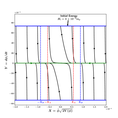
Figure 5: This figure shows a portion of the phase-space of monodromy inflation $V\propto|\phi|$. The variable $Y$ ($=\dot{\phi}$) is plotted against $X$ ($=\hat{\phi}\sqrt{2V(\phi)}$). ($\hat{\phi}=\frac{\phi}{|\phi|}$ is the sign of field $\phi$.) The initial conditions are specified on arcs which form the blue colored boundary. Note that these arcs correspond to a very small portion of the full ‘initial conditions’ circle $R$, and therefore appear to be straight lines. In this analysis we assume $R=\sqrt{6}H_{i}/m_{p}$, with $H_{i}=3\times 10^{-3}m_{p}$. We find that, commencing at the boundary, most solutions quickly converge to the two slow-roll inflationary separatrices (green horizontal lines) before travelling to the origin where $\{\dot{\phi},\phi\}=\{0,0\}$. A blow up of the central portion of this figure is shown in figure 6.

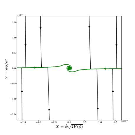
Figure 6: A zoomed-in view of the phase-space of monodromy inflation with $V\propto|\phi|$. Note that scalar field trajectories initially converge towards the slow-roll inflationary separatrices (horizontal green lines), moving from there towards $\phi=0$, where the field oscillates.

Initial values of $\phi$ that lead to adequate or inadequate inflation are schematically shown in figure 7. Inadequate inflation arises when the scalar field originates in the region $\phi_{i}\in[-\phi_{A},\phi_{A}]$, shown by solid red line. Blue lines represent initial field values $\phi_{i}\in\big{(}-\phi_{m},-\phi_{B}\big{)}\cup\big{(}\phi_{B},\phi_{m}\big{)}$, which always result in adequate inflation. Note that $\phi_{m}$ is the maximum allowed value of $\phi_{i}$ for a given initial energy scale, as determined from the consistency equations (14), (20). Initial conditions $\phi_{i}\in\big{[}-\phi_{B},-\phi_{A}\big{]}\cup\big{[}\phi_{A},\phi_{B}\big{]}$, shown by dashed red lines, lead to adequate inflation only when ${\dot{\phi}_{i}}$ points in the direction (shown by blue arrows) of increasing $V(\phi)$ . The dependence of $\phi_{A}$ and $\phi_{B}$ on the initial energy scale $H_{i}$ is shown in table 2.

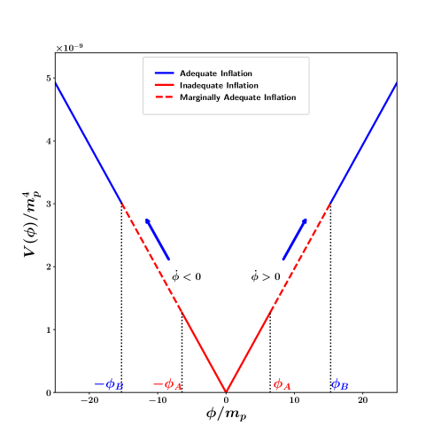
Figure 7: This figure schematically shows initial field values which result in adequate inflation with $N_{e}\geq 60$ (blue), marginally adequate (dashed red) and inadequate inflation (red) for the monodromy potential $V\propto|\phi|$. The initial energy scale is $H_{i}=3\times 10^{-3}m_{p}$. As earlier, blue lines represent regions of adequate inflation. The red lines come in two styles: dashed/solid and correspond to the two possible initial directions of ${\dot{\phi}}$. The solid red line represents initial values of $\phi$ for which inflation is never adequate irrespective of the direction of ${\dot{\phi}_{i}}$. In the region shown by the dashed line one gets adequate inflation only when ${\dot{\phi}_{i}}$ points in the direction (shown by blue arrows) of increasing $V(\phi)$. Note that only a small portion of the full potential is shown in this figure.

The values of $2\frac{\Delta l_{A}}{l}$ and $2\frac{\Delta l_{B}}{l}$ in table 2 have been determined by assuming a uniform distribution of initial values of $Y=\dot{\phi}$ and $X=\hat{\phi}\sqrt{2V(\phi)}$ on the circular boundary (20). We find that $2\frac{\Delta l_{A}}{l}$ and $2\frac{\Delta l_{B}}{l}$ decrease with an increase in $H_{i}$, as expected.

$H_{i}$ (in $m_{p}$)	$\phi_{A}$ (in $m_{p}$)	$\phi_{B}$ (in $m_{p}$)	$2\frac{\Delta l_{A}}{l}$	$2\frac{\Delta l_{B}}{l}$
$3\times 10^{-3}$	$6.45$	$15.29$	$4.37\times 10^{-3}$	$6.73\times 10^{-3}$
$3\times 10^{-2}$	$4.58$	$17.18$	$3.68\times 10^{-4}$	$7.13\times 10^{-4}$
$3\times 10^{-1}$	$2.69$	$19.06$	$2.84\times 10^{-5}$	$7.51\times 10^{-5}$

Table 2: Dependence of $\phi_{A}$, $\phi_{B}$, $\frac{\Delta l_{A}}{l}$ and $\frac{\Delta l_{B}}{l}$ on the initial energy scale $H_{i}$ for monodromy inflation $V\propto|\phi|$. Here $l=2\pi R\equiv 2\pi\sqrt{6}H_{i}/m_{p}$ and $\frac{\Delta l_{A}}{l}$, $\frac{\Delta l_{B}}{l}$ were defined in figure 4. Note that the fraction of initial conditions which leads to inadequate inflation, $2\frac{\Delta l_{A}}{l}$, decreases as $H_{i}$ is increased. The same is true for the fraction of initial conditions giving rise to marginally adequate inflation, $2\frac{\Delta l_{B}}{l}$. The fraction of initial conditions leading to adequate inflation, with $N_{e}\geq 60$, is given by $1-2\frac{\Delta l_{B}}{l}$. Thus inflation proves to be more general for larger values of the initial energy scale $H_{i}$, since a larger initial region in phase space gives rise to adequate inflation with $N_{e}\geq 60$.

Fractional Monodromy Inflation

Next we consider

$$V(\phi)=V_{0}\left|\frac{\phi}{m_{p}}\right|^{\frac{2}{3}}$$ (28)

where CMB constraints imply $V_{0}=3.34\times 10^{-10}m_{p}^{4}$ CMB (see Appendix A). The phase-space diagram for this potential, shown in figure 8, was obtained by solving the equations (15), (16), (19) numerically for the initial energy scale $H_{i}=3\times 10^{-3}m_{p}$.

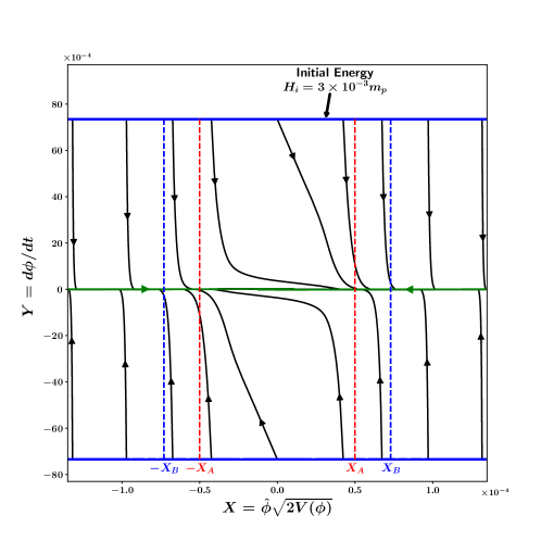
Figure 8: This figure shows a portion of the phase-space of monodromy inflation with $V\propto|\phi|^{2/3}$. The variable $Y$ ($=\dot{\phi}$) is plotted against $X$ ($=\hat{\phi}\sqrt{2V(\phi)}$). ($\hat{\phi}=\frac{\phi}{|\phi|}$ is the sign of field $\phi$.) Initial conditions are specified on arcs which form the blue colored boundary. Note that since these arcs correspond to a very small portion of the full ‘initial conditions’ circle $R$, they appear to be straight lines. As in the previous analysis for chaotic inflation we again assume $R=\sqrt{6}H_{i}/m_{p}$, with $H_{i}=3\times 10^{-3}m_{p}$. One finds that, commencing at the boundary, most solutions quickly converge to the two slow-roll inflationary separatrices (green horizontal lines) before travelling to the origin where $\{\dot{\phi},\phi\}=\{0,0\}$. A blow up of the central portion of this figure is shown in figure 9.

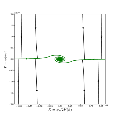
Figure 9: A zoomed-in view of the phase-space of monodromy inflation with $V\propto|\phi|^{2/3}$. One notes that the motion of the scalar field is initially towards the slow-roll inflationary separatrices (horizontal green lines) and from there towards $\phi=0$, where the field oscillates.

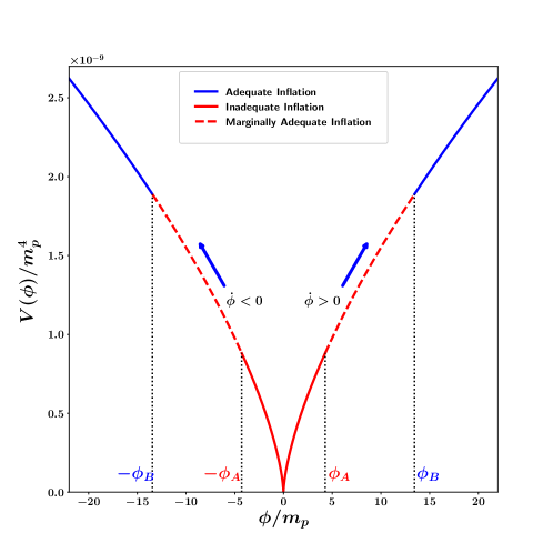
Figure 10: This figure schematically shows initial field values which result in adequate inflation with $N_{e}\geq 60$ (blue), marginally adequate (dashed red) and inadequate inflation (red) for the monodromy potential (28). The initial energy scale is $H_{i}=3\times 10^{-3}m_{p}$. As earlier, blue lines represent regions of adequate inflation. The red lines come in two styles: dashed/solid and correspond to the two possible initial directions of ${\dot{\phi}}$. The solid red line represents initial values of $\phi$ for which inflation is never adequate irrespective of the direction of ${\dot{\phi}_{i}}$. In the region shown by the dashed red line one gets adequate inflation only when ${\dot{\phi}_{i}}$ points in the direction (shown by blue arrows) of increasing $V(\phi)$. Note that only a small portion of the full potential is shown in this figure.

Initial values of $\phi$ that lead to adequate or inadequate inflation are schematically shown in figure 10. Inadequate inflation arises when the scalar field originates in the region $\phi_{i}\in[-\phi_{A},\phi_{A}]$, shown by solid red lines. Blue lines represent initial field values $\phi_{i}\in\big{(}-\phi_{m},-\phi_{B}\big{)}\cup\big{(}\phi_{B},\phi_{m}\big{)}$, which always result in adequate inflation. Note that $\phi_{m}$ is the maximum allowed value of $\phi$ for a given initial energy scale, as determined from the consistency equations (14), (20). The initial conditions $\phi_{i}\in\big{[}-\phi_{B},-\phi_{A}\big{]}\cup\big{[}\phi_{A},\phi_{B}\big{]}$, shown by dashed red lines, lead to adequate inflation only when ${\dot{\phi}}_{i}$ points in the direction (shown by blue arrows) of increasing $V(\phi)$. We refer to this as marginally adequate inflation. The dependence of $\phi_{A}$ and $\phi_{B}$ on the initial energy scale $H_{i}$ is shown in Table 3.

As in the case of chaotic inflation, we determine the fraction of initial conditions that do not lead to adequate inflation (the degree of inadequate inflation), by assuming a uniform distribution of initial values of $Y=\dot{\phi}$ and $X=\hat{\phi}\sqrt{2V(\phi)}$ on the circular boundary (14), (20) with $V(\phi)$ given by (28). Our results are given in table 3. As was the case for quadratic chaotic inflation, we once more find that $\frac{\Delta l_{A}}{l}$ and $\frac{\Delta l_{B}}{l}$ decrease with an increase in $H_{i}$; see table 3, figures 11 and 11.

$H_{i}$ (in $m_{p}$)	$\phi_{A}$ (in $m_{p}$)	$\phi_{B}$ (in $m_{p}$)	$2\frac{\Delta l_{A}}{l}$	$2\frac{\Delta l_{B}}{l}$
$3\times 10^{-3}$	$4.29$	$13.45$	$3.64\times 10^{-3}$	$5.33\times 10^{-3}$
$3\times 10^{-2}$	$2.41$	$15.33$	$3.0\times 10^{-4}$	$5.56\times 10^{-4}$
$3\times 10^{-1}$	$0.61$	$17.22$	$2.08\times 10^{-5}$	$5.78\times 10^{-5}$

Table 3: Dependence of $\phi_{A}$, $\phi_{B}$, $\frac{\Delta l_{A}}{l}$ and $\frac{\Delta l_{B}}{l}$ on the initial energy scale $H_{i}$ for monodromy inflation with $p=\frac{2}{3}$. Here $l=2\pi R\equiv 2\pi\sqrt{6}H_{i}/m_{p}$ and $\frac{\Delta l_{A}}{l}$, $\frac{\Delta l_{B}}{l}$ were defined in figure 4. Note that the fraction of initial conditions which leads to inadequate inflation, $2\frac{\Delta l_{A}}{l}$, decreases as $H_{i}$ is increased. The same is true for the fraction of initial conditions giving rise to marginally adequate inflation, $2\frac{\Delta l_{B}}{l}$. The fraction of initial conditions leading to adequate inflation, with $N_{e}\geq 60$, is given by $1-2\frac{\Delta l_{B}}{l}$. Thus inflation proves to be more general for larger values of the initial energy scale $H_{i}$, since a larger initial region in phase space gives rise to adequate inflation with $N_{e}\geq 60$.

III.3 Comparison of power law potentials

In this subsection we compare the generality of inflation for the power law family of potentials, $V\propto|\phi|^{p}$, by plotting the fraction of initial conditions that do not lead to adequate inflation ($2\frac{\Delta l_{A}}{l}$ and $2\frac{\Delta l_{B}}{l}$) in figures 11 and 11; also see tables 1-3. These figures demonstrate that the set of initial conditions which give rise to adequate inflation (with $N_{e}\geq 60$) increases with the energy scale of inflation, $H_{i}$. We also find that inflation is sourced by a larger set of initial conditions for the monodromy potential $V\propto|\phi|^{\frac{2}{3}}$, which is followed by $V\propto|\phi|$ and $V\propto\phi^{2}$ respectively. Finally we draw attention to the fact that our conclusions remain unchanged if we determine the degree of inflation by a different measure such as $\frac{\Delta\phi_{A}}{\phi_{max}}$ and $\frac{\Delta\phi_{B}}{\phi_{max}}$, where $\phi_{max}$ is the maximum allowed value of $\phi$ for a given inflationary energy scale.

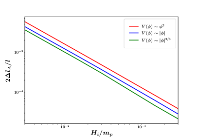
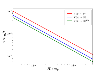
Figure 11: This figure shows the fraction of initial conditions that leads to (a) inadequate inflation, $2\frac{\Delta l_{A}}{l}$ and (b) marginally adequate inflation, $2\frac{\Delta l_{B}}{l}$, plotted against the initial energy scale of inflation, $H_{i}$. For the definition of $\frac{\Delta l_{A}}{l}$ and $\frac{\Delta l_{B}}{l}$, see figure 4. The red curve shows results for $V\propto\phi^{2}$ while the blue and green curves represent monodromy potentials with $V\propto|\phi|,|\phi|^{2/3}$ respectively. The decrease in $2\frac{\Delta l_{A}}{l}$ and $2\frac{\Delta l_{B}}{l}$, which accompanies an increase in $H_{i}$ is indicative of the fact that the set of initial conditions which give rise to adequate inflation (with $N_{e}\geq 60$) increases with the energy scale of inflation, $H_{i}$. This figure also demonstrates that inflation is sourced by a larger set of initial conditions for the monodromy potential $V\propto|\phi|^{\frac{2}{3}}$, which is followed by $V\propto|\phi|$ and finally $V\propto\phi^{2}$.

IV Higgs Inflation

It would undoubtedly be interesting if inflation could be realized within the context of the Standard Model ($SM$) of particle physics. Since the $SM$ has only a single scalar degree of freedom, namely the Higgs field, one can ask whether the Higgs field (30) can source inflation. Unfortunately the self-interaction coupling of the Higgs field, $\lambda$ in (30), is far too large to be consistent with the small amplitude of scalar fluctuations observed by the cosmic microwave background CMB .

This situation can however be remedied if either of the following possibilties is realized: (i) the Higgs couples non-minimally to gravity, or (ii) the Higgs field is described by a non-canonical Lagrangian

Indeed, as first demonstrated in higgs1 , inflation can be sourced by the $SM$ Higgs potential if the Higgs field is assumed to couple non-minimally to the Ricci scalar. The resultant inflationary model provides a good fit to observations and has been extensively developed and examined in higgs1 ; higgs2 ; higgs3 ; higgs4 ; higgs5 . A different means of sourcing Inflation through the Higgs field was discussed in sanil_varun where it was shown that the $SM$ Higgs potential with a non-canonical kinetic term fits the CMB data very well by accounting for the currently observed values of the scalar spectral index $n_{{}_{S}}$ and the tensor-to-scalar ratio $r$. We shall proceed to study Higgs inflation first in the non-minimal framework in section IV.1 followed by the same in the non-canonical framework in section IV.2.

IV.1 Initial conditions for Higgs Inflation in the non-minimal framework

Inflation sourced by the Standard Model ($SM$) Higgs boson was first discussed in higgs1 . In this model the Higgs non-minimally couples to gravity with a moderate value of the non-minimal coupling higgs2 ; higgs3 . The model does not require an additional degree of freedom beyond the $SM$ and fits the observational data quite well CMB . Reheating after inflation in this model has been studied in detail higgs3 ; higgs4 ; higgs4a and quantum corrections to the potential at very high energies have been shown to be small higgs5 . In this section we assess the generality of Higgs inflation (in the Einstein frame) and determine the range of initial conditions which gives rise to adequate inflation (with $N_{e}\geq 60$) for a given value of the initial energy scale.

Action for Higgs Inflation

The action for a scalar field $\phi$ which couples non-minimally to gravity (i.e.  in the Jordan frame) is given by higgs1 ; higgs2 ; kaiser

$$S_{J}=\int d^{4}x\sqrt{-g}\bigg{[}f(\phi)R-\frac{1}{2}g^{\mu\nu}\partial_{\mu}\phi\partial_{\nu}\phi-U(\phi)\bigg{]}$$ (29)

where $R$ is the Ricci scalar and $g_{\mu\nu}$ is the metric in the Jordan frame. The potential for the $SM$ Higgs field is given by

$$U(\phi)=\frac{\lambda}{4}\Big{(}\phi^{2}-\sigma^{2}\Big{)}^{2}$$ (30)

where $\sigma$ is the vacuum expectation value of the Higgs field

$$\sigma=246\,GeV=1.1\times 10^{-16}m_{p}$$ (31)

and the Higgs coupling constant has the value $\lambda=0.1$. Furthermore

$$f(\phi)=\frac{1}{2}(m^{2}+\xi\phi^{2})$$ (32)

where $m$ is a mass parameter given by kaiser

$$m^{2}=m_{p}^{2}-\xi\sigma^{2}$$

$\xi$ being the non-minimal coupling constant whose value

$$\xi=1.62\times 10^{4}$$ (33)

agrees with observations CMB (see Appendix A). For the above values of $\sigma$ and $\xi$, one finds $m\simeq m_{p}$, so that

$$f(\phi)\simeq\frac{1}{2}(m_{p}^{2}+\xi\phi^{2})=\frac{m_{p}^{2}}{2}\Big{(}1+\frac{\xi\phi^{2}}{m_{p}^{2}}\Big{)}~{}.$$ (34)

We now transfer to the Einstein frame by means of the following conformal transformation of the metric kaiser

$$g_{{\mu}{\nu}}\longrightarrow\hat{g}_{{\mu}{\nu}}=\Omega^{2}g_{{\mu}{\nu}}$$ (35)

where the conformal factor is given by

$$\Omega^{2}=\frac{2}{m_{p}^{2}}f(\phi)=1+\frac{\xi\phi^{2}}{m_{p}^{2}}~{}.$$ (36)

After the field redefinition $\phi\longrightarrow\chi$ the action in the Einstein frame is given by kaiser

$$S_{E}=\int d^{4}x\sqrt{-\hat{g}}\bigg{[}\frac{m_{p}^{2}}{2}\hat{R}-\frac{1}{2}\hat{g}^{\mu\nu}\partial_{\mu}\chi\partial_{\nu}\chi-V(\chi)\bigg{]}$$ (37)

where

$$V(\chi)=\frac{U[\phi(\chi)]}{\Omega^{4}}$$ (38)

and

$$\frac{\partial\chi}{\partial\phi}=\pm\frac{1}{\Omega^{2}}\sqrt{\Omega^{2}+\frac{6\xi^{2}\phi^{2}}{m_{p}^{2}}}~{}.$$ (39)

Eq. (37) describes General Relativity (GR) in the presence of a minimally coupled scalar field $\chi$ with the potential $V(\chi)$. (The full derivation of the action in the Einstein frame is given in appendix B.)

Limiting cases of the potential in the Einstein Frame

From equations (36) and (39) one finds the following asymptotic forms for the potential (38) (for details see appendix C and higgs1 ; higgs3 )

1. For $\phi\ll\sqrt{\frac{2}{3}}\frac{m_{p}}{\xi}$ one finds

   $$\chi=\pm\phi,~{}~{}~{}~{}V(\chi)\simeq\frac{\lambda}{4}\chi^{4},~{}~{}~{}~{}|\chi|\ll\sqrt{\frac{2}{3}}\frac{m_{p}}{\xi}.$$ (40)

2. For $\sqrt{\frac{2}{3}}\frac{m_{p}}{\xi}\ll\phi\ll\frac{m_{p}}{\sqrt{\xi}}$,

   $$\chi=\pm\sqrt{\frac{3}{2}}\frac{\xi\phi^{2}}{m_{p}},~{}~{}~{}~{}V(\chi)\simeq\left(\frac{\lambda m_{p}^{2}}{6\xi^{2}}\right)\chi^{2},~{}~{}~{}~{}\sqrt{\frac{2}{3}}\frac{m_{p}}{\xi}\ll|\chi|\ll\sqrt{\frac{3}{2}}m_{p}.$$ (41)

3. For $\phi\gg\frac{m_{p}}{\sqrt{\xi}}$

   $$\chi=\pm\sqrt{6}m_{p}\log{\left(\frac{\sqrt{\xi}\phi}{m_{p}}\right)},~{}~{}~{}V(\chi)\simeq\frac{\frac{\lambda m_{p}^{4}}{4\xi^{2}}}{\left(1+\exp\Big{[}-\sqrt{\frac{2}{3}}\frac{|\chi|}{m_{p}}\Big{]}\right)^{2}},~{}~{}~{}~{}|\chi|\gg\sqrt{\frac{3}{2}}m_{p}$$ (42)

A good analytical approximation to the potential which can accommodate both (41) and (42) is

$$V(\chi)\simeq V_{0}\left(1-\exp\Big{[}-\sqrt{\frac{2}{3}}\frac{|\chi|}{m_{p}}\Big{]}\right)^{2},~{}~{}~{}~{}|\chi|\gg\sqrt{\frac{2}{3}}\frac{m_{p}}{\xi}$$ (43)

where $V_{0}$ is given by (Appendix A)

$$V_{0}=\frac{\lambda m_{p}^{4}}{4\xi^{2}}=9.6\times 10^{-11}~{}m_{p}^{4}~{}.$$ (44)

Generality Analysis of Higgs inflation in the Einstein Frame

As we have seen, Higgs inflation in the Einstein frame can be described by a minimally coupled canonical scalar field $\chi$ with a suitable potential $V(\chi)$. We have analysed two different limits of the potential $V(\chi)$ which is asymptotically flat and has plateau like arms for $|\chi|\gg 1$. One notes that when $|\chi|\to 0$, $V(\chi)$ has a tiny kink with amplitude $\frac{\lambda}{4}\sigma^{4}\sim 10^{-66}m_{p}^{4}$. This kink is much smaller than the maximum height of the potential and can be neglected for all practical purposes. (This is simply a reflection of the fact that the inflation energy scale is much larger than the electro-weak scale.) We have numerically evaluated the potential defined in (38) & (39) and compared it with the approximate form given in equation (43); see figure 12. The difference between the two potentials is shown in figure 13. One finds that the maximum fractional difference between the two potentials is only $0.16\%$ which justifies the use of (43) for further analysis.

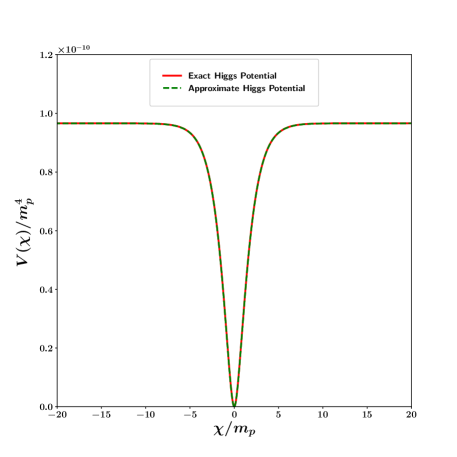
Figure 12: This figure shows the potential for Higgs inflation (in the Einstein frame) in units of $m_{p}^{4}$. The (solid) red curve shows the numerically determined value of the potential from (38) & (39), while the (dashed) green curve shows the approximate potential $V(\chi)=V_{0}\left(1-\exp{[-\sqrt{\frac{2}{3}}\frac{|\chi|}{m_{p}}]}\right)^{2}$. Clearly the approximate form matches the exact one very well.

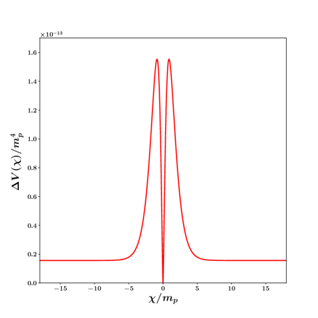
Figure 13: This figure shows the absolute value of the difference between the numerically determined Higgs potential (38) & (39), and the approximate form (43). We see that the maximum difference is near $\chi\sim m_{p}$ and its fractional value is only $0.16\%$.

During Higgs inflation, the slow-roll parameter is given by

$$\epsilon=\frac{m_{p}^{2}}{2}\left(\frac{1}{V}\frac{dV}{d\chi}\right)^{2}=\frac{4}{3}\frac{1}{\left(\exp\left(\sqrt{\frac{2}{3}}\frac{|\chi|}{m_{p}}\right)-1\right)^{2}}~{},$$ (45)

since slow-roll ends when $\epsilon\simeq 1$, one finds

$$|\chi|\simeq 0.94~{}m_{p}\sim m_{p}~{}.$$

We study the generality of Higgs inflation in the Einstein frame by plotting the phase-space diagram for the potential (43) and determining the region of initial conditions which lead to adequate inflation (i.e.  $N_{e}\geq 60$). Our results are shown in figure 14 and a zoomed-in view is presented in figure 15.

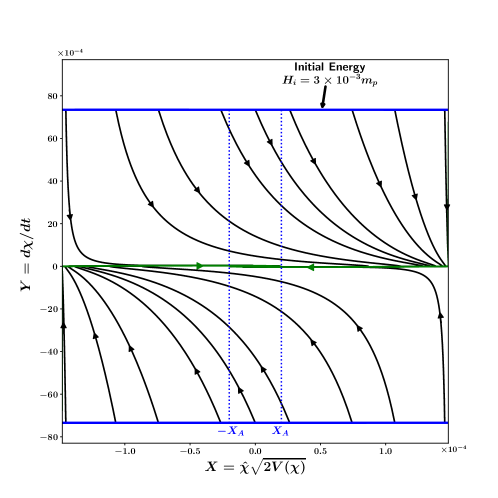
Figure 14: This figure shows the phase-space of Higgs inflation in the Einstein frame. $Y=d\chi/dt$ is plotted against $X=\hat{\chi}\sqrt{2V(\chi)}$ for the initial energy scale $H_{i}=3\times 10^{-3}m_{p}$. ($\hat{\chi}=\frac{\chi}{|\chi|}$ is the sign of field $\chi$.) We see that commencing from a fixed initial energy (shown by the blue boundary lines), most solutions rapidly converge towards the two inflationary separatrices (horizontal green lines) corresponding to slow-roll inflation. We therefore find that inflation for the Higgs potential is remarkably general and can commence from a very wide class of initial conditions. Note that trajectories lying close to the origin, i.e.  within the vertical band marked by $(-X_{A},X_{A})$, are strongly curved. This property allows them to converge to the inflationary separatrices giving rise to adequate inflation with $N_{e}\geq 60$. It is interesting to contrast this behaviour with that of chaotic inflation, shown in figure 1, for which there is a small region with inadequate inflation near the center. Because of this property, the Higgs scenario displays adequate inflation over a slightly larger range of initial conditions when compared with chaotic inflation.

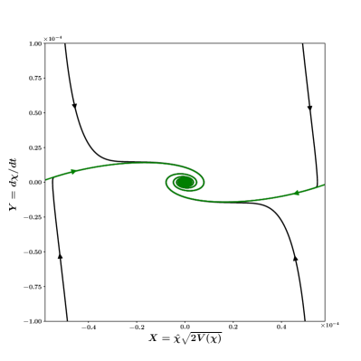
Figure 15: A zoomed-in view of the central region in figure 14. We see that most trajectories (associated with different initial conditions) initially converge towards the horizontal slow-roll inflationary separatrics (green lines) before spiralling in towards the center. (The spiral reflects oscillations of the inflaton about the minimum of its potential.)

We see that the phase-space diagram for Higgs inflation has very interesting properties. The asymptotically flat arms result in robust inflation as expected. However it is also possible to obtain adequate inflation if the inflaton commences from $\chi\simeq 0$. This is because the scalar field is able to climb up the flat wings of $V(\chi)$. This property is illustrated in figure 14 by lines originating in the central region, which are slanted and hence can converge to the slow-roll inflationary separatrics resulting in adequate inflation. This feature is not shared by chaotic inflation where one cannot obtain adequate inflation by starting from the origin (provided the initial energy scale is not too large, i.e.  $H_{i}<m_{p}$.)

This does not however imply that all possible initial conditions lead to adequate inflation in the Higgs scenario. As shown in figure 16 there is a small region of initial field values denoted by $|\chi_{A}|<|\chi_{i}|<|\chi_{B}|$ which does not lead to adequate inflation if $\chi_{i}$ and $\dot{\chi_{i}}$ have opposite signs (dashed red lines). By contrast, the solid blue lines in the same figure show the region of $\chi_{i}$ that results in adequate inflation independently of the direction of the initial velocity $\dot{\chi_{i}}$. The dependence of $\chi_{A}$ and $\chi_{B}$ on the initial energy scale is shown in table 4 (also see figure 16). Note the surprising fact that the value of $\chi_{B}-\chi_{A}$ remains virtually unchanged as $H_{i}$ increases.

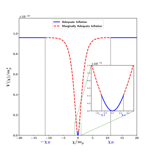
Figure 16: This figure shows initial field values, $\chi_{i}$, which either lead to adequate inflation (solid blue lines) or partially adequate inflation (dashed red lines). The region corresponding to $\chi_{i}\in[-\chi_{B},-\chi_{A}]\cup[\chi_{A},\chi_{B}]$ (dashed red) leads to partially adequate inflation. Initial field values originating in this region result in inadequate inflation only when $\dot{\chi_{i}}$ is directed towards decreasing values of $V(\chi)$. The alternative case, with $\dot{\chi_{i}}$ directed towards increasing $V(\chi)$, leads to adequate inflation for the same subset $\chi_{i}\in[-\chi_{B},-\chi_{A}]\cup[\chi_{A},\chi_{B}]$. This figure is shown for an initial energy scale $H_{i}=3\times 10^{-3}m_{p}$. The precise values of $\chi_{A}$ and $\chi_{B}$ depend on the initial energy scale $H_{i}$ as shown in table 4. Note that only a small portion of the full potential is shown in this figure.

$H_{i}$ (in $m_{p}$)	$\chi_{A}$ (in $m_{p}$)	$\chi_{B}$ (in $m_{p}$)	$\chi_{B}-\chi_{A}$ (in $m_{p}$)
$3\times 10^{-3}$	$0.28$	$11.11$	$10.83$
$3\times 10^{-2}$	$2.16$	$12.99$	$10.83$
$3\times 10^{-1}$	$4.04$	$14.87$	$10.83$

Table 4: Dependence of $\chi_{A}$ and $\chi_{B}$ on the initial energy scale $H_{i}$ for Higgs inflation (also see figure 16).

The results of figures 14, 15 and 16 lead us to conclude that there is a region lying close to the origin of $V(\chi)$, namely $\chi_{i}\in(-\chi_{A},\chi_{A})$, where one gets adequate inflation regardless of the direction of $\dot{\chi}_{i}$. One might note that this feature is absent in the power law family of potentials described in the previous section (compare figure 16 with figures 3, 7, 10). values that lead to partially adequate inflation, $|\chi_{i}|\in[|\chi_{A}|,|\chi_{B}|]$ We therefore conclude that a wide range of initial conditions can generate adequate inflation in the Higgs case, which does not support some of the conclusions drawn in stein13 .

Finally we would like to draw attention to the fact that the phase-space analysis performed here for Higgs inflation is likely to carry over to the T-model $\alpha$-attractor potential T-model , since the two potentials are qualitatively very similar.

IV.2 Initial conditions for Higgs Inflation in the non-canonical framework

The class of initial conditions leading to sufficient inflation widens considerably if we choose to work with scalar fields possessing a non-canonical kinetic term.

The Lagrangian for this class of models is Mukhanov-2006

$${\cal L}(\phi,F)=-F\left(\frac{F}{M^{4}}\right)^{\alpha-1}-V(\phi),$$ (46)

where $F=\frac{1}{2}\partial_{\mu}\phi\;\partial^{\mu}\phi$, $M$ has the dimensions of mass and $\alpha$ is a dimensionless parameter. The associated energy density and pressure in a FRW universe are given by Mukhanov-2006 ; sanil_varun

$$\rho_{\phi}=-(2\alpha-1)F\left(\frac{F}{M^{4}}\right)^{\alpha-1}+V(\phi)~{},$$ (47)

$$p_{\phi}=-F\left(\frac{F}{M^{4}}\right)^{\alpha-1}-V(\phi)~{},~{}~{}F=-\frac{1}{2}{\dot{\phi}}^{2}~{},$$ (48)

which reduce to the canonical form $\rho_{\phi}=-F+V,~{}p_{\phi}=-F-V$ when $\alpha=1$. The two Friedmann equations now acquire the form

$$H^{2} = \frac{8\pi G}{3}\left[-(2\alpha-1)F\left(\frac{F}{M^{4}}\right)^{\alpha-1}+\;V(\phi)\right]~{},$$ (49)

$$\frac{\ddot{a}}{a} = -\frac{8\pi G}{3}\left[-(\alpha+1)F\left(\frac{F}{M^{4}}\right)^{\alpha-1}-\;V(\phi)\right]~{},$$ (50)

and the equation of motion of the scalar field becomes

$$\ddot{\phi}+\frac{3}{2\alpha-1}H\dot{\phi}+\left(\frac{V^{\prime}(\phi)}{\alpha(2\alpha-1)}\right)\left(\frac{2M^{4}}{\dot{\phi}^{2}}\right)^{\alpha-1}=0,$$ (51)

which reduces to (16) when $\alpha=1$.

Before discussing Higgs inflation in the non-canonical framework, we first examine the inflationary slow-roll parameter $\epsilon_{nc}$ which, for non-canonical inflation, is given by sanil_varun

$$\epsilon_{nc}=\left(\frac{1}{\alpha}\right)^{\frac{1}{2\alpha-1}}\left(\frac{3M^{4}}{V}\right)^{\frac{\alpha-1}{2\alpha-1}}\left(\epsilon_{c}\right)^{\frac{\alpha}{2\alpha-1}},$$ (52)

$\epsilon_{c}$ being the canonical slow-roll parameter (18). Note that $\epsilon_{nc}<\epsilon_{c}$ for $3M^{4}\ll V$. This suggests that for a fixed potential $V$, the duration of inflation can be enhanced relative to the canonical case ($\alpha=1$), by a suitable choice of $M$.

The Higgs potential

It is well known that the standard model Higgs boson, when coupled minimally to gravity, cannot provide a working model of inflation due to the large value of the coupling constant, $\lambda\simeq 0.1$, in the potential

$$V(\phi)=\frac{\lambda}{4}\left(\phi^{2}-\sigma^{2}\right)^{2},$$ (53)

where $\sigma$ is the vacuum expectation value of the Higgs field (31). Indeed $\lambda\simeq 0.1$ is many orders of magnitude larger than the CMB constrained value $\lambda_{c}\simeq 1.43\times 10^{-13}$ in the canonical framework (see Appendix A). Additionally the potential (53) gives too small a value for the inflationary scalar spectral index $n_{{}_{S}}$ and too large a value for the tensor-to-scalar ratio $r$, to be in accord with observations.

However the situation changes when one examines the potential (53) in the non-canonical framework. The expression for the inflationary scalar spectral index now becomes sanil_varun

$$n_{{}_{S}}=1-\left(\frac{\gamma+4}{N_{e}\gamma+2}\right)~{},$$ (54)

where

$$\gamma\equiv\frac{2(3\alpha-2)}{2\alpha-1}~{}.$$ (55)

Since $\gamma$ increases from $\gamma=2$ for $\alpha=1$ to $\gamma=3$ for $\alpha\gg 1$, therefore the scalar spectral index increases from the canonical value $n_{{}_{S}}=0.951$ ($\alpha=1,N_{e}=60$) to $n_{{}_{S}}=0.962$, in non-canonical models (with $\alpha\gg 1$).

Similarly one can show that the tensor-to-scalar ratio declines in non-canonical models. For the Higgs potential one gets sanil_varun

$$r=\left(\frac{1}{\sqrt{2\,\alpha-1}}\right)\left(\frac{32}{N_{e}\gamma+2}\right)~{},$$ (56)

which demonstrates that the value of $r$ decreases with an increase in the non-canonical parameter $\alpha$. Figure 17 shows $n_{{}_{S}}$, $r$ plotted as functions of $\alpha$. One finds that $n_{{}_{S}}\simeq 0.96$, $r<0.1$ for $\alpha\geq 3$, which agrees well with CMB observations.

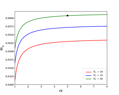
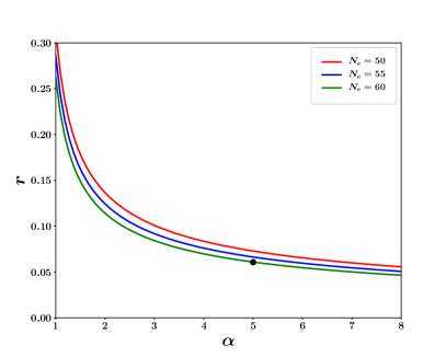
Figure 17: This figure shows: (a) the scalar spectral index $n_{{}_{S}}$, (b) the tensor to scalar ratio $r$, as functions of the non-canonical parameter $\alpha$ and described respectively by equations (54) and (56). Three values of the number of e-foldings, $N_{e}=50,~{}55$ and $60$, are chosen. One finds that larger values of $\alpha$ result in higher values of $n_{{}_{S}}$ and lower values of $r$. The black dot in both figures indicates the value of $\alpha$, and the corresponding values of $n_{{}_{S}}$ and $r$, used in our subsequent analysis.

The relation between the value of the Higgs self-coupling $\lambda\simeq 0.1$ in the non-canonical framework and the corresponding canonical value $\lambda_{c}$ is given by sanil_varun

$$\lambda=4\left[\frac{32\lambda_{c}(N_{e}+1)^{3}}{\sqrt{2\alpha-1}}\left(\frac{\alpha}{4}\Big{(}\frac{1}{6}\frac{m_{p}^{4}}{M^{4}}\Big{)}^{\alpha-1}\right)^{\frac{2}{3\alpha-2}}\left(\frac{1}{N_{e}\gamma+2}\right)^{\frac{\gamma+4}{\gamma}}\right]^{\frac{3\alpha-2}{\alpha}}~{},$$ (57)

where consistency with CMB observations suggests $\lambda_{c}\sim 10^{-13}$.

Figure 18 describes the values of the non-canonical parameters $\alpha$ and $M$ that yield $\lambda\simeq 0.1$ in (53) – the relation between $M$ and $\alpha$ being provided by equation (57). In our subsequent analysis we choose $\alpha=5$ for simplicity. This is shown by the black color dot in figure 17 and 17. (The corresponding value of $M$ is shown by the green dot in figure 18.)

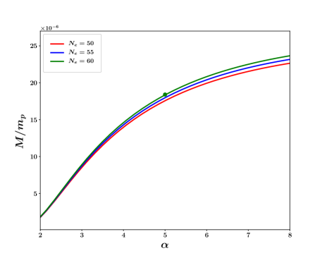
Figure 18: This figure illustrates the relation between the non-canonical parameters $M$ and $\alpha$, given by equation (57), which results in the self-coupling value $\lambda=0.1$ in equation (53). Results for three different e-folding values $N_{e}=50,~{}55~{},60$ are shown. The green dot indicates the value of $M$ and $\alpha$ which is used in our subsequent analysis.

As in the case of canonical scalar fields (20), one can rewrite the Friedman equation for non-canonical scalars (49) as follows

$$R^{2}=Y_{nc}^{2}+X^{2}$$ (58)

where

$$R=\sqrt{6}\frac{H}{m_{p}},~{}~{}X=\hat{\phi}\frac{\sqrt{2V(\phi)}}{m_{p}^{2}},~{}~{}Y_{nc}=\left[2(2\alpha-1)\left(-\frac{F}{m_{p}^{4}}\right)\left(\frac{F}{M^{4}}\right)^{\alpha-1}\right]^{1/2}.$$ (59)

Therefore commencing at some initial value of $R$ ($\equiv\sqrt{6}H/m_{p}$) one can set different initial conditions by varying $X$ and $Y_{nc}$. Since $X$, $Y_{nc}$ satisfy the constraint equation (58) they lie on the boundary of a circle.

We probe the robustness of this model to initial conditions by plotting its phase-space diagram ($Y_{nc}$ vs $X$) and determining the region of initial conditions which gives rise to adequate inflation ($N_{e}\geq 60$) for values of $M$ and $\alpha$ which satisfy CMB constraints (shown by the green dot in figure 18). The phase-space diagram corresponding to an initial energy scale $H_{i}=3\times 10^{-3}~{}m_{p}$ is shown in figure 19.

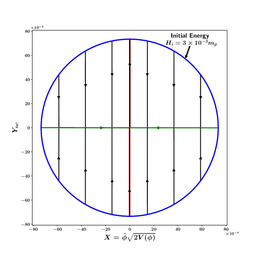
Figure 19: This figure shows the phase-space of Higgs inflation in the non-canonical framework described by (53). $Y_{nc}$, given by (59) is plotted against $X$ ($=\hat{\phi}\sqrt{2V(\phi)}$) for different initial conditions all of which commence on the (blue) circle which represents the initial energy scale $H_{i}=3\times 10^{-3}m_{p}$. ($\hat{\phi}=\frac{\phi}{|\phi|}$ is the sign of field $\phi$.) One finds that commencing from the circle, different inflationary trajectories rapidly converge to one of the two inflationary separatrices (green horizontal lines) before proceeding towards the center, which corresponds to the minimum of the potential. The thin vertical central red band corresponds to the region in phase-space that does not lead to adequate inflation. Note that this band is very small which is indicative of the robustness of Higgs inflation in the non-canonical framework. The arc-length of the red band, when divided by the circumference of the circle with radius = $\sqrt{6}H_{i}/m_{p}$, gives the fraction of initial conditions $\frac{2\Delta l_{A}}{l}$ which lead to inadequate inflation.

The fraction of initial conditions which give rise to inadequate inflation, $\frac{2\Delta l_{A}}{l}$, and partially adequate inflation, $\frac{2\Delta l_{B}}{l}$, are shown in table 5. (As earlier, a uniform distribution of $X$ and $Y_{nc}$ on the boundary of initial conditions has been assumed.) From this table one finds that the values of $\phi_{A}$ and $\phi_{B}$ associated with an initial energy scale $H_{i}$, are much smaller than their counterparts for canonical inflation (see figures 20, 20 and 21). This is a consequence of the fact that for identical potentials, the slow-roll parameter in the non-canonical case is much smaller than its canonical counterpart ($\epsilon_{nc}\ll\epsilon_{c}$), which permits inflation to commence from smaller values of the inflaton field in the non-canonical case. We also find that the fraction of non-inflationary initial conditions, $\frac{\Delta l_{A}}{l}$, decreases with an increase $H_{i}$, as expected.

$H_{i}$ (in $m_{p}$)	$\phi_{A}$ (in $m_{p}$)	$\phi_{B}$ (in $m_{p}$)	$2\frac{\Delta l_{A}}{l}$	$2\frac{\Delta l_{B}}{l}$
$3\times 10^{-3}$	$8.74\times 10^{-3}$	$9.07\times 10^{-3}$	$1.48\times 10^{-3}$	$1.59\times 10^{-3}$
$3\times 10^{-2}$	$8.66\times 10^{-3}$	$8.99\times 10^{-3}$	$1.45\times 10^{-4}$	$1.57\times 10^{-4}$
$3\times 10^{-1}$	$8.58\times 10^{-3}$	$8.91\times 10^{-3}$	$1.43\times 10^{-5}$	$1.54\times 10^{-5}$

Table 5: Dependence of $\phi_{A}$, $\phi_{B}$, $\frac{\Delta l_{A}}{l}$ and $\frac{\Delta l_{B}}{l}$ on the initial energy scale $H_{i}$ for non-canonical Higgs inflation . Here $l=2\pi R\equiv 2\pi\sqrt{6}H_{i}/m_{p}$.

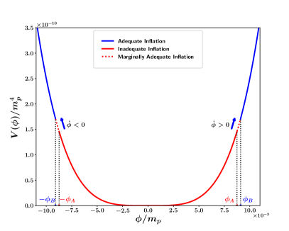
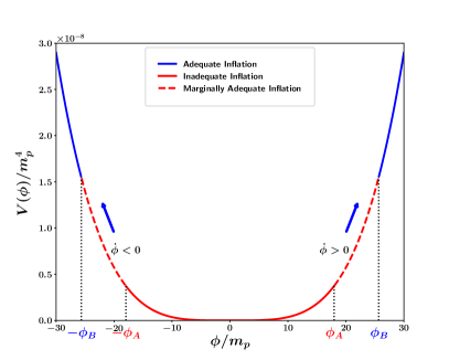
Figure 20: Initial field values, $\phi_{i}$, which lead to adequate inflation with $N_{e}\geq 60$ (blue), marginally adequate (dashed red) and inadequate (red) inflation are schematically shown for the Higgs inflation with the quartic potential (53): (a) in the non-canonical framework and (b) in the canonical framework. The blue lines represent regions of adequate inflation. The red lines come in two styles: dashed/solid and correspond to the two possible initial directions of ${\dot{\phi}_{i}}$. The solid red line represents initial values of $\phi$ for which inflation is never adequate irrespective of the direction of ${\dot{\phi}_{i}}$. In the region shown by the dashed line one gets adequate inflation only when ${\dot{\phi}_{i}}$ points in the direction of increasing $V(\phi)$. We note that for the non-canonical case, the values of $\phi_{A}$ and $\phi_{B}$ are extremely small as shown in table 5. (Only a small portion of the full potential is shown in this figure which corresponds to the initial energy scale $H_{i}=3\times 10^{-3}m_{p}$.)

In figure 21 we compare values of $\frac{\Delta l_{A}}{l}$ and $\frac{\Delta l_{B}}{l}$ for canonical inflation with $V_{c}(\phi)=\frac{\lambda_{c}}{4}\phi^{4}$ and non-canonical inflation with $V(\phi)=\frac{\lambda}{4}\phi^{4}$ where $\lambda$ and $\lambda_{c}$ are related by equation (57). We find that the values of $\frac{\Delta l_{A}}{l}$ and $\frac{\Delta l_{B}}{l}$ are significantly smaller for non-canonical inflation, which implies that inflation arises from a larger class of initial conditions in the non-canonical framework.

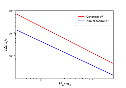
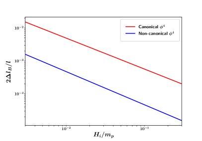
Figure 21: This figure compares the values of (a) $\frac{\Delta l_{A}}{l}$ and (b) $\frac{\Delta l_{B}}{l}$ for canonical and non-canonical scalar fields with the potential $V(\phi)\propto\phi^{4}$. $\frac{\Delta l_{A}}{l}$ and $\frac{\Delta l_{B}}{l}$ are shown as functions of the initial energy scale of inflation, $H_{i}$. The red and blue curves correspond to canonical and non-canonical quartic inflation respectively. The smaller amplitude of the blue curve in both panels indicates that non-canonical inflation arises for a larger class of initial conditions than canonical inflation (red). The decrease in $\frac{\Delta l_{A}}{l}$ and $\frac{\Delta l_{B}}{l}$ with an increase in $H_{i}$ is indicative of the fact that the set of initial conditions which give rise to adequate inflation (with $N_{e}\geq 60$) increases with the energy scale of inflation, $H_{i}$.

V Starobinsky Inflation

V.1 Action and Potential in the Einstein Frame

Starobinsky inflation star80 is based on the action

$$S=\int d^{4}x\sqrt{-g}\frac{m_{p}^{2}}{2}\bigg{[}R+\frac{1}{6m^{2}}R^{2}\bigg{]}~{},$$ (60)

where $m$ is a mass parameter. The corresponding action in the Einstein frame is given by whitt84 ; maeda88 ; gorbunov13

$$S_{E}=\int d^{4}x\sqrt{-g}\bigg{[}\frac{m_{p}^{2}}{2}\hat{R}-\frac{1}{2}\hat{g}^{\mu\nu}\partial_{\mu}\phi\partial_{\nu}\phi-V(\phi)\bigg{]}$$ (61)

where the inflaton potential is

$$V(\phi)=\frac{3}{4}m^{2}m_{p}^{2}\Big{(}1-e^{-\sqrt{\frac{2}{3}}\frac{\phi}{m_{p}}}\Big{)}^{2}$$ (62)

and $m=1.13\times 10^{-5}m_{p}$ is required from an analysis of scalar fluctuations gorbunov13 (see Appendix A). The potential (62) is shown in figure 22.

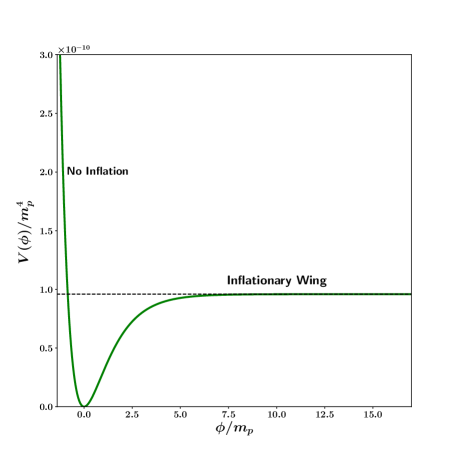
Figure 22: The effective potential in Starobinsky Inflation, (62), is plotted in units of $m_{p}^{4}$. The potential is asymmetric about the origin and has a steep left wing and plateau-like right wing. Inflation occurs along the flat plateau-like right wing, the steep left wing being unable to sustain inflation.

As shown in figure 22, the potential for Starobinsky inflation is asymmetric about the origin. One should note that the flat right wing of the potential has the same functional form as the Higgs inflation potential in the Einstein frame. However the left wing of $V(\phi)$ is very steep. The slow-roll parameter for this potential is given by

$$\epsilon=\frac{4}{3}\left[\exp\left(\sqrt{\frac{2}{3}}\frac{\phi}{m_{p}}\right)-1\right]^{-2}.$$

Inflation occurs for $\epsilon\leq 1$, which corresponds to $\phi\geq 0.94~{}m_{p}$ and implies that no inflation can happen on the steep left wing of the potential (for which $\phi<0$).

V.2 Generality of Starobinsky Inflation

The distinctive properties of the Starobinsky potential discussed above, result in an interesting phase-space, which is shown in figures 24, 25 and 26 for an initial energy scale $H_{i}=3\times 10^{-3}m_{p}$. A deeper appreciation of this phase-space is obtained by dividing the potential in equation (62) into 4 regions $A,~{}B,~{}C$ and $D$ as shown in figure 23. Note that adequate inflation is marked by blue arrows while inadequate inflation is marked by red arrows (this notation has been consistently used throughout our paper). One gets adequate inflation in region $D$ independently of the direction of $\dot{\phi_{i}}$ (illustrated by blue arrows in region $D$). Similarly one gets inadequate inflation in region $A$ independently of the direction of $\dot{\phi_{i}}$ (red arrows). However one gets adequate inflation in region $B$ (called $B_{+}$) and $C$ (called $C_{+}$) provided $\dot{\phi_{i}}$ is positive (blue arrows) whereas negative $\dot{\phi_{i}}$ values in these regions ($B_{-}$ and $C_{-}$) lead to inadequate inflation (red arrows). With this basic picture in mind, we now proceed to discuss the nature of the phase-space in figures 24, 25 and 26.

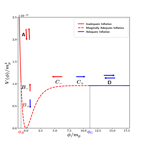
Figure 23: This figure schematically shows initial field values which lead to adequate and inadequate Starobinsky inflation. The initial energy scale is $H_{i}=3\times 10^{-3}m_{p}$. The solid blue line represents the region of adequate inflation while the solid red line displays the region of inadequate inflation. (Note that $\phi$ is unbounded on the right.) For initial field values lying in the interval $\phi_{i}\in[\phi_{B},\phi_{C}]$ (red dashed line), one gets adequate inflation only if the initial velocity $\dot{\phi_{i}}$ is positive. This figure shows that it is easy for inflation to commence from the flat right wing of the potential. Note that only a small portion of the full potential is shown in this figure.

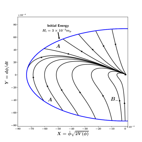
Figure 24: This figure illustrates the phase-space associated with the regions $A$ and $B_{-}$ on the steep left wing of the potential (62) illustrated in figure 23. As earlier, $Y=\dot{\phi}$ is plotted against $X=\hat{\phi}\sqrt{2V(\phi)}$ for the fixed initial energy scale $H_{i}=3\times 10^{-3}m_{p}$ (blue line). ($\hat{\phi}=\frac{\phi}{|\phi|}$ is the sign of field $\phi$.) Note that the horizontal slow-roll inflationary separatrix is absent which reflects the fact that commencing from region $A$ (and $B_{-}$) in figure 23, one cannot get adequate inflation from the steep left wing of the Starobinsky potential.

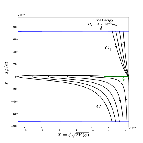
Figure 25: This figure illustrates the phase-space associated with the flat right wing of the potential (62). $Y=\dot{\phi}$ is plotted against $X=\hat{\phi}\sqrt{2V(\phi)}$ for the fixed initial energy scale $H_{i}=3\times 10^{-3}m_{p}$ (denoted by blue lines at the boundary). ($\hat{\phi}=\frac{\phi}{|\phi|}$ is the sign of field $\phi$.) Note that trajectories commencing at the boundary with $\dot{\phi_{i}}>0$ (region $C_{+}$ in figure 23) converge to the inflationary separatrix ‘S’ before winding up in spirals around the center (shown in detail in the next figure). By contrast, trajectories commencing on the right wing of $V(\phi)$ with $\dot{\phi_{i}}<0$ in the region $C_{-}$ in figure 23 , do not lead to inflation.

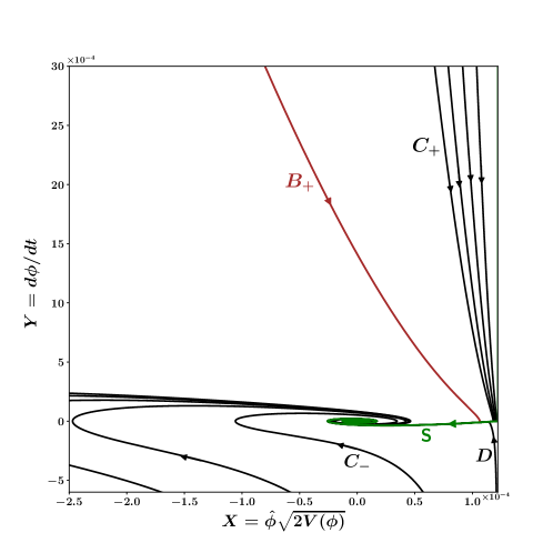
Figure 26: A zoomed-in view of the phase-space of Starobinsky inflation which highlights the existence of the slow-roll inflationary separatrix on the flat right wing (green line marked ‘S’ in figure 23). Most trajectories commencing on the right wing (from regions $C_{+}$ and $D$) converge to ‘S’ before spiralling in towards the minimum of $V(\phi)$. (The spirals correspond to post-inflationary oscillations.) Such an inflationary separatrix does not exist for the steep left wing of the potential. However note the brown trajectory which is able to meet the inflationary separatrix on the right wing even though it commences from region $B_{+}$ of $V(\phi)$ (but with $\dot{\phi_{i}}>0$) as shown in figure 23. The brown trajectory describes the motion of the field $\phi$ as it rolls up the potential.

The asymmetry of the potential (62) is reflected in the asymmetry of the phase-space shown in figures 24, 25, 26. The phase-space associated with region $A$ on the steep left wing of $V(\phi)$ shows no slow-roll and consequently does not possess an inflationary separatrix; see figure 24. The flat right wing of $V(\phi)$, on the other hand, has a slow-roll inflationary separatrix ‘S’ (shown by the green line in figures 25 and 26), towards which most trajectories converge; see figures 25, 26. Some of the lines commencing from the left wing with $\dot{\phi}>0$ initially, represented by $B_{+}$ in figure 23, (the brown line in figure 26) are also able to meet the inflationary separatrix giving rise to adequate inflation. These interesting features of Starobinsky inflation have been summarized in figure 23. In this figure, the solid blue line corresponding to $\phi_{i}\geq\phi_{C}$ shows trajectories which lead to adequate inflation regardless of the initial direction of $\dot{\phi_{i}}$. By contrast, the red region corresponding to $\phi_{i}\leq\phi_{B}$ reflects inadequate inflation. The intermediate region $\phi_{i}\in[\phi_{B},\phi_{C}]$ leads to adequate inflation only when the initial velocity is positive i.e.  $\dot{\phi_{i}}>0$ (dashed line). Dependence of $\phi_{B}$ and $\phi_{C}$ on the initial energy scale $H_{i}$ is shown in table 6.

$H_{i}$ (in $m_{p}$)	$\phi_{B}$ (in $m_{p}$)	$\phi_{C}$ (in $m_{p}$)
$3\times 10^{-3}$	$-0.28$	$11.11$
$3\times 10^{-2}$	$-2.16$	$12.99$
$3\times 10^{-1}$	$-4.04$	$14.87$

Table 6: Dependence of $\phi_{B}$ and $\phi_{C}$ on the initial energy scale $H_{i}$ for Starobinsky Inflation.

From table 6 one observes that $\phi_{B}$ shifts to lower (more negative) values as the initial energy scale of inflation, $H_{i}$, is increased. This is indicative of the fact that inflation can commence even from the steep left wing of $V(\phi)$ provided the scalar field has a sufficiently large positive velocity initially, which would enable the inflaton to climb up the flat right wing and result in inflation.

It may be noted that our results do not support some of the claims made in stein13 that inflation in plateau-like potentials suffers from an unlikeliness problem since only a small range of initial field values leads to adequate inflation. The authors of stein13 made this claim on the basis of a flat Mexican hat potential. Our analysis, based on more realistic models including Higgs inflation and Starobinsky inflation, has shown that, on the contrary, a fairly large range of initial field values (and initial energy scales) can give rise to adequate inflation, as illustrated in figures 16 and 23.

Finally we would like to draw attention to the fact that the phase-space analysis performed here for Starobinsky inflation is likely to carry over to the E-model $\alpha$-attractor potential E-model , since the two potentials are qualitatively very similar.

VI Discussion

In this paper we have addressed the issue of the robustness of inflation to different choices of initial conditions. We have widely varied the initial kinetic and potential terms $\frac{1}{2}{\dot{\phi}_{i}}^{2}$ and $V(\phi_{i})$ for a given initial energy scale of inflation and determined the fraction of initial conditions which give rise to adequate inflation ($N_{e}\geq 60$). Our analysis has primarily focussed on the following models: (i) chaotic inflation and its extensions such as monodromy inflation, (ii) Higgs inflation, (iii) Starobinsky inflation. For class (i) we have shown that inflation becomes more robust for lower values of the exponent $n$ in the inflaton potential $V\propto|\phi|^{n}$. This is illustrated in figure 11. Concerning (ii), it is well known that Higgs inflation can arise from a non-minimal coupling of the Higgs field to the Ricci scalar. In this case the effective inflaton potential in the Einstein frame is asymptotically flat and has plateau-like features for large absolute values of the inflaton field. This is also true in the Einstein frame representation of the Starobinsky potential, but in this case one of the wings of $V(\phi)$ is flat while the other is steep (and cannot sustain inflation). A remarkable feature which is shared by (non-minimally coupled) Higgs inflation and Starobinsky inflation, is that one can get adequate inflation ($N_{e}\geq 60$) even if the inflaton commences to roll from the minimum of the potential ($\phi=0$) and not from its periphery. This remarkable property is typical of asymptotically flat potentials and is not shared by the power law potentials commonly associated with chaotic inflation. This new insight forms one of the central results of our paper.

We also show that inflation can be sourced by a Higgs-like field provided the Higgs has a non-canonical kinetic term. In this case non-canonical inflation is more robust, and arises for a larger class of initial conditions, than canonical inflation.

Using phase space analysis we have shown that the fraction of trajectories which inflate increases with an increase in the value of the energy scale at which inflation commences. This observation appears to be generic and applies to all of the models which have been studied in this paper.

One might note that our analysis in this paper assumes a specific measure on the space of initial conditions. Namely we assume that $X=\hat{\phi}\sqrt{2V(\phi)}$ ($\hat{\phi}=\frac{\phi}{|\phi|}$ is the sign of field $\phi$) and $Y=\dot{\phi}$ are distributed uniformly at the boundary where initial conditions are set. Following this we determine the degree of inflation. While this approach follows the seminal work of belinsky85 , it is also possible to construct alternative measures. For instance one could assume instead that $\phi$ and $\dot{\phi}$ were distributed uniformly at the initial boundary. In this case the boundary will no more be a circle, as it was for chaotic inflation in figure 1. Instead its shape will crucially depend upon the form of $V(\phi)$. However we feel that as long as the initial phase-space distribution is not sharply peaked near specific values of $\phi_{i}$, $\dot{\phi}_{i}$, the broad results of our analysis will remain in place. (In other words we suspect that inflation is likely to remain generic for a large class of potentials, although we cannot prove this assertion.)

For the sake of simplicity we have confined our analysis of inflationary initial conditions to a spatially flat FRW universe. The reader should note that by restricting ourselves to homogeneous and isotropic cosmologies we do not address the larger problem of inflation in an inhomogeneous and anisotropic setting. Indeed, the issue as to whether inflation can successfully arise in a universe which is either inhomogeneous or anisotropic (or both) is rather complex and has been discussed in several papers including the recent review branden16 . In the case of a positive cosmological constant, it is well known that classical fluctuations in an FRW Universe redshift and disappear and the space-time approaches de Sitter space asymptotically gibbons . This result was extended to a ‘no-hair’ theorem by a consideration of more general space-times including the spatially homogeneous but anisotropic Bianchi I-VIII family which was shown to rapidly isotropize and (locally) approach de Sitter space in the future, provided all matter (with the exception of the cosmological constant) satisfied the strong energy condition wald_staro . The no-hair theorem was subsequently extended to inflationary cosmology in no-hair . However these studies primarily focussed on anisotropic models and did not include the effects of inhomogeneity for which even a semi-analytical treatment is difficult. A recent discussion of this issue within a numerical setting suggests that, for plateau-like potentials, inflationary expansion can arise even when the scale of inhomogeneity exceeds the hubble length provided the mean spatial curvature is not positive ekls15 (also see guth14 ). The exception to this rule is associated with scalar field variations which exceed the inflationary plateau region and regions with large positive spatial curvature. Overall it appears that the robustness of inflation (in relation to inhomogeneous initial data) is related to the fact that while strongly inhomogeneous overdense regions collapse to form black holes, underdense regions continue to expand enabling inflation to eventually commence. It therefore appears that for inhomogeneous models the inflationary slow-roll regime is a local but not global attractor branden16 .

Finally it is important to note that since the simplest models of inflation are not past-extendible borde_vilenkin , the origin of the inflationary scenario remains an important open question.

VII Acknowledgements

A.V.T is supported by RSF Grant 16-12-10401 and by the Russian Government Program of Competitive Growth of Kazan Federal University. A.V.T is thankful to IUCAA, where this research work has been carried out, for the hospitality. S.S.M. thanks the Council of Scientific and Industrial Research (CSIR), India, for financial support as senior research fellow. S.S.M would also like to thank Surya Narayan Sahoo, Remya Nair and Prasun Dutta for technical help in generating some of the figures. S.S.M would like to thank Sanil Unnikrishnan for useful discussions and comments on the non-canonical Higgs inflation section.

Appendix A The values of $n_{{}_{S}}$ and $r$ for several inflationary models

For single field slow-roll inflation, the amplitude of scalar fluctuations in given by baumann07

$$\Delta_{{}_{S}}^{2}=\frac{1}{24\pi^{2}}\frac{V(\phi_{*})}{m_{p}^{4}}\frac{1}{\epsilon(\phi_{*})}$$ (63)

where $\phi_{*}$ is the value of $\phi$ at $N_{e}$ e-foldings before the end of inflation. CMB observations CMB imply $\Delta_{{}_{S}}^{2}=2.2\times 10^{-9}$ so that

$$\frac{1}{24\pi^{2}}\frac{V(\phi_{*})}{m_{p}^{4}}\frac{1}{\epsilon(\phi_{*})}=2.2\times 10^{-9}~{}.$$ (64)

Similarly, for single field slow-roll inflation, the scalar spectral index is given by baumann07

$$n_{{}_{S}}=1+2\eta(\phi_{*})-6\epsilon(\phi_{*}),$$ (65)

and the tensor to scalar ratio is given by baumann07

$$r=16\epsilon(\phi_{*}).$$ (66)

Values of the CMB normalized parameters $n_{{}_{S}}$ and $r$ for some of the inflationary models discussed in this paper are listed in table 7, assuming $N_{e}=60$. The corresponding $r$ vs $n_{{}_{S}}$ plot is shown in figure 27.

Model	$V(\phi)$	Parameter	$n_{{}_{S}}$	$r$
Non-minimal Higgs	$V_{0}\left(1-e^{-\sqrt{\frac{2}{3}}\frac{|\phi|}{m_{p}}}\right)^{2}$	$V_{0}=9.6\times 10^{-11}~{}m_{p}^{4}$	$0.967$	$0.003$
Starobinsky	$\frac{3}{4}m^{2}m_{p}^{2}\left(1-e^{-\sqrt{\frac{2}{3}}\frac{\phi}{m_{p}}}\right)^{2}$	$m=1.13\times 10^{-5}~{}m_{p}$	$0.967$	$0.003$
Fractional Monodromy	$V_{0}\left|\frac{\phi}{m_{p}}\right|^{2/3}$	$V_{0}=3.34\times 10^{-10}~{}m_{p}^{4}$	$0.978$	$0.044$
Linear Monodromy	$V_{0}\left|\frac{\phi}{m_{p}}\right|$	$V_{0}=1.97\times 10^{-10}~{}m_{p}^{4}$	$0.975$	$0.066$
Quadratic Chaotic	$\frac{1}{2}m^{2}\phi^{2}$	$m=5.97\times 10^{-6}~{}m_{p}$	$0.967$	$0.132$
Quartic Chaotic	$\frac{\lambda_{c}}{4}\phi^{4}$	$\lambda_{c}=1.43\times 10^{-13}$	$0.951$	$0.262$

Table 7: This table lists the CMB normalized value of parameter, scalar spectral index $n_{{}_{S}}$ and tensor to scalar ratio $r$ for different single field slow-roll inflationary models considered in this paper.

For Higgs inflation, substitution of the value $V_{0}=9.6\times 10^{-11}~{}m_{p}$ into equation (44), gives $\xi=1.62\times 10^{4}$ for the non-minimal coupling parameter, which is in agreement with equation (33).

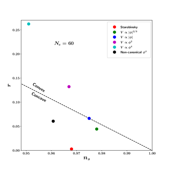
Figure 27: The values of tensor to scalar ratio $r$ and the corresponding values of scalar spectral index $n_{{}_{S}}$ are plotted in this figure for different inflationary potentials considered in this paper corresponding to $N_{e}=60$. Note that the values of $r$ and $n_{{}_{S}}$ for the Starobinsky inflation (62) and the Higgs inflation in the non-minimal framework (43) are same since both the potentials have the same functional form as far as the flat inflationary wing is concerned. The value for the non-canonical $\lambda\phi^{4}$ potential has been determined assuming $\alpha=5$ in (46).

Appendix B Jordan to Einstein frame transformation for Higgs inflation

A derivation of equations (38) and (39) is given below. Our derivation is similar to that given in kaiser , however we calculate the field transformation $\phi\longrightarrow\chi$ explicitly. We commence with the Jordan frame action (29), namely

$$S_{J}=\int d^{4}x\sqrt{-g}\bigg{[}f(\phi)R-\frac{1}{2}g^{\mu\nu}\partial_{\mu}\phi\partial_{\nu}\phi-U(\phi)\bigg{]}$$ (67)

which is described by the metric $g_{{\mu}{\nu}}$. The Einstein frame is described by $\hat{g}_{{\mu}{\nu}}$ where

$$\hat{g}_{{\mu}{\nu}}=\Omega^{2}g_{{\mu}{\nu}}$$ (68)

the conformal factor being given by

$$\Omega^{2}=\frac{2}{m_{p}^{2}}f(\phi)=1+\frac{\xi\phi^{2}}{m_{p}^{2}}~{}.$$ (69)

Furthermore $\sqrt{-g}$ transforms as

$$\sqrt{-g}\longrightarrow\sqrt{-\hat{g}}=\Omega^{4}\sqrt{-g}$$ (70)

and the Ricci scalar transforms as

$$R\longrightarrow\hat{R}=\frac{1}{\Omega^{2}}\Big{[}R-\frac{1}{\Omega}\Box\Omega\Big{]}$$ (71)

where

$$\Box\Omega=\frac{1}{\sqrt{-g}}\partial_{\mu}(\sqrt{-g}g^{{\mu}{\nu}}\partial_{\nu}\Omega).$$

As a result the action (67) transforms to

$$S=\int d^{4}x\sqrt{-\hat{g}}\bigg{[}\frac{m_{p}^{2}}{2}\hat{R}-\frac{1}{2}\hat{g}^{\mu\nu}(\frac{1}{\Omega^{2}}\partial_{\mu}\phi\partial_{\nu}\phi+\frac{6m_{p}^{2}}{\Omega^{2}}\partial_{\mu}\Omega\partial_{\nu}\Omega)-\frac{U(\phi)}{\Omega^{4}}\bigg{]}.$$ (72)

Notice that the coupling of the scalar field to gravity has become minimal. However the kinetic term is non-canonical. In order to change this to the canonical form one redefines the field $\phi\longrightarrow\chi$ such that

$$\frac{1}{2}\hat{g}^{\mu\nu}(\frac{1}{\Omega^{2}}\partial_{\mu}\phi\partial_{\nu}\phi+\frac{6m_{p}^{2}}{\Omega^{2}}\partial_{\mu}\Omega\partial_{\nu}\Omega)+\frac{U(\phi)}{\Omega^{4}}=\frac{1}{2}\hat{g}^{\mu\nu}\partial_{\mu}\chi\partial_{\nu}\chi+V(\chi)$$ (73)

where

$$V(\chi)=\frac{U[\phi(\chi)]}{\Omega^{4}}.$$ (74)

Consequently the action in the Einstein frame becomes

$$S_{E}=\int d^{4}x\sqrt{-\hat{g}}\bigg{[}\frac{m_{p}^{2}}{2}\hat{R}-\frac{1}{2}\hat{g}^{\mu\nu}\partial_{\mu}\chi\partial_{\nu}\chi-V(\chi)\bigg{]}.$$

Note that assuming a homogeneous and isotropic space-time one can drop the spatial derivative terms in (73) to get

$$\frac{1}{\Omega^{2}}\Big{[}\dot{\phi^{2}}+6m_{p}^{2}\dot{\Omega}^{2}\Big{]}=\dot{\chi}^{2}$$

$$\Rightarrow\frac{1}{\Omega^{2}}\Big{[}\dot{\phi^{2}}+6m_{p}^{2}(\frac{\partial\Omega}{\partial\phi})^{2}\dot{\phi}^{2}\Big{]}=(\frac{\partial\chi}{\partial\phi})^{2}\dot{\phi}^{2}$$

$$\Rightarrow(\frac{\partial\chi}{\partial\phi})^{2}=\frac{1}{\Omega^{4}}\Big{[}\Omega^{2}+\frac{6\xi^{2}\phi^{2}}{m_{p}^{2}}\Big{]}$$

$$\Rightarrow\frac{\partial\chi}{\partial\phi}=\pm\frac{1}{\Omega^{2}}\sqrt{\Omega^{2}+\frac{6\xi^{2}\phi^{2}}{m_{p}^{2}}}$$

which corresponds to (39). Note that the ’$\pm$’ sign here leads to the symmetric potential in figure 16.

Appendix C Derivation of asymptotic forms of the Higgs potential in the Einstein frame

Equations (39) and (74) can be rewritten as

$$\frac{\partial\chi}{\partial\phi}=\pm\frac{\sqrt{1+\frac{\xi\phi^{2}}{m_{p}^{2}}+\frac{6\xi^{2}\phi^{2}}{m_{p}^{2}}}}{1+\frac{\xi\phi^{2}}{m_{p}^{2}}}$$ (75)

$$V(\phi)=\frac{U[\phi(\chi)]}{\Omega^{4}}\simeq\frac{\frac{\lambda}{4}\phi^{4}}{\left(1+\frac{\xi\phi^{2}}{m_{p}^{2}}\right)^{2}}~{}.$$ (76)

Using these two equations we proceed to derive the following useful asymptotic formulae.

1. For $\phi\ll\sqrt{\frac{2}{3}}\frac{m_{p}}{\xi}$ one finds $\frac{\partial\chi}{\partial\phi}\simeq\pm 1$, consequently (76) simplifies to

   $$V(\chi)\simeq\frac{\lambda}{4}\chi^{4}.$$ (77)

2. For $\phi\gg\sqrt{\frac{2}{3}}\frac{m_{p}}{\xi}$ one finds $\frac{\partial\chi}{\partial\phi}\simeq\pm\frac{\sqrt{6}\frac{\xi\phi}{m_{p}}}{\Omega^{2}}$ where $\Omega^{2}=1+\frac{\xi\phi^{2}}{m_{p}^{2}}$. Hence in this case

   $$\chi\simeq\pm\sqrt{\frac{3}{2}}m_{p}\log{\Omega^{2}(\phi)}.$$ (78)

   For $\sqrt{\frac{2}{3\xi^{2}}}\ll\frac{\phi}{m_{p}}\ll\frac{1}{\sqrt{\xi}}$, expression (78) reduces to

   $$\chi\simeq\pm\sqrt{\frac{3}{2}}\frac{\xi\phi^{2}}{m_{p}},$$ (79)

   consequently the potential in (76) acquires the form

   $$V(\chi)\simeq\left(\frac{\lambda m_{p}^{2}}{6\xi^{2}}\right)\chi^{2}~{}.$$ (80)

   Finally for $\frac{\sqrt{\xi}\phi}{m_{p}}\gg 1$ one finds, from (78)

   $$\phi\simeq\frac{m_{p}}{\sqrt{\xi}}\exp\left(\frac{\pm\chi}{\sqrt{6}m_{p}}\right)$$ (81)

   where the ’$+$’ sign is taken for $\chi>0$ and the ’$-$’ sign is taken for $\chi<0$, since the above solution is valid only in the limit when $|\frac{\sqrt{\xi}\phi}{m_{p}}|\gg 1$. Consequently we can rewrite our solution as

   $$\phi\simeq\frac{m_{p}}{\sqrt{\xi}}\exp\left(\frac{|\chi|}{\sqrt{6}m_{p}}\right)~{},$$ (82)

   and the potential in (76) is given by

   $$V(\chi)\simeq\frac{\lambda m_{p}^{4}}{4\xi^{2}}\left(1+\exp\Big{[}-\sqrt{\frac{2}{3}}\frac{|\chi|}{m_{p}}\Big{]}\right)^{-2}.$$ (83)

   To summarize, the relation between $\chi$ and $\phi$ in the three asymptotic regions is given by

   $$\frac{\chi}{m_{p}}=\left\{\begin{array}[]{ll}\pm\frac{\phi}{m_{p}},\quad\frac{\phi}{m_{p}}\ll\sqrt{\frac{2}{3\xi^{2}}},\\ \pm\sqrt{\frac{3}{2}}\xi\left(\frac{\phi}{m_{p}}\right)^{2},\quad\sqrt{\frac{2}{3\xi^{2}}}\ll\frac{\phi}{m_{p}}\ll\frac{1}{\sqrt{\xi}},\\ \pm\sqrt{6}\log{\left(\frac{\sqrt{\xi}\phi}{m_{p}}\right)},\quad\frac{\phi}{m_{p}}\gg\frac{1}{\sqrt{\xi}}\end{array}\right.$$

References

- (1) A. A. Starobinsky, Phys. Lett. B 91, 99-102 (1980).
- (2) A. H. Guth, Phys. Rev. D 23, 347 (1981).
- (3) A. D. Linde, Phys. Lett. B 108, 389 (1982).
- (4) A. Albrecht and P.J. Steinhardt, Phys. Rev. Lett. 48, 1220 (1982).
- (5) A.D Linde, Particle Physics and Inflationary Cosmology, Harwood Academic (1990) [arXiv:hep-th/0503203]; A. R. Liddle and D.H. Lyth, Cosmological Inflation and Large Scale Structure, Cambridge University Press (2000); D. Baumann, TASI Lectures on Inflation, [arXiv:0907.5424].
- (6) V. F. Mukhanov and G. V. Chibisov, JETP Lett. 33, 532 (1981).
- (7) S. W. Hawking, Phys. Lett. B 115, 295 (1982).
- (8) A. A. Starobinsky, Phys. Lett. B 117, 175 (1982).
- (9) A. H. Guth and S. -Y. Pi, Phys. Rev. Lett. 49, 1110 (1982).
- (10) V. A. Belinsky, L. P. Grishchuk, I. M. Khalatnikov and Ya. B. Zeldovich, Phys. Lett. 155 B, 232 (1985).
- (11) V. A. Belinsky, H. Ishihara, I. M. Khalatnikov and H. Sato, Prog. Theor. Phys. 79, 676 (1988).
- (12) A. Ijjas, P. J. Steinhardt and A. Loeb, Phys. Lett. B 723, 261-266 (2013) [arXiv:1314.2785].
- (13) A. D. Linde, [arXiv:1710.04278].
- (14) S. Unnikrishnan, V. Sahni and A. Toporensky, JCAP 1208 (2012) 018 [arXiv:1205.0786].
- (15) R. Brandenberger, [arXiv:1601.01918].
- (16) P. A. R. Ade et al. (Planck Collaboration), Planck 2015 results. XX., Constraints on Inflation, Astron. Astrophys. 594, A20 [arXiv:1502.02114].
- (17) G N. Felder, A. V. Frolov, L. Koffman and A.D Linde, Phys. Rev. D 66, 023507 (2002) [arXiv:hep-th/0202017].
- (18) A. D. Linde, Phys. Lett. B 129, 177 (1983).
- (19) A .D. Linde, Prog. Theor. Phys. Suppl. 163, 295-322 (2006) [arXiv:hep-th/0503195].
- (20) E. Silverstein and A. Westphal, Phys. Rev. D 78, 106003 (2008) [arXiv:0803.3085].
- (21) L. McAllister, E. Silverstein and A. Westphal,Phys. Rev. D 82, 046003 (2010) [arXiv:0808.0706].
- (22) R. Flauger, L. McAllister, E. Pajer, A. Westphal and G. Xu, JCAP 1006, 009 (2010) [arXiv:0907.2916 [hep-th]].
- (23) M. A. Amin, R. Easther, H. Finkel, R. Flauger and M. P. Hertzberg, Phys. Rev. Lett. 108, 241302 (2012) [arXiv:1106.3335 [astro-ph.CO]].
- (24) K. Harigaya, M. Ibe, K. Schmitz and T. T. Yanagida, Phys. Lett. B 720, 125-129 (2013) [arXiv:1211.6241].
- (25) K. Harigaya, M. Ibe, K. Schmitz and T. T. Yanagida, Phys. Lett. B 733, 283-287 (2014), [arXiv:1403.4536].
- (26) K. Harigaya, M. Ibe, K. Schmitz and T. T. Yanagida, Phys. Rev. D 90, 123524 (2014) [arXiv:1407.3084].
- (27) C. Germani and A. Kehagias, Phys. Rev. Lett. 105, 011302 (2010); C. Germani and A. Kehagias, JCAP 05(2010)019; C. Germani and A. Kehagias, Phys. Rev. Lett. 106, 161302 (2011); C. Germani and Y. Yatanabe, JCAP 07(2011) 031; S. Tsujikawa, Phys. Rev. D 85, 083518 (2012).
- (28) F. L. Bezrukov and M. Shaposhnikov, Phys. Lett. B 659, 703-706 (2008) [arXiv:0710.3755].
- (29) R. Fakir and W.G. Williams, Phys. Rev. D 41, 1783-1791 (1990).
- (30) F. L. Bezrukov, D. Gorbunov and M. Shaposhnikov, JCAP 0906 (2009) 029 [arXiv:0812.3622].
- (31) J. García-Bellido, D. G. Figueroa, and J. Rubio, Phys. Rev. D 79, 063531 (2009) [arXiv:0812.4624].
- (32) D. P. George, S. Mooij and M. Postma, JCAP, 1402 (2014) 024 [arXiv:1310.2157].
- (33) Y. Ema, R. Jinno, K. Mukaida and K. Nakayama, JCAP 1702 (2017) no.2, 045 [arXiv:1609.05209].
- (34) D. I. Kaiser, Phys. Rev. D 81, 084044 (2010) [arXiv:1003.1159].
- (35) A. Salvio and A. Mazumdar, Phys. Lett. B 750, 194-200 (2015) [arXiv:1506.07520].
- (36) A. Salvio [arXiv:1712.04477].
- (37) R. Kallosh and A. Linde, JCAP07 (2013) 002 [arXiv:1306.5220].
- (38) V. Mukhanov and A. Vikman, JCAP 0602, 004 (2006) [arXiv:astro-ph/0512066].
- (39) B. Whitt, Phys. Lett. B 145, 176 (1984).
- (40) K. I. Maeda, Phys. Rev. D 37, 858 (1988).
- (41) D. S. Gorbunov and A. G. Panin, Phys. Lett. B 743, 79-81 (2015) [arXiv:1412.3407].
- (42) B. Bonga and B. Gupt, Phys. Rev. D 93, no.6, 063513 (2016) [arXiv:1510.04896].
- (43) R. Kallosh, A. Linde and D. Roest, JHEP11, 198 (2013) [arXiv:1311.0472].
- (44) G.W. Gibbons and S.W. Hawking, Phys. Rev. D 15 (1977) 2738; S.W. Hawking and I.G. Moss, Phys. Lett. B 110 (1982) 35; W. Boucher and G.W. Gibbons, in: The very early universe, eds.G.W. Gibbons, S.W. Hawking and S.T.C. Siklos, (Cambridge U.P., Cambridge, 1983).
- (45) R.M. Wald, Phys. Rev. D 28, 2118 (1983); A.A. Starobinsky, JETP Lett. 37, 66 (1983).
- (46) I. Moss and V. Sahni, Phys. Lett. B 178, 159 (1986); V. Sahni and L.A. Kofman, Phys. Lett. A 117, 275 (1986); Phys.Lett. A117, 275 (1986); J.D. Barrow, Phys. Lett. B 180, 335 (1986); J.D. Barrow, Phys. Lett. B 187, 12 (1987); M. Mijic and J.A. Stein-Schabes, Phys. Lett. B 203, 353 (1988); M. Mijic, M.S. Morris and Wai-Mo Suen, Phys. Rev. D 39, 1496 (1989); K. Olive, Phys.Rept. 190, 307 (1990); R.H. Brandenberger and J.H. Kung, Phys. Rev. D 42, 1008 (1990); D.S. Goldwirth, Phys. Rev. D 43, 3204 (1991); D.S. Goldwirth and T. Piran, Phys.Rept. 214, 223 (1992); Y. Kitada and Kei-ichi Maeda, Phys. Rev. D 45, 1416 (1992); Y. Kitada and Kei-ichi Maeda, Class.Quant.Grav. 10, 703 (1993); E. Calzetta and M. Sakellariadou, Phys. Rev. D 45, 2802 (1992); R. Maartens, V. Sahni and T. D. Saini, Phys. Rev. D 63, 063509 (2001) [arXiv:gr-qc/0011105]; C. Pitrou, T. S. Pereira and J.-P. Uzan, JCAP 0804 (2008) 004 [arXiv:0801.3596]; I. Ya. Aref’eva, N. V. Bulatov, L. V. Joukovskaya and S. Yu. Vernov, Phys. Rev. D 80, 083532 (2009) [arXiv:0903.5264]; H.-C. Kim and M. Minamitsuji, Phys. Rev. D 81, 083517 (2010), Erratum: Phys.Rev. D82 (2010) 109904 [arXiv:1002.1361]; H.-C. Kim and M. Minamitsuji, JCAP 1103 (2011) 038 [arXiv:1101.0329]; S. Hervik, D. F. Mota and M. Thorsrud, JHEP 1111 (2011) 146 [arXiv:1109.3456]; A. Maleknejad, M.M. Sheikh-Jabbari and J. Soda, JCAP 1201 (2012) 016 [arXiv:1109.5573]; J. Soda, Class.Quant.Grav. 29 (2012) 083001 [arXiv:1201.6434]; A. Maleknejad and M.M. Sheikh-Jabbari, Phys. Rev. D D85, 123508 (2012) [arXiv:1203.0219]; [arXiv:1203.0219]; A. Maleknejad and M.M. Sheikh-Jabbari, Phys.Rept. 528, 161 (2013) [arXiv:1212.2921].
- (47) W.E. East, M. Kleban, A. Linde and L. Senatore, JCAP 09(2016)010 [arXiv:1511.05143].
- (48) A.H. Guth, D.I. Kaiser, Y. Nomura, Phys. Lett. B 733, 112 (2014) [arXiv:1312.7619].
- (49) K. Dimopoulos and M. Artymowski, Astroparticle Physics, 94, 11 (2017) [arXiv:1610.06192]; M. Bastero-Gil, A. Berera, R. Brandenberger, I. G. Moss, R. O. Ramos, J. G. Rosa, JCAP 1801, 002 (2018) [arXiv:1612.04726].
- (50) J.J.M. Carrasco, R. Kallosh and A. Linde, Phys. Rev. D 92, 063519 (2015) [arXiv:1506.00936]; M. Artymowski, Z. Lalak and M. Lewicki, [arXiv:1607.01803].
- (51) A. Borde and A. Vilenkin, Phys. Rev. Lett. 72, 3305 (1994) [gr-qc/9312022]