Macdonald topological vertices and brane condensates

Abstract.

We show, in a number of simple examples, that Macdonald-type $qt$-deformations of topological string partition functions are equivalent to topological string partition functions that are without $qt$-deformations but with brane condensates, and that these brane condensates lead to geometric transitions.

1. Introduction

We recall the topological vertex, its refinements and deformations, and ask what the physical interpretation of a specific Macdonald-type deformation is.

1.1. A hierarchy of topological vertices

1.1.1. Abbreviations

To simplify the presentation, we use 1. string, string partition function, vertex, etc. for topological string, topological string partition function, topological vertex, etc., which should cause no confusion, as we only consider the latter, and use topological only for emphasis when that is needed, 2. $qt$-string partition function, $qt$-quantum curve, etc. for $qt$-deformed string partition function, $qt$-deformed quantum curve, etc. 3. refined as in refined partition functions, etc., when discussing objects that are refined in the sense of [9, 10, 35]; otherwise, no refinement should be inferred, and unrefined is used only for emphasis when that is needed, 4. the $qt$-version of $\cdots$ for the version of an object that is deformed in the sense of [58, 18], and 5. a brane condensate, or simply a condensate is a set of infinitely-many brane insertions.

1.1.2. The original vertex as a normalized 1-parameter generating function of plane partitions with fixed asymptotic boundaries

In [31], Iqbal introduced a systematic way to compute $A$-model string partition functions in terms of gluing copies of a trivalent topological vertex, and constructed a special case of that vertex where one of the three legs is trivial. In [2], Aganagic, Klemm, Mariño and Vafa constructed the full topological vertex $\mathcal{C}_{\,Y_{\,1}\,Y_{\,2}\,Y_{\,3}}\left\lgroup x\right\rgroup$, where all legs are non-trivial, that we refer to in the present work as the original vertex. It depends on a single parameter $x$, and a set of three Young diagrams, $Y_{\,1}$, $Y_{\,2}$ and $Y_{\,3}$, and has a combinatorial interpretation as a normalized partition function of 3D plane partitions [49], where each box in each plane partition is assigned a weight $x$. All plane partitions generated by $\mathcal{C}_{\,Y_{\,1}\,Y_{\,2}\,Y_{\,3}}\left\lgroup x\right\rgroup$ satisfy fixed asymptotic boundary conditions specified by $Y_{\,1}$, $Y_{\,2}$ and $Y_{\,3}$. Copies of $\mathcal{C}_{\,Y_{\,1}\,Y_{\,2}\,Y_{\,3}}\left\lgroup x\right\rgroup$ can be glued to form string partition functions. Using geometric engineering [38, 39], these string partition functions are identified with instanton partition functions in 5D supersymmetric gauge theories on $\mathbbm{R}^{4}\times S^{1}$, in a self-dual $\Omega$-background with Nekrasov parameters $\epsilon_{1}\,+\,\epsilon_{2}\,=\,0$ [44, 45]. Using the AGT/W correspondence [5, 59], the 4D limit of these 5D instanton partition functions are identified with conformal blocks in 2D conformal field theories with an integral central charge $c$.

1.1.3. The refined vertex as a normalized 2-parameter generating function of plane partitions with fixed asymptotic boundaries

In [9, 10], Awata and Kanno introduced a refined version of $\mathcal{C}_{\,Y_{\,1}\,Y_{\,2}\,Y_{\,3}}\left\lgroup x\right\rgroup$, and in [35], Iqbal, Kozcaz and Vafa introduced yet another refined version of the same object. In [7], Awata, Feigin and Shiraishi proved that these two refinements are equivalent. In the present work, we focus on the refined vertex $\mathcal{R}_{\,Y_{\,1}\,Y_{\,2}\,Y_{\,3}}\left\lgroup x,y\right\rgroup$ of [35]. It depends on two parameters $\left\lgroup x,y\right\rgroup$, and a set of three Young diagrams, $Y_{\,1}$, $Y_{\,2}$ and $Y_{\,3}$, and has a combinatorial interpretation as a normalized partition function of 3D plane partitions. Each box in each plane partition is assigned a weight $x$ or $y$ as follows. One splits each plane partition diagonally into vertical Young diagrams. Scanning the vertical Young diagrams from one end to the other, a box in a plane partition is assigned a weight $x$ if it belongs to a vertical Young diagram that protrude with respect to the preceding Young diagram, and a weight $y$ if it belongs to a vertical Young diagram that does not. All plane partitions generated by $\mathcal{R}_{\,Y_{\,1}\,Y_{\,2}\,Y_{\,3}}\left\lgroup x,y\right\rgroup$ satisfy fixed asymptotic boundary conditions specified by $Y_{\,1}$, $Y_{\,2}$ and $Y_{\,3}$. Copies of $\mathcal{R}_{\,Y_{\,1}\,Y_{\,2}\,Y_{\,3}}\left\lgroup x,y\right\rgroup$ can be glued to form refined string partition functions. Using geometric engineering [38, 39], these refined string partition functions are identified with instanton partition functions in 5D supersymmetric gauge theories on $\mathbbm{R}^{4}\times S^{1}$, in a generic $\Omega$-background, with Nekrasov parameters $\epsilon_{1}\,+\,\epsilon_{2}\,\neq\,0$ [44, 45]. Using the AGT/W correspondence [5, 59], the 4D limits of these 5D instanton partition functions are identified with conformal blocks in 2D conformal field theories with a non-integral central charge $c$.

1.1.4. The Macdonald vertex as a $qt$-deformation of the refined vertex

In [58], Vuletić introduced a deformation of MacMahon’s generating function of plane partitions, in terms of two Macdonald-type parameters $\left\lgroup q,t\right\rgroup$. This deformation is independent of the refinement introduced in [9, 10] and [35], as one can check by considering $\mathcal{R}^{\,\prime}_{\,\varnothing\,\varnothing\,\varnothing}\left\lgroup x,y\right\rgroup$, the unnormalized version of $\mathcal{R}_{\,\varnothing\,\varnothing\,\varnothing}\left\lgroup x,y\right\rgroup$, which is a refinement of MacMahon’s generating function, but is different from that of [58]. In [18], $\mathcal{R}_{\,Y_{\,1}\,Y_{\,2}\,Y_{\,3}}\left\lgroup x,y\right\rgroup$ was deformed using the same Macdonald-type parameters $\left\lgroup q,t\right\rgroup$ that were used in [58], to obtain the Macdonald vertex $\mathcal{M}_{\,Y_{\,1}\,Y_{\,2}\,Y_{\,3}}^{\,q\,t}\left\lgroup x,y\right\rgroup$. Copies of $\mathcal{M}_{\,Y_{\,1}\,Y_{\,2}\,Y_{\,3}}^{\,q\,t}\left\lgroup x,y\right\rgroup$ can be glued to form $qt$-string partition functions that are 5D $qt$-instanton partition functions. The latter have well-defined 4D-limits and, for generic values of $\left\lgroup q,t\right\rgroup$, contain infinite towers of poles for every pole that is present in the limit $q\rightarrow t$ [18].

1.1.5. Limits of the Macdonald vertex

In constructing the original and the refined vertex, (undeformed) free bosons that satisfy the Heisenberg algebra,

(1.1) $$\left[a_{m},a_{n}\right]=n\,\delta_{m+n,\,0}\,,$$

play a central role [49, 35]. Similarly, in constructing the Macdonald vertex, $qt$-free bosons that satisfy the $qt$-Heisenberg algebra,

(1.2) $$\left[a_{m}^{\,q\,t},a_{n}^{\,q\,t}\right]=n\,\left\lgroup\frac{1-q^{\,|n|}}{1-t^{\,|n|}}\right\rgroup\delta_{m+n,\,0}\,,$$

play a central role. In the limit $q\rightarrow t$, $\mathcal{M}_{\,Y_{\,1}\,Y_{\,2}\,Y_{\,3}}^{\,q\,t}\left\lgroup x,y\right\rgroup\rightarrow\,\mathcal{R}_{\,Y_{\,1}\,Y_{\,2}\,Y_{\,3}}\left\lgroup x,y\right\rgroup$, and in the limit $x\rightarrow y$, $\mathcal{M}_{\,Y_{\,1}\,Y_{\,2}\,Y_{\,3}}^{\,q\,t}\left\lgroup x,y\right\rgroup\rightarrow\,\mathcal{C}_{\,Y_{\,1}\,Y_{\,2}\,Y_{\,3}}^{\,q\,t}\left\lgroup x\right\rgroup$, which is a $qt$-deformation of $\mathcal{C}_{\,Y_{\,1}\,Y_{\,2}\,Y_{\,3}}\left\lgroup x\right\rgroup$.

1.2. The physical interpretation of the $qt$-deformation

It is clear by inspection of explicit computations that the Macdonald parameter ratio $q/t$ is a different object from either the $M$-theory circle radius $R$ or the refinement parameter ratio $x/y$. The purpose of the present work is to shed light on the geometric and/or physical interpretation of the $qt$-deformation. To do this, we consider simple string partition functions, and show that in $M$-theory terms, the deformation $q/t\neq 1$ describes a condensation of $M5$-branes that lead to geometric transitions that change the topology of the original Calabi-Yau 3-fold [23]. In conformal field theory terms, we expect that it describes a condensation of vertex operators that push the conformal field theory off criticality [60].

1.3. Outline of contents

In section 2, we include comments on notation used in the text, and definitions of combinatorial objects, including MacMahon’s generating function of plane partitions, its refinement and $qt$-deformation, and in 3, include basic facts related to the original topological vertex, the refined topological vertex, and their $qt$-deformations. In section 4, we give our first example of the equivalence of $qt$-deformation and brane condensation, which shows that the refined $qt$-string partition function on $\mathbbm{C}^{\,3}$ is equivalent to a refined string partition function on $\mathbbm{C}^{\,3}$ with no $qt$-deformation but in the presence of condensates, and in 5, we give our second example, which shows that a refined $qt$-deformed partition function on $\mathbbm{C}^{\,3}$ with a single-brane insertion is equivalent to its counterpart (also with a single-brane insertion) with no $qt$-deformation but in the presence of condensates. In section 6, we discuss the relation of the condensates and geometric transitions in the context of unrefined objects, and in 7, we discuss the $qt$-quantum curves associated with $qt$-partition function. Finally, in section 8, we collect a number of remarks, and discuss the various parameters that can appear in topological vertices and the relation with conformal field theory, and in appendix A, we collect useful skew Schur function identities that are used freely in the text.

2. Notation and definitions

We collect comments on notation, definitions of combinatorial objects, including variations on MacMahon’s generating function of plane partitions that appear in the sequel.

2.1. Notation

2.1.1. Deviations from standard notation

We use the variables $\left\lgroup x,y\right\rgroup$ as box weights/refinement parameters, instead of the variables $\left\lgroup q,t\right\rgroup$ used in [9, 10, 35]. We use $\mathcal{R}_{\,Y_{\,1}\,Y_{\,2}\,Y_{\,3}}\left\lgroup x,y\right\rgroup$ for the refined vertex instead of $\mathcal{C}_{\,Y_{\,1}\,Y_{\,2}\,Y_{\,3}}\left\lgroup t,q\right\rgroup$ as used in [35]. We reserve the variables $\left\lgroup q,t\right\rgroup$ for the Macdonald-type deformation parameters that appear in the Macdonald vertex $\mathcal{M}_{\,Y_{\,1}\,Y_{\,2}\,Y_{\,3}}^{\,q\,t}\left\lgroup x,y\right\rgroup$ of [18].

2.1.2. Sets

$\rho$ is the set of negative half-integers $\left\lgroup\rho_{\,1},\rho_{\,2},\ldots\right\rgroup$ with $\rho_{i}=-i+1/2$, that is $\left\lgroup\rho_{\,1},\rho_{\,2},\ldots\right\rgroup=\left\lgroup-\,1/2,-\,3/2,\ldots\right\rgroup$, and $\boldsymbol{\iota}$ is the set of non-zero positive integers $\left\lgroup 1,2,\ldots\right\rgroup$.

2.2. Combinatorics

2.2.1. Cells in the lower-right quadrant

Consider the lower-right quadrant in $\mathbbm{R}^{\,2}$, bounded by the right-half of the $x$-axis and the lower-half of the $y$-axis. The intersection point of the $x$- and $y$-axes to be the origin with coordinates $\left\lgroup 0,0\right\rgroup$, the $x$-coordinate increases to the right, the $y$-coordinate increases downwards. We divide this quadrant into cells of unit-length in each direction. A cell $\square$ has coordinates $\left\lgroup i,j\right\rgroup$, if the coordinates of the lower-right corner of the cell are $\left\lgroup i,j\right\rgroup$.

2.2.2. Young diagrams

$Y$ is a Young diagram in the lower-right quadrant of $\mathbbm{R}^{\,2}$ that consists of rows of cells of positive integral lengths $y_{\,1}\geqslant y_{\,2}\geqslant\cdots\geqslant 0$, and $Y^{\,\prime}$ is the transpose of $Y$ that consists of rows of cells of positive integral lengths $y_{\,1}^{\,\prime}\geqslant y_{\,2}^{\,\prime}\geqslant\cdots\geqslant 0$. $y_{\,1}^{\,\prime}$ is the number of (non-zero) parts in $Y$. The infinite profile of $Y$ consists of the union of 1. a semi-infinite line that extends from right to left along the positive, right-half of the $x$-axis, from $x=\infty$ to $x=y_{\,1}$, 2. the finite profile of $Y$, and 3. a semi-infinite line that extends from top to bottom along the positive, lower-half of the $y$-axis, from $y=y_{\,1}^{\,\prime}$ to $y=\infty$.

2.2.3. Arms, legs and hook lengths

Consider a Young diagram $Y$, and a cell $\square_{ij}$ with coordinates $\left\lgroup i,j\right\rgroup$ such that $\square_{ij}$ is not necessarily inside $Y$. The arm $A_{\,\square_{ij}}$, leg $L_{\,\square_{ij}}$, extended arm $A^{+}_{\,\square_{ij}}$, extended leg $L^{+}_{\,\square_{ij}}$, and hook $H_{\,\square_{ij}}$ of $\square_{ij}$, with respect to the infinitely-extended profile of $Y$, are,

(2.1) $$A_{\,\square_{ij}}=y_{i}-\,j,\quad L_{\,\square_{ij}}=y^{\,\prime}_{j}-\,i,\quad A^{+}_{\,\square_{ij}}=A_{\,\square_{ij}}+1,\quad L^{+}_{\,\square_{ij}}=L_{\,\square_{ij}}+1,\quad H_{\,\square_{ij}}=A_{\,\square_{ij}}+L_{\,\square_{ij}}+1,$$

where $y^{\,\prime}_{j}$ is the length of the $j$-row in $Y^{\,\prime}$, which is the $j$-column in $Y$. We also define,

(2.2) $$\left|Y\right|=\sum_{\square\in Y}\,1,\quad\frac{1}{2}\left\|Y\right\|^{\,2}=\sum_{\square\in Y}\left\lgroup A_{\,\square}+\frac{1}{2}\right\rgroup,\quad\frac{1}{2}\,\kappa_{\,Y}=\frac{1}{2}\left\lgroup\left\|Y\right\|^{\,2}-\left\|Y^{\,\prime}\right\|^{\,2}\right\rgroup=\sum_{\left\lgroup i,j\right\rgroup\in Y}\left\lgroup j-i\right\rgroup$$

2.3. The framing factor

We use the notation $f_{\,Y}\left\lgroup x\right\rgroup$ for the framing factor of the original vertex [43, 2],

(2.3) $$f_{\,Y}\left\lgroup x\right\rgroup=\left\lgroup-1\right\rgroup^{\left|Y\right|}\,x^{\frac{1}{2}\,\kappa_{\,Y}},$$

and,

(2.4) $$f_{\,Y}\left\lgroup x,y\right\rgroup=\left\lgroup-1\right\rgroup^{\left|Y\right|}\,x^{\,-\,\frac{1}{2}\,\left\|Y^{\,\prime}\right\|^{\,2}}\,y^{\,\frac{1}{2}\,\left\|Y\right\|^{\,2}},$$

for the refined framing factor introduced in [56] of the refined vertex.

2.4. Splitting indices

Starting from a sequence $\textbf{a}=\left\lgroup a_{1},a_{2},\ldots\right\rgroup$, one can split the single index $I$ of any element $a_{I}$ into two indices $ij$, so that $a_{I}\to a_{ij}$. One way to split the indices is in the following example.

2.4.1. Example

We proceed in two steps. 1. Position the elements of the 1-dimensional sequence $\left\lgroup a_{1},a_{2},\ldots\right\rgroup$ along the anti-diagonals of a 2-dimensional array, as in,

(2.5) $$\left\lgroup a_{1},a_{2},\ldots\right\rgroup\quad\mapsto\quad\begin{array}[]{cccc}a_{1}&a_{2}&a_{4}&\cdots\\ a_{3}&a_{5}&&\\ a_{6}&&&\\ \end{array}$$

2. Map the array with single-index elements to an array with double-index elements, where the double-indices are in conventional order, as in,

(2.6) $$\begin{array}[]{cccc}a_{1}&a_{2}&a_{4}&\cdots\\ a_{3}&a_{5}&&\\ a_{6}&&&\\ \end{array}\quad\mapsto\quad\begin{array}[]{cccc}a_{11}&a_{12}&a_{13}&\cdots\\ a_{21}&a_{22}&&\\ a_{31}&&&\\ \end{array}$$

Any such splitting of indices is far from unique. However, if the splitting rule is well-defined, as in (2.5)–(2.6), then it is bijective, and all such splittings are in bijection via the original 1-dimensional sequence.

2.5. Variations on MacMahon’s generating functions

2.5.1. Notation

To streamline the notation, we use the redundant notation $M_{\,x\,x}$ for MacMahon’s original generating function of plane partitions, so that we can write $M_{\,x\,y}$ for its refined counterpart, and $M_{\,x\,y}^{\,q\,t}$ for the $qt$-version of the latter. $M_{\,x\,x}^{\,q\,t}$ is the $qt$-MacMahon generating function of Vuletić, and $M_{\,x\,y}^{\,q\,q}=M_{\,x\,y}$.

2.5.2. $M_{\,x\,x}$

MacMahon’s generating function of plane partitions is,

(2.7) $$M_{\,x\,x}=\prod_{m\,=\,1}^{\infty}\left\lgroup\frac{1}{1-x^{\,m}}\right\rgroup^{\,m}=\exp{\left\lgroup\sum_{n\,=\,1}^{\infty}\frac{1}{n\left\lgroup x^{\,n/2}-x^{\,-\,n/2}\right\rgroup^{\,2}}\right\rgroup}$$

The first equation in (2.7) is the definition of the MacMahon generating function. The second is obtained by direct expansion of the logarithms of both sides. All refined and $qt$-versions of this equation, in the sequel, are proven similarly.

2.5.3. $M_{\,x\,y}$

The refined MacMahon’s generating function of plane partitions is [35],

(2.8) $$M_{\,x\,y}=\prod_{m,n=1}^{\infty}\frac{1}{1-x^{\,m}y^{\,n-1}}=\exp{\left\lgroup\sum_{n\,=\,1}^{\infty}\frac{\left\lgroup x/y\right\rgroup^{\,n/2}}{n\left\lgroup x^{\,n/2}-x^{\,-\,n/2}\right\rgroup\left\lgroup y^{\,n/2}-y^{\,-\,n/2}\right\rgroup}\right\rgroup}$$

In the limit $y\rightarrow x$, $M_{\,x\,y}\rightarrow M_{\,x\,x}$.

2.5.4. $M_{\,x\,x}^{\,q\,t}$

The $qt$-version MacMahon’s generating function of plane partitions is,

(2.9) $$M_{\,x\,x}^{\,q\,t}=\prod_{i\,=\,0}^{\infty}\prod_{m\,=\,1}^{\infty}\left\lgroup\frac{1-q^{\,i}tx^{\,m}}{1-q^{\,i}x^{\,m}}\right\rgroup^{\,m}=\exp{\left\lgroup\sum_{n\,=\,1}^{\infty}\frac{1}{n\left\lgroup x^{\,n/2}-x^{\,-\,n/2}\right\rgroup^{\,2}}\left\lgroup\frac{1-t^{n}}{1-q^{n}}\right\rgroup\right\rgroup}$$

which is the $qt$-MacMahon generating function introduced by Vuletić in [58]. In the limit $t\rightarrow q$, $M_{\,x\,x}^{\,q\,t}\rightarrow M_{\,x\,x}^{\,q\,q}=M_{\,x\,x}$.

2.5.5. $M_{\,x\,y}^{\,q\,t}$

The refined $qt$-version MacMahon’s generating function of plane partitions is [18],

(2.10) $$M_{\,x\,y}^{\,q\,t}=\prod_{i\,=\,0}^{\infty}\prod_{m,n=1}^{\infty}\frac{1-q^{\,i}\,t\,x^{\,m}\,y^{\,n-1}}{1-q^{\,i}x^{\,m}y^{\,n-1}}=\exp{\left\lgroup\sum_{n\,=\,1}^{\infty}\frac{\left\lgroup x/y\right\rgroup^{\,n/2}}{n\left\lgroup x^{\,n/2}-x^{\,-\,n/2}\right\rgroup\left\lgroup y^{\,n/2}-y^{\,-\,n/2}\right\rgroup}\left\lgroup\frac{1-t^{n}}{1-q^{n}}\right\rgroup\right\rgroup}$$

In the limit $y\rightarrow x$, $M_{\,x\,y}^{\,q\,t}=M_{\,x\,x}^{\,q\,t}$, and so on.

3. Topological vertices

We recall basic facts related to the topological vertices introduced in section 1.1.

3.1. The original vertex of [2]

With reference to the figure on the left in Fig. 3.1, the normalized version of the original vertex of [2] is,

(3.1) $$\mathcal{C}_{\,Y_{\,1}\,Y_{\,2}\,Y_{\,3}}\left\lgroup x\right\rgroup=x^{\,\frac{1}{2}\,\kappa_{Y_{\,1}}}\,s_{\,Y_{\,3}}\left\lgroup\,x^{\,\rho}\right\rgroup\sum_{\,Y}s_{\,Y_{\,1}^{\,\prime}/Y}\left\lgroup x^{\,\rho\,+\,Y_{\,3}}\right\rgroup s_{\,Y_{\,2}/Y}\left\lgroup x^{\,\rho\,+\,Y_{\,3}^{\,\prime}}\right\rgroup\\ =\left\lgroup-1\right\rgroup^{\,\left|Y_{\,2}\right|\,+\,\left|Y_{\,3}\right|}\,f_{\,Y_{\,1}}\left\lgroup x\right\rgroup x^{\,\frac{1}{2}\,\left\|Y_{\,3}\right\|^{\,2}}\left\lgroup\prod_{\square\in Y_{\,3}}\frac{1}{1-x^{\,H_{\,\square}}}\right\rgroup\sum_{\,Y}s_{\,Y_{\,1}/Y}\left\lgroup x^{\,-\,\rho\,-\,Y_{\,3}}\right\rgroup s_{\,Y_{\,2}^{\,\prime}/Y}\left\lgroup x^{\,-\,\rho\,-\,Y_{\,3}^{\,\prime}}\right\rgroup$$

Here $x^{\,\rho\,+\,Y}=\left\lgroup x^{\,\rho_{\,1}\,+\,y_{\,1}},x^{\,\rho_{\,2}\,+\,y_{\,2}},\ldots\right\rgroup$, $x=\mathrm{e}^{\,-\,g_{s}}$, where $g_{s}$ is the string coupling constant, and $s_{\,Y_{\,1}/Y_{\,2}}\left\lgroup\mathbf{x}\right\rgroup$ is the skew Schur function defined in terms of a pair of Young diagrams $\left\lgroup Y_{\,1},Y_{\,2}\right\rgroup$ and a set of possibly infinitely-many variables $\mathbf{x}=\left\lgroup x_{1},x_{2},\ldots\right\rgroup$. In the second equality, we have used the notation $f_{\,Y}\left\lgroup x\right\rgroup$ for the framing factor (2.3), and the identities in appendix A.

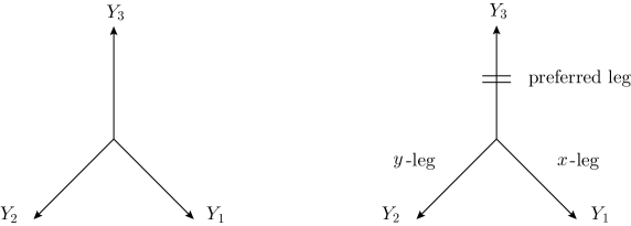
Figure 3.1. The figure on the left represents the vertex $\mathcal{C}_{\,Y_{\,1}\,Y_{\,2}\,Y_{\,3}}\left\lgroup x\right\rgroup$, and this vertex has the cyclic symmetry $\mathcal{C}_{\,Y_{\,1}\,Y_{\,2}\,Y_{\,3}}\left\lgroup x\right\rgroup=\mathcal{C}_{\,Y_{\,3}\,Y_{\,1}\,Y_{\,2}}\left\lgroup x\right\rgroup=\mathcal{C}_{\,Y_{\,2}\,Y_{\,3}\,Y_{\,1}}\left\lgroup x\right\rgroup$. The figure on the right represents the refined vertex $\mathcal{R}_{\,Y_{\,1}\,Y_{\,2}\,Y_{\,3}}\left\lgroup x,y\right\rgroup$ and the Macdonald vertex $\mathcal{M}_{\,Y_{\,1}\,Y_{\,2}\,Y_{\,3}}^{\,q\,t}\left\lgroup x,y\right\rgroup$. These two vertices break the cyclic symmetry and have the preferred leg. Note that $\mathcal{R}_{\,Y_{\,1}\,Y_{\,2}\,Y_{\,3}}\left\lgroup x,x\right\rgroup=\mathcal{C}_{\,Y_{\,1}\,Y_{\,2}\,Y_{\,3}^{\,\prime}}\left\lgroup x\right\rgroup$.

3.1.1. Normalization

$\mathcal{C}_{\,Y_{\,1}\,Y_{\,2}\,Y_{\,3}}\left\lgroup x\right\rgroup$ is normalized by $M_{\,x\,x}$ such that $\mathcal{C}_{\,\varnothing\,\varnothing\,\varnothing}\left\lgroup x\right\rgroup=1$. The unnormalized version is,

(3.2) $$\mathcal{C}^{\,\prime}_{\,Y_{\,1}\,Y_{\,2}\,Y_{\,3}}\left\lgroup x\right\rgroup=M_{\,x\,x}\,\mathcal{C}_{\,Y_{\,1}\,Y_{\,2}\,Y_{\,3}}\left\lgroup x\right\rgroup$$

3.1.2. $\mathcal{C}^{\,\prime}_{\,Y_{\,1}\,Y_{\,2}\,Y_{\,3}}\left\lgroup x\right\rgroup$ and $M_{\,x\,x}$ as partition functions

The unnormalized vertex $\mathcal{C}^{\,\prime}_{\,Y_{\,1}\,Y_{\,2}\,Y_{\,3}}\left\lgroup x\right\rgroup$ is the open topological $A$-model partition function on $\mathbbm{C}^{\,3}$ with three special Lagrangian submanifolds. $M_{\,x\,x}$ is the closed topological $A$-model partition function on $\mathbbm{C}^{\,3}$. The figure on the left in Fig. 3.1 is the toric web diagram of $\mathbbm{C}^{\,3}$.

3.1.3. Choice of framing

One can choose the framing of $\mathcal{C}_{\,Y_{\,1}\,Y_{\,2}\,Y_{\,3}}\left\lgroup x\right\rgroup$ as,

(3.3) $$\mathcal{C}_{\,Y_{\,1}\,Y_{\,2}\,Y_{\,3}}\left\lgroup x\right\rgroup\quad\to\quad\left\lgroup\prod_{\,i\,=\,1,\,2,\,3}f_{\,Y_{i}}\left\lgroup x\right\rgroup^{f_{i}}\right\rgroup\mathcal{C}_{\,Y_{\,1}\,Y_{\,2}\,Y_{\,3}}\left\lgroup x\right\rgroup,\quad f_{1},f_{2},f_{3}\in\mathbbm{Z},$$

where $f_{\,Y}\left\lgroup x\right\rgroup$ is the framing factor (2.3).

3.2. The refined vertex of [35]

With reference to the figure on the right in Fig. 3.1, the normalized refined vertex of [35] is,

(3.4) $$\mathcal{R}_{\,Y_{\,1}\,Y_{\,2}\,Y_{\,3}}\left\lgroup x,y\right\rgroup=\left\lgroup-1\right\rgroup^{\,\left|Y_{\,2}\right|\,+\,\left|Y_{\,3}\right|}\,f_{\,Y_{\,1}}\left\lgroup x,y\right\rgroup x^{\frac{1}{2}\left\|Y_{\,3}^{\,\prime}\right\|^{\,2}}\left\lgroup\prod_{\square\in Y_{\,3}}\frac{1}{1-x^{\,L^{+}_{\,\square}}y^{\,A_{\,\square}}}\right\rgroup\,\times\\ \sum_{Y}\left\lgroup\frac{y}{x}\right\rgroup^{\frac{1}{2}\left\lgroup|Y|-|Y_{\,1}|+|Y_{\,2}|\right\rgroup}s_{\,Y_{\,1}/Y}\left\lgroup y^{\,-\rho}x^{\,-Y_{\,3}^{\,\prime}}\right\rgroup s_{\,Y_{\,2}^{\,\prime}/Y}\left\lgroup x^{\,-\rho}y^{\,-Y_{\,3}}\right\rgroup,$$

where $f_{\,Y}\left\lgroup x,y\right\rgroup$ is the refined framing factor (2.4). In the limit $y\rightarrow x$,

(3.5) $$\mathcal{R}_{\,Y_{\,1}\,Y_{\,2}\,Y_{\,3}}\left\lgroup x,y\right\rgroup\quad\rightarrow\quad\mathcal{C}_{\,Y_{\,1}\,Y_{\,2}\,Y_{\,3}^{\,\prime}}\left\lgroup x\right\rgroup$$

3.2.1. Remark.

The dependence on the Young diagram $Y_{\,3}$ in $\mathcal{R}_{\,Y_{\,1}\,Y_{\,2}\,Y_{\,3}}\left\lgroup x,y\right\rgroup$ on the left hand side of (3.5) is replaced by a dependence on its transpose $Y_{\,3}^{\,\prime}$ in $\mathcal{C}_{\,Y_{\,1}\,Y_{\,2}\,Y_{\,3}^{\,\prime}}\left\lgroup x\right\rgroup$ on the right hand side.

3.2.2. Remark.

$\left\lgroup t,q\right\rgroup$ in [35] become $\left\lgroup x,y\right\rgroup$ in the present work, and the refined vertex $\mathcal{C}_{\,Y_{\,1}\,Y_{\,2}\,Y_{\,3}}\left\lgroup t,q\right\rgroup$ in [35] is related to $\mathcal{R}_{\,Y_{\,1}\,Y_{\,2}\,Y_{\,3}}\left\lgroup x,y\right\rgroup$ in the present work by,

(3.6) $$\mathcal{C}_{\,Y_{\,1}\,Y_{\,2}\,Y_{\,3}}\left\lgroup t,q\right\rgroup=\left\lgroup-1\right\rgroup^{|Y_{\,1}|+|Y_{\,2}|}\,f_{\,Y_{\,3}}\left\lgroup x,y\right\rgroup\mathcal{R}_{\,Y_{\,2}\,Y_{\,1}\,Y_{\,3}}\left\lgroup x,y\right\rgroup$$

3.2.3. Choice of framing

One can choose the framing of $\mathcal{R}_{\,Y_{\,1}\,Y_{\,2}\,Y_{\,3}}\left\lgroup x,y\right\rgroup$ as,

(3.7) $$\mathcal{R}_{\,Y_{\,1}\,Y_{\,2}\,Y_{\,3}}\left\lgroup x,y\right\rgroup\quad\to\quad\left\lgroup\prod_{i=1,2,3}f_{\,Y_{i}}\left\lgroup x,y\right\rgroup^{f_{i}}\right\rgroup\mathcal{R}_{\,Y_{\,1}\,Y_{\,2}\,Y_{\,3}}\left\lgroup x,y\right\rgroup,\quad f_{1},f_{2},f_{3}\in\mathbbm{Z}$$

3.2.4. Normalization

$\mathcal{R}_{\,Y_{\,1}\,Y_{\,2}\,Y_{\,3}}\left\lgroup x,y\right\rgroup$ is normalized by $M_{\,x\,y}$ such that $\mathcal{R}_{\,\varnothing\,\varnothing\,\varnothing}\left\lgroup x\right\rgroup=1$. The unnormalized version is,

(3.8) $$\mathcal{R}^{\,\prime}_{\,Y_{\,1}\,Y_{\,2}\,Y_{\,3}}\left\lgroup x,y\right\rgroup=M_{\,x\,y}\,\mathcal{R}_{\,Y_{\,1}\,Y_{\,2}\,Y_{\,3}}\left\lgroup x,y\right\rgroup$$

3.3. The Macdonald vertex of [18]

With reference to the figure on the right in Fig. 3.1, the normalized Macdonald vertex of [18] is,

(3.9) $$\mathcal{M}^{\,q\,t}_{\,Y_{\,1}\,Y_{\,2}\,Y_{\,3}}\left\lgroup x,y\right\rgroup=\left\lgroup\prod_{i\,=\,0}^{\infty}\prod_{\square\in Y_{\,3}}\frac{1-q^{\,i}\,t\,x^{\,L^{+}_{\,\square}}y^{\,A_{\square}}}{1-q^{\,i}\,x^{\,L^{+}_{\,\square}}y^{\,A_{\square}}}\right\rgroup\sum_{Y}P_{\,Y_{\,1}/Y}^{\,q\,t}\left\lgroup y^{\,\boldsymbol{\iota}-1}x^{\,-\,Y_{\,3}^{\,\prime}}\right\rgroup Q_{\,Y_{\,2}/Y}^{\,q\,t}\left\lgroup x^{\,\boldsymbol{\iota}}y^{\,-Y_{\,3}}\right\rgroup$$

Here $P_{\,Y_{\,1}/Y_{\,2}}^{\,q\,t}\left\lgroup\mathbf{x}\right\rgroup$ and $Q_{\,Y_{\,1}/Y_{\,2}}^{\,q\,t}\left\lgroup\mathbf{x}\right\rgroup$ are the skew Macdonald and dual Macdonald functions defined for a pair of Young diagrams $\left\lgroup Y_{\,1},Y_{\,2}\right\rgroup$ and a set of possibly infinitely-many variables $\mathbf{x}=\left\lgroup x_{1},x_{2},\ldots\right\rgroup$.

3.3.1. Choice of framing

No choice of framing of $\mathcal{M}^{\,q\,t}_{\,Y_{\,1}\,Y_{\,2}\,Y_{\,3}}\left\lgroup x,y\right\rgroup$ was discussed in [18], and none will be needed in the present work.

3.3.2. Normalization

$\mathcal{M}^{\,q\,t}_{\,Y_{\,1}\,Y_{\,2}\,Y_{\,3}}\left\lgroup x,y\right\rgroup$ is normalized by $M^{\,q\,t}_{\,x\,x}$ such that $\mathcal{M}^{\,q\,t}_{\,\varnothing\,\varnothing\,\varnothing}\left\lgroup x,y\right\rgroup=1$. The unnormalized version is,

(3.10) $$\mathcal{M}^{\,\prime\,q\,t}_{\,Y_{\,1}\,Y_{\,2}\,Y_{\,3}}\left\lgroup x,y\right\rgroup=M^{\,q\,t}_{\,x\,y}\,\mathcal{M}^{\,q\,t}_{\,Y_{\,1}\,Y_{\,2}\,Y_{\,3}}\left\lgroup x,y\right\rgroup$$

4. A $qt$-partition function from brane condensates

We give an example of a refined $qt$-deformed partition function that is obtained from its undeformed counterpart via brane condensation.

4.1. From $M5$-branes to surface operators

Consider $M$-theory on,

(4.1) $$\mathbbm{R}^{4}\times S^{1}\times X,$$

where $S^{1}$ is the $M$-theory circle, and $X$ is a local toric Calabi-Yau 3-fold such that the topological $A$-model on $X$ geometrically engineers a 5D $SU(N)$ supersymmetric gauge theory on $\mathbbm{R}^{4}\times S^{1}$ with $\left\lgroup\mathbbm{C}^{\,\times}\right\rgroup^{\,2}$-equivariant parameters $x,y$ acting on $\mathbbm{R}^{4}$ ($\Omega$-background) [38, 39]. We introduce $M5$-branes on the submanifold,

(4.2) $$\mathbbm{R}^{\,2}\times S^{1}\times L\subset\mathbbm{R}^{4}\times S^{1}\times X,$$

where $L\cong S^{1}\times\mathbbm{C}$ is a Lagrangian submanifold in $X$ [29] such that an end-point of $L$ is on an edge of the toric web diagram [3]. The $M5$-branes geometrically engineer simple-type half-BPS surface operators that reduce the gauge group to $SU(N-1)\times U(1)$ on the surface $\mathbbm{R}^{\,2}$ [27, 6, 13, 37].

4.2. From surface operators to primary-field vertex operators

The AGT/W correspondence [5, 59] relates a class of 4D $\mathcal{N}=2$ supersymmetric gauge theories on $\mathbbm{R}^{4}$ to 2D Toda conformal field theories. Each of these Toda conformal field theories is defined on a punctured Riemann surface that is related to the Seiberg-Witten curve of the gauge theory and to the mirror curve of the Calabi-Yau 3-fold $X$. The simple-type surface operators on the gauge theory side correspond to vertex operators that, in turn, correspond to the highest-weight states in irreducible fully-degenerate highest-weight representations on the conformal field theory side [4, 17]. In other words, the $M5$-branes in (4.2) correspond to primary-field vertex operators of fully-degenerate representations in Toda conformal field theory [40, 17, 57, 8]. From that it follows that a condensation of the $M5$-branes corresponds to a condensation of vertex operators. We expect that such a condensation leads to an off-critical deformation of the chiral blocks in the conformal field theory of the type that leads to correlation functions in off-critical integrable models. We will say more about this in section 8. In the following we show that for $X=\mathbbm{C}^{3}$, $M5$-brane condensates lead to the refined $qt$-MacMahon generating function (2.10).

4.3. A $qt$-partition function from two brane condensates

4.3.1. The normalized version of the computation

Starting from the refined open-string partition function on $\mathbbm{C}^{3}$, which is the refined vertex, we trivialize the Young diagram on one of the three legs, and add a stack of infinitely-many branes on each of the two other legs. The first stack has open-string moduli $\mathbf{a}=\left\lgroup a_{1},a_{2},\ldots\right\rgroup$, and framing factor $f_{1}$, and the second has $\mathbf{b}=\left\lgroup b_{1},b_{2},\ldots\right\rgroup$, and framing factor $f_{2}$, as indicated in Fig. 4.1. The result is the open-string partition function,

(4.3) $$Z_{\,x\,y}^{\,\left\lgroup f_{1},\,f_{2}\right\rgroup}\left\lgroup\mathbf{a},\mathbf{b}\right\rgroup=\mathcal{N}_{\,\textit{branes}}\,\sum_{Y_{\,1},Y_{\,2}}\left\lgroup\prod_{i=1,2}f_{\,Y_{i}}\left\lgroup x,y\right\rgroup^{f_{i}}\right\rgroup\mathcal{R}_{\,Y_{\,1}\,Y_{\,2}\,\varnothing}\left\lgroup x,y\right\rgroup s_{\,Y_{\,1}}\left\lgroup\mathbf{a}\right\rgroup s_{\,Y_{\,2}}\left\lgroup\mathbf{b}\right\rgroup,$$

where $\mathcal{N}_{\,\textit{branes}}$ is a normalization factor, due to the introduction of the branes to be determined in the sequel. Choosing $\left\lgroup f_{1},f_{2}\right\rgroup=\left\lgroup-1,0\right\rgroup$ we get

(4.4) $$Z_{\,x\,y}^{\,\left\lgroup-1,\,0\right\rgroup}\left\lgroup\mathbf{a},\mathbf{b}\right\rgroup=\mathcal{N}_{\,\textit{branes}}\,\sum_{Y_{\,1},Y_{\,2},Y}v^{\,-|Y|}\,s_{\,Y_{\,1}/Y}\left\lgroup y^{\,-\rho}\right\rgroup s_{\,Y_{\,1}}\left\lgroup v\mathbf{a}\right\rgroup s_{\,Y_{\,2}^{\,\prime}/Y}\left\lgroup x^{\,-\rho}\right\rgroup s_{\,Y_{\,2}}\left\lgroup-v^{-1}\mathbf{b}\right\rgroup,$$

where $v=\left\lgroup x/y\right\rgroup^{1/2}$. Using the Cauchy identities in appendix A we obtain,

(4.5) $$Z_{\,x\,y}^{\,\left\lgroup-1,\,0\right\rgroup}\left\lgroup\mathbf{a},\mathbf{b}\right\rgroup=\mathcal{N}_{\,\textit{branes}}\,\left\lgroup\prod_{I,J=1}^{\infty}\left\lgroup 1-v^{-1}a_{I}b_{J}\right\rgroup\right\rgroup\left\lgroup\prod_{I=1}^{\infty}\frac{L\left\lgroup v^{-1}\,b_{I},x\right\rgroup}{L\left\lgroup v\,a_{I},y\right\rgroup}\right\rgroup,$$

where $L\left\lgroup a,x\right\rgroup$ is the quantum dilogarithm,

(4.6) $$L\left\lgroup a,x\right\rgroup=\prod_{m\,=\,1}^{\infty}\left\lgroup 1-a\,x^{\,m-\frac{1}{2}}\right\rgroup=\exp{\left\lgroup\sum_{n\,=\,1}^{\infty}\frac{a^{n}}{n\left\lgroup x^{\,n/2}-x^{\,-\,n/2}\right\rgroup}\right\rgroup}$$

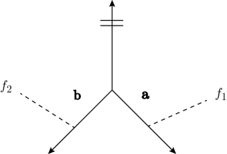
Figure 4.1. The vertex with two brane stacks with open-string moduli $\mathbf{a}=\left\lgroup a_{I}\right\rgroup_{I=1,2,\ldots}$, $\mathbf{b}=\left\lgroup b_{I}\right\rgroup_{I=1,2,\ldots}$ and framing factors $f_{1}$ and $f_{2}$.

The partition function (4.5) includes the contribution of the brane-brane interactions across the brane-stacks. To remove this contribution, we take the normalization factor $\mathcal{N}_{\,\textit{branes}}$ to be,

(4.7) $$\mathcal{N}_{\,\textit{branes}}=\prod_{I,J=1}^{\infty}\frac{1}{\left\lgroup 1-v^{-1}a_{I}b_{J}\right\rgroup},$$

and obtain the partition function without the brane-brane interactions,

(4.8) $$Z_{\,x\,y}^{\,\left\lgroup-1,\,0\right\rgroup}\left\lgroup\mathbf{a},\mathbf{b}\right\rgroup=\prod_{I=1}^{\infty}\frac{L\left\lgroup v^{-1}b_{I},x\right\rgroup}{L\left\lgroup va_{I},y\right\rgroup},\quad v=\left\lgroup\frac{x}{y}\right\rgroup^{1/2}$$

4.3.2. The unnormalized version of the computation

The above calculation started from the normalized vertex $\mathcal{R}_{\,Y_{1}\,Y_{2}\,Y_{3}}\left\lgroup x,y\right\rgroup$. If we use the unnormalized vertex $\mathcal{R}^{\,\prime}_{\,Y_{1}\,Y_{2}\,Y_{3}}\left\lgroup x,y\right\rgroup$ in (3.8), we get the unnormalized partition function with a single-brane insertion and two condensates,

(4.9) $$Z_{\,x\,y}^{\,\prime\,\left\lgroup-1,\,0\right\rgroup}\left\lgroup\mathbf{a},\mathbf{b}\right\rgroup=M_{\,x\,y}\prod_{I=1}^{\infty}\frac{L\left\lgroup v^{-1}b_{I},x\right\rgroup}{L\left\lgroup va_{I},y\right\rgroup}$$

Splitting the index $I\to(i,j)$, as in section 2.4, and setting,

(4.10) $$a_{I}\,\to\,a_{ij}=q^{\,i}\,x^{j-\frac{1}{2}},\quad b_{I}\,\to\,b_{ij}=q^{i-1}\,t\,x\,y^{j-\frac{3}{2}},\quad i,j=1,2,\ldots,$$

we find,

(4.11) $$Z_{\,x\,y}^{\,\prime\,\left\lgroup-1,\,0\right\rgroup}\left\lgroup a_{ij},b_{ij}\right\rgroup=M_{\,x\,y}\prod_{i,j=1}^{\infty}\frac{L\left\lgroup v^{-1}b_{ij},x\right\rgroup}{L\left\lgroup va_{ij},y\right\rgroup}=\prod_{i\,=\,0}^{\infty}\prod_{m,n=1}^{\infty}\frac{1-q^{\,i}tx^{\,m}y^{n-1}}{1-q^{\,i}x^{\,m}y^{n-1}}=M_{\,x\,y}^{\,q\,t}$$

We conclude that the refined open-string partition function on $\mathbbm{C}^{3}$ with two condensates, with moduli as in (4.10), agrees with the refined $qt$-MacMahon generating function $M_{\,x\,y}^{\,q\,t}$ in (2.10) which gives the refined $qt$-deformed closed string partition function on $\mathbbm{C}^{3}$. By taking the unrefined limit $y\to x$ in (4.11), we obtain,

(4.12) $$Z_{\,x\,x}^{\,\prime\,\left\lgroup-1,\,0\right\rgroup}\left\lgroup a_{ij},b_{ij}\right\rgroup=M_{\,x\,x}\prod_{i,j=1}^{\infty}\frac{L\left\lgroup b_{ij},x\right\rgroup}{L\left\lgroup a_{ij},x\right\rgroup}=\prod_{i\,=\,0}^{\infty}\prod_{m\,=\,1}^{\infty}\left\lgroup\frac{1-q^{\,i}tx^{\,m}}{1-q^{\,i}x^{\,m}}\right\rgroup^{\,m}=M_{\,x\,x}^{\,q\,t},$$

where the right hand side is the $qt$-MacMahon generating function (2.9) of Vuletić [58], and the left hand side can be derived using the original vertex $\mathcal{C}_{\,Y_{1}\,Y_{2}\,Y_{3}}\left\lgroup x\right\rgroup$ as in [28].

4.3.3. Remark

The relations (4.11) and (4.12) agree with the result that conformal blocks computed using $\mathcal{M}^{\,q\,t}_{\,Y_{1}\,Y_{2}\,Y_{3}}\left\lgroup x,y\right\rgroup$ are equal to those computed using $\mathcal{R}_{\,Y_{1}\,Y_{2}\,Y_{3}}\left\lgroup x,y\right\rgroup$ up to a $qt$-dependent factor [18].

5. A $qt$-partition function with a single-brane insertion from brane condensates

We give an example of a refined $qt$-deformed partition function with a single-brane insertion that is obtained from its undeformed counterpart via brane condensation.

5.1. A partition function with two brane condensates and a single-brane insertion

Consider the same partition function as in section 4.3, but now with an additional single brane (on the preferred leg of the refined vertex that has no brane-stacks) with an open-string modulus $U$ and a framing factor $f_{3}$, and two brane stacks, as represented in Fig. 5.1,

(5.1) $$Z^{\,\left\lgroup f_{1},\,f_{2},\,f_{3}\right\rgroup}_{\,x\,y}\left\lgroup U;\mathbf{a},\mathbf{b}\right\rgroup=\\ \mathcal{N}_{\,\textit{branes}}\,\sum_{Y_{\,1},Y_{\,2},Y_{\,3}}\left\lgroup\prod_{i=1,2,3}f_{\,Y_{i}}\left\lgroup x,y\right\rgroup^{f_{i}}\right\rgroup\mathcal{R}_{\,Y_{\,1}\,Y_{\,2}\,Y_{\,3}}\left\lgroup x,y\right\rgroup s_{\,Y_{\,1}}\left\lgroup\mathbf{a}\right\rgroup s_{\,Y_{\,2}}\left\lgroup\mathbf{b}\right\rgroup s_{\,Y_{\,3}^{\,\prime}}\left\lgroup U\right\rgroup$$

Here $\mathcal{N}_{\,\textit{branes}}$ is the normalization factor introduced in (4.3) and determined in (4.7), and the Schur function $s_{\,Y_{\,3}}\left\lgroup U\right\rgroup$ with a single variable $U$ is non-zero only for Young diagrams with a single row $y_{\,1}=d$. Choosing the framing factors as $\left\lgroup f_{1},f_{2},f_{3}\right\rgroup=\left\lgroup-1,0,f\right\rgroup$, we get,

(5.2) $$Z^{\,\left\lgroup-1,\,0,\,f\right\rgroup}_{\,x\,y}\left\lgroup U;\mathbf{a},\mathbf{b}\right\rgroup=\\ \mathcal{N}_{\,\textit{branes}}\,\sum_{Y_{\,1},Y_{\,2},Y_{\,3},Y}f_{\,Y_{\,3}^{\,\prime}}\left\lgroup x,y\right\rgroup^{f}x^{\,\frac{1}{2}\left\|Y_{\,3}\right\|^{\,2}}\left\lgroup\prod_{\square\in Y_{\,3}}\frac{1}{1-x^{\,A^{+}_{\,\square}}y^{\,L_{\,\square}}}\right\rgroup s_{\,Y_{\,3}}\left\lgroup-U\right\rgroup\,\times\\ v^{\,-|Y|}\,s_{\,Y_{\,1}/Y}\left\lgroup y^{\,-\rho}x^{\,-Y_{\,3}}\right\rgroup s_{\,Y_{\,1}}\left\lgroup v\mathbf{a}\right\rgroup s_{\,Y_{\,2}^{\,\prime}/Y}\left\lgroup x^{\,-\rho}y^{\,-Y_{\,3}^{\,\prime}}\right\rgroup s_{\,Y_{\,2}}\left\lgroup-v^{-1}\mathbf{b}\right\rgroup,$$

where $v=\left\lgroup x/y\right\rgroup^{1/2}$. Using the Cauchy identities in appendix A, we obtain,

(5.3) $$Z_{\,x\,y}^{\,\left\lgroup-1,\,0,\,f\right\rgroup}\left\lgroup U;\mathbf{a},\mathbf{b}\right\rgroup=\mathcal{N}_{\,\textit{branes}}\,\left\lgroup\prod_{I,J=1}^{\infty}\left\lgroup 1-v^{-1}a_{I}b_{J}\right\rgroup\right\rgroup\left\lgroup\prod_{I=1}^{\infty}\frac{L\left\lgroup v^{-1}b_{I},x\right\rgroup}{L\left\lgroup va_{I},y\right\rgroup}\right\rgroup\,\times\\ \sum_{d\,=\,0}^{\infty}\frac{x^{\frac{1}{2}\left\lgroup 1-f\right\rgroup\,d^{\,2}}\left\lgroup\left\lgroup-1\right\rgroup^{f+1}y^{\,f/2}\,U\right\rgroup^{\,d}}{\prod_{m\,=\,1}^{\,d}\left\lgroup 1-x^{\,m}\right\rgroup}\left\lgroup\prod_{I=1}^{\infty}\frac{\left\lgroup 1-a_{I}x^{\,\frac{1}{2}}\right\rgroup}{\left\lgroup 1-a_{I}x^{\,\frac{1}{2}-d}\right\rgroup}\prod_{m\,=\,1}^{\,d}\frac{\left\lgroup 1-b_{I}x^{\,m-1}y^{\,-\,\frac{1}{2}}\right\rgroup}{\left\lgroup 1-b_{I}x^{\,m-1}y^{\,\frac{1}{2}}\right\rgroup}\right\rgroup,$$

where $L\left\lgroup a,x\right\rgroup$ is the quantum dilogarithm in (4.6).

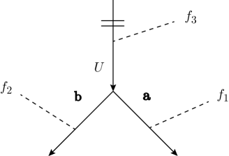
Figure 5.1. The partition function with a single-brane insertion that has an open-string modulus $U$ and framing factor $f_{3}$, and two brane stacks that have open-string moduli $\mathbf{a}=\left\lgroup a_{1},a_{2},\ldots\right\rgroup$, $\mathbf{b}=\left\lgroup b_{1},b_{2},\ldots\right\rgroup$ and framing factors $\left\lgroup f_{1},f_{2}\right\rgroup$. By the inverse arrow in the preferred leg we assign the transpose $Y_{\,3}^{\,\prime}$ of the Young diagram $Y_{\,3}$, where we note the relation $\mathcal{R}_{\,Y_{\,1}\,Y_{\,2}\,Y_{\,3}}\left\lgroup x,x\right\rgroup=\mathcal{C}_{\,Y_{\,1}\,Y_{\,2}\,Y_{\,3}^{\,\prime}}\left\lgroup x\right\rgroup$ in (3.5).

5.1.1. Normalization

Dividing the partition function with two condensates and a single-brane insertion by its counterpart that has no single-brane insertion (4.5), we obtain the normalized partition function,

(5.4) $$Z_{\,x\,y}^{\,\prime\,\left\lgroup-1,\,0,\,f\right\rgroup}\left\lgroup U;\mathbf{a},\mathbf{b}\right\rgroup=\\ \sum_{d\,=\,0}^{\infty}\frac{x^{\,\frac{1}{2}\,\left\lgroup 1-f\right\rgroup{d^{\,2}}}\left\lgroup\left\lgroup-1\right\rgroup^{\,f+1}\,y^{\,f/2}\,U\right\rgroup^{\,d}}{\prod_{m\,=\,1}^{\,d}\left\lgroup 1-x^{\,m}\right\rgroup}\left\lgroup\prod_{I=1}^{\infty}\frac{\left\lgroup 1-a_{I}\,x^{\frac{1}{2}}\right\rgroup}{\left\lgroup 1-a_{I}\,x^{\frac{1}{2}-d}\right\rgroup}\prod_{m\,=\,1}^{\,d}\frac{\left\lgroup 1-b_{I}\,x^{\,m-1}\,y^{-\frac{1}{2}}\right\rgroup}{\left\lgroup 1-b_{I}\,x^{\,m-1}\,y^{\,\frac{1}{2}}\right\rgroup}\right\rgroup$$

We now show that for a suitable choice of the moduli $\left\lgroup a_{1},a_{2},\ldots\right\rgroup$ and $\left\lgroup b_{1},b_{2},\ldots\right\rgroup$, the normalized partition function (5.4) of a single-brane insertion and two condensates is the $qt$-deformation of the partition function on $\mathbbm{C}^{\,3}$ with a single-brane insertion (and no condensates). The latter without the $qt$-deformation is obtained from (5.4) by setting the open-string moduli of the condensates to zero,

(5.5) $$Z_{\,x\,y}^{\,\prime\,\left\lgroup-1,\,0,\,f\right\rgroup}\left\lgroup U;0,0\right\rgroup=\\ \sum_{d\,=\,0}^{\infty}\frac{x^{\,\frac{1}{2}\,\left\lgroup 1-f\right\rgroup{d^{\,2}}}\left\lgroup\left\lgroup-1\right\rgroup^{f+1}\,y^{\,f/2}\,U\right\rgroup^{\,d}}{\prod_{m\,=\,1}^{\,d}\left\lgroup 1-x^{\,m}\right\rgroup}$$

5.1.2. Remark

Using the specialization of the one-row Schur function,

(5.6) $$s_{\,\left\lgroup d\right\rgroup}\left\lgroup x^{\,\rho}\right\rgroup=x^{\,\frac{1}{2}\,d\left\lgroup d-1\right\rgroup}\,s_{\,\left\lgroup 1^{\,d}\right\rgroup}\left\lgroup x^{\,\rho}\right\rgroup=\frac{\left\lgroup-1\right\rgroup^{\,d}x^{\,d^{\,2}/2}}{\prod_{m\,=\,1}^{\,d}\left\lgroup 1-x^{\,m}\right\rgroup},$$

the partition function (5.5) is expressed in terms of Schur functions as,

(5.7) $$\begin{split}Z_{\,x\,y}^{\,\prime\,\left\lgroup-1,\,0,\,f\right\rgroup}\left\lgroup U;0,0\right\rgroup&=\sum_{Y}x^{\,-\frac{1}{2}\,f\,d^{\,2}}s_{\,Y}\left\lgroup x^{\,\rho}\right\rgroup s_{\,Y}\left\lgroup\left\lgroup-1\right\rgroup^{f}\,y^{\,\frac{1}{2}\,f}\,U\right\rgroup\\ &=\sum_{Y}x^{\,\frac{1}{2}\left\lgroup 1-f\right\rgroup d^{\,2}}s_{\,Y^{\,\prime}}\left\lgroup x^{\,\rho}\right\rgroup s_{\,Y}\left\lgroup\left\lgroup-1\right\rgroup^{f}\,x^{\,-\frac{1}{2}}\,y^{\,\frac{1}{2}\,f}\,U\right\rgroup\end{split}$$

Using the Cauchy identities in appendix A, the special cases of (5.5) that correspond to $f=0,1$, satisfy,

(5.8) $$Z_{\,x\,y}^{\,\prime\,\left\lgroup-1,\,0,\,0\right\rgroup}\left\lgroup U;\,0,\,0\right\rgroup=\left\lgroup Z_{\,x\,y}^{\,\prime\,\left\lgroup-1,\,0,\,1\right\rgroup}\left\lgroup v\,U;\,0,\,0\right\rgroup\right\rgroup^{-1}=L\left\lgroup U,x\right\rgroup$$

5.2. The $qt$-deformation of $Z_{\,x\,y}^{\,\prime\,\left\lgroup-1,\,0,\,1\right\rgroup}\left\lgroup U;\,0,\,0\right\rgroup$

The $qt$-partition function on $\mathbbm{C}^{\,3}$ with a single-brane insertion with an open-string modulus $U$, can be computed using the Macdonald vertex as,

(5.9) $$Z_{\,x\,y}^{\,q\,t}\left\lgroup U\right\rgroup=\sum_{Y}\mathcal{M}_{\,\varnothing\,\varnothing\,Y}^{\,q\,t}\left\lgroup x,y\right\rgroup s_{\,Y^{\,\prime}}\left\lgroup U\right\rgroup=\sum_{d\,=\,0}^{\infty}\left\lgroup\prod_{i\,=\,0}^{\infty}\prod_{m\,=\,1}^{\,d}\frac{1-q^{\,i}\,t\,x^{\,m}}{1-q^{\,i}\,x^{\,m}}\right\rgroup U^{\,d}$$

Using $Z_{\,x\,y}^{\,\prime\,\left\lgroup-1,\,0,\,1\right\rgroup}\left\lgroup y^{\,-\frac{1}{2}}U;\,0,\,0\right\rgroup=Z_{\,x\,y}^{\,q\,q}\left\lgroup U\right\rgroup$, this $qt$-partition function can be considered as the $qt$-deformation of the undeformed partition function (5.5).

5.3. Identification

To identify the partition function in (5.4) with that in (5.9), we make the choice of moduli,

(5.10) $$a_{I}\,\to\,a^{\,\prime}_{ij}=x^{\,d}\,a_{ij}=q^{\,i}\,x^{j-\frac{1}{2}+d},\quad b_{I}\,\to\,b^{\,\prime}_{ij}=y\,b_{ij}=q^{\,i-1}\,t\,x\,y^{j-\frac{1}{2}},\quad i,j=1,2,\ldots$$

instead of that in (4.10). In other words, in this case, the moduli of the condensates now depend on the length of the single-row Young diagram that labels the Schur function that characterizes the single-brane insertion, $d$. For this modified choice of moduli, the normalized partition function (5.4) with a single-brane insertion and two condensates becomes,

(5.11) $$Z_{\,x\,y}^{\,\prime\,\left\lgroup-1,\,0,\,f\right\rgroup}\left\lgroup y^{\,-\,\frac{1}{2}\,f}U;\,a^{\,\prime}_{ij},\,b^{\,\prime}_{ij}\right\rgroup=\sum_{d\,=\,0}^{\,\infty}x^{\,\frac{1}{2}\,\left\lgroup 1-f\right\rgroup{d^{\,2}}}\left\lgroup\prod_{i\,=\,0}^{\infty}\prod_{m\,=\,1}^{\,d}\frac{1-q^{\,i}\,t\,x^{\,m}}{1-q^{\,i}\,x^{\,m}}\right\rgroup\left\lgroup\left\lgroup-1\right\rgroup^{f+1}U\right\rgroup^{\,d},$$

and we find,

(5.12) $$Z_{\,x\,y}^{\,\prime\,\left\lgroup-1,\,0,\,1\right\rgroup}\left\lgroup y^{\,-\,\frac{1}{2}}U;\,a^{\,\prime}_{ij},\,b^{\,\prime}_{ij}\right\rgroup=\sum_{d\,=\,0}^{\infty}\left\lgroup\prod_{i\,=\,0}^{\infty}\prod_{m\,=\,1}^{\,d}\frac{1-q^{\,i}\,t\,x^{\,m}}{1-q^{\,i}\,x^{\,m}}\right\rgroup U^{\,d}=Z_{\,x\,y}^{\,q\,t}\left\lgroup U\right\rgroup$$

We conclude that the refined $qt$-partition function with a single-brane insertion (and no condensates) coincides with its undeformed counterpart (with condensates) for a suitable choice of the framing factors, and of the open-string moduli of the condensates. Note that this refined $qt$-partition function does not depend on $y$, and coincides with the result computed by the original vertex $\mathcal{C}_{\,Y_{\,1}\,Y_{\,2}\,Y_{\,3}}\left\lgroup x\right\rgroup$ in a similar way.

5.3.1. Remark

We interpret the change in the choice of the moduli of the condensates from that in (4.10) to that in (5.10) as a back-reaction of the condensates to the single-brane insertion.

5.3.2. Remark

We have shown that the $qt$-deformed partition functions (2.10) and (5.9) are obtained, in the absence of a $qt$-deformation, from the partition functions (4.9) and (5.4), respectively. These results depend on the chosen specializations (4.10) and (5.10) that were made to obtain results that can be clearly interpreted. A study of the special significance (if any) of the choices that were made and the consequences of more general choices is beyond the scope of the present work.

6. $qt$-Deformations as geometric transitions

We discuss the relation of the brane condensates and geometric transitions in the context of unrefined objects.

6.1. Brane condensates and geometric transitions

Following Gomis and Okuda [21, 22], brane insertions change the topology of a Calabi-Yau 3-fold via a geometric transition [23], and a Calabi-Yau 3-fold with brane insertions is equivalent to a bubbling Calabi-Yau 3-fold of a more complicated topology, but without brane insertions. Correspondingly, an interpretation of the result in section 4.3 is that a condensate (which is a set of infinitely-many brane insertions) changes the topology of $\mathbbm{C}^{3}$ via a geometric transition, and $\mathbbm{C}^{3}$ with condensates is equivalent to another Calabi-Yau 3-fold of a more complicated geometry, but without condensates. To test this interpretation, we consider the $qt$-MacMahon generating function $M^{\,q\,t}_{\,x\,x}$ in (2.9), which, as we showed in section 4.3, is equal to the open-string partition on $\mathbbm{C}^{3}$ with two condensates, and interpret it as an undeformed (no condensates) closed string partition function on a Calabi-Yau 3-fold with more complicated topology than $\mathbbm{C}^{3}$.

6.2. Gopakumar-Vafa invariants

The partition function $Z_{X}\left\lgroup x,\,\mathbf{Q}\right\rgroup$ of the string on a Calabi-Yau 3-fold $X$ with (exponentiated) Kähler moduli $\mathbf{Q}$, is the generating function of Gopakumar-Vafa invariants $n_{\,\beta,\,g}\in\mathbbm{Z}$ [24],

(6.1) $$Z_{X}\left\lgroup x,\,\mathbf{Q}\right\rgroup=\exp\left\lgroup\sum_{\beta\,\in\,H_{2}\left\lgroup X,\,\mathbbm{Z}\right\rgroup}\,\sum_{g\,=\,0}^{\infty}\,\sum_{n\,=\,1}^{\infty}\,\frac{n_{\,\beta,\,g}}{n}\,\left\lgroup x^{\,n/2}-x^{\,-\,n/2}\right\rgroup^{2\,g\,-\,2}\mathbf{Q}^{\,\beta\,n}\right\rgroup,$$

where we have followed the notation used in [42]. Namely, if $i=\left\lgroup 1,2,\ldots,b_{2}\right\rgroup$, where $b_{2}$ is the second Betti number of $X$, $S_{i}$ is a basis of the second homology group $H_{2}\left\lgroup X,\,\mathbbm{Z}\right\rgroup$, and $Q_{i}$ are (exponentiated) Kähler parameters, then for any $\beta=\sum_{i}n_{i}[S_{i}]\in\,H_{2}\left\lgroup X,\,\mathbbm{Z}\right\rgroup$, $n_{i}\in\mathbbm{Z}$, $\mathbf{Q}^{\,\beta}=\prod_{i}Q_{\,i}^{\,n_{i}}$. Comparing $M^{\,q\,t}_{\,x\,x}$ in (2.9) normalized by $M_{\,x\,x}$ in (2.7) and the expansion in (6.1), we find that $n_{\,\beta,\,0}=\pm\,1$, $n_{\,\beta,\,g}=0$, for $g=1,2,\ldots$, which are the Gopakumar-Vafa invariants of a genus-0 manifold with infinitely-many homology 2-cycles $\beta$. From (4.10), the infinitely-many branes (in the unrefined case) have holonomies,

(6.2) $$\log a_{ij}=g_{s}\,\left\lgroup i\,N_{q}-j+\frac{1}{2}\right\rgroup,\quad\log b_{ij}=g_{s}\,\left\lgroup(i-1)\,N_{q}+N_{t}-j+\frac{1}{2}\right\rgroup,$$

where $g_{s}=-\log x$, $g_{s}N_{q}=\log q$, $g_{s}N_{t}=\log t$, and according to [21, 22], after large $N_{q}$ and $N_{t}$ limit, this yields a Calabi-Yau 3-fold via the bubbling. This agrees with our interpretation of the $qt$-deformation in terms of a geometric transition driven by a condensate, that is, the insertion of infinitely-many branes. In section 7, we identify this geometry with that of an infinite strip, but before we do that, we consider a simple, but important example.

6.3. A simple example of a geometric transition

In the special case of $q=0$, $t\neq 0$, the $qt$-MacMahon generating function (2.9) is,

(6.3) $$M^{\,0\,t}_{\,x\,x}=M_{\,x\,x}\,\prod_{m\,=\,1}^{\infty}\left\lgroup 1-t\,x^{\,m}\,\right\rgroup^{\,m}$$

This coincides with the undeformed closed string partition function on the resolved conifold, which is the total space of $\mathcal{O}(-1)\oplus\mathcal{O}(-1)\to\mathbb{P}^{1}$ with a single (exponentiated) Kähler modulus $t$, in agreement with the interpretation of the $t$-deformation of the MacMahon’s generating function proposed in [55]. From the perspective of this section, what we have is the simple geometric transition in Fig. 6.1.

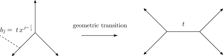
Figure 6.1. The figure on the left represents the partition function with a single-brane insertion on $\mathbbm{C}^{\,3}$. The figure on the right represents the closed string partition function on the resolved conifold. They are related by a geometric transition.

7. $qt$-Quantum curves

We discuss the $qt$-quantum curves associated with the unrefined limit of the refined $qt$-deformed partition function with a single-brane insertion in section 5.

7.1. The quantum curve for $Z^{\,q\,t}\left\lgroup U\right\rgroup$

7.1.1. Two operators

In the following, we need the operators $\widehat{U}$ and $\widehat{V}$, where $\widehat{U}$ acts as multiplication by a variable $U$, and $\widehat{V}$ acts as,

(7.1) $$\widehat{V}:=x^{\,U\frac{d}{dU}},$$

and satisfy the $x$-Weyl relation,

(7.2) $$\widehat{V}\,\widehat{U}\,=\,x\,\widehat{U}\,\widehat{V}$$

7.1.2. The quantum curve

The operators $\widehat{U}$ and $\widehat{V}$ act on $Z^{\,q\,t}\left\lgroup U\right\rgroup$, the unrefined limit of the refined $qt$-partition function with a single-brane insertion (5.9), as,

(7.3) $$\widehat{U}\,Z^{\,q\,t}\left\lgroup U\right\rgroup=U\,Z^{\,q\,t}\left\lgroup U\right\rgroup,\quad\widehat{V}\,Z^{\,q\,t}\left\lgroup U\right\rgroup=Z^{\,q\,t}\left\lgroup xU\right\rgroup$$

From (7.3), it follows that $Z^{\,q\,t}\left\lgroup U\right\rgroup$ satisfies the $x$-difference equation,

(7.4) $$\widehat{A}^{\,q\,t}\left\lgroup\widehat{U},\widehat{V}\right\rgroup\,Z^{\,q\,t}\left\lgroup U\right\rgroup:=\left\lgroup\prod_{i\,=\,0}^{\infty}\left\lgroup 1-q^{\,i}\widehat{V}\right\rgroup-\widehat{U}\prod_{i\,=\,0}^{\infty}\left\lgroup 1-q^{\,i}tx\widehat{V}\right\rgroup\right\rgroup\,Z^{\,q\,t}\left\lgroup U\right\rgroup=0,$$

which is the quantum curve related to $Z^{\,q\,t}\left\lgroup U\right\rgroup$. As discussed below, (7.4) is a $qt$-version of the quantum curve of $\mathbbm{C}^{\,3}$ in string theory [1, 16, 15, 26].

7.1.3. The classical limit of the quantum curve

Assuming that the asymptotic expansion of $Z^{\,q\,t}\left\lgroup U\right\rgroup$ in the classical limit, $g_{s}=-\log x\to 0$, has the WKB-form,

(7.5) $$Z^{\,q\,t}\left\lgroup U\right\rgroup\sim\exp{\left\lgroup-\,\frac{1}{g_{s}}\,\int^{\,U}\log V\left\lgroup U^{\,\prime}\right\rgroup\,\frac{dU^{\,\prime}}{U^{\,\prime}}\right\rgroup},$$

then $V\left\lgroup U\right\rgroup$ is a solution of the equation,

(7.6) $$A^{\,q\,t}\left\lgroup U,V\left\lgroup U\right\rgroup\right\rgroup:=\prod_{i\,=\,0}^{\infty}\left\lgroup 1-q^{\,i}V\left\lgroup U\right\rgroup\right\rgroup-U\prod_{i\,=\,0}^{\infty}\left\lgroup 1-q^{\,i}tV\left\lgroup U\right\rgroup\right\rgroup=0,$$

which is the classical curve related to $Z^{\,q\,t}\left\lgroup U\right\rgroup$. This curve can be identified with the mirror curve related to the infinite-strip geometry that consists of an infinite chain of $\left\lgroup-1,-1\right\rgroup$-curves, see the figure on the left in Fig. 7.1 [33] (see also [20]). This infinite-strip geometry agrees with the picture of condensates in sections 4, 5 and 6. In the remainder of this section, we consider a number of spacial cases of quantum curves.

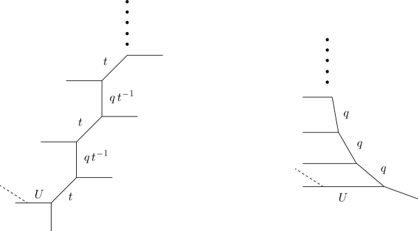
Figure 7.1. The figure on the left describes the infinite chain of $\left\lgroup-1,-1\right\rgroup$ curves with Kähler moduli $t$ and $qt^{-1}$, and a brane insertion with the open-string modulus $U$. The figure on the right describes the infinite chain of $\left\lgroup-2,0\right\rgroup$ curves with Kähler moduli $q$, and a brane insertion with the open-string modulus $U$.

7.2. Case 1

Choosing $q=t$, the partition function with a single-brane insertion (5.9) reduces to the undeformed partition function $Z_{\,x\,x}^{\,\prime\,\left\lgroup-1,\,0,\,1\right\rgroup}\left\lgroup x^{\,-\frac{1}{2}}U;\,0,\,0\right\rgroup$ with a single-brane insertion on $\mathbbm{C}^{\,3}$ in (5.5),

(7.7) $$Z^{\,q\,q}\left\lgroup U\right\rgroup=\sum_{d\,=\,0}^{\infty}\frac{1}{\prod_{m\,=\,1}^{\,d}\left\lgroup 1-x^{\,m}\right\rgroup}\,U^{\,d}=Z_{\,x\,x}^{\,\prime\,\left\lgroup-1,\,0,\,1\right\rgroup}\left\lgroup x^{\,-\frac{1}{2}}U;\,0,\,0\right\rgroup=L\left\lgroup x^{-\frac{1}{2}}U,x\right\rgroup^{-1},$$

and we find the quantum curve,

(7.8) $$\left\lgroup 1-\widehat{V}-\widehat{U}\right\rgroup\,Z^{\,q\,q}\left\lgroup U\right\rgroup=0$$

The classical limit, $g_{s}\to 0$, of the quantum curve (7.8) gives a mirror curve of $\mathbbm{C}^{\,3}$ [3],

(7.9) $$1-U-V=0$$

In other words, the $qt$-quantum curve (7.4) is a $qt$-version of the quantum curve (7.8), and (7.6) is a $qt$-version of the mirror curve (7.9).

7.3. Case 2

Choosing $q=0$ and $t\neq 0$, the partition function with a single-brane insertion (5.9) reduces to,

(7.10) $$Z^{\,0\,t}\left\lgroup U\right\rgroup=\sum_{d\,=\,0}^{\infty}\left\lgroup\prod_{m\,=\,1}^{\,d}\frac{1-t\,x^{\,m}}{1-x^{\,m}}\right\rgroup U^{\,d},$$

and we find the $t$-version of the quantum curve of $\mathbbm{C}^{\,3}$,

(7.11) $$\left\lgroup 1-\widehat{V}-\widehat{U}+t\,\widehat{V}\,\widehat{U}\right\rgroup\,Z^{\,0\,t}\left\lgroup U\right\rgroup=0$$

Note that $Z^{\,0\,t}\left\lgroup U\right\rgroup$ agrees with the undeformed partition function with a single-brane insertion, up to framing ambiguities, on the resolved conifold with the Kähler modulus $t$ [55], and the classical limit, $g_{s}\to 0$, of the quantum curve (7.11) is the mirror curve of the resolved conifold [3],

(7.12) $$1-U-V+t\,U\,V=0$$

In other words, the $t$-deformation of $\mathbbm{C}^{\,3}$ is the resolved conifold as discussed in section 6.3.

7.4. Case 3

Choosing $q\neq 0$ and $t=0$, the partition function with a single-brane insertion (5.9) reduces to,

(7.13) $$Z^{\,q\,0}\left\lgroup U\right\rgroup=\sum_{d\,=\,0}^{\infty}\frac{1}{\prod_{i\,=\,0}^{\infty}\prod_{m\,=\,1}^{\,d}\,\left\lgroup 1-\,q^{\,i}\,x^{\,m}\right\rgroup}\,U^{\,d},$$

and the $q$-version of the quantum curve of $\mathbbm{C}^{\,3}$ is,

(7.14) $$\left\lgroup\prod_{i\,=\,0}^{\infty}\left\lgroup 1-q^{\,i}\,\widehat{V}\right\rgroup-\widehat{U}\right\rgroup\,Z^{\,q\,0}\left\lgroup U\right\rgroup=0$$

$Z^{\,q\,0}\left\lgroup U\right\rgroup$ agrees with the undeformed partition function with a single-brane insertion, up to framing ambiguities and a slight modification of the Kähler moduli, for the infinite chain of $\left\lgroup-2,0\right\rgroup$-curves,

(7.15) $$\mathcal{O}\left\lgroup-2\right\rgroup\,\oplus\,\mathcal{O}\left\lgroup 0\right\rgroup\to\mathbb{P}^{1},$$

with the same Kähler modulus $q$ for all $\mathbb{P}^{1}$, see the figure on the right in Fig. 7.1 [33] (see also [20]). This infinite-strip geometry can be obtained from that in the figure on the left in Fig. 7.1 by suitable blow-downs. The classical limit, $g_{s}\to 0$, of the quantum curve (7.14) is the mirror curve of this strip geometry,

(7.16) $$\prod_{i\,=\,0}^{\infty}\left\lgroup 1-q^{\,i}\,V\right\rgroup\,-\,U=0$$

We conclude that the $q$-deformation of $\mathbbm{C}^{\,3}$ is identified with the infinite-strip geometry in the figure on the right in Fig. 7.1, and that this infinite-strip geometry is the result of a geometric transition caused by the condensates.

8. Remarks

We collect a number of remarks, with particular attention to the interpretation of the various parameters that can appear in topological vertices, and to the relation with conformal field theory.

8.1. The AGT counterpart of brane condensates

We showed that the Macdonald-type $qt$-deformation introduced in [58], when applied to topological string partition functions [18], leads to $qt$-partition functions that are equivalent to partition functions without a $qt$-deformation but with condensates. These condensates are surface operator condensates, and their counterparts on the conformal field theory side of the AGT correspondence are vertex operator condensates in 2D chiral conformal blocks. While this has not been studied in any detail, we expect that these vertex operator condensates play, at the level of conformal blocks, the same role that switching-on off-critical perturbations plays, at the level of the correlation functions [60], and that results in correlation functions in 2D off-critical integrable models. This expectation coincides with the results in [11, 12, 47, 48, 51].

8.2. Four parameters

If we start from a 4D instanton partition function in the absence of an $\Omega$-background, or an AGT-equivalent conformal block in a Gaussian 2D conformal field theory with an integral central charge, there are four known ways to modify such a partition function, or conformal block, and each of these ways is characterized by a parameter.

8.2.1. The radius of the $M$-theory circle, $R$

Topological string partition functions are 5D objects, and the corresponding instanton partition functions live in $\mathbbm{R}^{4}\times S^{1}$, where $S^{1}$ is the $M$-theory circle. For small $R$, one can think of the 5D instanton partition functions as $R$-deformations of their 4D limits, in the sense that switching on $R$ gradually is equivalent to including the lighter Kaluza-Klein modes that are infinitely-massive in the $R\rightarrow 0$, and that acquire finite masses as $R$ increases [32]. In 2D conformal field theory terms, switching $R$ on is equivalent to deforming the chiral conformal blocks away from criticality to obtain expectation values of type-I vertex operators [14], in some off-critical integrable statistical mechanical models [11, 12, 47, 48, 51].

8.2.2. The refinement parameter $x/y$

Starting with 4D instanton partition functions in the absence of an $\Omega$-background, one can switch on Nekrasov’s $\Omega$-deformation parameters, that is $\epsilon_{1}+\epsilon_{2}\neq 0$. In the presence of a finite $M$-theory circle of radius $R$, setting $x=e^{\,-\,R\,\epsilon_{1}}$, and $y=R^{\,R\,\epsilon_{2}}$, this refinement is equivalent to setting $x/y\neq 1$. In 2D conformal field theory terms, we modify the central charge of the conformal field theory while preserving conformal invariance, and the underlying statistical mechanical model remains critical.

8.2.3. The Macdonald deformation parameter $q/t$

The $q/t$-deformation of [58, 18] is yet another perturbation but, so far, no interpretation of this deformation is known. The purpose of this work is to offer one such interpretation.

8.2.4. The elliptic nome $p$

In [61, 19], two versions were proposed of a topological vertex based on Saito’s elliptic deformation of the quantum toroidal algebra $U_{q}\left\lgroup\widehat{\widehat{gl_{1}}}\right\rgroup$ [52, 53, 54]. In addition to the refinement parameters $\left\lgroup x,y\right\rgroup$, and the Macdonald-type deformation parameters $\left\lgroup q,t\right\rgroup$, this vertex depends on an elliptic nome parameter $p$ and copies of the $\left\lgroup q=t\right\rgroup$-limit of this vertex can be glued to obtain elliptic conformal blocks. The latter are equal to the elliptic conformal blocks that were computed in [36, 46] by gluing copies of the refined vertex of [35], then gluing pairs of external legs.

8.3. Three off-critical deformations

Aside from the refinement parameter $x/y$, which preserves criticality, it appears that we have three parameters that push the underlying 2D conformal blocks off-criticality, namely the $M$-theory circle radius $R$, the Macdonald parameter $q/t$, and the nome parameter $p$. One can show by explicit computation that these three parameters coexist and that their effects are different, but it remains unclear how to interpret these effects in statistical mechanics terms.

8.4. BPS states in $M$-theory

Following [24, 50], topological string partition functions on a Calabi-Yau 3-fold encode the degeneracies of the BPS states in $M$-theory compactified on the Calabi-Yau 3-fold, and the interpretation of the $xy$-refinement (of the refined topological vertex) was discussed in [30, 25]. What is the interpretation of the $qt$-deformation (of the Macdonald vertex) in the context of $M$-theory? In section 6, we argued that a topological string partition function on a Calabi-Yau 3-fold with finitely-many homology 2-cycles, in the presence of a $qt$-deformation is equal, after a geometric transition, to a corresponding topological string partition function in the absence of a $qt$-deformation, on a Calabi-Yau 3-fold with infinitely-many homology 2-cycles. From this correspondence, we expect that the $qt$-partition functions encode the degeneracies of BPS states in $M$-theory compactified on the Calabi-Yau 3-fold with infinitely-many homology 2-cycles. A more direct and perhaps deeper interpretation at the level of the original Calabi-Yau 3-fold with finitely-many homology 2-cycles is beyond the scope of the present work.

8.5. Summary

In [9, 10, 35], a refinement of the original topological vertex was obtained, and the physical meaning of this refinement was clear and related to switching-on a non-self-dual $\Omega$-background. In [58], an independent Macdonald-type $qt$-deformation of MacMahon’s generating function of plane partitions was obtained, and was used in [18] to $qt$-deformed the refined topological vertex, but no physical meaning of this deformation was proposed. In the present work, we have presented a number of simple but clear examples of $qt$-deformed topological string partition functions, and showed in sections 4 and 5 that, in these cases, the $qt$-deformation is equivalent to switching-on infinitely-many brane insertions, or equivalently brane condensates. In section 6, we showed that a Calabi-Yau 3-fold with a simple topology in the presence of these condensates is equivalent to another Calabi-Yau 3-fold with a more complicated topology without condensates, and argued that the condensates cause the Calabi-Yau 3-fold on which the topological string theory is formulated to undergo a geometric transition that changes its topology. Finally, in section 7, we studied the $qt$-quantum curves related to the unrefined limit of the $qt$-partition functions studied in section 5, and showed that their classical limit does indeed correspond to undeformed partition functions on infinite-strip geometry, in agreement with the conclusion that the $qt$-deformation is equivalent to brane condensates that drive a geometric transition. We expect these conclusions to hold for $qt$-deformations of more complicated topological string partition functions.

Appendix A Useful Schur function identities

The skew Schur functions satisfy the identities,

(A.1) $$s_{\,Y}\left\lgroup x^{\,\rho}\right\rgroup =x^{\,\frac{1}{2}\kappa_{\,Y}}s_{\,Y^{\,\prime}}\left\lgroup x^{\,\rho}\right\rgroup,$$

(A.2) $$s_{\,Y}\left\lgroup x^{\,-\rho}\right\rgroup =x^{\,\frac{1}{2}\,\left\|Y^{\,\prime}\right\|^{\,2}}\prod_{\square\in Y}\frac{1}{1-x^{\,H_{\,\square}}},$$

(A.3) $$s_{\,Y/\varnothing}\left\lgroup\mathbf{x}\right\rgroup =s_{\,Y}\left\lgroup\mathbf{x}\right\rgroup,$$

(A.4) $$s_{\,Y_{\,1}/Y_{\,2}}\left\lgroup\mathbf{x}\right\rgroup =0\quad\ \textrm{for}\ Y_{\,1}\not\supset Y_{\,2},$$

(A.5) $$s_{\,Y_{\,1}/Y_{\,2}}\left\lgroup c\,\mathbf{x}\right\rgroup =c^{\,\left|Y_{\,1}\right|\,-\,\left|Y_{\,2}\right|}\,s_{\,Y_{\,1}/Y_{\,2}}\left\lgroup\mathbf{x}\right\rgroup,\quad c\in\mathbbm{C},$$

(A.6) $$s_{\,Y_{\,1}/Y_{\,2}}\left\lgroup x^{\,\rho\,+\,Y}\right\rgroup =\left\lgroup-1\right\rgroup^{\,\left|Y_{\,1}\right|\,-\,\left|Y_{\,2}\right|}\,s_{\,Y_{\,1}^{\,\prime}/Y_{\,2}^{\,\prime}}\left\lgroup x^{\,-\,\rho\,-\,Y}\right\rgroup$$

The Cauchy identities for the skew Schur functions are,

(A.7) $$\sum_{Y}s_{\,Y/Y_{\,1}}\left\lgroup\mathbf{x}\right\rgroup s_{\,Y/Y_{\,2}}\left\lgroup\mathbf{y}\right\rgroup =\sum_{Y}s_{\,Y_{\,2}/Y}\left\lgroup\mathbf{x}\right\rgroup s_{\,Y_{\,1}/Y}\left\lgroup\mathbf{y}\right\rgroup\prod_{i,j=1}\left\lgroup\frac{1}{1-x_{i}y_{j}}\right\rgroup,$$

(A.8) $$\sum_{Y}s_{\,Y/Y_{\,1}}\left\lgroup\mathbf{x}\right\rgroup s_{\,Y^{\,\prime}/Y_{\,2}}\left\lgroup\mathbf{y}\right\rgroup =\sum_{Y}s_{\,Y_{\,2}^{\,\prime}/Y}\left\lgroup\mathbf{x}\right\rgroup s_{\,Y_{\,1}^{\,\prime}/Y^{\,\prime}}\left\lgroup\mathbf{y}\right\rgroup\prod_{i,j=1}\left\lgroup 1+x_{i}y_{j}\right\rgroup$$

References

- [1] M Aganagic, R Dijkgraaf, A Klemm, M Mariño, and C Vafa, Topological strings and integrable hierarchies, Communications in Mathematical Physics 261 (2006) 451-516, arXiv:0312085 [hep-th].
- [2] M Aganagic, A Klemm, M Mariño, and C Vafa, The topological vertex, Communications in Mathematical Physics 254 (2005) 425-478, arXiv:0305132 [hep-th].
- [3] M Aganagic and C Vafa, Mirror symmetry, D-branes and counting holomorphic discs, arXiv:0012041 [hep-th].
- [4] L F Alday, D Gaiotto, S Gukov, Y Tachikawa, and H Verlinde, Loop and surface operators in gauge theory and Liouville modular geometry, Journal of High Energy Physics 1001 (2010) 113, arXiv:0909.0945 [hep-th].
- [5] L F Alday, D Gaiotto, and Y Tachikawa, Liouville Correlation Functions from Four-dimensional Gauge Theories, Letters in Mathematical Physics 91 (2010) 167-197, arXiv:0906.3219 [hep-th].
- [6] L F Alday and Y Tachikawa, Affine SL(2) conformal blocks from 4d gauge theories, Letters in Mathematical Physics 94 (2010) 87-114, arXiv:1005.4469 [hep-th].
- [7] H Awata, B Feigin, and J Shiraishi, Quantum Algebraic Approach to Refined Topological Vertex, Journal of High Energy Physics 1203 (2012) 041, arXiv:1112.6074 [hep-th].
- [8] H Awata, H Fuji, H Kanno, M Manabe, and Y Yamada, Localization with a Surface Operator, Irregular Conformal Blocks and Open Topological String, Advances in Theoretical and Mathematical Physics 16, no. 3 (2012) 725-804, arXiv:1008.0574 [hep-th].
- [9] H Awata and H Kanno, Instanton counting, Macdonald functions and the moduli space of D-branes, Journal of High Energy Physics 0505 (2005) 039, arXiv:0502061 [hep-th].
- [10] H Awata and H Kanno, Refined BPS state counting from Nekrasov’s formula and Macdonald functions, International Journal of Modern Physics A 24 (2009) 2253-2306, arXiv:0805.0191 [hep-th].
- [11] H Awata and Y Yamada, Five-dimensional AGT conjecture and the deformed Virasoro algebra, Journal of High Energy Physics 1001 (2010) 125, arXiv:0910.4431.
- [12] H Awata and Y Yamada, Five-dimensional AGT Relation and the Deformed beta-ensemble, Progress in Theoretical Physics 124 (2010) 227-262, arXiv:1004.5122.
- [13] A Braverman, B Feigin, M Finkelberg, and L Rybnikov, A Finite analog of the AGT relation I: Finite -algebras and quasimaps’ spaces, Communications in Mathematical Physics 308 (2011) 457, arXiv:1008.3655 [math.AG].
- [14] B Davies, O Foda, M Jimbo, T Miwa, and A Nakayashiki, Diagonalization of the Hamiltonian by vertex operators, Communications in Mathematical Physics 151.1 (1993) 89-153, arXiv:9204064 [hep-th].
- [15] R Dijkgraaf, L Hollands, and P Sułkowski, Quantum Curves and D-Modules, Journal of High Energy Physics 0911 (2009) 047, arXiv:0810.4157 [hep-th].
- [16] R Dijkgraaf, L Hollands, P Sułkowski, and C Vafa, Supersymmetric gauge theories, intersecting branes and free fermions, Journal of High Energy Physics 0802 (2008) 106, arXiv:0709.4446 [hep-th].
- [17] T Dimofte, S Gukov, and L Hollands, Vortex Counting and Lagrangian 3-manifolds, Letters in Mathematical Physics 98 (2011) 225-287, arXiv:1006.0977 [hep-th].
- [18] O Foda and J F Wu, A Macdonald refined topological vertex, Journal of Physics A 50 (2017) 294003, arXiv:1701.08541 [hep-th].
- [19] O Foda and R-D Zhu, An elliptic topological vertex, arXiv:1805.12073 [hep-th].
- [20] H Fuji, K Iwaki, M Manabe, and I Satake, Reconstructing GKZ via topological recursion, arXiv:1708.09365 [math-ph].
- [21] J Gomis and T Okuda, Wilson loops, geometric transitions and bubbling Calabi-Yau’s, Journal of High Energy Physics 0702 (2007) 083, arXiv:0612190 [hep-th].
- [22] J Gomis and T Okuda, D-branes as a Bubbling Calabi-Yau, Journal of High Energy Physics 0707 (2007) 005, arXiv:0704.3080 [hep-th].
- [23] R Gopakumar and C Vafa, On the gauge theory/geometry correspondence, Advances in Theoretical and Mathematical Physics 3 (1999) 1415, arXiv:9811131 [hep-th].
- [24] R Gopakumar and C Vafa, M theory and topological strings. 2., arXiv:9812127 [hep-th].
- [25] S Gukov, A S Schwarz, and C Vafa, Khovanov-Rozansky homology and topological strings, Letters in Mathematical Physics 74 (2005) 53-74, hep-th/0412243.
- [26] S Gukov and P Sułkowski, A-polynomial, B-model, and Quantization, Journal of High Energy Physics 1202 (2012) 070, arXiv:1108.0002 [hep-th].
- [27] S Gukov and E Witten, Gauge Theory, Ramification, And The Geometric Langlands Program, arXiv:0612073 [hep-th].
- [28] N Halmagyi, A Sinkovics, and P Sułkowski, Knot invariants and Calabi-Yau crystals, Journal of High Energy Physics 0601 (2006) 040, arXiv:0506230 [hep-th].
- [29] R Harvey and H B Lawson, Calibrated Geometries, Acta Mathematica 148 (1982) 47-157.
- [30] T J Hollowood, A Iqbal, and C Vafa, Matrix models, geometric engineering and elliptic genera, Journal of High Energy Physics 0803 (2008) 069, arXiv:0310272 [hep-th].
- [31] A Iqbal, All genus topological string amplitudes and five-brane webs as Feynman diagrams, hep-th/0207114.
- [32] A Iqbal and V S Kaplunovsky, Quantum deconstruction of a 5D SYM and its moduli space, Journal of High Energy Physics 0405 (2004) 013, arXiv:0212098 [hep-th].
- [33] A Iqbal and A K Kashani-Poor, The Vertex on a strip, Advances in Theoretical and Mathematical Physics 10, no. 3 (2006) 317-343, arXiv:0410174 [hep-th].
- [34] A Iqbal and C Kozcaz, Refined Hopf Link Revisited, Journal of High Energy Physics 1204 (2012) 046, arXiv:1111.0525 [hep-th].
- [35] A Iqbal, C Kozcaz, and C Vafa, The Refined topological vertex, Journal of High Energy Physics 0910 (2009) 069, arXiv:0701156 [hep-th].
- [36] A Iqbal, C Kozcaz, and S-T Yau, Elliptic Virasoro Conformal Blocks, arXiv:1511.00458.
- [37] H Kanno and Y Tachikawa, Instanton counting with a surface operator and the chain-saw quiver, Journal of High Energy Physics 1106 (2011) 119, arXiv:1105.0357 [hep-th].
- [38] S H Katz, A Klemm, and C Vafa, Geometric engineering of quantum field theories, Nuclear Physics B 497 (1997) 173-195, arXiv:9609239 [hep-th].
- [39] S Katz, P Mayr, and C Vafa, Mirror symmetry and exact solution of 4d gauge theories I, Advances in Theoretical and Mathematical Physics 1 (1998) 53-114, arXiv:9706110 [hep-th].
- [40] C Kozcaz, S Pasquetti, and N Wyllard, & model approaches to surface operators and Toda theories, Journal of High Energy Physics 1008 (2010) 042, arXiv:1004.2025 [hep-th].
- [41] C Kozcaz, S Shakirov, C Vafa, and W Yan, Refined Topological Branes, arXiv:1805.00993 [hep-th].
- [42] M Mariño, Chern-Simons theory and topological strings, Reviews of Modern Physics 77 (2005) 675, arXiv:0406005 [hep-th].
- [43] M Mariño and C Vafa, Framed knots at large N, Contemporary Mathematics 310 (2002) 185-204, arXiv:0108064 [hep-th].
- [44] N A Nekrasov, Seiberg-Witten prepotential from instanton counting, Advances in Theoretical and Mathematical Physics 7, no. 5 (2003) 831-864, arXiv:0306211 [hep-th].
- [45] N Nekrasov and A Okounkov, Seiberg-Witten theory and random partitions, Progress in Mathematics 244 (2006) 525, arXiv:0306238 [hep-th].
- [46] F Nieri, An elliptic Virasoro symmetry in 6d, Letters in mathematical physics 107, no. 11 (2017) 2147-2187, arXiv:1511.00574.
- [47] F Nieri, S Pasquetti, and F Passerini, 3d 5d gauge theory partition functions as q-deformed CFT correlators, Letters in Mathematical Physics 105, no. 1 (2015) 109-148, arXiv:1303.2626 [hep-th].
- [48] F Nieri, S Pasquetti, F Passerini, and A Torrielli, 5D partition functions, -Virasoro systems and integrable spin-chains, Journal of High Energy Physics 1412 (2014) 40, arXiv:1312.1294 [hep-th].
- [49] A Okounkov, N Reshetikhin, and C Vafa, Quantum Calabi-Yau and classical crystals, Progress in Mathematics 244 (2006) 597, arXiv:0309208 [hep-th].
- [50] H Ooguri and C Vafa, Knot invariants and topological strings, Nuclear Physics B 577 (2000) 419-438, hep-th/9912123.
- [51] S Pasquetti, Holomorphic blocks and the 5d AGT correspondence, Journal of Physics A 50, no. 44 (2017) 443016, arXiv:1608.02968 [hep-th].
- [52] Y Saito, Elliptic Ding-Iohara algebra and the free field realization of the elliptic Macdonald operator, arXiv:1301.4912.
- [53] Y Saito, Commutative families of the elliptic Macdonald operator, SIGMA 10.21 (2014) 1305-7097, arXiv:1305.7097.
- [54] Y Saito, Elliptic Ding-Iohara Algebra and Commutative Families of the Elliptic Macdonald Operator, arXiv:1309.7094.
- [55] P Sułkowski, Deformed boson-fermion correspondence, -bosons, and topological strings on the conifold, Journal of High Energy Physics 0810 (2008) 104, arXiv:0808.2327 [hep-th].
- [56] M Taki, Refined Topological Vertex and Instanton Counting, Journal of High Energy Physics 0803 (2008) 048, arXiv:0710.1776 [hep-th].
- [57] M Taki, Surface Operator, Bubbling Calabi-Yau and AGT Relation, Journal of High Energy Physics 1107 (2011) 047, arXiv:1007.2524 [hep-th].
- [58] M Vuletić, A generalization of MacMahon’s formula, Transactions of the American Mathematical Society 361 (2009) 2789-2804, arXiv:0707.0532 [math.CO].
- [59] N Wyllard, conformal Toda field theory correlation functions from conformal quiver gauge theories, Journal of High Energy Physics 0911 (2009) 002, arXiv:0907.2189 [hep-th].
- [60] A B Zamolodchikov, Integrals of motion in scaling 3-state Potts model field theory, International Journal of Modern Physics A 3.03 (1988) 743-750.
- [61] R-D Zhu, An elliptic vertex of Awata-Feigin-Shiraishi-type for -strings, arXiv:1712.10255 [hep-th].