Axion Predictions in $SO(10)\times U(1)_{\rm PQ}$ Models

Abstract

Non-supersymmetric Grand Unified $SO(10)\times U(1)_{\rm PQ}$ models have all the ingredients to solve several fundamental problems of particle physics and cosmology – neutrino masses and mixing, baryogenesis, the non-observation of strong CP violation, dark matter, inflation – in one stroke. The axion - the pseudo Nambu-Goldstone boson arising from the spontaneous breaking of the $U(1)_{\rm PQ}$ Peccei-Quinn symmetry - is the prime dark matter candidate in this setup. We determine the axion mass and the low energy couplings of the axion to the Standard Model particles, in terms of the relevant gauge symmetry breaking scales. We work out the constraints imposed on the latter by gauge coupling unification. We discuss the cosmological and phenomenological implications.

DESY 17-213
TUM-HEP-1127/18

1 Introduction

Observations in particle physics and cosmology have revealed five fundamental problems which can not be solved by the field and particle content of the Standard Model (SM):

• neutrino masses and mixing,

• the baryon asymmetry of the universe,

• the non-observation of strong CP violation,

• dark matter, and

• inflation.

Employing a bottom-up approach, it has been shown recently that a minimal extension model of the SM – dubbed Standard Model - Axion - Seesaw - Higgs portal inflation model or SMASH – may explain these problems in one stroke Ballesteros:2016euj ; Ballesteros:2016xej . It consists in extending the SM by three right-handed extra neutrinos, by an extra quark, and a complex scalar field, which are charged under a new global $U(1)_{\rm PQ}$ Peccei-Quinn (PQ) symmetry. The latter is assumed to be broken spontaneously at an intermediate scale $v_{\sigma}\sim 10^{11}$ GeV given by the vacuum expectation value of the scalar field. The neutrino flavour oscillation puzzle is solved by the well-known type-I seesaw mechanism  Minkowski:1977sc ; GellMann:1980vs ; Yanagida:1979as ; Mohapatra:1979ia : the neutrino mass eigenstates split into a heavy set comprising three states with masses proportional to $v_{\sigma}$, composed of mixtures of the new right-handed neutrinos, and a light set of three states with masses inversely proportional to $v_{\sigma}$, composed of mixtures of the SM left-handed neutrinos. The extra quark and the excitation of the modulus of the new scalar field also get large masses proportional to $v_{\sigma}$, while the excitation of the phase of the new scalar field stays very light, its mass being inversely proportional to $v_{\sigma}$. Crucially, this phase field acquires a linear coupling to the gluonic topological charge density from a loop correction due to the extra quark. Correspondingly, it replaces the $\theta$ angle of QCD by a dynamical field and thus solves the strong CP problem Peccei:1977hh . Its particle excitation can therefore be identified with the axion Weinberg:1977ma ; Wilczek:1977pj . Loop effects involving gravitons induce non-minimal gravitational couplings of the Higgs boson and of the new scalar field. These couplings make the scalar potential energy in the Einstein frame convex and asymptotically flat at very large field values. Correspondingly, the modulus of the new scalar field or a mixture of it with the modulus of the Higgs field can play the role of the inflaton. The baryon asymmetry is produced via thermal leptogenesis Fukugita:1986hr . Soon after reheating of the universe and breaking of the $U(1)_{\rm PQ}$ symmetry, the decays of the right-handed neutrinos produce a lepton asymmetry, which is partly converted into a baryon asymmetry by sphaleron interactions before the breaking of the electroweak symmetry. Finally, at temperatures around the QCD transition between a quark-gluon and a hadron plasma phase, dark matter is produced in the form of a condensate of extremely nonrelativistic axions Preskill:1982cy ; Abbott:1982af ; Dine:1982ah . To account for all of the cold dark matter in the universe, the $U(1)_{\rm PQ}$ symmetry breaking scale is required to be around $v_{\sigma}\sim 2\times 10^{11}$ GeV, corresponding an axion mass around $30\,\mu$eV Ballesteros:2016euj ; Ballesteros:2016xej ; Borsanyi:2016ksw ; Klaer:2017ond . Adding a cosmological constant to account for the present acceleration of the universe, SMASH offers a self-contained description of particle physics, from the electroweak scale to the Planck scale, and of cosmology, from inflation until today.

It is an interesting question whether one can get a similar self-contained description by exploiting a grand unified theory (GUT) extension of the SM: a GUT SMASH variant. In fact, it is well established that GUTs based on the gauge group $SO(10)$ Georgi:1974my ; Fritzsch:1974nn may solve the fundamental problems i)-iv) discussed above exploiting the same mechanisms as our bottom-up variant of SMASH Reiss:1981nd ; Mohapatra:1982tc ; Holman:1982tb ; Bajc:2005zf ; Altarelli:2013aqa ; Babu:2015bna . In fact, the right-handed neutrinos and thus the seesaw mechanism and the possibility of baryogenesis via thermal leptogenesis Fong:2014gea occur automatically in these models. Moreover, an axion suitable to solve the strong CP problem and to account for the observed amount of dark matter can arise from the rich Higgs sector of these models. An intermediate scale $M_{\rm I}\sim 10^{11}$ GeV (as required in order to have axion dark matter) between the GUT scale and the electroweak scale may arise naturally from the necessity of one or more intermediate gauge groups between the SM gauge group and $SO(10)$ to get gauge coupling unification without invoking TeV scale supersymmetry Deshpande:1992au ; Deshpande:1992em ; Bertolini:2009qj . Finally, the Higgs sector of these models necessary for the breaking of $SO(10)$ and its intermediate scale subgroups also provides candidates for the inflaton if they are non-minimally coupled to gravity Leontaris:2016jty .

As a first step towards an $SO(10)$ GUT SMASH model, in this paper we identify the physical axion field and determine its low energy effective Lagrangian in a set of well-motivated non-supersymmetric $SO(10)\times U(1)_{\rm PQ}$ models – a missing piece in the existing literature. In our treatment we bridge the gap between GUT and low scales: we pay particular attention to low energy constraints, ensuring orthogonality of the physical axion with respect to the gauge bosons of all the broken gauge groups, and we are able to identify the global symmetry associated with the physical axion, given by a combination of the original PQ symmetry and transformations in the Cartan subalgebra of $SO(10)$. We provide calculations of the domain-wall number for the physical axion –which match the expectations from the simple UV symmetries– and we also explore how gauge coupling unification, proton decay, B-L, black hole superradiance and stellar cooling constraints affect the allowed window of axion masses.

The paper is structured as follows. In Section 2 we revisit how a PQ symmetry can be motivated in non-supersymmetric $SO(10)$ models independently of the strong CP problem: it forbids some terms in the Yukawa interactions responsible for the fermion masses and their mixing, thereby crucially improving the economy and predictivity of the models. The general construction of the low energy effective Lagrangian of the axion in theories with multiple scalar fields is reviewed in Section 3. This formalism is then used in Section 4 to work out the axion predictions for a number of promising $SO(10)\times U(1)_{\rm PQ}$ models. The constraints imposed by gauge coupling unification are explored in Section 5. We summarise and discuss the cosmological and phenomenological implications of our results in Section 6.

2 The case for a Peccei-Quinn symmetry

The SM matter content nicely fits in three generations of a 16-dimensional spinorial representation $16_{F}$ of $SO(10)$, cf. Table 1. On the other hand, there are many possible Higgs representations corresponding to various possible symmetry stages between $SO(10)$ and $SU(3)_{C}\otimes U(1)_{\rm em}$, cf. Table 2.

$$\begin{array}[]{|c|c|c|c|r|}\hline\cr SO(10)&4_{C}2_{L}2_{R}&4_{C}2_{L}1_{R}&3_{C}2_{L}1_{R}1_{B-L}&\ \hskip-56.9055pt{3_{C}2_{L}1_{Y}}\\ \hline\cr\hline\cr 16_{F}&(4,2,1)&(4,2,0)&\left(3,2,0,\frac{1}{3}\right)&\left(3,2,\frac{1}{6}\right):=q\\ &&&(1,2,0,-1)&\left(1,2,-\frac{1}{2}\right):=l\\ \cline{2-5}\cr&(\bar{4},1,2)&\left(\bar{4},1,\frac{1}{2}\right)&\left(\bar{3},1,\frac{1}{2},-\frac{1}{3}\right)&\left(\bar{3},1,\frac{1}{3}\right):=d\\ &&&\left(1,1,\frac{1}{2},1\right)&\left(1,1,1\right):=e\\ \cline{3-5}\cr&&\left(\bar{4},1,-\frac{1}{2}\right)&\left(\bar{3},1,-\frac{1}{2},-\frac{1}{3}\right)&\left(\bar{3},1,-\frac{2}{3}\right):=u\\ &&&\left(1,1,-\frac{1}{2},1\right)&\left(1,1,0\right):=n\\ \hline\cr\end{array}$$

Table 1: Decomposition of the fermion multiplets according to the various subgroups in our breaking chains. All SM fermions have masses set by the Higgs mechanism, the heavy right handed neutrinos acquire their mass at the BL breaking scale from the coupling to the $\overline{126}_{H}$.

Group theory requires at least the following representations in order to achieve a full breaking of the rank five group $SO(10)$ down to the rank 4 SM group $SU(3)\times SU(2)\times U(1)$:

• $16_{H}$ or $\overline{126}_{H}$: they reduce the rank by at least one unit, either leaving a rank four $SU(5)$ little group unbroken, or else breaking the SM group.

• $45_{H}$ or $54_{H}$ or $210_{H}$: they admit for rank five little groups, either $SU(5)\otimes U(1)$ or different ones, like the Pati-Salam (PS) group $SU(4)\otimes SU(2)\otimes SU(2)$ Pati:1974yy . In the latter case, the intersection of the little group with the $SU(5)$ preserved by a $16_{H}$ or $126_{H}$ can give the SM gauge group.

$$\begin{array}[]{|c|c|c|c|c||c|c|}\hline\cr SO(10)&4_{C}2_{L}2_{R}&4_{C}2_{L}1_{R}&3_{C}2_{L}1_{R}1_{B-L}&3_{C}2_{L}1_{Y}&3_{C}1_{\rm em}&\text{VEV}\\ \hline\cr\hline\cr 10_{H}&(1,2,2)&(1,2,\frac{1}{2})&(1,2,\frac{1}{2},0)&(1,2,\frac{1}{2})&(1,0)=:H_{u}&v^{10}_{u}\\ &&(1,2,-\frac{1}{2})&(1,2,-\frac{1}{2},0)&(1,2,-\frac{1}{2})&(1,0)=:H_{d}&v^{10}_{d}\\ \hline\cr\overline{126}_{H}&(10,1,3)&(10,1,1)&(1,1,1,-2)&(1,1,0)&(1,0):=\Delta_{R}&v_{R}\\ &(15,2,2)&(15,2,\frac{1}{2})&(1,2,\frac{1}{2},0)&(1,2,\frac{1}{2})&(1,0):=\Sigma_{u}&v^{126}_{u}\\ &&(15,2,-\frac{1}{2})&(1,2,-\frac{1}{2},0)&(1,2,-\frac{1}{2})&(1,0):=\Sigma_{d}&v^{126}_{d}\\ \hline\cr 210_{H}&(1,1,1)&(1,1,0)&(1,1,0,0)&(1,1,0)&(1,0):=\phi&v^{210}\\ \hline\cr\end{array}$$

Table 2: Decomposition of the scalar multiplets according to the various subgroups in our breaking chains. We only display the multiplets which get nonzero vacuum expectation values (VEVs) in the different models considered in the paper.

We will exploit in our explicit models the $126_{H}$ and the $210_{H}$ representations. Since $16_{F}\times 16_{F}=10_{H}+120_{H}+\overline{126}_{H}$, the most general Yukawa couplings involve at most three possible Higgs representations,

$${\mathcal{L}}_{Y}=16_{F}\left(Y_{10}10_{H}+Y_{120}120_{H}+Y_{126}\overline{126}_{H}\right)16_{F}+{\rm h.c.},$$ (1)

where $Y_{10}$ and $Y_{126}$ are complex symmetric matrices, while $Y_{120}$ is complex antisymmetric. It is then natural to ask: what is the minimal Higgs sector to reproduce the observed fermion masses and mixings? Clearly, in order to get fermion mixing at all, one needs at least two distinctive Higgs representations. Out of the six remaining combinations, however, only three turn out to give realistic fermion mass and mixing patterns: $10_{H}+\overline{126}_{H}$, $120_{H}+\overline{126}_{H}$, and $10_{H}+120_{H}$ (see for example Senjanovic:2006nc ; DiLuzio:2011my and references therein). From these combinations, the first two are phenomenologically preferred since the $\overline{126}_{H}$ is required for neutrino mass generation via the seesaw mechanism. The first one is the most studied, in particular because it is the one occurring in the minimal supersymmetric version of $SO(10)$. We will also exploit it in our PQ extensions of $SO(10)$, as elaborated next.

First of all, it is important to note that the components of $10_{H}$ can be chosen to be either real or complex. In the non-supersymmetric case it is natural to assume a real $10_{H}$ representation. However, as pointed out in Babu:1992ia ; Bajc:2005zf , this is phenomenologically unacceptable, because it predicts $m_{t}\sim m_{b}$. In the alternative case in which the complex conjugate fields differ from the original ones by some extra charge, $10_{H}\neq 10_{H}^{\ast}$, both components are allowed in the Yukawa Lagrangian,

$$\mathcal{L}_{Y}=16_{F}\left(Y_{10}10_{H}+\tilde{Y}_{10}10_{H}^{\ast}+Y_{126}\overline{126}_{H}\right)16_{F}+{\rm h.c.}\,,$$ (2)

since they transform in the same way under $SO(10)$. The representations in (2) decompose under the Pati-Salam group $SU(4)_{C}\otimes SU(2)_{L}\otimes SU(2)_{R}$ as

$$16_{F}=(4,2,1)\oplus(\overline{4},1,2)\,,$$ (3)

$$10_{H}=(1,2,2)\oplus(6,1,1)\,,$$

$$\overline{126}_{H}=(6,1,1)\oplus(10,1,3)\oplus(\overline{10},3,1)\oplus(15,2,2)\,.$$

(Throughout the paper we will consider decompositions of representations under the PS gauge group by default). From the above it follows that the fields which can develop a VEV in which the SM subgroup $SU(3)_{C}\otimes SU(2)_{L}\otimes U(1)_{Y}$ is only broken by $SU(2)_{L}$ doublets, as in the standard Higgs mechanism, are $(1,2,2)$, $(\overline{10},3,1)$, $(10,1,3)$, and $(15,2,2)$: as seen in table 2, the above PS representations include singlets under $SU(3)_{C}\otimes U(1)_{\rm em}$. We denote the associated VEVs as

$$v_{L}\equiv\left\langle(\overline{10},3,1)_{126}\right\rangle\,,\qquad v_{R}\equiv\left\langle({10},1,3)_{126}\right\rangle\,,$$ (4)

$$v^{10}_{u,d}\equiv\left\langle(1,2,2)^{10}_{u,d}\right\rangle\,,\qquad v^{126}_{u,d}\equiv\left\langle(15,2,2)^{126}_{u,d}\right\rangle\,.$$

The $(1,2,2)$ bi-doublet can be further decomposed under the SM gauge group, yielding $(1,2,2)_{\rm PS}=[(1,2,+\tfrac{1}{2})_{\rm SM}\equiv H_{u}]\oplus[(1,2,-\tfrac{1}{2})_{\rm SM}\equiv H_{d}]$, where the suffixes PS and SM refer to decompositions of representations under the Pati-Salam and SM gauge groups, respectively. Now if $10_{H}=10_{H}^{\ast}$ we have $H_{u}^{\ast}=H_{d}$ as in the SM, while if $10_{H}\neq 10_{H}^{\ast}$ then $H_{u}^{\ast}\neq H_{d}$ as in the MSSM or in the Two Higgs Doublet Model (2HDM).

As can be seen in table 1, each generation of SM fermions in the $16_{F}$ of $SO(10)$ transforms as $(4,2,1)$ and $(\overline{4},1,2)$ under $SU(4)_{C}\otimes SU(2)_{L}\otimes SU(2)_{R}$. The SM colour group $SU(3)_{C}$ is embedded within the $SU(4)$ of the PS group, $SU(4)_{C}\supset SU(3)_{C}\otimes U(1)_{B-L}$, while SM hypercharge is identified as

$$Y=U(1)_{R}+\frac{1}{2}U(1)_{B-L},$$ (5)

with $U(1)_{R}$ being the usual $T^{3}$ generator within the Lie algebra of $SU(2)_{R}$. Given this embedding of the SM fermion families into PS representations, we can express the fermion mass matrices arising from the interactions in (2) after electroweak symmetry breaking as

$$M_{u} =Y_{10}v_{u}^{10}+\tilde{Y}_{10}v_{d}^{10^{*}}+Y_{126}v_{u}^{126}\,,$$

$$M_{d} =Y_{10}v_{d}^{10}+\tilde{Y}_{10}v_{u}^{10^{*}}+Y_{126}v_{d}^{126}\,,$$

$$M_{e} =Y_{10}v_{d}^{10}+\tilde{Y}_{10}v_{u}^{10^{*}}-3Y_{126}v_{d}^{126}\,,$$ (6)

$$M_{D} =Y_{10}v_{u}^{10}+\tilde{Y}_{10}v_{d}^{10^{*}}-3Y_{126}v_{u}^{126}\,,$$

$$M_{R} =Y_{126}v_{R}\,,$$

$$M_{L} =Y_{126}v_{L}\,.$$

Here, $M_{D}$, $M_{R}$ and $M_{L}$ enter the neutrino mass matrix defined on the symmetric basis $(\nu,n)$,

$$\left(\begin{array}[]{cc}M_{L}&M_{D}\\ M_{D}^{T}&M_{R}\end{array}\right)\,.$$ (7)

The three different Yukawa coupling matrices in (2) weaken the predictive power of the model. This motivated the authors of Ref. Bajc:2005zf to impose a PQ symmetry Peccei:1977hh , under which the fields transform as

$$16_{F} \rightarrow 16_{F}e^{i\alpha},$$

$$10_{H} \rightarrow 10_{H}e^{-2i\alpha},$$ (8)

$$\overline{126}_{H} \rightarrow\overline{126}_{H}e^{-2i\alpha}\,,$$

which forbids the coupling $\tilde{Y}_{10}$ in (2) (see also Ref. Babu:1992ia ).

As mentioned above, the $126_{H}$ alone breaks $SO(10)$ to the experimentally disfavoured $SU(5)$ –or else it would also break the SM group– so that we have to introduce a third Higgs representation to achieve a symmetry breaking pattern that arrives at the SM gauge group at a scale above that of electroweak symmetry breaking. We exploit in this paper the $210_{H}$ representation, which has the following PS decomposition:

$$210_{H}=(1,1,1)\oplus(15,1,3)\oplus(15,1,1)\oplus(15,3,1)\oplus(\overline{10},2,2)\oplus(10,2,2)\oplus(6,2,2)\,.$$ (9)

The former allows for a VEV that preserves the SM gauge group,

$$v^{210}\equiv\left\langle(1,1,1)_{210}\right\rangle\,.$$ (10)

We will further assume $v_{L}=0$ (see equation (4)), which implies $M_{L}=0$ in the mass matrices in equations (2) and (7), thus giving a type-I seesaw, and yielding the following two-step breaking chain:

$$SO(10) \stackrel{{\scriptstyle v^{210}-210_{H}}}{{\longrightarrow}} 4_{C}\,2_{L}\,2_{R}\ \stackrel{{\scriptstyle v_{R}-\overline{126}_{H}}}{{\longrightarrow}}3_{C}\,2_{L}\,1_{Y}\ \stackrel{{\scriptstyle v_{u,d}^{10,126}-10_{H}}}{{\longrightarrow}}\ 3_{C}\,1_{\rm em}\,.$$ (11)

The symmetry breaking VEVs are constrained by the requirement of gauge coupling unification and can be calculated from the renormalisation group running of the coupling constants, see Section 5. $v_{R}$ and $v^{210}$ are further constrained by proton decay and lepton-number violation bounds, but the former still allow for excellent fits to the fermion masses and mixings, as was seen in Joshipura:2011nn ; Altarelli:2013aqa ; Dueck:2013gca and references therein. For a recent analysis of unification with intermediate left-right groups, see Chakrabortty:2017mgi .

3 Axion generalities

As argued before, within the $SO(10)$ framework one can use predictivity to motivate a global PQ symmetry under which the fermions are charged, see (8). The chiral fermionic content of the theory ensures that the symmetry is anomalous under the GUT group, and by extension under the subgroups that survive at low energies, such as $SU(3)_{C}$. This allows to embed the axion solution of the strong CP problem in the GUT theory, as such solution requires a spontaneously broken global $U(1)$ symmetry with an $SU(3)_{C}$ anomaly. Moreover, the resulting axion excitation can play the role of dark matter.

In this section we will review generalities of axion fields in models with multiple scalar fields. We will first introduce the strong CP problem and its axionic solution, followed by a review on how the axion excitation is identified in terms of the VEVs and PQ charges of the fields, and how its effective Lagrangian is determined. Then we will elaborate on the orthogonality conditions of the physical axion –which imply that the global $U(1)$ symmetry of the axion is not simply given by the PQ symmetry in (8) – and on the axion domain-wall number.

3.1 The guts of the strong CP problem

Gauge theories with field strength $F_{\mu\nu}=F_{\mu\nu}^{a}T^{a}=\partial_{\mu}A_{\nu}-\partial_{\nu}A_{\mu}-ig[A_{\mu},A_{\nu}]$ admit renormalisable, CP-violating interactions of the form

$${\cal L}_{\theta}={\rm\bar{T}r}\,\frac{g^{2}\theta}{16\pi^{2}}\tilde{F}_{\mu\nu}F^{\mu\nu}={\rm\bar{T}r}\,\frac{g^{2}\theta}{32\pi^{2}}\epsilon^{\mu\nu\rho\sigma}F_{\mu\nu}F_{\rho\sigma},$$ (12)

where $\epsilon^{\mu\nu\rho\sigma}$ is the Levi-Civita antisymmetric tensor with $\epsilon^{1234}=1$, and ${\rm\bar{T}r}$ denotes a normalised trace over an arbitrary representation $\rho$ of the Lie algebra. Denoting the Dynkin index of $\rho$ as $S(\rho)$ –defined from the identity $\text{Tr}_{\rho}\rho(T^{m})\rho(T^{n})=S(\rho)\delta^{mn}$– one has

$${\rm\bar{T}r}\equiv\frac{1}{2S(\rho)}{\rm Tr}_{\rho},$$ (13)

which implies ${\rm\bar{T}r}\,T^{a}T^{b}=1/2\,\delta^{ab}$.

The theta term ${\cal L}_{\theta}$ can be seen to be total derivative, so that its contribution to the action only picks a surface term and becomes topological. In fact this contribution is proportional to the integer topological charge $n_{\rm top}$ of a given gauge field configuration:

$${S_{\theta}}=\int d^{4}x{\cal L}_{\theta}=\theta\,n_{\rm top}.$$ (14)

The coupling $\theta$ is known as the “$\theta$ angle”, because physics is invariant under shifts $\theta\rightarrow\theta+2n\pi,n\in\mathbb{Z}$. This follows simply from the fact that the partition function of the theory involves the functional integral (after rotation to Euclidean time):

$$Z=\sum_{n_{\rm top}=-\infty}^{\infty}\int[d\varphi]\exp\left[-S_{E}[\varphi]+in_{\rm top}\theta\right],$$ (15)

(where $\varphi$ is a shorthand for all the fields in the theory), which is invariant under the above shifts of $\theta$.

Crucially, ${\cal L}_{\theta}$ is of the same form as the chiral anomaly. Indeed, let’s assume that the gauge theory has Weyl fermions $\psi_{a}$ in representations $T^{a}$ of a non-Abelian group. Let’s further assume that the fermions have mass-terms (which could be field-dependent) ${\cal L}\supset-1/2M^{ab}\psi_{a}\psi_{b}+c.c.\,$ . Then under chiral transformations

$$\psi_{a}\rightarrow e^{i\alpha}\psi_{a},$$ (16)

the associated chiral current ${J}^{\mu}$ is anomalous Adler:1969gk ; Bell:1969ts ; Bardeen:1969md ,

$$\partial_{\mu}J^{\mu}=iM^{ab}\psi_{a}\psi_{b}+c.c.+\frac{2g^{2}\sum_{a}S(\rho_{a})}{16\pi^{2}}\,{\rm\bar{T}r}\,\tilde{F}_{\mu\nu}F^{\mu\nu},$$ (17)

where $S(\rho_{a})$ is the Dynkin index of the representation $\rho_{a}$ associated with the Weyl fermion $\psi_{a}$.

Under a chiral transformation the quantum effective action $\Gamma$ transforms as

$$\delta_{\alpha}\Gamma=-\alpha\int d^{4}x\partial_{\mu}J^{\mu}=-\int d^{4}x\,i\alpha 2M^{ab}\langle\psi_{a}\psi_{b}\rangle+c.c.-{\cal N}\alpha n_{\rm top},$$ (18)

with

$${\cal N}\equiv 2\sum_{a}S(\rho_{a}).$$ (19)

(17) is equivalent to a simultaneous transformation of $M^{ab}$ and $\theta$, $\theta\rightarrow\theta-{\cal N}\alpha$, $M_{ab}\rightarrow e^{2i\alpha}M_{ab}$. This means that the CP-violating phase $\theta$ is unphysical, as it is not invariant under field redefinitions such as chiral rotations. In fact, if there is at least one massless fermion charged under the gauge group, one can always rotate $\theta$ away without affecting the rest of the parameters by just rephasing the massless field. Similarly, if there is at least one mass term pairing a singlet fermion with a fermion charged under the gauge group (which requires a Yukawa interaction in order to preserve gauge invariance) $\theta$ is again unphysical: one may change $\theta$ without altering $M$ by compensating rephasings of the charged and singlet fermion, the charged fermion’s rephasing inducing a change of $\theta$ and $M$, and the transformation of the singlet leaving $\theta$ unaffected but driving back $M$ to its original form. However, if there are no massless charged fermions and the mass terms only couple charged fermions among themselves (so that a change in ${\rm Arg}\,\det M$ necessarily implies a change in $\theta$), then the combination

$$\theta_{\rm phys}=\theta+\frac{{\cal N}}{2N}{\rm Arg}\,\det M,$$ (20)

where $N$ is the number of Weyl fermions in nontrivial representations, and $\cal N$ is given in (19), is a chiral invariant that will show-up in CP-violating observables.

In the SM one could in principle have $\theta$ angles for all gauge groups. The $U(1)_{Y}$ angle $\theta_{1}$ cannot have any effect, as there are no finite-action hypercharge field configurations with nonzero topological charge. Since the Weyl fermions charged under $SU(2)_{L}$ only get masses by coupling to the right-handed $SU(2)_{L}$ singlets, the arguments given before equation (20) imply that the corresponding $\theta_{2}$ angle is unobservable. However, for the strong interactions there is a physical $\theta$ angle, which would contribute to flavor conserving CP-violating observables such as the neutron dipole moment. Current experimental bounds, however, imply $|\theta_{\rm phys}|<10^{-10}$ Baker:2006ts , from which the strong CP problem follows: why is $\theta_{\rm phys}$ so small?

In a GUT completion of the SM, the $SU(3)_{C}$ $\theta$ term can only come from a GUT $\theta$ term as in equation (12), modulo rotations of fermion fields. The SM $\theta^{\rm SM}$ term can be related to the GUT $\theta^{\rm GUT}$ by matching physical invariants in the GUT and its low-energy effective description (SM), so that

$$\theta_{\rm phys}=\theta^{\rm SM}_{3}+\frac{{\cal N}^{\rm SM}_{3}}{2N_{3}}{\rm Arg}\,\det M^{\rm SM}_{3}=\theta^{\rm GUT}+\frac{{\cal N}^{\rm GUT}}{2N^{\rm GUT}}{\rm Arg}\,\det M^{\rm GUT},$$ (21)

where ${\cal N}^{\rm SM}_{3},N_{3},M^{\rm SM}_{3}$ refer to the SM Weyl fermions charged under $SU(3)_{C}$. Since ${\rm Arg}\,\det M$ is a sum of phases over the different eigenvalues, it is clear that $\theta^{\rm SM}$ is equal to $\theta^{\rm GUT}$ plus a combination of phases associated with the heavy fermion states. In any case, the strong CP problem has again a reflection in the GUT theory, as again the physical invariant combination to the right of (21) appears to be tuned to a small value. Solving the CP problem at the level of the GUT by explaining the smallness of $\theta_{\rm phys}$ guarantees a solution of the strong CP problem, given that $\theta_{\rm phys}$ has to match in both the UV and IR descriptions.

3.2 The axion solution

The axion solution relies on replacing the chiral invariant $\theta_{\rm phys}$ with a combination involving a dynamical field. Once this is achieved, the CP-problem is solved if it can be shown that the now dynamical $\theta_{\rm phys}(x)$ gets a potential with a minimum at $\theta_{\rm phys}(x)=0$. Given (20), having a dynamical $\theta_{\rm phys}$ is suggestive of a field-dependent ${\rm Arg}\,{\det M}$, which can be achieved if the mass-matrices depend on some complex scalar fields with dynamical phases. With part of the mass-matrices becoming field-dependent, one can combine chiral rotations of the fermions with a rephasing of the complex scalars to define a classical $U(1)$ symmetry of the theory, which, being chiral, becomes anomalous at the quantum level. In order to avoid massless fermions and have a well-defined ${\rm Arg}\,{\det M}$, the complex scalars must get VEVs. Thus, as anticipated, the axion solution involves an anomalous chiral $U(1)$ symmetry acting on fermions coupled to scalars –the PQ symmetry– which must be spontaneously broken. Then $\theta_{\rm phys}$ will involve a combination of phases of the scalars which contains the pseudo-Goldstone excitation $A(x)$ corresponding to the spontaneously broken $U(1)$ symmetry, i.e. the axion. Indeed, at low energies, when the massive excitations of the phases are decoupled, one can recover –as will be shown next– an effective Lagrangian involving the axion in which $\theta$ always enters in a combination

$$\bar{\theta}\equiv\theta+\hat{N}A/f_{\rm PQ},$$ (22)

for some dimensionful scale $f_{\rm PQ}$ and constant $\hat{N}$, so that $\theta_{\rm phys}=\theta+{\cal N}/(2N){\rm Arg}\,{\det M^{\prime}}+\hat{N}A/f_{\rm PQ}$, where $\det M^{\prime}$ designates the determinant restricted to the fermions which are not charged under the global $U(1)$ symmetry.

The last ingredient of the solution to the strong CP problem is the fact that nonperturbative QCD effects generate a nonzero mass for $\theta_{\rm phys}$. As said before, at low energies one predicts that the QCD $\theta$ term will involve the effective combination $\bar{\theta}=\theta+\hat{N}A/f_{\rm PQ}$, which coincides with $\theta_{\rm phys}$ if the quark masses are chosen to be real. Since the partition function of a theory is related to the vacuum energy density, one can obtain an effective potential for $\bar{\theta}$ from the Euclidean partition function of QCD with real masses, supplemented with the topological term ${\cal L}_{\bar{\theta}}$ (see (12)):

$$Z_{\rm QCD}[\bar{\theta}]=\exp\left[-VV_{\rm eff}(\bar{\theta})\right],$$ (23)

where $V$ designates the four-dimensional Euclidean volume. The effective potential can be shown to have a minimum at $\bar{\theta}=0$, because for vector-like fermions $Z$ can be written as a path integral involving positive functions times a $\bar{\theta}$-dependent phase factor Vafa:1984xg . Then the axion solves indeed the CP problem, and the axion mass is given by

$$m^{2}_{A}=\frac{\hat{N}^{2}}{f_{\rm PQ}^{2}}\frac{d^{2}V_{\rm eff}(\bar{\theta})}{d\bar{\theta}^{2}}\Big{|}_{\bar{\theta}=0}\equiv\frac{1}{f_{A}^{2}}\frac{d^{2}V_{\rm eff}(\bar{\theta})}{d\bar{\theta}^{2}}\Big{|}_{\bar{\theta}=0}\equiv\frac{\chi}{f^{2}_{A}}.$$ (24)

Above, we defined the axion decay constant $f_{A}$ as

$$f_{A}\equiv\frac{f_{\rm PQ}}{\hat{N}},$$ (25)

with $\hat{N}$ appearing in the combination $\overline{\theta}$ in equation (22) that enters the axion effective Lagrangian. In (24), $\chi=d^{2}V_{\rm eff}(\bar{\theta})/d\bar{\theta}^{2}|_{\bar{\theta}=0}$ is the topological susceptibility – the variance of the topological charge distribution divided by the four-dimensional Euclidean volume, $\chi=\langle n_{\rm top}^{2}\rangle/V$. It can be calculated from chiral perturbation theory or with lattice techniques, with recent agreement diCortona:2015ldu ; Borsanyi:2016ksw . Within the error of the NLO calculation of diCortona:2015ldu , one has

$$m_{A}={57.0(7)\,\left(\frac{10^{11}\rm GeV}{f_{A}}\right)\mu\text{eV}.}$$ (26)

3.3 Constructing the axion and its effective Lagrangian

Next we may explicitly construct the axion field and its interactions in a theory with Weyl fermions $\psi_{a}$ and complex scalars $\phi_{i}$, and $N_{g}$ gauge groups. We assume a PQ symmetry under which the fermions and scalars have charges $q_{a}$ and $q_{i}$, respectively, and which is broken spontaneously by VEVs $\langle\psi_{i}\rangle=v_{i}/\sqrt{2}$. In the broken phase, we may parameterise scalar excitations as

$$\phi_{j}=\frac{1}{\sqrt{2}}(v_{j}+\rho_{j})e^{iA_{j}/v_{j}}.$$ (27)

The spontaneous breaking of the global PQ symmetry implies the existence of a Goldstone state $A$ Weinberg:1996kr , the axion, which corresponds to the following excitation of the phases:

$$A_{i}=\frac{q_{i}v_{i}}{f_{\rm PQ}}A+{\text{ orthogonal excitations}},$$ (28)

where $f_{\rm PQ}$ is a dimensionful scale. Canonical normalisation of $A$ –whose kinetic term follows from applying (28) to the sum of kinetic terms of the complex scalars– implies

$$f_{\rm PQ}=\sqrt{\sum_{j}q^{2}_{j}v^{2}_{j}}.$$ (29)

From (28) one may then derive

$$A=\frac{1}{f_{\rm PQ}}\sum_{i}q_{i}v_{i}{A_{i}}.$$ (30)

The effective Lagrangian for the axion can be obtained from the anomalous conservation of the PQ current Srednicki:1985xd . The latter is given by

$$J^{\mu}=\sum_{a}q_{a}\psi_{a}^{\dagger}\bar{\sigma}^{\mu}\psi_{a}+i\sum_{j}q_{j}(\partial_{\mu}\phi^{\dagger}_{j}\phi_{j}-\phi^{\dagger}_{j}\partial_{\mu}\phi_{j}),$$ (31)

and satisfies the anomaly equation

$$\partial_{\mu}J^{\mu}=\sum_{k=1}^{N_{g}}\frac{g_{k}^{2}\hat{N}_{k}}{16\pi^{2}}\,{\rm\bar{T}r}\,\tilde{F}^{k}_{\mu\nu}F^{k,\mu\nu},\quad\hat{N}_{k}=2\sum_{a}q_{a}T_{k}(\rho_{a}).$$ (32)

Using (28) in (31), one has that at low-energies –when the heavier excitations of the $A_{i}$ are decoupled and can be ignored on the r.h.s of (28)– the anomaly equation (32) becomes

$$f_{\rm PQ}\square A+\sum_{a}q_{a}\partial_{\mu}(\psi_{a}^{\dagger}\bar{\sigma}^{\mu}\psi_{a})=\sum_{k=1}^{N_{g}}\frac{g^{2}\hat{N}_{k}}{16\pi^{2}}\,{\rm\bar{T}r}\,\tilde{F}^{k}_{\mu\nu}F^{k,\mu\nu}.$$ (33)

The latter is equivalent to the Euler-Lagrange equations of the following effective interaction Lagrangian ${\cal L}[A]_{\rm eff}$ Srednicki:1985xd ,

$${\cal L}[A]_{\rm eff}=\frac{1}{2}\partial_{\mu}A\partial^{\mu}A+\partial_{\mu}A\sum_{a}\frac{q_{a}}{f_{\rm PQ}}(\psi_{a}^{\dagger}\bar{\sigma}^{\mu}\psi_{a})+A\sum_{k=1}^{N_{g}}\frac{1}{f_{A,k}}\frac{g_{k}^{2}}{16\pi^{2}}\,{\rm\bar{T}r}\,\tilde{F}^{k}_{\mu\nu}F^{k,\mu\nu},$$ (34)

where

$$f_{A,k}=\frac{f_{\rm PQ}}{\hat{N}_{k}},$$ (35)

with $f_{\rm PQ}$ and $\hat{N}_{k}$ determined from the VEVs and PQ charges as in equations (29) and (32). As anticipated earlier, the $\theta_{k}$ parameter for a given group (see (12)) and the axion enter the low-energy Lagrangian in the combination $\theta_{k}+1/f_{A,k}A$.

The above effective interactions can also be recovered by rotating the scalar phases away from the Yukawa couplings Dias:2014osa . The PQ-invariant Yukawa couplings induce contributions to the Lagrangian of the form

$${\cal L}\supset y^{i}_{ab}\phi_{i}\psi_{a}\psi_{b}+c.c.\supset\frac{y^{i}_{ab}v_{i}}{\sqrt{2}}e^{iq_{i}A/f_{\rm PQ}}\psi_{a}\psi_{b}+c.c.=\frac{y^{i}_{ab}v_{i}}{\sqrt{2}}e^{-i(q_{a}+q_{b})A/f_{\rm PQ}}\psi_{a}\psi_{b}+c.c.,$$ (36)

where we used (28) and the fact that the PQ invariance of the above Yukawa coupling demands $q_{i}+q_{a}+q_{b}=0$; for simplicity, we suppressed the internal indices for the different representations of the gauge groups, and assumed the appropriate gauge-invariant contractions. The phase factors in (36) can be removed by field-dependent chiral rotations of the fermions,

$$\psi_{a}\rightarrow e^{iq_{a}A/f_{\rm PQ}}\psi_{a}.$$ (37)

After the previous rotations, the kinetic terms of the fermions pick extra contributions, given –up to a minus sign– by the axion-fermion interactions in (34). Accounting for the fact that the effective action picks up an anomalous term after chiral rotations, one gets the axion-gauge boson interactions in (34), again up to a minus sign. The difference in sign in the terms linear in the axion can be removed with a physically irrelevant redefinition $A\rightarrow-A$, so that the results are equivalent.

It should be noted that the fermion rotations in (37) are not the only possibility to eliminate the axion dependence in the Yukawas as in (36). One may make different choices of fermionic rephasings that will give rise to different effective actions. However, as these just differ by redefinitions of the phases of the fermion fields, they will be physically equivalent. In this respect, one may wonder whether these alternative Lagrangians give different bosonic interactions than the ones following from equations (34), (35), (29) and (32); in particular, if the resulting value of $f_{A,3_{C}}$ for the $SU(3)_{C}$ gauge group were to be sensitive to the chosen rephasings, one would predict different axion masses (see (26)), in contradiction with the expectation that physical quantities should remain invariant under field redefinitions. Fortunately this is not the case, as is explicitly shown in Appendix A. An important consequence from this is that $f_{A,3_{C}}$ is fixed by the scalar PQ charges, as is clear from the fact that one can always remove the phases in (36) by rotating a single fermion per Yukawa interaction, with a phase fixed by the phase of the scalar field entering the Yukawa coupling. An explicit formula for $f_{A,3_{C}}$ in terms of the scalar PQ charges is given in equation (134) of Appendix A.

All the $SO(10)$ models considered here have the same couplings to neutral gauge bosons, aside from variations in the scale $f_{A}\equiv f_{A,3_{C}}$. This is not surprising, as the GUT symmetry relates the different SM gauge groups Srednicki:1985xd . Starting from the anomalous Ward identity of ${\rm PQ}_{\rm phys}$ in the full GUT theory, it follows that the effective Lagrangian of the axion must contain axion-gauge boson interactions as in (34), but with a single gauge group $SO(10)$:

$${\cal L}\supset\frac{A}{f_{A,\rm GUT}}\frac{g_{\rm GUT}^{2}}{16\pi^{2}}\,{\rm\bar{T}r}^{\rm GUT}\,\tilde{F}^{\rm GUT}_{\mu\nu}F^{{\rm GUT}\,\mu\nu}.$$ (38)

Then the effective Lagrangian in terms of the SM gauge bosons can be recovered from (38) by selecting the contributions of the SM fields. Consider the definition of ${\rm\overline{T}r}$ in equation (13) in terms of an arbitrary representation $R$ (the division by $S(R)$ ensures that the trace gives a representation-independent result). Without loss of generality, we may pick the $10$ of $SO(10)$, which decomposes under $SU(3)_{\times}SU(2)_{L}\times U(1)_{Y}$ as in table 1:

$$10=\left(3,1,-\frac{1}{3}\right)_{\rm SM}+\left(\bar{3},1,\frac{1}{3}\right)_{\rm SM}+\left(1,2,\frac{1}{2}\right)_{\rm SM}+\left(1,2,-\frac{1}{2}\right)_{\rm SM}.$$ (39)

One has $S(10)=1$, and using the orthogonality of the GUT generators belonging to different subgroups, we may write

$${\rm\bar{T}r}^{\rm GUT}\,\tilde{F}^{\rm GUT}_{\mu\nu}F^{{\rm GUT},\mu\nu}= \,\frac{1}{2}F^{{\rm GUT},a}_{\mu\nu}F^{{\rm GUT}\,b\mu\nu}\,{\rm Tr}^{{\rm GUT}}_{10}\,T^{a}T^{b}$$ (40)

$$\supset\frac{1}{2}\tilde{F}^{3_{C},a}_{\mu\nu}F^{3_{C}\,b\mu\nu}\,{\rm Tr}^{{\rm GUT}}_{10}\,T_{3_{C}}^{a}T_{3_{C}}^{b}+\frac{1}{2}\tilde{F}^{2_{L},a}_{\mu\nu}F^{2_{L}\,b\mu\nu}\,{\rm Tr}^{{\rm GUT}}_{10}\,T_{2_{L}}^{a}T_{2_{L}}^{b}$$

$$+\frac{1}{2}\tilde{F}^{Y}_{\mu\nu}F^{Y\,\mu\nu}\,{\rm Tr}^{{\rm GUT}}_{10}\,T_{Y}T_{Y}.$$

Using the decomposition in (39), and using ${\rm Tr}\,T^{a}T^{b}=1/2\delta^{ab}$ in the (anti)fundamental representations of $SU(N)$, one gets

$$\frac{A}{f_{A,\rm GUT}}\frac{g_{\rm GUT}^{2}}{16\pi^{2}}\,{\rm\bar{T}r}^{{\rm GUT}}\,\tilde{F}^{{\rm GUT}}_{\mu\nu}F^{{\rm GUT},\mu\nu}=\frac{A}{f_{A,\rm GUT}}\frac{\alpha_{\rm GUT}}{8\pi}\Big{(}\tilde{F}^{{3_{C}}\,a}_{\mu\nu}F^{{3_{C}}a\,\mu\nu}+\tilde{F}^{{2_{L}}\,a}_{\mu\nu}F^{{2_{L}}a\,\mu\nu}$$ (41)

$$\left.+\frac{5}{3}\tilde{F}^{{Y}}_{\mu\nu}F^{{Y}\,\mu\nu}\right)\supset\frac{A}{f_{A,\rm GUT}}\frac{\alpha_{\rm GUT}}{8\pi}\tilde{G}^{a\,\mu\nu}G^{a}_{\mu\nu}+\frac{A}{f_{A,\rm GUT}}\frac{\alpha_{\rm GUT}\sin^{2}\theta_{W}}{8\pi}\frac{8}{3}\tilde{F}^{\mu\nu}F_{\mu\nu}.$$

At low energies $\alpha_{\rm GUT}$ renormalises differently in each term, and identifying $\alpha_{\rm GUT}\rightarrow\alpha_{s}$ in the QCD term, and $\alpha_{\rm GUT}\sin^{2}\theta_{W}\rightarrow\alpha$ in the electromagnetic term, one recovers the result in (135) –derived with the method of fermion rephasings– but without any assumption on the matter representations. The ratio of the couplings of the axion to gauge bosons is thus predicted to be the same for any $SO(10)$ theory regardless of the matter content Srednicki:1985xd . Moreover, the $f_{A}$ scale of the QCD interactions corresponds to that in the grand unified theory, $f_{A,{\rm GUT}}$.

3.3.1 Axial basis

It is customary to write the axion-SM fermion couplings in terms of chiral currents of the massive SM fermions:

$${\cal L}[A]_{\rm eff}\supset\sum_{f}c_{f}\frac{\partial_{\mu}A}{f_{A}}\,\overline{\Psi}_{f}\gamma^{\mu}\gamma_{5}\Psi_{f},$$ (42)

where $\Psi=\{\psi_{\alpha},\tilde{\psi}^{\dagger,\dot{\alpha}}\}$ are Dirac fermions constructed from the Weyl spinors paired by mass terms. The axial basis is particularly useful when accounting for nonperturbative QCD effects in the axion-nucleon interactions, either because one may use current algebra techniques Weinberg:1977ma ; Srednicki:1985xd , or because the matching between the UV and nucleon theory is simplified when using axial currents diCortona:2015ldu . Moreover, as will be seen, the coefficients of the fermion-axion interactions in the axial basis depend only on the scalar PQ charges. One has $\overline{\Psi}\gamma^{\mu}\gamma_{5}\Psi=-\psi^{\dagger}\overline{\sigma}^{\mu}\psi-\tilde{\psi}^{\dagger}\overline{\sigma}^{\mu}\tilde{\psi}$, from which it follows that the axion-fermion interactions in the general formula (34) can be recasted in terms of chiral currents as in (42) if the Weyl fermions connected by mass terms have equal PQ charges. This won’t be the case in the GUT models considered here, for which the global symmetry associated with the physical axion enforces different charges for the fermions interacting through Yukawas. However, one can always redefine the fermion fields with axion-dependent phases in such a way that one recovers interactions of the form in (42), without affecting the axion coupling to neutral gauge bosons or the Yukawa couplings. Consider for example two SM Weyl spinors $\psi$, $\tilde{\psi}$ with PQ charges $q_{1},q_{2}$, and which can be grouped into a massive Dirac fermion after electroweak symmetry breaking –e.g. $\{u_{L},u\}$, where $u_{L}$ is the upper component of a $q$ doublet, in the notation of table 1. One can always redefine

$$\psi\rightarrow e^{i\Delta qA/(2f_{PQ})}\psi,\quad\tilde{\psi}\rightarrow e^{-i\Delta qA/(2f_{PQ})}\tilde{\psi},\quad\Delta q=q_{1}-q_{2}.$$ (43)

Under such redefinition with opposite phases, the axion couplings to neutral gauge bosons remain invariant, as the redefinition is a non-anomalous vector transformation, rather than a chiral one. On the other hand, the axion couplings to $\psi,\tilde{\psi}$ change to

$$\partial_{\mu}A\left[\frac{q_{1}}{f_{\rm PQ}}\psi^{\dagger}\bar{\sigma}^{\mu}\psi+\frac{q_{2}}{f_{\rm PQ}}\tilde{\psi}^{\dagger}\bar{\sigma}^{\mu}\tilde{\psi}\right]\rightarrow-\partial_{\mu}A\,\frac{q_{1}+q_{2}}{2f_{\rm PQ}}\,\overline{\Psi}\gamma^{\mu}\gamma_{5}\Psi.$$ (44)

The combination of charges $q_{1}+q_{2}$ above can be related to the PQ charge of the Higgs that gives a mass to the SM fermion in question, because the Yukawas have to be invariant under the PQ symmetry. From (2) it is clear that in the presence of a PQ symmetry (enforcing $\tilde{Y}=0$ in (2)) the up quarks receive their masses from the scalars $H_{u},\Sigma_{u}$, and the down quarks and charged leptons from $H_{d},\Sigma_{d}$. Then in the axial basis the axion interaction with $u,d$ quarks and the electron can be expressed in terms of axial currents involving the corresponding Dirac fields $U,D,E$ as

$${\cal L}[A]_{\rm eff}\supset\partial_{\mu}A\,\frac{q_{H_{u}}}{2f_{\rm PQ}}\,\overline{U}\gamma^{\mu}\gamma_{5}U+\partial_{\mu}A\,\frac{q_{H_{d}}}{2f_{\rm PQ}}\,\overline{D}\gamma^{\mu}\gamma_{5}D+\partial_{\mu}A\,\frac{q_{H_{d}}}{2f_{\rm PQ}}\,\overline{E}\gamma^{\mu}\gamma_{5}E,$$ (45)

where $q_{H_{u}}$ and $q_{H_{d}}$ are the PQ charges of the Higgses. In regards to the neutrinos, in the models considered here the Weyl spinors $\nu\supset l$ and and the SM singlet $n$ (see table 1) have nontrivial charges under the physical PQ symmetry. For a high seesaw scale $v_{R}$ (see equations (2) and (7)), the light physical states in the neutrino sector will be mostly aligned with the $\nu_{i}$. One may always do an axion-dependent phase rotation such that the $\nu_{i}$ end up carrying no PQ charge, and which again does not affect the axion couplings to neutral bosons because the neutrinos are singlets under the strong and electromagnetic groups. The physical light neutrinos can then be described with Majorana spinors constructed from the $\nu_{i}$ and which do not couple to the axion, in contrast to the other fermion fields in (45).

The previous arguments seem to imply that the PQ charges of the fermions might be unobservable, since one can choose a basis of fields in which the axion coupling to charged fermions only depends on the scalar PQ charges, and in which the light neutrinos do not couple to the axion. However, an important subtlety is that the axion-dependent rephasings needed to go to this special basis of fermion fields, although they do not affect the couplings of the axion to the neutral gauge bosons, remain anomalous under $SU(2)_{L}$ and thus alter the couplings of the axion to the weak gauge bosons. Thus the latter retain the lost information of the fermionic PQ charges, and if the corresponding couplings were measurable one could potentially distinguish theories differing in the fermionic PQ charges, as for example a GUT model in which the fermionic PQ charges are related to the global symmetries of the GUT theory, versus a DFSZ model in which the fermion charges are not constrained by the GUT symmetry.

3.3.2 Mixing with mesons and the axion-photon coupling

Although the effective Lagrangian in (34) includes couplings of the axion to the photon, such interaction is further modified by QCD effects. The reason is essentially that QCD induces a mixing between the axion and the neutral mesons, which in turn couple to photons through the chiral anomaly, involving the same $\tilde{F}F$ interaction that appears in the axion-photon coupling. The QCD-induced shift of the axion to photons can be computed with current algebra techniques Weinberg:1977ma ; Srednicki:1985xd or in chiral perturbation theory, with next-to-leading order results provided in diCortona:2015ldu . At lowest order, the modification of the coupling can be recovered by noting that the mixing between the axion and neutral mesons can be removed with an appropriate axion-dependent rotation of the meson fields, which however induces an anomalous shift of the action which is precisely the QCD-induced axion-to-photon coupling. This shift is universal and does not depend on the PQ charges of the quarks, and is given by

$$\delta{\cal L}_{\rm eff}=\frac{\alpha}{8\pi f_{A}}\,\delta C_{A\gamma}A\tilde{F}_{\mu\nu}F^{\mu\nu},\,\delta C_{A\gamma}=-\frac{2}{3}\left(\frac{4m_{u}+m_{d}}{m_{u}+m_{d}}\right)+\text{higher order}=-1.92(4).$$ (46)

3.3.3 Axion-nucleon interactions

In regards to axion-nucleon interactions, they can also be obtained by current algebra methods Donnelly:1978ty ; Srednicki:1985xd , or alternatively using a nonrelativistic effective theory for nucleons, with couplings determined from lattice data diCortona:2015ldu . The axion-nucleon interactions are not universal, and are given in diCortona:2015ldu in terms of the coefficients of the UV axion-fermion effective Lagrangian in the axial basis, i.e. with fermion interactions as in (42), (45), with coefficients fixed by the scalar PQ charges. Equation (45) shows that the UV coefficients are simply determined by the scalar charges of the Higgses $H_{u},H_{d}$. Then the results in diCortona:2015ldu imply the following axion-nucleon interactions in the chiral basis:

$$\delta{\cal L}_{\rm eff}=-\partial_{\mu}A\,\frac{C_{AN}}{2f_{A}}\,\overline{N}\gamma^{\mu}\gamma_{5}N-\partial_{\mu}A\,\frac{C_{AP}}{2f_{A}}\,\overline{P}\gamma^{\mu}\gamma_{5}P,$$ (47)

with

$$C_{AN}= \,-0.02(3)+0.41(2)\frac{q_{H_{u}}f_{A}}{f_{\rm PQ}}-0.83(3)\frac{q_{H_{d}}f_{A}}{f_{\rm PQ}},$$ (48)

$$C_{AP}= \,-0.47(3)-0.86(3)\frac{q_{H_{u}}f_{A}}{f_{\rm PQ}}+0.44(2)\frac{q_{H_{d}}f_{A}}{f_{\rm PQ}}.$$

3.4 The physical axion: orthogonality conditions

In the presence of both gauge and global symmetries, identifying the axion becomes a bit subtle, as the PQ symmetry is not uniquely defined. This is due to the fact that the gauge symmetries themselves are associated with global symmetries, so that any combination of the PQ symmetry plus a global $U(1)$ symmetry associated with one of the gauge groups defines a new global $U(1)$ symmetry. This arbitrariness implies that one cannot readily identify the PQ charges $q_{i}$ that define the axion as in equation (30), as well as determine the ensuing axion interactions and domain wall number, all of which depend on the $q_{i}$. Nevertheless, there is an important physical constraint that allows to uniquely single out a global PQ symmetry PQ_phys: its associated axion must correspond to a physical, massless excitation, and thus it must remain orthogonal to the Goldstone bosons of the broken gauge symmetries. This allows to identify the combination of phases that defines the axion, from which one can reconstruct the scalar charges of PQ_phys. This will be the procedure used in Section 4 when studying the properties of the axion in concrete $SO(10)$ models.

First, the combination of phases should be massless. Suppose the Lagrangian generates a quadratic interaction for a combination of the phase fields,

$${\cal L}\supset m\left(\sum_{m}d_{m}A_{m}\right)^{2}\,,$$ (49)

for some coefficients $d_{m}$. Then one can simply use (28) and demand that the term becomes zero, which gives

$$\sum_{m}d_{m}q_{m}v_{m}=0.$$ (50)

Writing the axion as

$$A=\sum_{i}c_{i}A_{i},$$ (51)

then equation (50) is equivalent to

$$\sum_{m}d_{m}c_{m}=0,$$ (52)

which can be interpreted as an orthogonality condition between the mass eigenstate $\sum_{m}d_{m}A_{m}$ (see (49)) and the axion $\sum_{m}c_{m}A_{m}$.

Another physical constraint on the axion is the fact that it should not mix with the massive gauge bosons. When the complex scalars are charged under gauge groups, which are then broken by the VEVs, there are additional Goldstone bosons associated with the broken gauge generators. These Goldstones are related to the longitudinal polarisations of massive gauge bosons, and should be orthogonal to the axion. The interaction of the scalars with a gauge field $A_{\mu}$ contains the following terms:

$$\int d^{4}x{\cal L}= \int d^{4}x\sum_{m}D_{\mu}\phi_{m}^{\dagger}D^{\mu}\phi_{m}+\dots=\int d^{4}x\sum_{mn}(iA^{a}_{\mu}\phi^{\dagger}_{m}T^{a}_{mn}\partial^{\mu}\phi_{n}+c.c.)+\dots$$ (53)

$$=\int d^{4}x\,\partial_{\mu}A^{\mu,a}\left(\sum_{mn}v_{m}T^{a}_{mn}A_{n}\right)+(\text{$A_{m}$ and $B_{\mu}$-independent}).$$

Using equation (28), the cancellation of the axion-gauge boson interaction requires the following constraint on the PQ charges:

$$\sum_{mn}v_{m}T^{a}_{mn}q_{n}v_{n}=0.$$ (54)

For a $U(1)$ generator under which the scalars $\phi_{i}$ transform by simple rephasings with gauge charges $\tilde{q}_{i}$, this reduces to

$$\sum_{m}\tilde{q}_{m}q_{m}v_{m}^{2}=0.$$ (55)

(note that $\tilde{q}_{m}$ and $q_{m}$ represent the gauge and PQ charges, respectively). Again, the avoidance of axion-gauge boson mixing can be also interpreted as an orthogonality condition between the axion combination $A=\sum_{i}c_{i}A_{i}$ and the Goldstone $\tilde{G}\equiv\sum_{i}d_{i}A_{i}$ of the $U(1)$ gauge group. Indeed, the same reasoning behind equation (30) implies that $d_{i}=1/f_{G}\,\tilde{q}_{i}v_{i}$, so that (55) is equivalent to the orthogonality relation $\sum_{m}c_{m}d_{m}=0$, or

$$\sum_{m}c_{m}\tilde{q}_{m}v_{m}=0.$$ (56)

Under some conditions satisfied in the theories studied in this paper, it will suffice to consider orthogonality of the axion with respect to the Goldstones associated with diagonal $U(1)$ generators in the Cartan subalgebra of the gauge group. This algebra, of dimension equal to the rank of the Lie group (5 for $SO(10)$) is spanned by the mutually commuting generators $H_{i},i=1,\dots 5$ of the Lie algebra. The commutation property allows to choose representations of matter fields with well defined quantum numbers, or weights, under the elements of the Cartan algebra. In other words, the Cartan generators will be diagonal. Their associated $U(1)$ symmetries correspond to rephasings of the fields, and thus the orthogonality requirements for the axion along the Cartan generators are of the form of equation (55). In regards to the orthogonality conditions for the non-diagonal generators outside the Cartan subalgebra, they can be simplified in terms of the weights of the fields and the roots of the algebra (that is, the weights in the adjoint representation). As shown in Appendix B, orthogonality conditions for non-diagonal generators are satisfied if, within each $SO(10)$ multiplet, the field components that get nonzero VEVs have $SO(10)$ weights whose difference is not a root of the Lie algebra. This is the case in the models considered in this paper, with the fields getting nonzero VEVs indicated in table 2; more details are given in Appendix B.

An important consequence following from the constraint of equation (55) is that if a field $\phi_{n}$ is charged under a given diagonal generator, then if the axion decay constant $f_{A}$ is to involve the VEV $\langle\phi_{n}\rangle=v_{n}/\sqrt{2}$, then there has to be at least another scalar charged under the same generator as $\phi_{n}$ Kim:1981cr . This simply follows from the fact that, for a VEV $v_{n}$ to contribute to $f_{A}$, the associated PQ charge $q_{n}$ has to be nonzero (see equations (29) and (25)). Then in order to have a solution to (55) with nonzero charge $\tilde{q}_{n}$ one needs at least another scalar charged under both PQ and the diagonal generator. This is a consequence of the fact that if only one scalar charged under PQ and the diagonal gauge generator develops a VEV, a physical global unbroken symmetry survives the breaking. Other fields are needed in order to break this surviving symmetry and give rise to an axion. Even when there are several scalars with nonzero VEVs and charged under both PQ and a diagonal generator, then if one expectation value is much larger than the rest, it follows that $f_{A}$ is bound to be of the order of the smaller VEVs. The orthogonality condition (55) implies that the PQ charge $q^{\rm h}$ of the heavy field goes as

$$q^{\rm h}=-\sum_{m}\frac{\tilde{q}^{\rm l}_{m}q^{\rm l}_{m}{v^{\rm l}_{m}}^{2}}{\tilde{q}^{\rm h}{v^{\rm h}}^{2}},$$ (57)

where the superscripts $h,l$ denote the heavy field and the light fields, respectively. Plugging this into (25) and (29), one gets

$$f^{2}_{A}=\frac{1}{\hat{N}^{2}}\left[\sum_{m}(q^{l}_{m}v^{l}_{m})^{2}+\left(\sum_{m}\frac{\tilde{q}^{\rm l}_{m}q^{\rm l}_{m}{v^{\rm l}_{m}}^{2}}{\tilde{q}^{\rm h}v^{\rm h}}\right)^{2}\right],$$ (58)

which shows explicitly that $f_{A}$ is determined by the light VEVs $v^{l}_{m}$. This can be interpreted in an effective theory framework as follows: as discussed before, the single large VEV $v^{h}$ leaves a global symmetry unbroken, so that the theory with the heavy field integrated out has a new PQ symmetry that can only be broken by the VEVs of the light fields, which will determine the scale $f_{A}$.

Finally, once the axion has been identified by starting from a general linear combination as in (51) and imposing the orthogonality and masslessness constraints, the effective Lagrangian can be determined in terms of the coefficients $c_{i}$, which encode the charges of the physical PQ symmetry. Indeed, comparing (51) with (30), one has that

$$\frac{q_{i}}{f_{\rm PQ}}=\frac{c_{i}}{v_{i}}.$$ (59)

The charges $q_{i}$ correspond to the physical global symmetry PQ_phys connected to the axion. This symmetry must be a combination of the original global symmetries in the Lagrangian, and one may find the corresponding coefficients by solving a system of linear equations. Since we expect ${\rm PQ}_{\rm phys}$ to act as a rephasing of fields, and since all fields have well-defined quantum numbers (weights) under the generators of the Cartan subalgebra of $SO(10)$, it is natural to expect ${\rm PQ}_{\rm phys}$ to be a combination of the original PQ symmetry and the transformations in the Cartan subalgebra. The latter includes in particular the charges $R$ and $B-L$ of tables 1 and 2. Once the relevant combination of global symmetries has been identified, then one can immediately obtain the ratios $q_{a}/f_{\rm PQ}$ for the fermion fields. This provides all the necessary information to construct the interaction Lagrangian (34), together with the QCD induced photon corrections (46) and the axion to nucleon interactions in (47),(48), which only depend on the former ratios. This is clear for the axion-fermion interactions, while for the axion-gauge boson interactions it follows from the fact that (25), (29) and (32) imply

$$f_{A,k}^{-1}={2\sum_{a}\left(\frac{q_{a}}{f_{\rm PQ}}\right)T_{k}(\rho_{a})}.$$ (60)

Note how the $q_{i}/f_{\rm PQ},q_{a}/f_{\rm PQ}$, and $f_{A}$ are invariant under rescalings of the PQ charges, because under $q_{i}\rightarrow c\,q_{i},q_{a}\rightarrow cq_{a}$, one also has $f_{\rm PQ}\rightarrow cf_{\rm PQ}$, as follows from (29). Thus, as expected, the axion effective Lagrangian (34) does not depend on the overall normalisation of the PQ symmetry. The same applies to the axion mass (26).

We note that, since the ${\rm PQ}_{\rm phys}$ symmetry of which the axion is a pseudo-Goldstone boson is a combination of global symmetries of the GUT theory, the arguments leading to (41) are still valid when one considers the axion of ${\rm PQ}_{\rm phys}$, rather than the original PQ symmetry.

3.5 Remnant symmetry and domain-wall number

Under a PQ symmetry, which we may assume to be orthogonal to gauge transformations as discussed in the previous section, the scalar phases transform as $\delta_{\alpha}A_{i}=q_{i}v_{i}$. Together with (29), this implies that the axion (30) transforms as

$$\delta_{\alpha}A=\alpha f_{\rm PQ}.$$ (61)

The effective Lagrangian accounting for the PQ anomaly, given in (34), breaks the continuous PQ symmetry to a discrete subset

$$S(n):A\rightarrow A+\frac{2\pi n}{\hat{N}}f_{\rm PQ},\quad n\in\mathbb{Z}.$$ (62)

Like the periodicity of $\theta$ discussed around (15), this follows from the invariance of the partition function, once the contribution $\int d^{4}x{\cal L}_{\rm eff}$ in (34) is included.

Within the previous transformations, not all of them are necessarily nontrivial, as some may correspond to rephasings of the original scalar phases $A_{i}$ by $2\pi v_{i}$, which leaves all complex scalar fields unchanged. According to (28), these trivial symmetries generate the following group of transformations for the axion:

$$P(n_{i}):A\rightarrow A+\sum_{i}\frac{2\pi n_{i}q_{i}v^{2}_{i}}{f_{\rm PQ}},\quad n_{i}\in\mathbb{Z}.$$ (63)

Thus the physical symmetry group left after the anomaly is the quotient $S_{\rm phys}=S/P$. If $S_{\rm phys}$ is a finite group, then any potential generated for the axion will have a finite number of minima, and there will be domain walls. This is because the potential has to be invariant under $S_{\rm phys}$, so that its transformations relate minima with other degenerate minima. The number of vacua must be then an integer times the dimension of the finite group. The only truly protected degeneracy is that induced by the finite group, and so we expect as many minima as the dimension of the finite group (as happens for the potential of the axion generated by QCD effects). The domain wall number $N_{\rm DW}$ corresponds then to the dimension of the finite group, ${\rm dim}(S/P)$:

$$\text{Domain wall number: }N_{\rm DW}={\rm dim}\left[\frac{S}{P}\right].$$ (64)

Next we elaborate on a procedure to determine $N_{\rm DW}$ in terms of $f_{\rm PQ}$, the PQ charges $q_{i}$ and the VEVs $v_{i}$. Suppose that $n_{\rm min}$ is the minimum number $n$ for which one transformation in $S$ (eq. (62)) can be undone with a transformation in $P$ (eq. (63)). This implies

$$\frac{2\pi n_{\rm min}}{\hat{N}}=\sum_{i}\frac{2\pi n_{i}q_{i}v^{2}_{i}}{f_{\rm PQ}^{2}}$$ (65)

for some values $n_{i}$. Then any transformation $S(kn_{\rm min})$, $k\in\mathbb{Z}$, can also be undone with an element of $P$, as is clear by doing $n_{\rm min}\rightarrow kn_{\rm min}$, $n_{i}\rightarrow kn_{i}$ in (65). This means that any element in $S(n)$ with $kn_{\rm min}\leq n\leq(k+1)n_{\rm min}$ is equivalent, up to a $P$ transformation, to an element in $\{S(n),0\leq n\leq n_{\rm min}\}$. For the extrema of the interval, this follows from our previous arguments showing that all the $S(kn_{\rm min}),k\in\mathbb{Z}$ are equivalent to the trivial transformation $S(0)$. For the transformations inside the interval $(kn_{\rm min},(k+1)n_{\rm min})$ we have

$$n=kn_{\rm min}+\delta,\,\,0<\delta<n_{\rm min}\Rightarrow\delta A_{S(n)}=\frac{2\pi nf_{\rm PQ}}{\hat{N}}=\frac{2\pi kn_{\rm min}f_{\rm PQ}}{\hat{N}}+\frac{2\pi\delta f_{\rm PQ}}{\hat{N}}.$$ (66)

The part involving $2\pi kn_{\rm min}f_{\rm PQ}/\hat{N}$ is by hypothesis equivalent to a transformation in $P$, and the part involving $2\pi\delta f_{\rm PQ}/\hat{N}$ is a transformation in $\{S(n),0<n<n_{\rm min}\}$. This proves that all $S(n)$ are equivalent under $P$ to $S(n),n\leq n_{\rm min}$. Thus

$${\rm dim}\frac{S}{P}=N_{\rm DW},\quad\quad{N_{\rm DW}}={\text{ minimum integer}}\left\{{\hat{N}}\sum_{i}\frac{n_{i}q_{i}v^{2}_{i}}{f_{\rm PQ}^{2}},\,n_{i}\in\mathbb{Z}\right\}.$$ (67)

If there is a finite solution for $N_{\rm DW}$, since $S(N_{\rm DW})\sim S(0)$ (equivalence up to a $P$ transformation), then one has in fact

$$\frac{S}{P}=Z_{{N_{\rm DW}}},$$ (68)

which is the usual finite symmetry associated with domain walls.

We may write $N_{\rm DW}$ in terms of the coefficients $c_{i}$ of the axion combination (51). Using (59) and (29) it follows that

$$N_{\rm DW}={\text{ minimum integer}}\left\{\frac{1}{f_{A}}\sum_{i}n_{i}c_{i}v_{i},\,n_{i}\in\mathbb{Z}\right\}.$$ (69)

Again, $N_{\rm DW}$ is invariant under common rescalings of the PQ charges, as these leave $c_{i}$ and $f_{A}$ invariant. A simple case is that in which $\hat{N}$ is an integer and the scalar $q_{i}$ charges have at least one common divisor, which could be unity. Let $k$ denote the maximal common divisor. In this case the domain-wall number is simply $\hat{N}/k$. Indeed, writing

$$q_{i}\equiv k\tilde{q}_{i},$$ (70)

then the term in brackets in equation (67) reaches a minimum integer value when taking $n_{i}=q_{i}/k$:

$$n_{\rm min}={\hat{N}}\sum_{i}\frac{n_{i}q_{i}v^{2}_{i}}{f_{\rm PQ}^{2}}=\hat{N}\sum_{i}\frac{q_{i}^{2}f^{2}_{i}}{kf^{2}}=\frac{\hat{N}}{k}.$$ (71)

$\hat{N}/k$ is an integer because $\hat{N}$ is a sum of terms proportional to the charges (see (32)). The latter have $k$ as their maximal common divisor, and so $k$ is a maximal divisor of $\hat{N}$.

It should be stressed that the domain-wall number for the axion corresponding to ${\rm PQ}_{\rm phys}$, computed after imposing orthogonality with respect to the gauge bosons, is not the same as the domain-wall number calculated using the above formulae but with the charges of the original PQ symmetry. The reason is as follows. Starting from the original PQ symmetry, without imposing orthogonality conditions, one has a group of discrete transformations $S$ as in (62), but defined in terms of the original PQ charges. Similarly, one can define $P$ transformations as in (63). When identifying the physically relevant transformations within $S$, then one has to remove not only the trivial rephasings in $P$, but also the discrete transformations in the center $Z$ of the gauge group. Thus we may rewrite equation (64) more precisely, emphasising the fact that it has assumed orthogonality with respect to gauge transformations, as follows:

$$\text{Domain wall number: }N_{\rm DW}={\rm dim}\left[\frac{S_{\rm phys}}{P_{\rm phys}}\right]={\rm dim}\left[\frac{S}{ZP}\right].$$ (72)

For $SO(10)$ the center of the group is $Z=Z_{2}$, so that the naive domain wall number computed from the original PQ symmetry (e.g. (8)) using equations (67) or (69) will be two times larger than the actual physical domain-wall number.

The domain-wall number $N_{\rm DW}$ is relevant because the existence of $N_{\rm DW}$ inequivalent, degenerate vacua implies that, once the PQ symmetry is broken and QCD effects generate a nonzero axion mass, the universe becomes populated with patches in which the axion falls into one of the $N_{\rm DW}$ vacua. These patches are separated by domain walls that meet at axion strings, with each string attached to $N_{\rm DW}$ domain walls. Within a domain wall, the axion field has nonzero gradients, so that the walls store a large amount of energy which may in fact overclose the universe, unless the system of domain walls and strings is diluted by inflation –as is the case if the PQ symmetry is broken before the end of inflation and not restored afterwards– or is unstable Zeldovich:1974uw . The latter can happen if string-wall systems can reconnect in finite size configurations which may shrink to zero size by the emission of relativistic axions or gravitational waves. This is allowed for $N_{\rm DW}=1$ Vilenkin:1982ks , when for example a string loop becomes the boundary of a single membrane; however, for $N_{\rm DW}>1$ the loops become boundaries of multiple membranes in between which the axion field takes different values, and such configurations cannot be shrunk continuously to a point, which prevents their decay.

4 Axion properties in various $SO(10)\times U(1)_{\rm PQ}$ models

After motivating the PQ symmetry in predictive $SO(10)$ constructions and reviewing its connection to the axion solution to the CP problem, next we study the properties of the axion in $SO(10)$ models, using the results of the previous section. First, we will show that the Peccei-Quinn symmetry (8) –postulated to get a predictive scenario for fermion masses and mixing– is phenomenologically unacceptable unless other scalar fields with nonzero PQ charges are introduced. This is because the model with the $10_{H}$ and $\overline{126}_{H}$ scalars predicts an axion decay constant at the electroweak scale, which has been ruled out experimentally (for a review, see Patrignani:2016xqp ). Then we will move on to consider models in which the axion decay constant lies at either the unification scale or in between the latter and the electroweak scale.

4.1 Models with an axion decay constant at the electroweak scale

Here we consider the minimal scalar content motivated in Section 2, i.e. a $210_{H}$, a $10_{H}$ and a $\overline{126}_{H}$, with the latter two charged under the PQ symmetry in accordance to equation (8). The scale $f_{A}$ will be a combination of the VEVs of the fields charged under PQ, i.e. $10_{H},\overline{126}_{H}$. These VEVs determine the fermion masses, which include the SM fermions –whose masses and associated VEVs must lie below the electroweak scale– and the right-handed neutrinos, which are allowed to be heavy. The mass of the latter is set only by the VEV $v_{R}=\langle(10,1,3)_{126}\rangle$ within $\overline{126}_{H}$, as follows from equations (4), (2), (7). The $U(1)_{B-L}\supset SU(4)_{C}$ symmetry is broken only by the VEVs $v_{R}=\langle(10,1,3)_{126}\rangle$ and $v_{L}=\langle(10,3,1)_{126}\rangle$. The latter breaks the electroweak symmetry and contributes to light neutrino masses and low-energy lepton number violation, so that $v_{R}\gg v_{L}$. Then we are at the situation commented at the end of the previous section, in which a gauge symmetry is broken by several VEVs, with a single dominant one. It follows that $f_{A}$ is of the order of the light VEVs, i.e. $v_{L},v^{10}_{u,d},v^{126}_{u,d}$, which are at the electroweak scale or below. For an overview of the various VEVs and mass scales, see table 3. The corresponding mass scales of the fermions are presented in table 4.

$$\begin{array}[]{|c|c|c|c|c||c|c|c|}\hline\cr SO(10)&4_{C}2_{L}2_{R}&4_{C}2_{L}1_{R}&3_{C}2_{L}1_{R}1_{B-L}&3_{C}2_{L}1_{Y}&3_{C}1_{\rm em}&\text{scale}&\text{VEV}\\ \hline\cr\hline\cr 10_{H}&(1,2,2)&(1,2,\frac{1}{2})&(1,2,\frac{1}{2},0)&(1,2,\frac{1}{2})&(1,0)=:H_{u}&M_{Z}&v^{10}_{u}\\ &&(1,2,-\frac{1}{2})&(1,2,-\frac{1}{2},0)&(1,2,-\frac{1}{2})&(1,0)=:H_{d}&M_{Z}&v^{10}_{d}\\ \hline\cr 45_{H}&(1,1,3)&(1,1,0)&(1,1,0,0)&(1,1,0)&(1,0):=\sigma&M_{\rm PQ}&v_{\rm PQ}\\ \hline\cr\overline{126}_{H}&(10,1,3)&(10,1,1)&(1,1,1,-2)&(1,1,0)&(1,0):=\Delta_{R}&M_{\rm BL}&v_{\rm BL}\\ &(15,2,2)&(15,2,\frac{1}{2})&(1,2,\frac{1}{2},0)&(1,2,\frac{1}{2})&(1,0):=\Sigma_{u}&M_{Z}&v^{126}_{u}\\ &&(15,2,-\frac{1}{2})&(1,2,-\frac{1}{2},0)&(1,2,-\frac{1}{2})&(1,0):=\Sigma_{d}&M_{Z}&v^{126}_{d}\\ \hline\cr 210_{H}&(1,1,1)&(1,1,0)&(1,1,0,0)&(1,1,0)&(1,0):=\phi&M_{\rm U}&v_{\rm U}\\ \hline\cr\end{array}$$

Table 3: Decomposition of the scalar multiplets according to the various subgroups in our breaking chains. We only display the multiplets which get nonzero vacuum expectation values (VEVs) in the different models considered in the paper. “Scale” refers to the contribution to gauge boson masses induced by the VEV of a multiplet, rather than to the mass of the multiplet itself. According to the extended survival hypothesis, we only keep the multiplets which acquire a VEV at lower scales, (with the exception of $\Sigma_{u},\Sigma_{d}$, which decouple at $M_{\mathrm{BL}}$ in order to give rise to a low-energy 2HDM limit). All submultiplets not in the list are assumed to be at the unification scale $M_{\rm U}$. In all cases, we have $M_{Z}<\{M_{\rm BL},M_{\rm PQ}\}<M_{\rm U}$. The different relations between $M_{\rm BL}$ and $M_{\rm PQ}$ are considered in the cases A and B. Depending on the model, not all listed multiplets are included. The various models are described in the text.

$$\begin{array}[]{|c|c|c|c||r|c|}\hline\cr SO(10)&4_{C}2_{L}2_{R}&4_{C}2_{L}1_{R}&3_{C}2_{L}1_{R}1_{B-L}&\ \hskip-56.9055pt{3_{C}2_{L}1_{Y}}&{\rm scale}\\ \hline\cr\hline\cr 16_{F}&(4,2,1)&(4,2,0)&\left(3,2,0,\frac{1}{3}\right)&\left(3,2,\frac{1}{6}\right):=q&M_{Z}\\ &&&(1,2,0,-1)&\left(1,2,-\frac{1}{2}\right):=l&M_{Z}\\ \cline{2-6}\cr&(\bar{4},1,2)&\left(\bar{4},1,\frac{1}{2}\right)&\left(\bar{3},1,\frac{1}{2},-\frac{1}{3}\right)&\left(\bar{3},1,\frac{1}{3}\right):=d&M_{Z}\\ &&&\left(1,1,\frac{1}{2},1\right)&\left(1,1,1\right):=e&M_{Z}\\ \cline{3-6}\cr&&\left(\bar{4},1,-\frac{1}{2}\right)&\left(\bar{3},1,-\frac{1}{2},-\frac{1}{3}\right)&\left(\bar{3},1,-\frac{2}{3}\right):=u&M_{Z}\\ &&&\left(1,1,-\frac{1}{2},1\right)&\left(1,1,0\right):=n&M_{\rm BL}\\ \hline\cr 10_{F}&(6,1,1)&(6,1,0)&\left(3,1,0,-\frac{2}{3}\right)&\left(3,1,-\frac{1}{3}\right):={\tiny{\tilde{D}}}&M_{\rm PQ}\\ &&&\left(\bar{3},1,0,\frac{2}{3}\right)&\left(\bar{3},1,\frac{1}{3}\right):=D&M_{\rm PQ}\\ \cline{2-6}\cr&(1,2,2)&\left(1,2,\frac{1}{2}\right)&\left(1,2,\frac{1}{2},0\right)&\left(1,2,\frac{1}{2}\right):=\tilde{L}&M_{\rm PQ}\\ \cline{3-6}\cr&&\left(1,2,-\frac{1}{2}\right)&\left(1,2,-\frac{1}{2},0\right)&\left(1,2,-\frac{1}{2}\right):=L&M_{\rm PQ}\\ \hline\cr\end{array}$$

Table 4: Decomposition of the fermion multiplets according to the various subgroups in our breaking chains. All SM fermions have masses set by the Higgs mechanism, the heavy right handed neutrinos acquire their mass at the BL breaking scale from the coupling to the $\overline{126}_{H}$. Fermions in the $10_{F}$ representation can obtain a mass from a Yukawa coupling to the $45_{H}$ or to a scalar singlet (if present).

Despite the lack of viability of the model, it is instructive to construct the axion explicitly using the techniques outlined in Section 3; this will serve as a simple example that will pave the way to the computations in viable models. Again, the axion involves the fields charged under PQ and getting nonzero VEVs, which are contained in the $\overline{126}_{H}$ and $10_{H}$ multiplets. As detailed in table 3, the PQ fields getting VEVs are the Higgses $H_{u},H_{d}\supset(1,2,2)_{10}$, $\Sigma_{u},\Sigma_{d}\supset(15,2,2)_{126}$, and the SM singlet $\Delta_{R}\supset({10},1,3)_{126}$. To simplify the notation as much as possible, we will denote the VEVs with $v$ and the phases with $A$, with appropriate subindices, as in equation (27). We define

$$\phi_{1}\equiv \Sigma_{u}, \phi_{2}\equiv \Sigma_{d}, \phi_{3}\equiv H_{u}, \phi_{4}\equiv H_{d}, \phi_{5}\equiv \Delta_{R}.$$ (73)

For simplicity, and as was anticipated in Section 2, we consider a zero VEV $v_{L}$ for the $(\overline{10},3,1)_{126}$ multiplet, in order to avoid $B-L$ violation at low energies, and to realise the simplest version of the seesaw mechanism (see equations (4) through (7)). We will also denote $v_{\rm BL}\equiv v_{R}$ as this is now the only B-L breaking VEV. A general parameterisation of the axion, without knowledge of the PQ charges, can now be written as in (51). As detailed in Section 3, we may constrain the previous coefficients by imposing orthogonality with respect to the Goldstone bosons of the broken gauge symmetries, as well as perturbative masslessness. For the gauge constraints, the choice of nonzero VEVs is such that, as commented in 3.4 and and shown in Appendix A the only nontrivial orthogonality conditions are those with respect to the Goldstones associated with the generators in the five-dimensional Cartan subalgebra of the gauge group. Since all the VEVs corresponds to colour singlets, they carry no weights under the two generators of the Cartan subalgebra of $SU(3)_{C}\supset SU(4)_{C}$. By assumption, the fields also carry no electric charge, which eliminates another combination of Cartan generators (see equation (150) for the relation between the electric charge and the weights corresponding to the Cartan generators of the group $SU(4)_{C}\times SU(2)_{L}\times SU(2)_{R}\supset SO(10)$). This leaves two independent Cartan generators giving rise to two nontrivial orthogonality constraints. We may use the generators $U(1)_{B-L}\supset SU(4)_{C}$ and $U(1)_{R}\supset SU(2)_{R}$ –see Appendix B for how $B-L$ is embedded into the Cartan algebra of $SU(4)_{C}\times SU(2)_{L}\times SU(2)_{R}$). The charges of our fields $\phi_{i}=\{H_{u,d},\Sigma_{u,d},\Delta_{R}\}$ under these symmetries are given in table 2. The orthogonality constraints (56) yield

$${c_{1}}{v_{1}}-{c_{2}}{v_{2}}+{c_{3}}{v_{3}}-{c_{4}}{v_{4}} =0,$$ (74)

$$c_{5} =0.$$

Moving on to impose perturbative masslessness, we note that in the scalar potential the term $10_{H}\,10_{H}\,\overline{126}^{\dagger}_{H}\overline{126}^{\dagger}_{H}+h.c.$ is allowed by both the gauge and PQ-symmetries. After symmetry breaking, these terms induce masses for some combinations of phase fields. Denoting gauge-invariant contractions by “$\rm inv$”, we have:

$$10_{H}\,10_{H}\,\overline{126}^{\dagger}_{H}\,\overline{126}^{\dagger}_{H}|_{\rm inv}+h.c. \supset(1,2,2)(1,2,2,)(15,2,2)(15,2,2)|_{\rm inv}+h.c.$$

$$\supset(H_{u}+H_{d})(H_{u}+H_{d})(\Sigma^{\dagger}_{u}+\Sigma^{\dagger}_{d})(\Sigma^{\dagger}_{u}+\Sigma^{\dagger}_{d})|_{\rm inv}+h.c.$$

$$\supset-{v_{3}^{2}v_{1}^{2}}\left(\frac{A_{3}}{v_{3}}-\frac{A_{1}}{v_{1}}\right)^{2}-{v_{4}^{2}v_{2}^{2}}\left(\frac{A_{4}}{v_{4}}-\frac{A_{2}}{v_{2}}\right)^{2}.$$

The orthogonality conditions as in equations (49),(52) yield

$$-\frac{c_{1}}{v_{1}}+\frac{c_{3}}{v_{3}}= 0$$ (75)

$$-\frac{c_{2}}{v_{2}}+\frac{c_{4}}{v_{4}}= 0.$$

More massive combinations can be found under closer inspection of the scalar potential, but they cannot give additional constraints on the axion as we already identified four constraints which, together with the requirement for a canonical normalisation of the axion, fix the five independent coefficients $c_{i}$. Proceeding in this way we can finally conclude that the axion is given, up to a minus sign, by

$$A=-\frac{(A_{4}v_{4}+A_{2}v_{2})(v_{3}^{2}+v_{1}^{2})+(A_{3}v_{3}+A_{1}v_{1})(v_{4}^{2}+v_{2}^{2})}{\sqrt{v^{2}(v_{4}^{2}+v_{2}^{2})(v_{3}^{2}+v_{1}^{2})}},\quad v^{2}\equiv\sum_{i=1}^{4}v^{2}_{i}.$$ (76)

We remind the reader that the above parameters $v_{i},A_{i}$ are defined by equations (27) and (73). The axion couplings to matter can be calculated using the results of section 3.3. Equations (34) and (60) imply that the effective Lagrangian can be simply derived from the ratios $q_{a}/f_{\rm PQ}$ corresponding to the fermions. The ones corresponding to the scalars can be obtained from the scalar ratios $q_{i}/f_{\rm PQ}$, which can be immediately derived from the axion coefficients $c_{i}$ by using (59). Applying the latter identity to the axion combination (76), it follows that

$$\frac{q_{1}}{f_{\rm PQ}}=\frac{q_{3}}{f_{\rm PQ}}= \,-\frac{\sqrt{v_{4}^{2}+v_{2}^{2}}}{v\sqrt{(v_{3}^{2}+v_{1}^{2})}},\quad\frac{q_{2}}{f_{\rm PQ}}=\frac{q_{4}}{f_{\rm PQ}}= \,-\frac{\sqrt{v_{3}^{2}+v_{1}^{2}}}{v\sqrt{(v_{2}^{2}+v_{4}^{2})}},\quad q_{5}= \,0.$$ (77)

From these we may derive the PQ charges $q_{a}/f_{\rm PQ}$ of the Weyl fermions by identifying the appropriate combination of global symmetries in the Lagrangian that gives rise to the charges in (77). The physical symmetry ${\rm PQ}_{\rm phys}$ can be expressed as a combination of the global ${\rm PQ},U(1)_{R}$ and $U(1)_{B-L}$ –as anticipated in 3.4, the modification of ${\rm PQ}$ involves the symmetries within the Cartan algebra of the group:

$${\rm PQ}_{\rm phys}=s_{1}\,{\rm PQ}+s_{2}\,U(1)_{R}+s_{3}\,U(1)_{B-L}.$$ (78)

From the conventions in (73), the PQ charges in (8) and the $U(1)_{R},U(1)_{B-L}$ charges given in table 2 one deduces:

$$\frac{s_{1}}{f_{\rm PQ}}= \frac{v}{4\sqrt{\left(v_{1}^{2}+v_{3}^{2}\right)\left(v_{2}^{2}+v_{4}^{2}\right)}}\,,\quad\frac{s_{2}}{f_{\rm PQ}}= \,\frac{v_{1}^{2}-v_{2}^{2}+v_{3}^{2}-v_{4}^{2}}{v\sqrt{\left(v_{1}^{2}+v_{3}^{2}\right)\left(v_{2}^{2}+v_{4}^{2}\right)}},$$ (79)

$$\frac{s_{3}}{f_{\rm PQ}}= \,\frac{v_{1}^{2}-3v_{2}^{2}+v_{3}^{2}-3v_{4}^{2}}{4v\sqrt{\left(v_{1}^{2}+v_{3}^{2}\right)\left(v_{2}^{2}+v_{4}^{2}\right)}}.$$

Finally, the values of $q_{a}/f_{\rm PQ}$ for the fermions follow from (78) and (79), and the charge assignments in table 4:

$$\frac{q_{q}}{f_{\rm PQ}}= \,\frac{1}{3v}\sqrt{\frac{v_{1}^{2}+v_{3}^{2}}{\left(v_{2}^{2}+v_{4}^{2}\right)}}, \frac{q_{u}}{f_{\rm PQ}}= \,\frac{-v_{1}^{2}+3v_{2}^{2}-v_{3}^{2}+3v_{4}^{2}}{3v\sqrt{\left(v_{1}^{2}+v_{3}^{2}\right)\left(v_{2}^{2}+v_{4}^{2}\right)}},$$ (80)

$$\frac{q_{d}}{f_{\rm PQ}}= \,\frac{2}{3v}\sqrt{\frac{v_{1}^{2}+v_{3}^{2}}{\left(v_{2}^{2}+v_{4}^{2}\right)}}, \frac{q_{l}}{f_{\rm PQ}}= \,\frac{1}{v}\sqrt{\frac{v_{2}^{2}+v_{4}^{2}}{\left(v_{1}^{2}+v_{3}^{2}\right)}},$$

$$\frac{q_{e}}{f_{\rm PQ}}= \,\frac{v_{1}^{2}-v_{2}^{2}+v_{3}^{2}-v_{4}^{2}}{v\sqrt{\left(v_{1}^{2}+v_{3}^{2}\right)\left(v_{2}^{2}+v_{4}^{2}\right)}}, \frac{q_{n}}{f_{\rm PQ}}= \,0.$$

From the above we may obtain the $f_{A,k}$ using (60):

$$f_{A,3_{C}}=f_{A,2_{L}}=\frac{5}{3}f_{A,Y}=\frac{1}{3}\sqrt{\frac{\left(v_{1}^{2}+v_{3}^{2}\right)\left(v_{2}^{2}+v_{4}^{2}\right)}{v^{2}}}.$$ (81)

As explained in 3.3, the value of $f_{A,3_{C}}$ only depends on the scalar PQ charges, and can be also obtained from equation (134). The simple relations above reproduce exactly the result of equation (41), which was derived in the grand unified theory. Calling $f_{A}\equiv f_{A,3}$ we obtain the effective Lagrangian for the axion

$$\mathcal{L}_{\rm int}= \frac{1}{2}\partial_{\mu}A\partial^{\mu}A+\frac{\alpha_{s}}{8\pi}\frac{A}{f_{A}}\,G^{b}_{\mu\nu}\tilde{G}^{b\mu\nu}+\frac{\alpha}{8\pi}\frac{8}{3}\frac{A}{f_{A}}\,F_{\mu\nu}\tilde{F}^{\mu\nu}+\partial_{\mu}A\sum_{f=q,u,d,l,e}\frac{q_{f}}{f_{\rm PQ}}(f^{\dagger}\bar{\sigma}^{\mu}f),$$ (82)

where the $q_{f}/f_{\rm PQ}$ factors (which are the same across generations) are given in equation (80).

As stated at the end of section 3.3, one may obtain a physically equivalent effective Lagrangian ${\cal L}^{\prime}_{\rm int}$ by starting from the usual fermion kinetic terms and Yukawa interactions and perform different phase rotations (132) that remove the scalar phases in the Yukawa terms. This does not affect the coupling of the axion to the photon; see Appendix A for more details. At low energy, incorporating the QCD effects from the axion-meson mixing in equation (46) and the nucleon interactions in (47), (48), and expressing the electron interactions in the axial basis as in eq. (45), the Lagrangian involving the axion, the photon, nucleons and electrons is:

$$\mathcal{L}^{\rm QCD}_{\rm int}= \frac{1}{2}\partial_{\mu}A\partial^{\mu}A-\frac{1}{2}m_{A}^{2}A^{2}+\frac{\alpha}{8\pi}\,\frac{C_{A\gamma}}{f_{A}}\,A\,F_{\mu\nu}{\tilde{F}}^{\mu\nu}$$ (83)

$$-\partial_{\mu}A\left[\frac{C_{AP}}{2f_{A}}\overline{P}^{\dagger}\gamma^{\mu}\gamma_{5}P+\frac{C_{AN}}{2f_{A}}\overline{N}^{\dagger}\gamma^{\mu}\gamma_{5}N+\frac{C_{AE}}{2f_{A}}\overline{E}^{\dagger}\gamma^{\mu}\gamma_{5}E\right],$$

$$C_{A\gamma}= \,\frac{8}{3}-1.92(4),$$

$$C_{AP}= \,-0.62+0.43\cos^{2}\beta\pm 0.03,$$

$$C_{AN}= \,0.26-0.41\cos^{2}\beta\pm 0.03,$$

$$C_{AE}= \,\frac{1}{3}\sin^{2}\beta,$$

where we defined

$$\tan^{2}\beta\equiv\frac{v_{1}^{2}+v_{3}^{2}}{v_{2}^{2}+v_{4}^{2}}.$$ (84)

The couplings to fermions coincide with those in the usual DFSZ model Zhitnitsky:1980tq ; Dine:1981rt ; diCortona:2015ldu , although the relation between the parameter $\beta$ and the scalar VEVs now involves additional fields. As commented in 3.3.1, potential differences with respect to DFSZ models could come from the axion interactions with the weak bosons, which in the axial basis leading to (83) will contain the information of the ${\rm PQ}_{\rm phys}$ charges of the fermions.

The domain-wall number of the model can be calculated from (69). We may first consider the “naive” domain wall number obtained by using the PQ charges of equation (8), without imposing orthogonality conditions. In this case $\hat{N}=12$ (see (32)) is an integer –note that the value of $\hat{N}$ is the same for the GUT group and all its non-Abelian subgroups, as follows from the fact that $\hat{N}$ in (32) can be expressed as a single trace over all fermions, which fall into GUT representations. On the other hand, the scalar charges have $k=2$ as a maximum common divisor. In this situation, as discussed in section 3.5, the domain wall number would be $\hat{N}/k=6$, as corresponds to a DFSZ axion model. On the other hand, using the physical PQ charges in (77), the calculation is a bit more involved. Starting from equation (69), the quantity in brackets is a rational function of the $v_{i}$. In order to have an integer result, we must demand that the numerator is proportional to the denominator. This gives a system of equations, as many as there are independent monomials in the denominator. Denoting the minimum integer as $n_{\rm min}$ (which will be the domain-wall number) one has:

$$n_{\rm min}+3(n_{1}+n_{2})= \,0, n_{\rm min}+3(n_{2}+n_{3})= \,0,$$ (85)

$$n_{\rm min}+3(n_{1}+n_{4})= \,0, n_{\rm min}+3(n_{3}+n_{4})= \,0.$$

Since the $n_{i}$ are integers, clearly one has $N_{\rm DW}=n_{\rm min}=3.$ That is, the domain wall number is half of the naive estimate with the unphysical PQ symmetry in (8). As discussed around equation (72), this is due to the fact that the naive estimate is not taking into account the need to quotient the remnant discrete symmetry by the center $Z_{2}$ of the gauge group .

As anticipated at the beginning of this section, all VEVs appearing in $f_{A}\equiv f_{A,3_{C}}$ in equation (81) have to be at the electroweak scale, as follows from the conventions in (73) and equation (2). Hence, the axion described in this model is visible, being just a GUT-embedded variant of the original Peccei-Quinn-Weinberg-Wilczek model which is phenomenologically unacceptable (for a review, see Patrignani:2016xqp ).

There are several ways to lift the axion decay constant to higher values, which, as follows from the discussion in 3.4, must involve additional scalars with PQ charges. The simplest way is to give a PQ charge to the Higgs field responsible for the GUT symmetry breaking Mohapatra:1982tc . An alternative way is to introduce a new scalar multiplet, e.g. a $45_{H}$, also charged under the PQ symmetry Holman:1982tb ; Altarelli:2013aqa . A third way is to introduce an $SO(10)$ singlet complex scalar field responsible for the $U(1)_{\rm PQ}$ symmetry breaking Babu:2015bna . We will consider in this paper benchmark models from all these three categories.

4.2 Models with axion decay constants at the unification scale

As follows from the arguments in Section 3.4, in order to have a heavy axion one needs at least two fields charged under PQ and getting large VEVs. In the model of the previous section, the scalar $210_{H}$, which was needed to ensure the breaking of the GUT group, was not charged under PQ. Thus the most minimal way to decouple the axion decay constant from the electroweak scale is to extend the PQ symmetry (8) to the $210_{H}$,

$$\begin{array}[]{cc}\begin{aligned} &16_{F}\rightarrow 16_{F}e^{i\alpha},\\ {\bf Model\ 1:}\hskip 25.83325pt&10_{H}\rightarrow 10_{H}e^{-2i\alpha},\\ &\overline{126}_{H}\rightarrow\overline{126}_{H}e^{-2i\alpha},\\ &210_{H}\rightarrow 210_{H}e^{4i\alpha}.\end{aligned}\end{array}$$ (86)

The PQ charge of $210_{H}$ follows from the requirement of allowing gauge invariant cubic interactions between the $210_{H}$ multiplet the other scalars. The only possibility is $210_{H}\,\overline{126}_{H}\,10_{H}$, which fixes the above PQ charge.

The construction of the axion field in this model goes along the same lines as in the previous section, yet with an added extra phase associated with the $\phi=(1,1,1)$ component of the $210_{H}$ multiplet whose VEV $v_{\rm U}\equiv v_{\phi}=v_{6}$ breaks $SO(10)$ to $4_{C}\times 2_{L}\times 2_{R}$ (see table 2). We now define

$$\phi_{1}\equiv \Sigma_{u}, \phi_{2}\equiv \Sigma_{d}, \phi_{3}\equiv H_{u}, \phi_{4}\equiv H_{d}, \phi_{5}\equiv \Delta_{R}, \phi_{6}\equiv \phi.$$ (87)

The general parameterisation of the axion is now $A=\sum_{i=1}^{6}c_{i}A_{i}$. When imposing perturbative masslessness, we have the same constraints (75) as before, plus new ones coming from the new interaction $210_{H}\,\overline{126}_{H}\,10_{H}$:

$$210_{H}\,\overline{126}_{H}\,10_{H}|_{\rm inv}+h.c. \supset(1,1,1)[(10,1,3)+(15,2,2)](1,2,2)|_{\rm inv}+h.c.$$

$$=\phi\Sigma_{u}H_{d}+\phi\Sigma_{d}H_{u}+h.c.$$

$$\supset-\frac{v_{6}v_{1}v_{4}}{2\sqrt{2}}\left(\frac{A_{6}}{v_{6}}+\frac{A_{1}}{v_{1}}+\frac{A_{4}}{v_{4}}\right)^{2}-\frac{v_{6}v_{2}v_{3}}{2\sqrt{2}}\left(\frac{A_{6}}{v_{6}}+\frac{A_{2}}{v_{2}}+\frac{A_{3}}{v_{3}}\right)^{2},$$

where “inv” denotes a projection into gauge-invariant contractions. Masslessness of the axion requires then

$$\frac{c_{6}}{v_{6}}+\frac{c_{2}}{v_{2}}+\frac{c_{3}}{v_{3}} =0,$$ (88)

$$\frac{c_{6}}{v_{6}}+\frac{c_{1}}{v_{2}}+\frac{c_{4}}{v_{3}} =0.$$

In addition, since $\phi$ is a singlet under $U(1)_{R}$ and $U(1)_{B-L}$, we still have the same constraints from orthogonality as before, equations (74) and (75). Solving the linear system of equations and normalising, we construct the axion for this model:

$$A=-\frac{(A_{4}v_{4}+A_{2}v_{2})(v_{3}^{2}+v_{1}^{2})+(A_{3}v_{3}+A_{1}v_{1})(v_{4}^{2}+v_{2}^{2})-A_{6}v_{6}v^{2}}{\sqrt{v^{2}((v_{4}^{2}+v_{2}^{2})(v_{3}^{2}+v_{1}^{2})+v_{6}^{2}v^{2})}},\quad v^{2}\equiv\sum_{i=1}^{4}v^{2}_{i}.$$ (89)

Note that in the limit $M_{Z}\ll M_{\rm U}$ the axion is just $A=A_{6}$. This follows from the field assignments in (97) and the scales in table 2. Therefore, the dominant contribution to the axion field comes from the $210_{H}$. The PQ_phys charges of the scalars are now:

$$\frac{q_{1}}{f_{\rm PQ}}=\frac{q_{3}}{f_{\rm PQ}}= \,-\frac{v_{2}^{2}+v_{4}^{2}}{v\sqrt{\left(v^{2}v_{6}^{2}+\left(v_{1}^{2}+v_{3}^{2}\right)\left(v_{2}^{2}+v_{4}^{2}\right)\right)}},$$ (90)

$$\frac{q_{2}}{f_{\rm PQ}}=\frac{q_{4}}{f_{\rm PQ}}= \,-\frac{v_{1}^{2}+v_{3}^{2}}{v\sqrt{\left(v^{2}v_{6}^{2}+\left(v_{1}^{2}+v_{3}^{2}\right)\left(v_{2}^{2}+v_{4}^{2}\right)\right)}},$$

$$q_{5}= \,0,$$

$$q_{6}= \,\frac{v}{\sqrt{v^{2}v_{6}^{2}+\left(v_{1}^{2}+v_{3}^{2}\right)\left(v_{2}^{2}+v_{4}^{2}\right)}}.$$

Once more, the global symmetry ${\rm PQ}_{\rm phys}$ can be expressed as a combination of ${\rm PQ}$ and the Cartan generators $U(1)_{R}$ and $U(1)_{B-L}$, as in equation (79), but with coefficients $s_{i}$ that now take the values

$$\frac{s_{1}}{f_{\rm PQ}}= \frac{v}{4\sqrt{\left(v_{1}^{2}+v_{3}^{2}\right)\left(v_{2}^{2}+v_{4}^{2}\right)+v^{2}v^{2}_{6}}}\,,\quad\frac{s_{2}}{f_{\rm PQ}}= \,\frac{v_{1}^{2}-v_{2}^{2}+v_{3}^{2}-v_{4}^{2}}{v\sqrt{\left(v_{1}^{2}+v_{3}^{2}\right)\left(v_{2}^{2}+v_{4}^{2}\right)+v^{2}v^{2}_{6}}},$$ (91)

$$\frac{s_{3}}{f_{\rm PQ}}= \,\frac{v_{1}^{2}-3v_{2}^{2}+v_{3}^{2}-3v_{4}^{2}}{4v\sqrt{\left(v_{1}^{2}+v_{3}^{2}\right)\left(v_{2}^{2}+v_{4}^{2}\right)+v^{2}v^{2}_{6}}}.$$

The ${\rm PQ}_{\rm phys}$ charges of the fermions can be obtained from (78) and (91), and the charges of table 4:

$$\frac{q_{q}}{f_{\rm PQ}}= \,\frac{v_{1}^{2}+v_{3}^{2}}{3v\sqrt{\left(v_{2}^{2}+v_{4}^{2}\right)(v_{1}^{2}+v_{3}^{2})+v^{2}v^{2}_{6}}}, \frac{q_{u}}{f_{\rm PQ}}= \,\frac{-v_{1}^{2}+3v_{2}^{2}-v_{3}^{2}+3v_{4}^{2}}{3v\sqrt{\left(v_{1}^{2}+v_{3}^{2}\right)\left(v_{2}^{2}+v_{4}^{2}\right)+v^{2}v^{2}_{6}}},$$ (92)

$$\frac{q_{d}}{f_{\rm PQ}}= \,\frac{2(v_{1}^{2}+v_{3}^{2})}{3v\sqrt{(v_{1}^{2}+v_{3}^{2})\left(v_{2}^{2}+v_{4}^{2}\right)+v^{2}v^{2}_{6}}}, \frac{q_{l}}{f_{\rm PQ}}= \,\frac{v_{2}^{2}+v_{4}^{2}}{v\sqrt{\left(v_{1}^{2}+v_{3}^{2}\right)(v_{2}^{2}+v_{4}^{2})+v^{2}v^{2}_{6}}},$$

$$\frac{q_{e}}{f_{\rm PQ}}= \,\frac{v_{1}^{2}-v_{2}^{2}+v_{3}^{2}-v_{4}^{2}}{v\sqrt{\left(v_{1}^{2}+v_{3}^{2}\right)\left(v_{2}^{2}+v_{4}^{2}\right)+v^{2}v^{2}_{6}}}, \frac{q_{n}}{f_{\rm PQ}}= \,0.$$

The $f_{A,k}$, following from (60), satisfy again the GUT relations in (41), and are given by:

$$f_{A,3_{C}}=f_{A,2_{L}}=\frac{5}{3}f_{A,Y}=\frac{1}{3}\sqrt{\frac{v_{6}^{2}v^{2}+(v_{4}^{2}+v_{2}^{2})(v_{3}^{2}+v_{1}^{2})}{v^{2}}}.$$ (93)

In the limit $M_{Z}\ll M_{\rm U}$, $f_{A}\sim\frac{v_{6}}{3}=\frac{v_{\rm U}}{3}$, so that the axion decay constant is dominated by the GUT-breaking scale. The effective Lagrangian for the axion is as in equation (82), with the ${\rm PQ}_{\rm phys}$ charges in (92). At low energies, incorporating QCD effects and going into the axial basis, one gets the DFSZ-like interactions in (83), with the the parameter $\beta$ in (84).

As in the previous model, the original PQ symmetry in (86) involves scalar charges with a maximum common divisor $k=2$, and one has integer $\hat{N}=12$ (common to the GUT group and its non-Abelian subgroups). Thus the naive domain-wall number –without imposing orthogonality of the axion with respect to the gauge fields– is again $\hat{N}/k=6$. To get the physical domain-wall number we may use (69). As was done for the previous model, (69) can be converted into a system of equations involving $n_{\rm min}$ and integer $n_{i}$:

$$n_{\rm min}+3(n_{1}+n_{2})= \,0, n_{\rm min}+3(n_{2}+n_{3})= \,0,$$ (94)

$$n_{\rm min}+3(n_{1}+n_{4})= \,0, n_{\rm min}+(n_{3}+n_{4})= \,0,$$

$$n_{\rm min}-3n_{6}= \,0.$$

Once again, one has $N_{\rm DW}=n_{\rm min}=3$, half of the naive estimate .

4.3 Models with an intermediate scale axion decay constant

4.3.1 Additional $45_{H}$

As was mentioned before, lifting the axion from the electroweak scale requires a scalar other than the $\overline{126}_{H}$ having a nonzero PQ charge and a large VEV. In the previous section, this scalar was chosen as the one responsible for the first stage of GUT breaking. This linked $f_{A}$ and the GUT scale. Choosing nonzero VEVs along other components of the $210_{H}$ multiplet which are not involved in the first-stage breaking and can thus have smaller values does not help in lowering $f_{A}$, as there is always the GUT-scale VEV. However, one may consider an additional scalar with a lower-scale vacuum expectation value. To motivate the choice of representation under the unified group, we can be guided by minimality and predictivity. We would like to constrain the axion mass by the requirement of gauge coupling unification, which is only possible if the PQ-breaking VEV of the new scalar is also related to the breaking of a gauge group. It should therefore be a singlet under an intermediate symmetry group between $4_{C}2_{L}2_{R}$ and $3_{C}2_{L}1_{Y}$. In other words, it should break the Pati-Salam group, but not to the Standard Model. There are few multiplets in the $SO(10)$ representations up to $210_{H}$ which fulfill this criterion -the lowest ones being the $(1,1,3)$ and the $(15,1,1)$ of the $45_{H}$, denoted by their Pati-Salam quantum numbers,

$$45_{H}=(1,1,3)\oplus(1,3,1)\oplus(6,2,2)\oplus(15,1,1)\,.$$ (95)

The only other option would be the $(15,1,1)$ of the $210_{H}$, which, as mentioned above does not help in lowering $f_{A}$, as the multiplet contains a GUT-scale VEV. One could consider an additional $210_{H}$, independent of the GUT breaking, but minimality favours a smaller multiplet like the $45_{H}$. We will adopt this choice, and to comply with existing literature Altarelli:2013aqa ; Holman:1982tb , we choose to use the field $\sigma=(1,1,3)\supset 45_{H}$, which breaks $SU(2)_{R}$ down to $U(1)_{R}$ when it acquires its VEV $v_{\rm PQ}\equiv\langle\sigma\rangle$. Aside from the GUT scale $M_{\rm U}$, the theory will now have two additional physical scales $M_{\rm BL}$ and $M_{\rm PQ}$ related with the VEVs of the $\overline{126}_{H}$ and $45_{H}$, respectively (see table 2). In this model, the $210_{H}$ does not carry PQ-charge, as again this would lift $f_{A}$ to the GUT scale. For the $45_{H}$ we can choose different PQ charges, depending on the interactions we want to allow with the other scalars. As opposed to the case of the $210_{H}$ in the previous section, there are no cubic interactions of the $45_{H}$ with the other scalars that are compatible with a nonzero PQ charge for the $45_{H}$. On the other hand, one can allow the quartic couplings $210_{H}\times\overline{126}_{H}\times\overline{126}_{H}\times 45_{H}$, $210_{H}\times 10_{H}\times{\overline{126}}_{H}\times 45_{H}$, which enforce a PQ charge of four units for the new scalar:

$$\begin{array}[]{cc}\begin{aligned} &16_{F}\rightarrow 16_{F}e^{i\alpha},\\ &10_{H}\rightarrow 10_{H}e^{-2i\alpha},\\ {\bf Model\ 2.1:}\hskip 25.83325pt&\overline{126}_{H}\rightarrow\overline{126}_{H}e^{-2i\alpha},\\ &210_{H}\rightarrow 210_{H},\\ &45_{H}\rightarrow 45_{H}e^{4i\alpha}.\end{aligned}\end{array}$$ (96)

The construction of the axion goes analogous to Section 4.2. The VEV $v_{\rm PQ}$ of the $45_{H}$ now plays the role of the VEV of the $210_{H}$, so we define:

$$\phi_{1}\equiv \Sigma_{u}, \phi_{2}\equiv \Sigma_{d}, \phi_{3}\equiv H_{u}, \phi_{4}\equiv H_{d}, \phi_{5}\equiv \Delta_{R}, \phi_{6}\equiv \sigma.$$ (97)

The masslessness conditions now arise from the interactions $210_{H}\times\overline{126}_{H}\times\overline{126}_{H}\times 45_{H}$ –which includes terms going as $\phi\sigma\Sigma_{u}\Sigma_{d}$, see table 2– and $210_{H}\times 10_{H}\times{\overline{126}}_{H}\times 45_{H}$, which includes $\phi\sigma(H/\Sigma)_{u}(\Sigma/H)_{d}$. Since $\sigma$ is not charged under $U(1)_{R}$ and $U(1)_{B-L}$, the orthogonality conditions are as in Section 4.1. Despite the different masslessness conditions, the formulae (89), (90), (92) and (93) of the previous section apply to this model, although with $v_{6}$ and $A_{6}$ now referring to the field $\sigma$. In the limit $M_{Z}\ll M_{\rm PQ}$, the axion is dominated by the VEV of the $45_{H}$ and we have

$$f_{A}\sim\frac{v_{6}}{3}=\frac{v_{\rm PQ}}{3}.$$ (98)

Once more, the initial PQ symmetry in (96) has scalar charges with a maximum common divisor $k=2$; on the other hand, for the GUT group and its non-Abelian subgroups one has integer $\hat{N}=12$, giving a naive domain-wall number of 6. The physical domain-wall number follows from (69), which is equivalent to the following system of equations:

$$n_{\rm min}+3(n_{1}+n_{2})= \,0, n_{\rm min}+3(n_{2}+n_{3})= \,0,$$ (99)

$$n_{\rm min}+3(n_{1}+n_{4})= \,0, n_{\rm min}+3(n_{3}+n_{4})= \,0,$$

$$n_{\rm min}-3n_{6}= \,0.$$

Once again, one has $N_{\rm DW}=n_{\rm min}=3$, half of the naive estimate. The effective Lagrangian for the axion is as in (82), with the values of $f_{A}$ and $q_{i}/f_{\rm PQ}$ given in equations (90) and (93). Accounting for QCD effects in the axial basis, one recovers again the DFSZ-like interactions in (83), (84).

In Altarelli:2013aqa $v_{\rm PQ}$ was chosen to lie at the same scale as the VEV of the $\overline{126}_{H}$ . In principle, there is no reason for this equality, so we will not use it in our analysis. Generically, as mentioned before we have two physical scales $M_{\mathrm{BL}}$ and $M_{\mathrm{PQ}}$ associated with the VEVs of $\overline{126}_{H}$ and $45_{H}$. We will now distinguish between two cases:

Case A: $M_{\rm PQ}>M_{\rm BL}$.

If the $45_{H}$ acquires its VEV before the $126_{H}$, it takes part in the gauge symmetry breaking. This is because, as said before, $v_{\rm PQ}$ breaks the Pati-Salam group to $SU(4)_{C}\times SU(2)_{L}\times U(1)_{R}$ (see table 2). We are therefore confronted with the following three-step symmetry breaking chain:

$$SO(10) \stackrel{{\scriptstyle M_{\rm U}-210_{H}}}{{\longrightarrow}}4_{C}\,2_{L}\,2_{R}\,\stackrel{{\scriptstyle M_{\rm PQ}-45_{H}}}{{\longrightarrow}}4_{C}\,2_{L}\,1_{R}\,\stackrel{{\scriptstyle M_{\rm BL}-126_{H}}}{{\longrightarrow}}3_{C}\,2_{L}\,1_{Y}\,\stackrel{{\scriptstyle M_{Z}-10_{H}}}{{\longrightarrow}}\ 3_{C}\,1_{\rm em}.$$ (100)

Both $v_{\rm PQ}$, related to $M_{\rm PQ}$, and the VEV $v_{\rm BL}$, related to $M_{\rm BL}$, have to be compatible with gauge coupling unification at $M_{\rm U}$. Since $v_{\rm PQ}\sim 3f_{A}$ (see (98)), this constrains the axion decay constant. Such constraints will be analysed in Section 5.

Case B: $M_{\rm BL}>M_{\rm PQ}$.

In this case the $45_{H}$ does not take part in the gauge symmetry breaking, because $v_{\rm BL}$ breaks the Pati-Salam group to the SM, which is preserved by the VEV $v_{\rm PQ}$ of $\sigma$. Hence, in these scenarios one cannot constrain the axion-decay constant $f_{A}$ from unification requirements. The only limit on $v_{\rm PQ}$ is set by the requirement $v_{\rm BL}>v_{\rm PQ}$.

4.3.2 Additional $45_{H}$ and extra fermions

All the models analyzed so far feature $N_{\rm DW}=3$ and are therefore troubled by a domain-wall number problem, if the topological defects are not diluted by inflation. A variant of the model in Section 4.3.1 which does not suffer from the domain wall problem was originally proposed in Lazarides:1982tw . It additionally contains two generations of fermions in the $10_{F}$ representation which become massive via Yukawa interactions with the $45_{H}$,

$$\begin{array}[]{cc}\begin{aligned} &16_{F}\rightarrow 16_{F}e^{i\alpha},\\ &10_{H}\rightarrow 10_{H}e^{-2i\alpha},\\ {\bf Model\ 2.2:}\hskip 25.83325pt&\overline{126}_{H}\rightarrow\overline{126}_{H}e^{-2i\alpha},\\ &210_{H}\rightarrow 210_{H},\\ &45_{H}\rightarrow 45_{H}e^{4i\alpha},\\ &10_{F}\rightarrow 10_{F}e^{-2i\alpha}.\end{aligned}\end{array}$$ (101)

The axion is given by the same combination of phases as in section 4.3.1, as the construction only depends on the scalar PQ charges. The axion decay constant can be obtained from equation (60) –which, applied to models with $N_{10}$ extra fermion multiplets in the $10_{F}$, gives (134)– substituting the values of $q_{i}/f_{\rm PQ}$ in (90), and using $N_{10}=2$. This gives

$$f_{A}\equiv{f_{A,3_{C}}}=\sqrt{\frac{v_{6}^{2}v^{2}+(v_{4}^{2}+v_{2}^{2})(v_{3}^{2}+v_{1}^{2})}{v^{2}}}.$$ (102)

Due to the extra fermions, the PQ symmetry in (101) has now $\hat{N}=4$, as opposed to the previous value of 12. Again, the scalar PQ charges have a maximum common divisor of 2, so that the naive domain wall number is 2. When taking the quotient of the discrete symmetry group with respect to the center $Z_{2}$ of the gauge group, one expects then a physical domain wall number $N_{\rm DW}=1$, which gets rid of the domain-wall problem. This can be explicitly checked using equation (69), which now implies the following system of equations for the $n_{i}$ and the minimum integer $n_{\rm min}$ that gives the domain-wall number:

$$n_{\rm min}+(n_{1}+n_{2})= \,0, n_{\rm min}+(n_{2}+n_{3})= \,0,$$ (103)

$$n_{\rm min}+(n_{1}+n_{4})= \,0, n_{\rm min}+(n_{3}+n_{4})= \,0,$$

$$n_{\rm min}-n_{6}= \,0.$$

As expected, we have $N_{\rm DW}=n_{\rm min}=1$. In order to obtain an axion effective Lagrangian we need the ${\rm PQ}_{\rm phys}$ charges of the extra fermions $\tilde{D},D,\tilde{L},L$ in the $10_{F}$ (see table 4). As the scalar content of the theory is as in the previous section, we have that, as before, ${\rm PQ}_{\rm phys}$ is given by (78) with the $s_{i}$ in (91). Using the $1_{R}$ and $1_{B-L}$ assignments in table 4, the charges of the extra fermions are:

$$\frac{q_{\tilde{D}}}{f_{\rm PQ}}= \,-\frac{2(v_{1}^{2}+v_{3}^{2})}{3v\sqrt{\left(v_{2}^{2}+v_{4}^{2}\right)(v_{1}^{2}+v_{3}^{2})+v^{2}v^{2}_{6}}}, \frac{q_{D}}{f_{\rm PQ}}= \,-\frac{v_{1}^{2}+3v_{2}^{2}+v_{3}^{2}+3v_{4}^{2}}{3v\sqrt{\left(v_{1}^{2}+v_{3}^{2}\right)\left(v_{2}^{2}+v_{4}^{2}\right)+v^{2}v^{2}_{6}}},$$ (104)

$$\frac{q_{\tilde{L}}}{f_{\rm PQ}}= \,-\frac{(v_{2}^{2}+v_{4}^{2})}{v\sqrt{(v_{1}^{2}+v_{3}^{2})\left(v_{2}^{2}+v_{4}^{2}\right)+v^{2}v^{2}_{6}}}, \frac{q_{L}}{f_{\rm PQ}}= \,-\frac{v_{1}^{2}+v_{3}^{2}}{v\sqrt{\left(v_{1}^{2}+v_{3}^{2}\right)(v_{2}^{2}+v_{4}^{2})+v^{2}v^{2}_{6}}}.$$

The axion interactions are then given by

$$\mathcal{L}_{\rm int}= \frac{1}{2}\partial_{\mu}A\partial^{\mu}A+\frac{\alpha_{s}}{8\pi}\frac{A}{f_{A}}\,G^{b}_{\mu\nu}\tilde{G}^{b\mu\nu}+\frac{\alpha}{8\pi}\frac{8}{3}\frac{A}{f_{A}}\,F_{\mu\nu}\tilde{F}^{\mu\nu}+\partial_{\mu}A\sum_{f=\tiny{\begin{array}[]{c}q,u,d,l,e,\\ \tilde{D},D,\tilde{L},L\end{array}}}\frac{q_{f}}{f_{\rm PQ}}(f^{\dagger}\bar{\sigma}^{\mu}f),$$ (107)

with the values of $f_{A}$ and $q_{i}/f_{\rm PQ}$ given in equations (93), (90), and (104). Including QCD effects and going to the axial basis, the Lagrangian for axion, photon, nucleon and electrons now has a different relative weight between axion and fermion couplings than in the previous DFSZ-like result of (83). In the current domain-wall-free model one has now an extra factor of three in the fermionic couplings:

$$\mathcal{L}^{\rm QCD}_{\rm int}= \frac{1}{2}\partial_{\mu}A\partial^{\mu}A-\frac{1}{2}m_{A}^{2}A^{2}+\frac{\alpha}{8\pi}\,\frac{C_{A\gamma}}{f_{A}}\,A\,F_{\mu\nu}{\tilde{F}}^{\mu\nu}$$ (108)

$$-\partial_{\mu}A\left[\frac{C_{AP}}{2f_{A}}\overline{P}^{\dagger}\gamma^{\mu}\gamma_{5}P+\frac{C_{AN}}{2f_{A}}\overline{N}^{\dagger}\gamma^{\mu}\gamma_{5}N+\frac{C_{AE}}{2f_{A}}\overline{E}^{\dagger}\gamma^{\mu}\gamma_{5}E\right],$$

$$C_{A\gamma}= \,\frac{8}{3}-1.92(4),$$

$$C_{AP}= \,-0.91+1.30\cos^{2}\beta\pm 0.05,$$

$$C_{AN}= \,0.81-1.24\cos^{2}\beta\pm 0.05,$$

$$C_{AE}= \,\sin^{2}\beta,$$

with $\beta$ as in (84). Since the scalar content of the models is unchanged with respect to the previous section, the symmetry breaking chains are the same as before. A slight difference occurs in case B: If $M_{\rm BL}>M_{\rm PQ}$, the extra fermions acquire masses only below the scale $M_{\rm PQ}$. In the analysis of gauge coupling unification, one has to take into account the extra contributions of these fermions between $M_{\rm U}$ and $M_{\rm PQ}$.

4.4 Models with decay constants independent of the gauge symmetry breaking

A third way to lift the PQ-breaking scale from the electroweak scale, also relying on a new scalar charged under the PQ symmetry and getting a large VEV, relies in the introduction of a complex gauge singlet scalar $S$ and exploits thus an even more minimal scalar sector than the previous intermediate scale axion models exploiting an additional $45_{H}$. However, this choice lacks the predictivity of the previous approaches since the singlet $S$ does not participate in the gauge symmetry breaking. As in the models containing a $45_{H}$, the minimal model has a domain wall problem which can be avoided by introduction of two generations of heavy fermions. Under the Peccei Quinn symmetry, the scalar fields transform as follows for the two models:

$$\begin{array}[]{cc}\begin{aligned} &16_{F}\rightarrow 16_{F}e^{i\alpha},\\ &10_{H}\rightarrow 10_{H}e^{-2i\alpha},\\ {\bf Model\ 3.1:}\hskip 25.83325pt&\overline{126}_{H}\rightarrow\overline{126}_{H}e^{-2i\alpha},\\ &210_{H}\rightarrow 210_{H}\,,\\ &S\rightarrow Se^{4i\alpha},\end{aligned}\end{array}$$ (109)

which features $N_{\rm DW}=3$, and

$$\begin{array}[]{cc}\begin{aligned} &16_{F}\rightarrow 16_{F}e^{i\alpha},\\ &10_{H}\rightarrow 10_{H}e^{-2i\alpha},\\ {\bf Model\ 3.2:}\hskip 25.83325pt&\overline{126}_{H}\rightarrow\overline{126}_{H}e^{-2i\alpha},\\ &210_{H}\rightarrow 210_{H}\,,\\ &S\rightarrow Se^{4i\alpha},\\ &10_{F}\rightarrow 10_{F}e^{-2i\alpha},\end{aligned}\end{array}$$ (110)

for the model with $N_{\rm DW}=1$.

In both of these models the construction is analogous to 4.3.1 and 4.3.2, where the role of the $45_{H}$ is now played by the singlet $S$. Like $\sigma$ in Sections 4.3.1 and 4.3.2, $S$ is not charged under $U(1)_{R}$ and $U(1)_{B-L}$, so that the orthogonality conditions are unchanged. The massive combinations which the axion needs to be orthogonal to only occur at dimension 6 in the shape of the operator $\overline{126}_{H}\,\overline{126}_{H}\,10_{H}\,10_{H}\,S\,S$. The resulting system of equations however yields the same formulae as in equations (89), (90), as well as (98) –with no additional fermions in the $10_{F}$– and (102) –with fermions in the $10_{F}$– yet with $v_{6}$ and $q_{6}$ corresponding now to the field $S$. The calculation of the domain wall number is identical to that in Sections 4.3.1 and 4.3.2, and so is the axion effective Lagrangian. In particular, at low energies we get the DFSZ interactions in (83) for the $N_{\rm DW}=3$ model, and the result in (108) for the $N_{\rm DW}=1$ case.

5 Constraints on axion properties from gauge coupling unification

In this section we analyse the constraints put on the axion mass by the requirement of gauge coupling unification in the models introduced in the previous section. In each case, we take into account the running of the gauge couplings at two-loop order. A consistent analysis to this order needs to take into account one-loop threshold corrections. The general and model-specific $\beta$-functions and matching conditions are given in Appendix C. Since the scalar masses depend strongly on the parameters of the scalar potential, which are not known a priori, the scalar threshold corrections due to the Higgs scalars cannot be calculated exactly. Instead, we have assumed that the scalar masses are distributed randomly in the interval $[\frac{1}{10}M_{T},10M_{T}]$, where $M_{\mathrm{T}}(\mathrm{T}\in\{\mathrm{U,BL,PQ}\})$ is the threshold at which these particles acquire their masses. For the RG running, we have employed a modified version of the extended survival hypothesis delAguila:1980qag . According to the latter, scalars get masses of the order of their VEVs, so that the scalars remaining active in the RG at a given scale are those whose VEVs lie below that scale. We consider however an exception Babu:2015bna ; Babu:1992ia : in order to have a 2HDM at low energies, we will assume that $\Sigma_{u}$ and $\Sigma_{d}$, the SM doublets in the $(15,2,2)_{PS}$ of the $\overline{126}_{H}$, have masses of the order of $M_{\mathrm{BL}}$. Such a choice is not arbitrary. First, as commented in Section 2, realistic fermion masses require VEVs $v^{126}_{u,d}$ of the order of the electroweak scale for the previous fields. Small VEVs for massive fields can be achieved through mixing with the light doublets $H_{u},H_{d}$ in the $10_{H}$, which themselves must acquire electroweak VEVs $v^{10}_{u,d}$. The mixing can be induced by a PQ invariant operator such as $10_{H}\,\,\overline{126}_{H}^{\dagger}\,\overline{126}_{H}\,\overline{126}_{H}^{\dagger}$, which gives VEVs $v^{126}_{u,d}$ of the order of $v_{\rm BL}^{2}/M^{2}_{(15,2,2)}v^{10}_{u,d}$, where $M_{(15,2,2)}$ is the mass of the $(15,2,2)_{\rm PS}$ multiplet Babu:2015bna ; Babu:1992ia . If the mass is of the order of $v_{\rm BL}$, the desired electroweak-scale VEVs are achieved. Taking into account the scalar content of each model, the surviving multiplets can be read from table 3. The RG equations also take into account the fermionic representations –three generations of fermions in the $16_{F}$ representations, and two additional generations in the $10_{F}$ in the models defined in equations (101) and (110).

To sharpen the predictions of our models, we take into account constraints from the non-observation of proton decay, bounds on the B-L breaking scale obtained from fits to fermion masses, as well as black hole superradiance and stellar cooling constraints.

In regards to proton decay, we use a naive estimate for its lifetime, considering only the decay mediated by superheavy gauge bosons DiLuzio:2011my . We approximate the lifetime of the proton by $\tau\sim\frac{M_{\mathrm{U}}^{4}}{m_{p}^{5}\alpha_{\mathrm{U}}^{2}}$ (for $m_{p}=0.94\,\mathrm{GeV}$) and compare it to the current experimental limits Miura:2016krn $\tau(p\rightarrow\pi^{0}e^{+})>1.6\times 10^{34}{\rm y}$. In subsequent plots, constraints imposed by current limits from proton decay will be shown in blue.

The constraints on the B-L scale in $SO(10)$ models can be obtained by fitting the observed values of fermion masses and mixing angles to the relationships implied by the gauge symmetry (eq. (2)). Such fits have been performed for example in Dueck:2013gca and Joshipura:2011nn . In the former the fit was performed at the weak scale, while in the latter it was done at the GUT scale. As in the models in our analysis, Joshipura:2011nn considered a two-Higgs-doublet model at low scales above $M_{Z}$. Both studies only considered the scalar fields contributing to the Yukawa interactions –in our model the $10_{H}$ and the $\overline{126}_{H}$– since these are largely model independent. In both cases the analysis yielded an upper bound on the B-L breaking scale of about $3\times 10^{15}\,\mathrm{GeV}$. The final formula for the B-L breaking VEV can be derived from (2) and the seesaw formula, and it includes two mixing angles $\beta$ and $\gamma$:

$$v^{R}_{126}=v_{\mathrm{BL}}=3\times\sin\gamma\cos\beta\times 10^{15}\,\mathrm{GeV},$$ (111)

where we have defined

$$\tan\beta =\frac{v_{u}}{v_{d}}=\frac{\sqrt{(v_{u}^{10})^{2}+(v_{u}^{126})^{2}}}{\sqrt{(v_{d}^{10})^{2}+(v_{d}^{126})^{2}}},$$ (112)

$$\tan\gamma =\frac{v_{d}^{126}}{v_{d}^{10}}.$$

Since the fits only determine the ratios $\frac{v_{u}^{126}}{v_{d}^{126}}$ and $\frac{v_{u}^{10}}{v_{d}^{10}}$, the two factors $\sin\gamma$ and $\cos\beta$ are not constrained. Allowing for some fine tuning – as it is customary in $SO(10)$ models– the B-L breaking scale can be lowered to $10^{9}\,\mathrm{GeV}$. For each of our models we have considered different levels of fine tuning in this sector, allowing $v_{\rm BL}$ to be within windows with an upper value of $10^{15}\,\mathrm{GeV}$ and a lower value of either $10^{9},10^{11}$ or $10^{13}\,\,\mathrm{GeV}$. In the figures of the rest of the section, constraints imposed by the B-L scale will be shown in green.

Finally, black hole superradiance constraints arise from the fact that axion condensates around black holes can affect their rotational dynamics and the emission of gravitational waves Arvanitaki:2009fg ; Arvanitaki:2010sy ; Arvanitaki:2014wva . We will show the associated constraints in black. Bounds from stellar cooling arise from taking into account the loss of energy by axion emission due to photon axion-conversion in helium-burning horizontal branch stars in globular clusters Ayala:2014pea . Such constraints will be shown in gray.

5.1 Running with one intermediate scale

Let us first consider Model 1 described by (86) with PQ charged scalars in the $210_{H}$, $\overline{126}_{H}$ and $10_{H}$ representations.

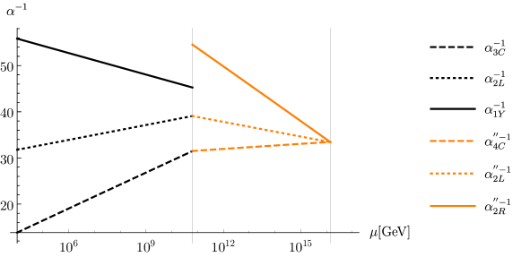
Figure 1: Running and gauge coupling unification in Model 1 in the case of minimal threshold corrections.

Figure 1 shows the predicted running of the gauge couplings for the case of minimal threshold corrections, in which all scalar masses are degenerate with the corresponding gauge boson masses.

Figure 2: Intermediate and unification scale for randomised scalar threshold corrections in Model 1. Only the large orange points are not excluded by our constraints. Points in blue are excluded by proton decay limits, points in black are excluded by the limits from black hole superradiance constraints. Points in green are allowed by black hole superradiance and proton decay, but forbidden by the chosen range of B-L breaking. The black cross indicates the minimal threshold case, i.e. the case when all scalar masses are degenerate and at the corresponding unification scales for which the running of the gauge couplings is illustrated in figure 1. We have performed the scan for 400 sets of initial conditions, 310 of which yielded unification of the gauge couplings.

Gauge coupling unification fixes the different scales in this case to

$$M_{\mathrm{U}}=M_{\mathrm{PQ}}=1.4\times 10^{16}\,\mathrm{GeV},\ \alpha_{\mathrm{U}}(M_{\mathrm{U}})^{-1}=33.6,\ M_{\mathrm{BL}}=6.3\times 10^{10}\,\mathrm{GeV}.$$ (113)

The unification scale is well above constraints from proton decay.

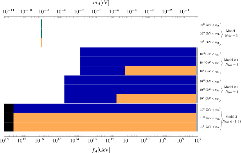
Figure 3: Possible ranges of the axion mass and decay constant consistent with gauge coupling unification in our models, for the case where all heavy scalars are degenerate at their various threshold scales. Regions in black are excluded by constraints from black hole superradiance, regions in blue by proton stability constraints. Regions in green are disfavoured depending on the allowed range of the B-L breaking scale. Regions in gray are excluded by stellar cooling constraints. The width of the region in Model 1 is exaggerated to make the bar visible. Note that for the Models 2.1, 2.2 and 3 the exclusion of the higher B-L breaking scales comes from an interplay of the proton stability constraint and the limit on $v_{\rm BL}$. In all these models, a higher B-L breaking scale corresponds to a lower GUT unification scale, which leads to an instability of the proton and is therefore excluded.

Exploiting the relation

$$M_{\mathrm{U}}=g_{U}v_{\rm U},$$ (114)

between the mass of the superheavy gauge bosons and the VEV $v_{\rm U}$ and the relation (93) between the axion decay constant and the VEVs, we obtain

$$f_{A}\simeq\frac{1}{3}\,v_{\rm U}=\frac{M_{\mathrm{U}}}{3g_{U}}=\frac{\sqrt{\alpha_{U}(M_{\mathrm{U}})^{-1}}}{3\sqrt{4\pi}}M_{\mathrm{U}}=7.7\times 10^{15}\,\mathrm{GeV},$$ (115)

yielding, via (26), an axion mass

$$m_{A}=7.4\times 10^{-10}\,\,\mathrm{eV}.$$ (116)

This result is illustrated in the first three lines of figure 3, which summarises our results for the case of vanishing threshold corrections.

As illustrated in figure 2 and as already pointed out in Dixit:1989ff , taking into account the possibility of scalar threshold corrections induces large uncertainties in the prediction of the GUT scale, which result in corresponding large uncertainties in the prediction of the axion mass. Including constraints from proton decay limits and the non-observation of black hole superradiance, the allowed range is

$$2.6\times 10^{15}\,\mathrm{GeV}<f_{A}<3.0\times 10^{17}\text{GeV},$$ (117)

$$1.9\times 10^{-11}\,\mathrm{eV}<m_{A}<2.2\times 10^{-9}\,\mathrm{eV}.$$

Finally, we have considered the various constraints imposed by the B-L breaking scale. As shown in figure 2, varying the allowed range of $v_{\mathrm{BL}}$ changes the viable range of $v_{\mathrm{PQ}}$and therefore of $f_{A}$. For $v_{\mathrm{BL}}>10^{11}(10^{13})\,\mathrm{GeV}$, the upper bound on $f_{A}$ is lowered to $1.0\times 10^{17}(3.5\times 10^{15})\,\mathrm{GeV}$. In the latter case, our random sample contains only two viable points (cf. figure 2).

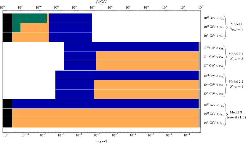
Figure 4: Possible ranges of the axion mass and decay constant consistent with gauge coupling unification in our models, for the case where scalar threshold corrections have been taken into account. Regions in black are excluded by constraints from black hole superradiance, regions in blue by proton stability constraints. Regions in green are disfavoured depending on the allowed range of the B-L breaking scale. Regions in gray are excluded by non-observation of excessive cooling of helium burning stars by axion emission.

These findings are summarised in the first three lines of figure 4.

5.2 Running with two intermediate scales

5.2.1 An extra multiplet

In the Model 2.1 described in (96), the requirement of gauge coupling unification does not sufficiently constrain the system of differential equations to uniquely fix both intermediate scales - we can only infer a relationship between the three unification scales $M_{\mathrm{PQ}},M_{\mathrm{BL}}$ and $M_{\mathrm{U}}$. We have calculated this relationship, and also imposed the aforementioned limits on the unification scale and on the B-L breaking scale.

Depending on which VEV is bigger, the RG running is different. In case B, i.e. $M_{\mathrm{PQ}}$<$M_{\mathrm{BL}}$, the Peccei-Quinn breaking VEV does not break any gauge symmetries, and thus it is unconstrained by the evolution. In this case, we have essentially a two-step breaking model, in which the two symmetry breaking scales $M_{\mathrm{U}}$ and $M_{\mathrm{BL}}$ are fixed. In case A, with $M_{\mathrm{PQ}}$>$M_{\mathrm{BL}}$, $v_{\mathrm{PQ}}$ breaks the $SU(2)_{R}$ gauge symmetry and is therefore constrained by the evolution.

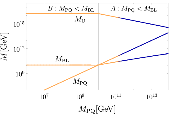
Figure 5: Relationship between the three unification scales for the Model 2.1 described in (96) in the case of minimal threshold corrections. The regions in blue are excluded by the non-observation of proton decay. In case B, $M_{\mathrm{PQ}}<M_{\mathrm{BL}}$, $M_{\mathrm{PQ}}$ is unconstrained - it can take any value, while the B-L breaking scale $M_{\mathrm{BL}}$ is fixed at $\sim 10^{10}\,\mathrm{GeV}$.

Both cases are indicated in figure 5.

In the case of minimal threshold corrections, in which all scalars are assumed to be degenerate in mass with the gauge bosons that get masses at the corresponding threshold scale, gauge coupling unification and limits from proton decay constrain the intermediate scale $M_{\mathrm{BL}}$ between

$$10^{10}\,\mathrm{GeV}\lesssim M_{\mathrm{BL}}\lesssim 2.3\times 10^{10}\,\mathrm{GeV}$$ (118)

and put an upper bound on $M_{\mathrm{PQ}}$ of order

$$M_{\mathrm{PQ}}<1.3\times 10^{11}\,\mathrm{GeV},$$ (119)

cf. figure 5.

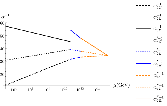
Figure 6: Running gauge couplings for $M_{\rm BL}=6.3\times 10^{10}\,\mathrm{GeV}$ in Model 2.1. The corresponding higher unifications scales are $M_{\rm PQ}=1.3\times 10^{12}\,\mathrm{GeV}$ and $M_{\rm U}=2.1\times 10^{15}\,\mathrm{GeV}$. Threshold corrections due to non-degenerate scalars are not included. Beta functions for this model are given in Appendix C.

An example of the evolution of the gauge couplings in this case is shown in figure 6. For completeness, let us also mention the special case in which the PQ and the B-L scales are taken to coincide , $M_{\mathrm{PQ}}=M_{\mathrm{BL}}$. We find in this case, for minimal threshold corrections,

$$M_{\mathrm{PQ}}=M_{\mathrm{BL}}=1.1\times 10^{10}\,\mathrm{GeV},\hskip 12.91663ptM_{\mathrm{U}}=1.6\times 10^{16}\,\mathrm{GeV}.$$ (120)

The upper limit (119) on $M_{\mathrm{PQ}}$ – derived by proton decay constraints in the case of minimal threshold corrections – can be turned into an upper limit on the axion decay constant and a corresponding lower limit on the axion mass as follows. Since $M_{\mathrm{PQ}}$ is the mass of the gauge bosons that become heavy by the $SU(2)_{R}\rightarrow U(1)_{R}$ breaking, we get

$$M_{\mathrm{PQ}}=g_{R}v_{\rm PQ}.$$ (121)

The corresponding limit on the axion mass follows straightforwardly from

$$f_{A} =\frac{1}{3}v_{\rm PQ}=\frac{M_{\mathrm{PQ}}}{3g_{R}}=\frac{M_{\mathrm{PQ}}}{3\sqrt{4\pi}}\sqrt{\alpha_{R}^{-1}}\,<\,1.4\times 10^{11}\,\,\mathrm{GeV}$$ (122)

$$m_{A} >4.1\times 10^{-5}\,\,\mathrm{eV}.$$

This limit is illustrated in lines 4 to 6 of figure 3. This constraint however is still subject to potentially large corrections from scalar threshold effects.

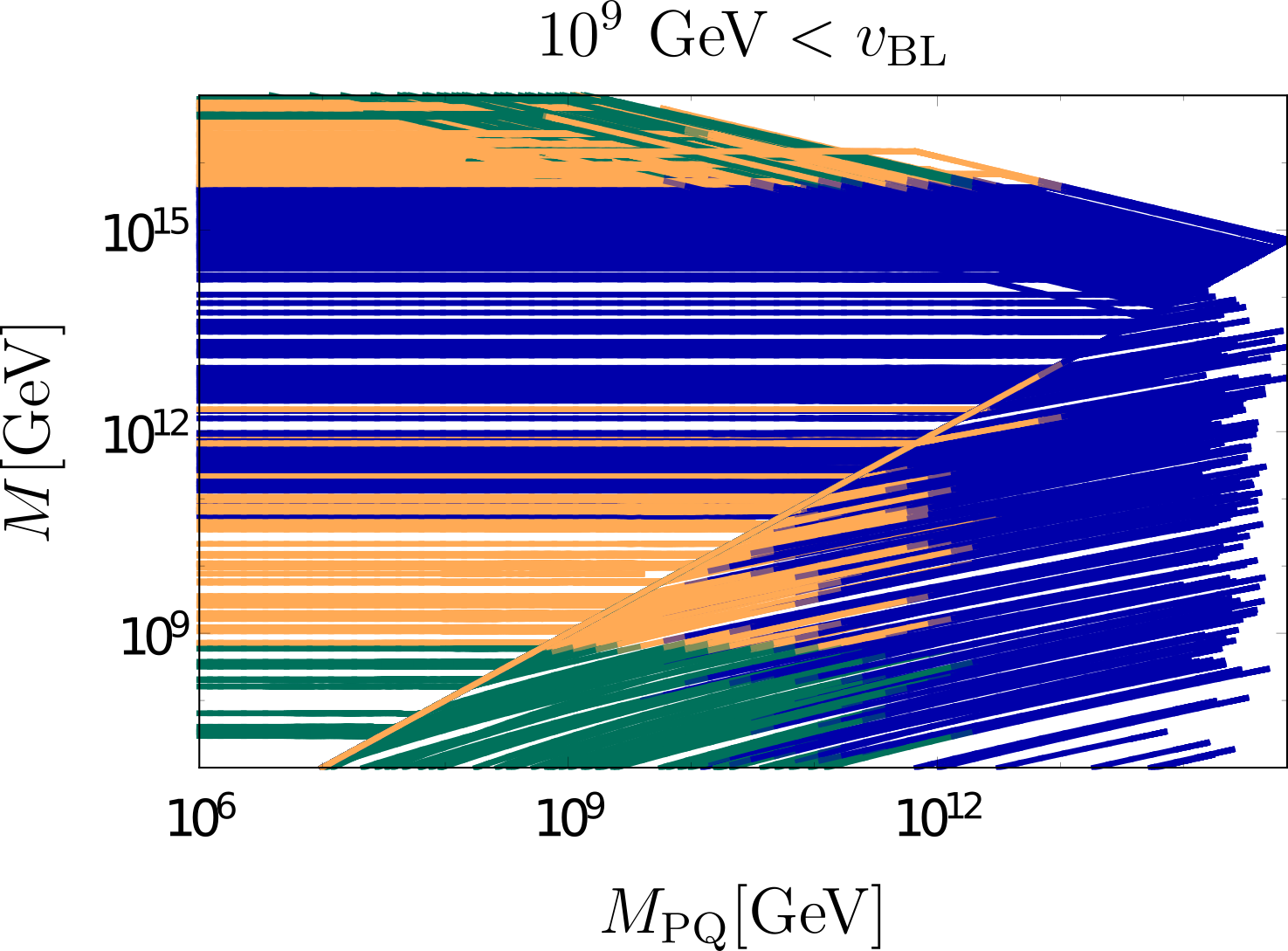
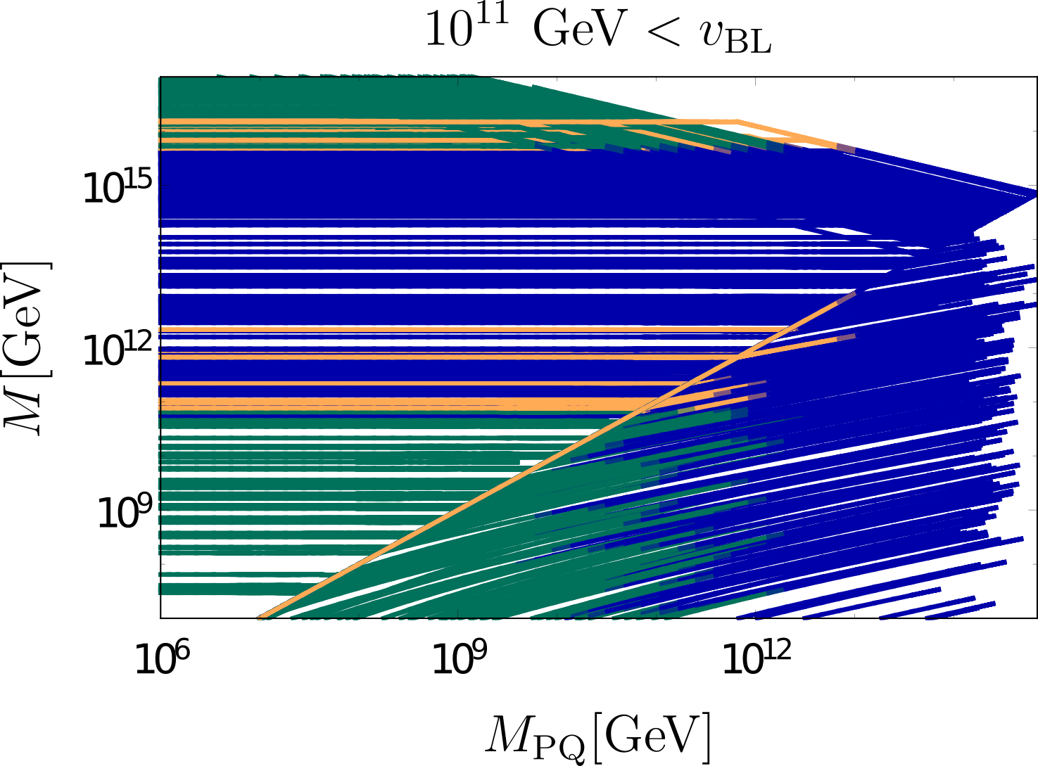
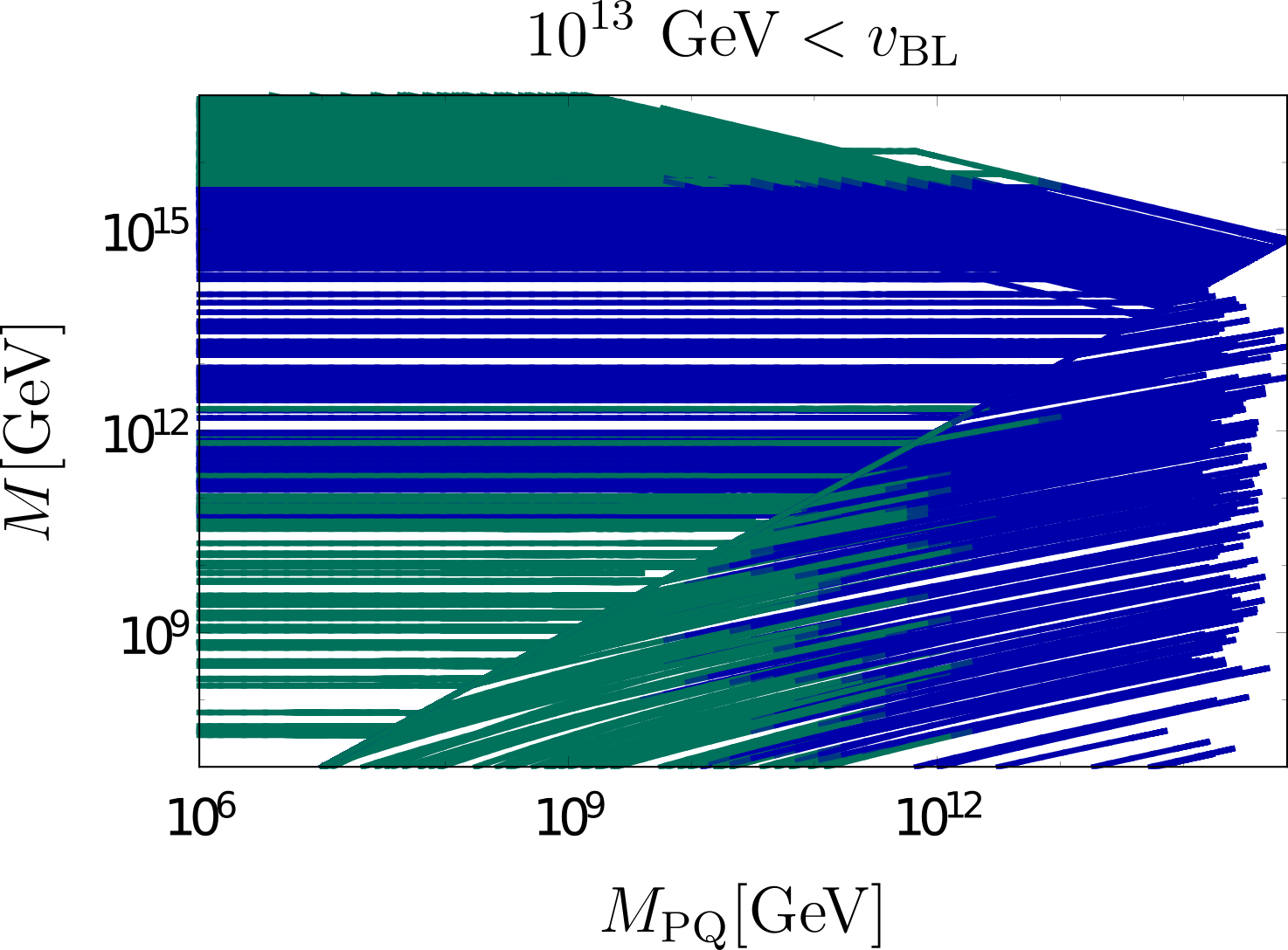
Figure 7: Intermediate scales $M_{\mathrm{PQ}}$ and $M_{\mathrm{BL}}$ and GUT-scale $M_{\mathrm{U}}$ for different threshold corrections in Model 2.1. Refer to figure 5 for clearer view of the different scales. The curves in blue are excluded by gauge-mediated proton decay limits, the curves in green by the limit on the B-L breaking scale. We have considered three different ranges of allowed B-L breaking scales. The threshold corrections are randomised in the following way: All scalars take masses among the values $\{\frac{1}{10},1,10\}$ times the corresponding threshold scale, where we have taken care not to make proton decay mediating scalars contained in the $(6,2,2)$ (Pati-Salam) multiplet light. We have chosen this discrete set of masses in order to focus on the largest possible corrections coming from the mass degeneracies. The scan was performed using 240 different sets of threshold corrections. Allowing the scalars to take masses in the whole interval $[\frac{1}{10},10]$ times the threshold scale, one could "fill the gaps" and find even more compatible solutions. These would however not significantly increase the allowed region of $M_{\rm PQ}$, whose upper and lower limits we are interested in.

In fact, in figure 7 we display the relation between the different unification scales –as in figure 5– but now for randomised scalar threshold corrections for different ranges of $v_{\rm BL}$. Obviously, the threshold corrections can increase the bound on $M_{\mathrm{PQ}}$ and thus on $f_{A}$. For $10^{9}(10^{11})\,\mathrm{GeV}<v_{\mathrm{BL}}<10^{15}\,\mathrm{GeV}$, we get $f_{A}<6.7\times 10^{12}\,\mathrm{GeV}$ and $m_{A}>8.5\times 10^{-7}\,\mathrm{eV}$, while for $10^{13}\,\mathrm{GeV}<v_{\mathrm{BL}}<10^{15}\,\mathrm{GeV}$ no allowed range of $f_{A}$ remains - in this case, the model is excluded. These findings are summarised in lines 4 to 6 of figure 4.

5.2.2 An extra multiplet, and additional fermions

Model 2.2 with PQ charges given in (101) contains additional quarks which acquire masses at the scale $M_{\mathrm{PQ}}$. Above $M_{\mathrm{PQ}}$, they contribute to the running of the coupling constants (cf. Appendix C). Correspondingly, in this model we obtain a relation between $M_{\mathrm{PQ}}$ and $M_{\mathrm{BL}}$ even in the case where $M_{\mathrm{PQ}}$ does not break a gauge symmetry.

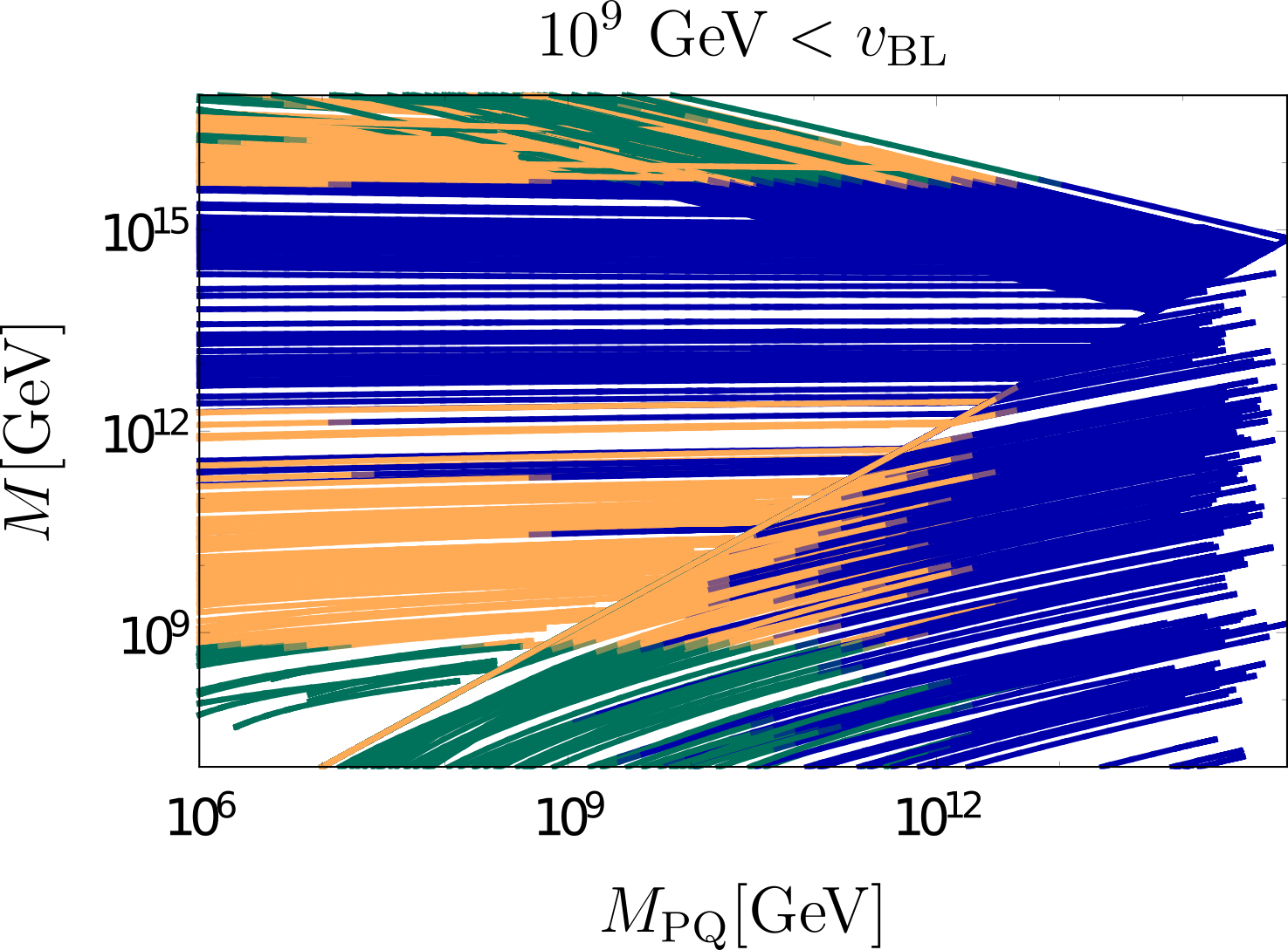
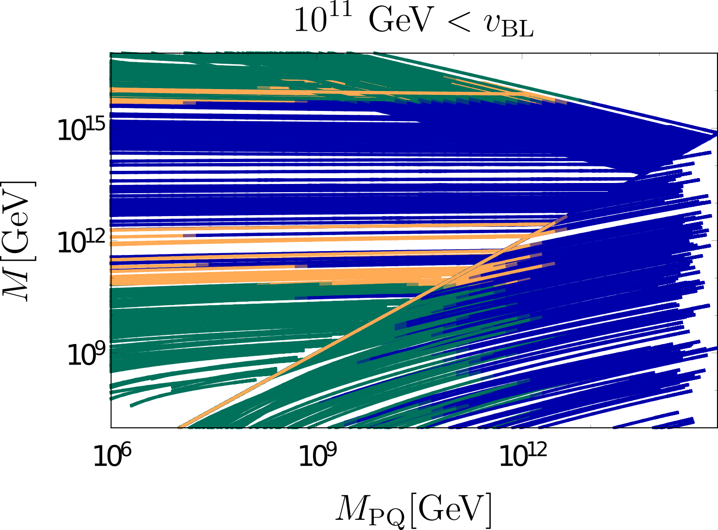
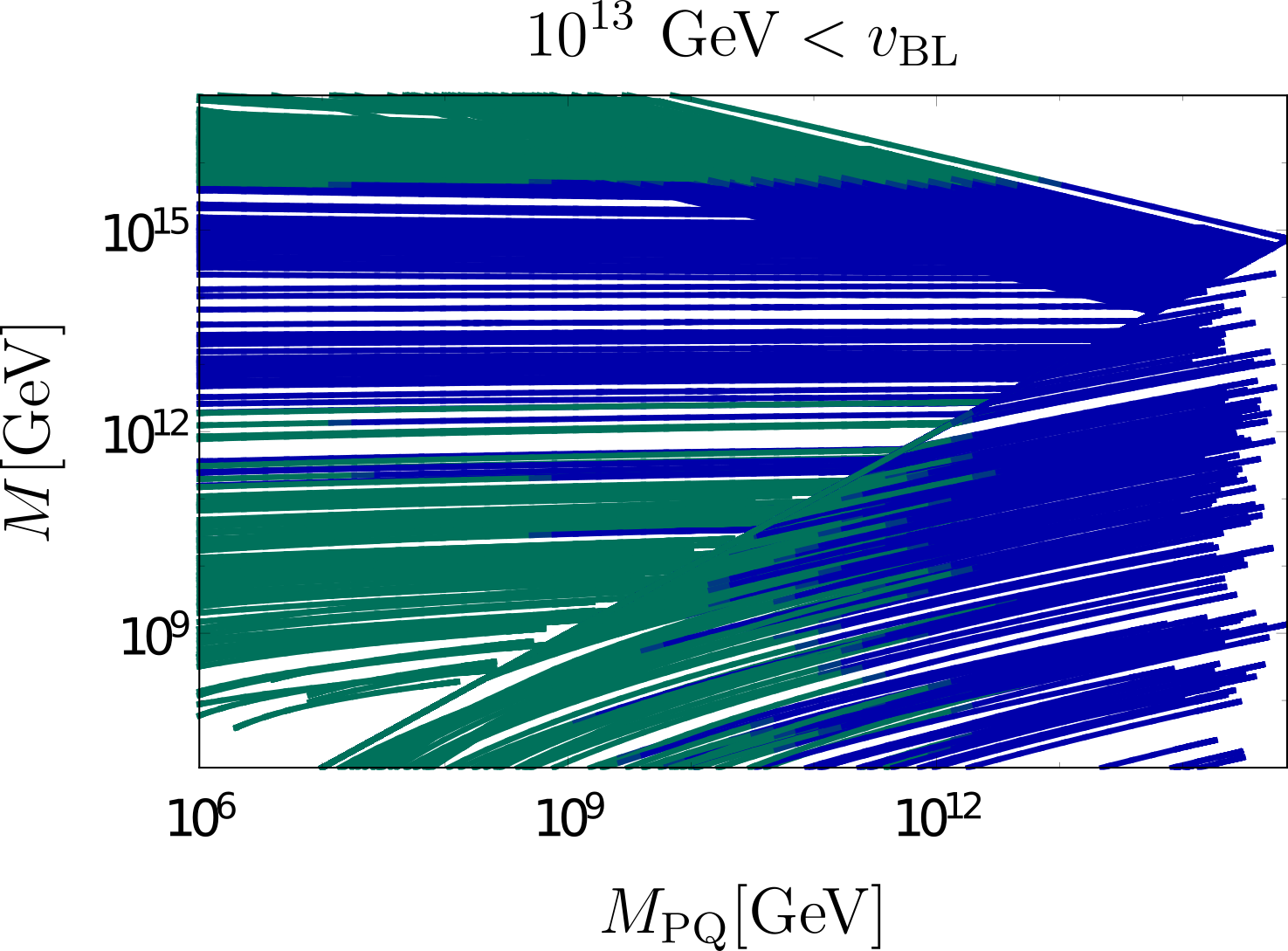
Figure 8: Intermediate scales $M_{\mathrm{PQ}}$ and $M_{\mathrm{BL}}$ and GUT-scale $M_{\mathrm{U}}$ for Model 2.2 for different threshold corrections. The curves in blue are excluded by gauge-mediated proton decay limits, the curves in green by the limit on the B-L breaking scale. We have considered three different ranges of allowed B-L breaking scales. The threshold corrections are randomised in the following way: All scalars take masses among the values $\{\frac{1}{10},1,10\}$ times the corresponding threshold scale, where we have taken care not to make proton decay mediating scalars contained in the $(6,2,2)$ (Pati-Salam) multiplet light.

The corresponding plots are shown in figure 8. After constraining the B-L breaking scale we obtain an upper limit on the axion mass and decay constant in this model. The minimal threshold case is only allowed if $M_{\mathrm{BL}}$ can be as low as $10^{9}\,\mathrm{GeV}$, in this case the maximal allowed $f_{A}$ is $4.2\times 10^{11}\,\mathrm{GeV}$ – this is also shown in lines 7 to 9 of figure 3.

Including all threshold corrections in our random sample, for $10^{9}(10^{11})\,\mathrm{GeV}<v_{\mathrm{BL}}<10^{15}\,\mathrm{GeV}$, $f_{A}$ is constrained to be smaller than $8.6\times 10^{12}\,\mathrm{GeV}$. For $10^{13}\,\mathrm{GeV}<v_{\mathrm{BL}}<10^{15}\,\mathrm{GeV}$, no viable solutions were found in the sample - the model is strongly disfavoured in this case. The results on the axion decay constant are summarised for this model in lines 7 to 9 of figure 4.

5.3 Models with a scalar singlet

In the simplest Model 3.1, described in (109), the Peccei-Quinn breaking is driven by a scalar singlet and the axion mass is unconstrained, cf. line 12 in figure 4. There is no relation between the PQ breaking scale and the two other scales. The possible ranges for $M_{\mathrm{U}}$ and $M_{\mathrm{BL}}$ however can be read from figure 2 –the extra scalar singlet in this model does not change the running. Also in this model a lower B-L breaking scale is preferred, and the model is excluded if $v_{\rm BL}>10^{13}\,\mathrm{GeV}$ is imposed.

If, however, we employ the mechanism of reference Lazarides:1982tw to reduce the domain wall number and introduce additional heavy fermions (Model 3.2, (110)), one has to account for how the latter change the running of the gauge couplings above the scale $M_{\rm PQ}$ at which they acquire their masses, if $M_{\rm PQ}<M_{\rm U}$.

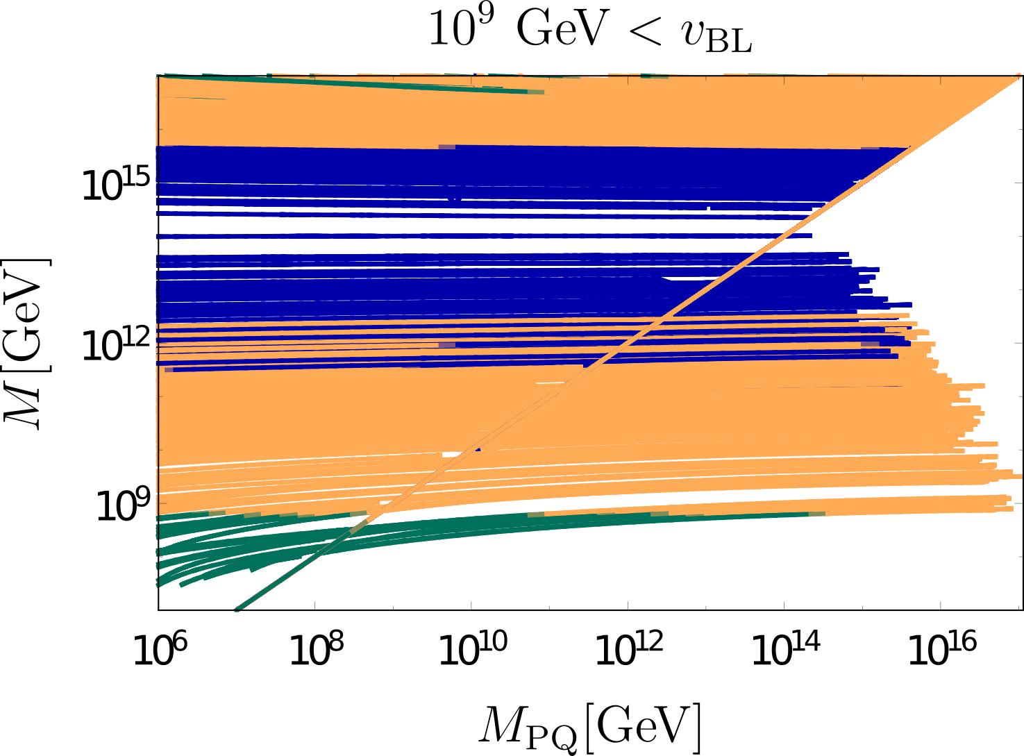
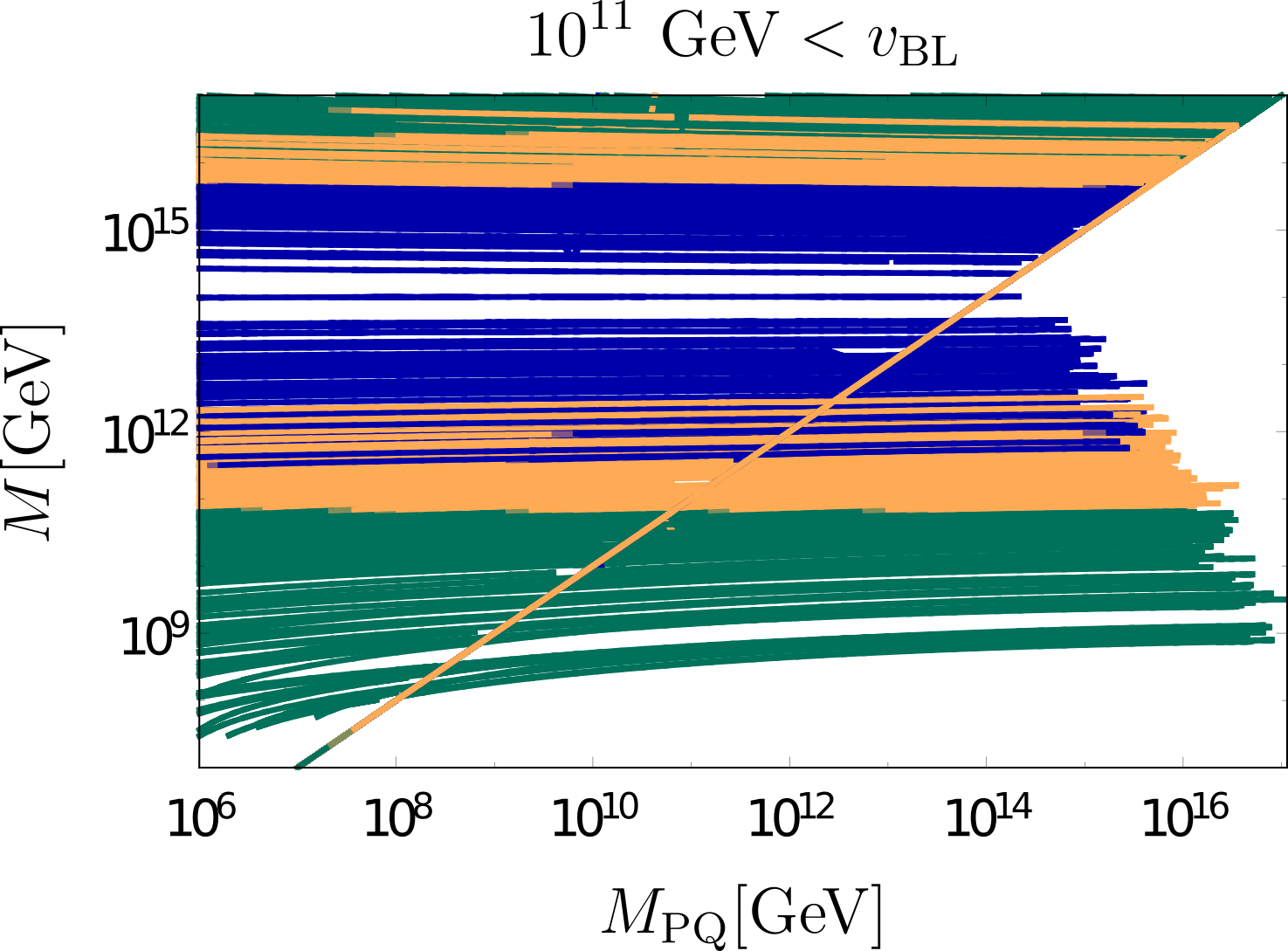
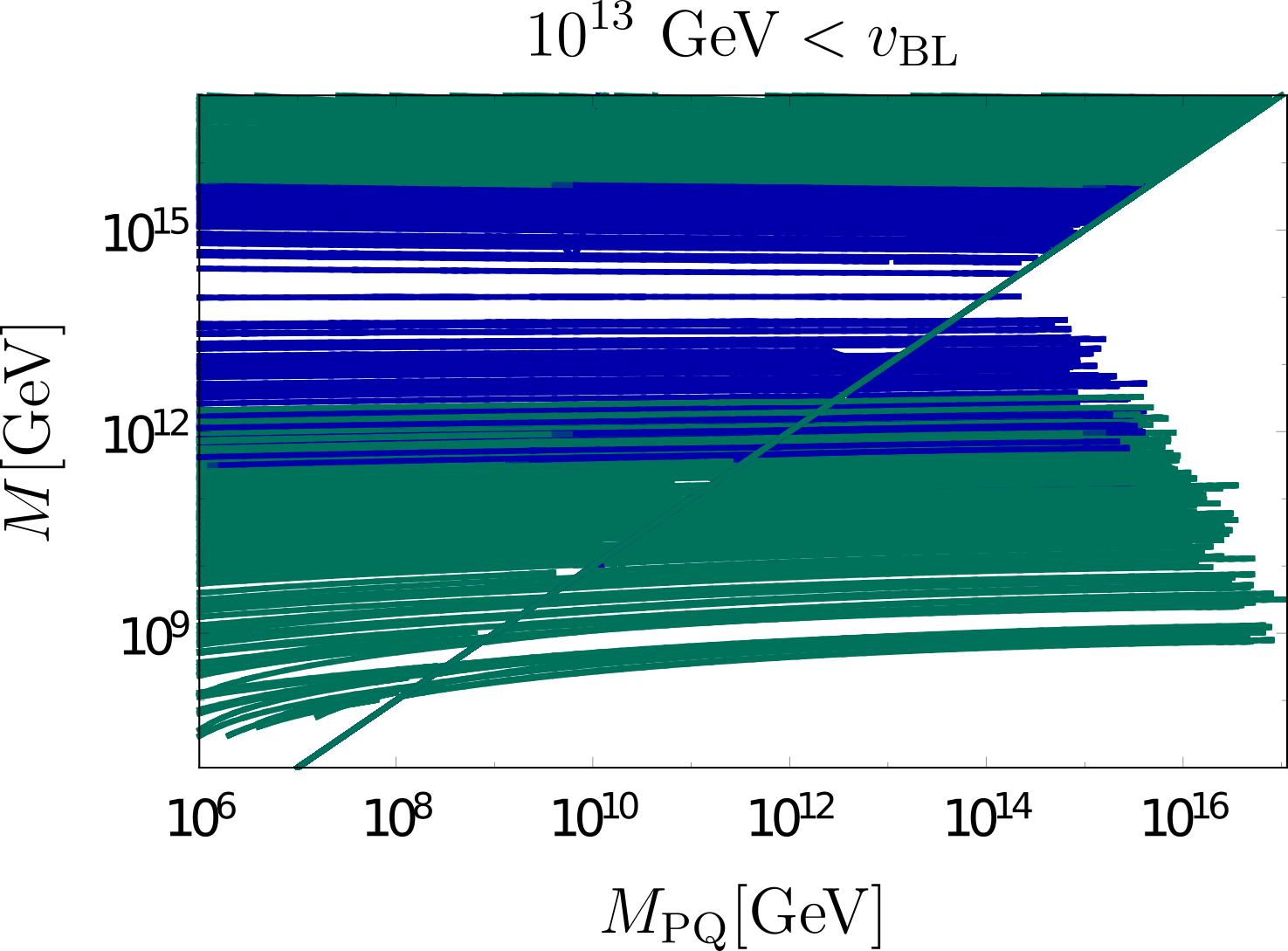
Figure 9: Intermediate scales $M_{\mathrm{PQ}}$ and $M_{\mathrm{BL}}$ and GUT-scale $M_{\mathrm{U}}$ for Model 3.2 for different threshold corrections. The curves in blue are excluded by gauge-mediated proton decay limits, the curves in green by the limit on the B-L breaking scale. We have considered three different ranges of allowed B-L breaking scales. The threshold corrections are randomised in the following way: All scalars take masses among the values $\{\frac{1}{5},1,5\}$ times the corresponding threshold scale, where we have taken care not to make proton decay mediating scalars light. We have reduced the range of possible threshold corrections since the bigger range did not yield enough viable solutions.

Correspondingly we obtain a relation between the scales $M_{\mathrm{U}}$, $M_{\mathrm{PQ}}$ and $M_{\mathrm{BL}}$ also in this model. However, this dependence –plotted in figure 9 for different sets of threshold corrections– is very weak, and the additional fermions do not change the beta functions enough to introduce additional constraints. We have verifed that the model is still allowed in the entire parameter space of $v_{\rm PQ}$.

For $M_{\rm PQ}>M_{\rm U}$, the extra fermions are integrated out above the GUT scale and do not change the running of the three gauge couplings. This case is always allowed, as long as the model without the additional fermions is not ruled out. The only constraint on both Models 3.1 and 3.2 – which we summarise as Model 3– comes then from the B-L breaking scale. For degenerate scalars at the thresholds, we need to allow for $v_{\rm BL}$ as low as $10^{9}\,\mathrm{GeV}$, as indicated in lines 10 to 12 of figure 3. If we allow variations in the masses of the heavy scalars, values of $v_{\rm BL}$ of order $10^{11}-10^{12}\,\mathrm{GeV}$ are still allowed. For $v_{\rm BL}>10^{13}\,\mathrm{GeV}$, Model 3 is excluded. This is illustrated in in lines 10 to 12 of figure 4.

5.4 Dependence on the proton lifetime

In our analysis we are dealing with three different scales, none of which have been observed so far. Apart from the axion mass, one could also hope to constrain the unification scale in the future by detecting proton decay. The projected sensitivity of the Hyper-Kamiokande Cherenkov detector to the channel $p\rightarrow e^{+}\pi^{0}$ after 10 years of measurement is $1.3\times 10^{35}{\rm yr}$ at $90\%$CL Abe:2014oxa . Assuming that proton decay is observed during the first decade of Hyper-Kamiokande, we can place further (hypothetical) constraints on the axion decay constant in each of our models. In figure 10 we illustrate how an upper bound

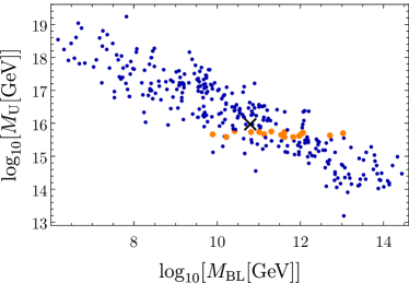
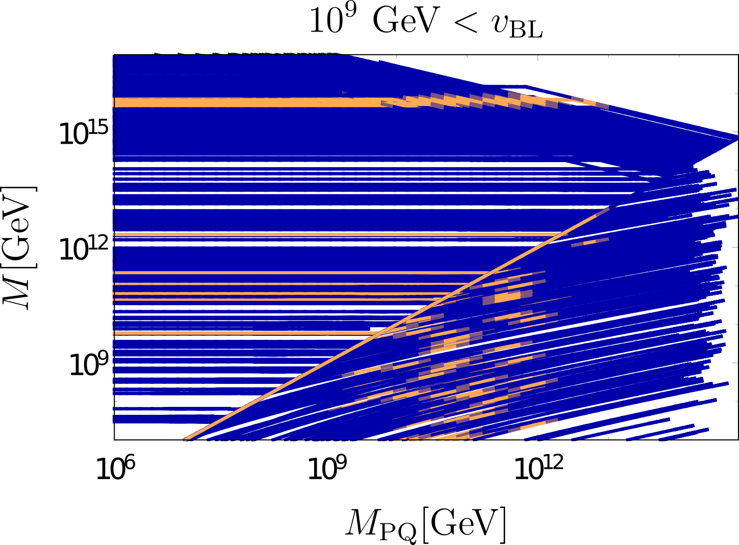
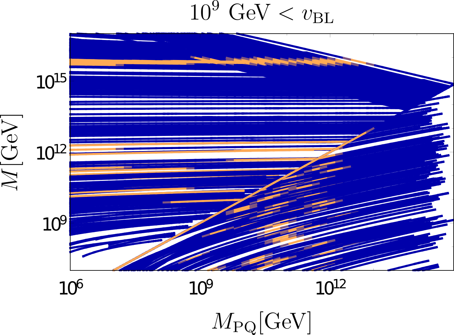
Figure 10: Intermediate and unification scale for randomised scalar threshold corrections in Models 1 (top), 2.1 (bottom left) and 2.2 (bottom right) including the limit coming from a hypothetical observation of proton decay at Hyper-Kamiokande. Only the orange points/regions are not excluded by the constrained proton lifetime. For models 2.1 and 2.2, the threshold corrections induce large uncertainties in the viable $f_{A}$ ranges even in the case where the unification scale is known.

on the proton decay scale constrains the scale of Peccei-Quinn breaking and ergo the axion decay constant and mass. We make a naive analysis and assume that proton decay is only mediated by the heavy gauge bosons. As a lower bound for the proton lifetime we use the present limit $1.6\times 10^{34}{\rm yr}$ Miura:2016krn . As shown in figure 11, an observation of proton decay is very constraining only for our Model 1 –here we obtain $2.6\times 10^{15}\,\mathrm{GeV}<f_{A}<4.0\times 10^{15}\,\mathrm{GeV}$- , while in the other models the allowed ranges of $f_{A}$ are still rather large.

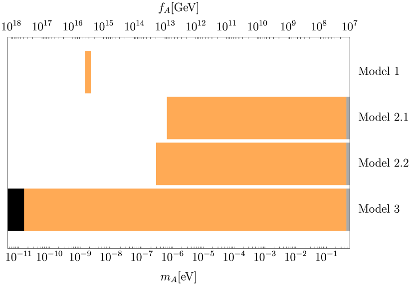
Figure 11: Viable ranges of $f_{A}$ in the hypothetical case of a known proton lifetime between $1.6\times 10^{34}$ and $1.3\times 10^{35}$ years. Allowed regions are plotted in orange. Regions in black are excluded from black hole superradiance constraints, regions in gray from the non-observation of excessive stellar cooling.

6 Summary and discussion

We have analysed various non-supersymmetric Grand Unified $SO(10)\times U(1)_{\rm PQ}$ models for their predictions on the axion mass, the domain wall number, and the low-energy couplings to SM particles. The basic field content of all the considered models consisted of three spinorial $16_{F}$ representations of $SO(10)$ representing the fermionic matter content and three Higgs representations: $210_{H}$, $\overline{126}_{H}$ and $10_{H}$, see table 5.

$$\begin{array}[]{|l|c|c|c|c|c|c|c||c|}\hline\cr&16_{F}&\overline{126}_{H}&10_{H}&210_{H}&45_{H}&S&10_{F}&N_{\rm DW}\\ \hline\cr{\bf Model\ 1}&1&-2&-2&4&-&-&-&3\\ \hline\cr{\bf Model\ 2.1}&1&-2&-2&0&4&-&-&3\\ \hline\cr{\bf Model\ 2.2}&1&-2&-2&0&4&-&-2&1\\ \hline\cr{\bf Model\ 3.1}&1&-2&-2&0&-&4&-&3\\ \hline\cr{\bf Model\ 3.2}&1&-2&-2&0&-&4&-2&1\\ \hline\cr\end{array}$$

Table 5: Field content, PQ charge assignments, and resulting domain wall number $N_{\rm DW}$ in the various $SO(10)\times U(1)_{\rm PQ}$ models considered in this paper.

The latter have been assumed to take VEVs in such a way that $SO(10)$ is broken along the symmetry breaking chain

$$SO(10) \stackrel{{\scriptstyle M_{\rm U}-210_{H}}}{{\longrightarrow}} 4_{C}\,2_{L}\,2_{R}\ \stackrel{{\scriptstyle M_{\rm BL}-\overline{126}_{H}}}{{\longrightarrow}}3_{C}\,2_{L}\,1_{Y}\ \stackrel{{\scriptstyle M_{Z}-10_{H}}}{{\longrightarrow}}\ 3_{C}\,1_{\rm em}\,.$$

In some of the models, this basic field content was extended by further scalar and fermion representations. This includes an additional scalar in the $45_{H}$, in which case we have considered a further symmetry breaking chain,

$$SO(10) \stackrel{{\scriptstyle M_{\rm U}-210_{H}}}{{\longrightarrow}}4_{C}\,2_{L}\,2_{R}\,\stackrel{{\scriptstyle M_{\rm PQ}-45_{H}}}{{\longrightarrow}}4_{C}\,2_{L}\,1_{R}\,\stackrel{{\scriptstyle M_{\rm BL}-126_{H}}}{{\longrightarrow}}3_{C}\,2_{L}\,1_{Y}\,\stackrel{{\scriptstyle M_{Z}-10_{H}}}{{\longrightarrow}}\ 3_{C}\,1_{\rm em}.$$

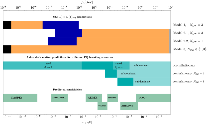
Figure 12: Possible ranges of the axion mass and decay constant consistent with gauge coupling unification in our four models. Regions in black are excluded by constraints from black hole superradiance, regions in dark blue by proton stability constraints. Regions in gray are excluded by stellar cooling constraints from horizontal branch stars in globular clusters Ayala:2014pea . For comparison, we show also the mass regions preferred by axion dark matter (DM) (lines 5 to 7), cf. Saikawa:2017lzn . Here, the dark regions indicate the ranges where the axion can make up the main part of the observed DM, with the possibility of fine tuning the initial misalignment angle in the scenario where the PQ symmetry is broken before the end of inflation and not restored thereafter (pre-inflationary PQ symmetry breaking scenario). In the light regions, axions could still be DM, but not the dominant part. The remaining regions are not allowed - axions in this mass range would be overabundant. Note that the region in the $N_{\rm DW}=3$ case has been derived under the assumption that the PQ symmetry is protected by a discrete symmetry, so that Planck scale suppressed PQ violating operators are allowed at dimension 10 or higher Ringwald:2015dsf . In the last two lines the projected sensitivities of various experiments are indicated Budker:2013hfa ; Stern:2016bbw ; Chung:2016ysi ; Kahn:2016aff ; TheMADMAXWorkingGroup:2016hpc ; Arvanitaki:2014dfa ; Armengaud:2014gea ; Giannotti:2017hny .

In all models one can choose a basis of fermion fields for which the phenomenologically most important couplings to photons ($\gamma$), electrons ($f=e$), protons ($f=p$) and neutrons ($f=n$) read, at energies lower than $\Lambda_{\rm QCD}$,

$${\cal L}=\frac{1}{2}\partial_{\mu}A\partial^{\mu}A-\frac{1}{2}m_{A}^{2}A^{2}+\frac{\alpha}{8\pi}\,\frac{C_{A\gamma}}{f_{A}}\,A\,F_{\mu\nu}{\tilde{F}}^{\mu\nu}-\frac{1}{2}\,\frac{C_{Af}}{f_{A}}\,\partial_{\mu}A\ \overline{\Psi}_{f}\gamma^{\mu}\gamma_{5}\Psi_{f}\,,$$ (123)

with

$$m_{A}={57.0(7)\,\left(\frac{10^{11}\rm GeV}{f_{A}}\right)\mu\text{eV},}$$ (124)

and with the couplings $C_{Ax}$ given by

$$C_{A\gamma}=\frac{8}{3}-1.92(4)\,,\qquad C_{Ae}=\frac{1}{N_{\rm DW}}\sin^{2}\beta\,,$$

$$C_{Ap}=-0.47(3)+\frac{3}{N_{\rm DW}}[0.29\cos^{2}\beta-0.15\sin^{2}\beta\pm 0.02]\,,$$ (125)

$$C_{An}=-0.02(3)+\frac{3}{N_{\rm DW}}[-0.14\cos^{2}\beta+0.28\sin^{2}\beta\pm 0.02]\,,$$

where $\tan^{2}\beta=((v_{u}^{10})^{2}+(v_{u}^{126})^{2})/((v_{d}^{10})^{2}+(v_{d}^{126})^{2})$, and $N_{\rm DW}$ is the domain-wall number, which in the models considered is either 3 or 1. For $N_{\rm DW}=3$ one recovers the results for the DFSZ axion Zhitnitsky:1980tq ; Dine:1981rt ; Srednicki:1985xd ; diCortona:2015ldu , although the microscopic origin of the parameter $\beta$ differs (as it is determined by the VEVs of four Higgses, as opposed to two in DFSZ models). The fermion fields for which the above interactions are valid are obtained after special axion-dependent rotations of the fermion fields that carry charges under the global symmetry ${\rm PQ}_{\rm phys}$ compatible with the GUT symmetry. These fermion rotations do not act in the same way over all the components of the $16_{F}$ multiplets, and thus will “hide” the GUT symmetry, and moreover modify the axion couplings to the weak gauge bosons. A possible measurement of the latter couplings would open up the possibility of recovering the GUT compatible charges under ${\rm PQ}_{\rm phys}$, and discriminate these models from e.g. simpler DFSZ scenarios.

The overall phenomenologically viable range in the axion decay constant of these models spans a very wide range, $10^{7}\,\,\mathrm{GeV}\lesssim f_{A}\lesssim 10^{17}\,\,\mathrm{GeV}$, corresponding to an axion mass $m_{A}$ between $10^{-10}$ eV and $10^{-1}$ eV (see the orange regions in figure 12). These predictions survive constraints from gauge coupling unification, from black hole superradiance (black), from proton decay (blue), and stellar cooling (gray). The features of the different models are summarised next.

Model 1 – employing just the basic field content mentioned above and assuming that all these fields are charged under the PQ symmetry, cf. equation (86) and table 5 – appears to be most predictive. In fact, we infer from the first line in figure 12 that the aforementioned phenomenological constraints result in an axion parameter region

$$2.6\times 10^{15}\,\mathrm{GeV}<f_{A}<3.0\times 10^{17}\text{GeV},\hskip 12.91663pt1.9\times 10^{-11}\,\mathrm{eV}<m_{A}<2.2\times 10^{-9}\,\mathrm{eV},$$ (126)

if we allow the seesaw scale to get as low as $v_{\rm BL}\simeq 10^{9}\,\,\mathrm{GeV}$. The allowed axion mass range moves towards the upper end, $m_{A}\simeq 2.2\times 10^{-9}\,\,\mathrm{eV}$, if we restrict the seesaw scale to higher values, $v_{\rm BL}\gtrsim 10^{13}\,\,\mathrm{GeV}$, cf. figure 4 (first and second line).

The small axion mass predicted in Model 1 implies that the PQ symmetry has to be broken before and during inflation and must not be restored thereafter Borsanyi:2016ksw (pre-inflationary PQ symmetry breaking scenario). In fact, in the opposite case (post-inflationary PQ symmetry breaking scenario), the axion mass is bounded from below by about $23\,\mu$eV Borsanyi:2016ksw ; Klaer:2017ond , cf. figure 12. In order for axion cold dark matter not to become overabundant, the initial value of the axion field in the causally connected patch which contains the present universe had to be small, $10^{-3}\lesssim|\theta_{i}|=|A(t_{i})/f_{A}|\lesssim 10^{-2}$ Borsanyi:2016ksw . Furthermore, the Hubble expansion rate during inflation must have been small, $H_{I}\lesssim 10^{9}\,\,\mathrm{GeV}$, to avoid constraints from the non-observation of traces of isocurvature fluctuations in the cosmic microwave background radiation Turner:1990uz ; Beltran:2006sq ; Hertzberg:2008wr ; Hamann:2009yf . The latter constraint disqualifies Model 1 as a possible GUT SMASH candidate, since in Higgs portal inflation the Hubble expansion rate during inflation is of order $10^{13}\,\,\mathrm{GeV}\lesssim H_{I}\lesssim 10^{14}\,\,\mathrm{GeV}$ Ballesteros:2016xej .

Remarkably, the predicted axion mass range of Model 1 will be probed in the upcoming decade by the CASPEr experiment Budker:2013hfa , cf. figure 12, which aims to detect directly axion dark matter by precision nuclear magnetic resonance techniques. If successful and interpreted in terms of Model 1, one may translate, via (115), the measurement of the axion mass into an indirect determination of the mass of the superheavy gauge bosons, i.e. the unification scale,

$$M_{\mathrm{U}}\simeq 3g_{U}\sqrt{\chi}/m_{A},$$ (127)

where $\chi$ is the topological susceptibility in QCD, $\chi=[75.6(1.8)(0.9){\rm MeV}]^{4}$ diCortona:2015ldu ; Borsanyi:2016ksw . The unification scale can be probed complementarily by the next generation of experiments searching for signatures of proton decay, such as Hyper-Kamiokande Abe:2011ts or DUNE Kemp:2017kbm .

Models featuring an axion with a larger mass, $m_{A}\gtrsim 23\,\mu$eV, compatible with the post-inflationary PQ symmetry breaking scenario, can only be obtained if the $210_{H}$ responsible for the first gauge symmetry breaking at $M_{\mathrm{U}}$ has no PQ charge. But in addition – as emphasised already in references Holman:1982tb ; Bajc:2005zf – the scalar sector has to be extended by yet another PQ charged field obtaining a VEV. Otherwise the axion decay constant is predicted to be as low as the electroweak scale, which is firmly excluded by laboratory experiments and stellar astrophysics. Correspondingly, we considered also models which have additional scalar fields such as a PQ charged $45_{H}$ (Models 2.1 and 2.2) or a PQ charged $SO(10)$ singlet complex scalar field $S$ (Models 3.1 and 3.2), cf. table 5. Crucially, in these extended models, the PQ symmetry breaking scale $v_{\rm PQ}$ and the seesaw scale $v_{\rm BL}$ are independent parameters – in fact, the axion field has to be orthogonal to the Goldstone field which is eaten by the gauge bosons getting mass by B-L breaking. This is different in the original SMASH model Ballesteros:2016euj ; Ballesteros:2016xej , where the PQ symmetry is at the same time also a B-L symmetry.

Model 2.1 features PQ charges for the $16_{F}$, $\overline{126}_{H}$ and $10_{H}$ multiplets and an additional PQ charged $45_{H}$, cf. (96) and table 5. The range in the axion decay-constant/mass is predicted to be quite distinct from the one of Model 1, see figure 12. Just accounting for gauge coupling unification with scalar threshold corrections, we have found an upper bound on the decay-constant $f_{A}<4.0\times 10^{14}\,\,\mathrm{GeV}$, and a corresponding lower bound on the axion mass, $m_{A}>1.4\times 10^{-8}\,{\rm eV}$. Imposing in addition constraints from proton decay, the upper limit on $f_{A}$ comes further down, while constraints on the photon coupling from stellar cooling introduce also a lower limit on $f_{A}$,

$$1.3\times 10^{7}\,\mathrm{GeV}<f_{A}<6.7\times 10^{12}\text{GeV},\hskip 12.91663pt8.5\times 10^{-7}\,\mathrm{eV}<m_{A}<0.5\,\,\mathrm{eV}.$$ (128)

Furthermore, the model features an upper limit on the scale of B-L breaking: $v_{\rm BL}<10^{13}\,\mathrm{GeV}$, cf. figure 4.

In this model, both the pre-inflationary as well as the post-inflationary PQ symmetry breaking scenarios are possible, see figure 12. As far as the latter case is concerned, it is important to note that the possibly inherent domain wall problem can be circumvented if the PQ symmetry is only a low energy remnant of an exact discrete symmetry, so that Planck scale suppressed PQ violating operators – which have been argued to be induced in any case by quantum gravity effects Ghigna:1992iv ; Barr:1992qq ; Kamionkowski:1992mf ; Holman:1992us , and which render string-wall systems with $N_{\rm DW}>1$ unstable – occur at dimension ten Ringwald:2015dsf .

$$\begin{array}[]{|c|c|c|c|c|c|}\hline\cr&16_{F}&10_{H}&\overline{126}_{H}&45_{H}&S\\ \hline\cr\text{ Model 2.1}&-\frac{1}{40}&\frac{1}{20}&\frac{1}{20}&-\frac{1}{10}&-\\ \hline\cr\text{ Model 3.1}&-\frac{1}{40}&\frac{1}{20}&\frac{1}{20}&-&-\frac{1}{10}\\ \hline\cr\end{array}$$

Table 6: Charges of the fermionic and scalar fields under a PQ-protecting discrete $\mathcal{Z}_{40}$ symmetry for Models 2.1 and 3.1. The lowest dimensional PQ violating operators allowed by these symmetries are $45_{H}^{10}$ for Model 2.1 and $S^{10}$ for Model 3.1.

In this case, the preferred mass range for dark matter is a bit higher than the one singled out in the post-inflationary $N_{\rm DW}=1$ scenario. In particular, for $N_{\rm DW}=3$, as in Model 2.1, it is given by $0.18\,{\rm meV}\lesssim m_{A}\lesssim 2.0\,{\rm meV}$, cf. figure 12. Intriguingly, for $m_{A}={\mathcal{O}}(10)$ meV and $\tan\beta\gtrsim 0.3$, the axion in this model may explain at the same time recently observed stellar cooling excesses observed from helium burning stars, red giants and white dwarfs Giannotti:2017hny .

Fortunately, there are a number of running (ADMX Stern:2016bbw , HAYSTAC Brubaker:2016ktl , ORGAN McAllister:2017lkb ), presently being assembled (CULTASK Chung:2016ysi , QUAX Barbieri:2016vwg ), or planned (ABRACADABRA Kahn:2016aff , KLASH Alesini:2017ifp , MADMAX TheMADMAXWorkingGroup:2016hpc , ORPHEUS Rybka:2014cya ) axion dark matter experiments, which cover a large portion of the mass range of interest for axion dark matter in the pre-inflationary PQ symmetry scenario in Model 2.1, see figure 12. Furthermore, in the meV mass range of interest for the post-inflationary PQ symmetry breaking scenario, the model can be probed by the presently being build fifth force experiment ARIADNE Arvanitaki:2014dfa and the proposed helioscope IAXO Armengaud:2014gea , cf. figure 12.

Model 2.2 adds to the field content of Model 2.1 two PQ charged vector representations $10_{F}$ of $SO(10)$, getting their mass from the $45_{H}$ and cancelling two units of the domain wall number. Correspondingly, Model 2.2 has no domain wall problem whatsoever. Allowing $v_{\rm BL}$ to be as small as $10^{9}\,\mathrm{GeV}$, the allowed mass range in this model is very similar to the one of Model 2.1. Taking into account additional limits from gauge coupling unification, proton decay and the limit from stellar cooling, the preferred ranges in this model are

$$1.3\times 10^{7}\,\mathrm{GeV}<f_{A}<1.5\times 10^{13}\,\mathrm{GeV},\hskip 12.91663pt3.8\times 10^{-7}\,\mathrm{eV}<m_{A}<0.5\,\,\mathrm{eV}.$$ (129)

This model can be probed by the same experiments as Model 2.1. Similar to Model 2.1, this model allows for axions in the post-inflationary DM window. Remarkably, the model features a second potential DM candidate: the lightest stable combination of the additional fermions Mambrini:2015vna ; Nagata:2015dma ; Arbelaez:2015ila ; Boucenna:2015sdg . Therefore we do not need to insist on the axion being $100\%$ of the observed dark matter and can allow for bigger axion masses (cf. the region labelled "subdominant" in the $N_{\rm DW}=1$ bar of figure 12).

Model 3.1 contains PQ-charged fermions in the $16_{F}$ representation, as well as PQ charged scalars in the $10_{H}$, $\overline{126}_{H}$ and a singlet $S$. The axion decay constant in this model is set by the VEV of the scalars singlet. It is a free parameter not constrained by gauge coupling unification, since it does not break any gauge symmetries. In a sense, Model 3.1 is the most minimal GUT model with an invisible axion with decay constant possibly in the intermediate range between the electroweak scale and the unification scale, see figure 12. Similar to Model 2.1, its possible domain wall problem in the post-inflationary symmetry breaking case can be avoided if the PQ symmetry is only an accidental symmetry of a discrete symmetry which forbids PQ-violating operators up to dimension 10. For an example of such a discrete symmetry, we refer to table 6.

Model 3.2 adds to the field content of Model 3.1 two vectorial $10_{F}$ representations of fermions getting their masses by the VEV $v_{S}$ of the singlet $S$. Despite the fact that the fermions affect the running of gauge couplings at scales above $v_{S}$, we found that, as in Model 3.1, the axion decay constant cannot be constrained by the running of the gauge coupling. Both models 3.1 and 3.2 feature a B-L breaking scale lower than $10^{13}\,\mathrm{GeV}$.

Variations of these models can be obtained by: (i) Changing the PQ-charges of the scalar that sets the axion decay constant while keeping the other PQ charges constant. E.g., a lower PQ charge 2 of the $S$ in our model 3.1 will result in an increased domain wall number $N_{\rm DW}=6$. (i) Choosing a different scalar sector and therefore different breaking chains. For example, one can choose $SU(3)_{C}\times SU(2)_{L}\times SU(2)_{R}\times U(1)_{B-L}$ as the intermediate gauge group by assigning a VEV to the corresponding singlet in the $210_{H}$. Or one may replace the $210_{H}$ by a $45_{H}$. For both these model variations – (i) and (ii) – we expect similarly large ranges of viable axion masses. (iii) Employing a different gauge group at the unification scale. If the breaking chain does not go via $SO(10)$, the analysis can be very different from the one in this paper.

Finally, we return back to the question posed in the introduction, concerning whether the field content of the considered models may allow for a self-contained description of particle physics and cosmology on the same level as the minimal SMASH model. For Model 3, this question can almost certainly be answered in the affirmative, since nearly all the considerations and calculations done in minimal SMASH can be translated to Model 3 if one exploits the (in general non-minimally gravitationally coupled) complex singlet $S$ (or a linear combination with the Higgs) as the inflaton. Note that, although $f_{A}$ in Model 3 is poorly constrained for $v_{\rm BL}<10^{13}$ GeV, there can be further bounds coming from demanding stability in the Higgs direction, as analyzed for the SMASH theory in refs. Ballesteros:2016euj ; Ballesteros:2016xej . Such study was beyond the scope of this paper. Although less minimal, Model 2 may also be a good candidate for a GUT SMASH model, and features a more constrained axion mass.

Appendix A Invariance of axion-neutral gauge boson couplings under fermionic rephasings

As mentioned in Section 3.3, one may obtain the axion effective Lagrangian by performing redefinitions of the fermionic phases which eliminate the dependence of the Yukawa interactions on the axion field. Although rephasings fixed by the fermionic PQ charges suffice, one may choose alternative redefinitions –all cancelling the axion dependence coming from the Yukawas– which will give rise to different effective actions. These are physically equivalent, as they only differ by field redefinitions whose effects vanish on-shell. In this appendix we show explicitly that, in keeping with these expectations, the $SU(3)_{C}$ axion decay constant $f_{A,3_{C}}$ –and with it the axion mass– as well as the coupling of the axion to photons are not sensitive to rephasings of the fermion fields. Although the interactions of the axion with fermions and massive gauge boson remain sensitive to the choice of fermionic PQ charges, the different effective Lagrangians should yield identical on-shell results.

To prove the assertions about the couplings of the axion to the massless bosons, we will consider the Yukawa interactions for the Weyl fermion fields $q,u,d,l,e,n$ (see table 1) generated by the $SO(10)$ invariant couplings in (2), with $\tilde{Y}_{10}=0$ due to the assumed PQ symmetry (8). For completeness, we will also add the Yukawas of additional $N_{10}$ fermion multiplets in the $10_{F}$ of $SO(10)$ coupled to a scalar in the $45_{H}$, as needed in some of the models of section 4:

$$\mathcal{L}_{Y}=16_{F}\left(Y_{10}10_{H}+Y_{126}\overline{126}_{H}\right)16_{F}+Y_{45}10_{F}45_{H}10_{F}+{\rm h.c.}.$$ (130)

Using the decompositions of the scalars in the $10_{H}$, $\overline{126}_{H}$ and $45_{H}$ into SM representations given in table 2, as well as the decompositions of the fermion representations in table 1, we may write

$${\cal L}_{Y}\supset \,Y_{10}(qH_{u}+qH_{d}d+lH_{d}e+lH_{u}n)+Y_{126}(q\Sigma_{u}u+q\Sigma_{d}d+l\Sigma_{d}e+l\Sigma_{u}n)$$ (131)

$$+Y_{45}\,\sigma\,(\tilde{D}D+\tilde{L}L).$$

Since they couple to the same fermion fields, $H_{u}$ and $\Sigma_{u}$ must have identical $PQ_{\rm phys}$ charges $q_{1}/f_{\rm PQ}$; similarly, $H_{d}$ and $\Sigma_{d}$ must have a common charge $q_{2}/f_{\rm PQ}$. We also allow a charge $q_{6}/f_{\rm PQ}$ for the field $\sigma$. Then we may remove the axion contributions to the Yukawa couplings by performing any of the following fermion rotations, parameterised by arbitrary $\hat{q}_{q},\hat{q}_{l},\hat{q}_{D},\hat{q}_{L}$:

$$\psi_{a}\rightarrow \,e^{i\hat{q}_{a}/f_{\rm PQ}A}\psi_{a},\quad\psi_{a}=\{q,u,d,l,e,n,D,\tilde{D},L,\tilde{L}\},$$ (132)

$$\hat{q}_{u}= \,-q_{1}-\hat{q}_{q}, \hat{q}_{d}= \,-q_{2}-\hat{q}_{q},$$

$$\hat{q}_{e}= \,-q_{2}-\hat{q}_{l}, \hat{q}_{n}= \,-q_{1}-\hat{q}_{l},$$

$$\hat{q}_{\tilde{D}}= \,-q_{6}-\hat{q}_{D}, \hat{q}_{\tilde{L}}= \,-q_{6}-\hat{q}_{L}$$

Under such anomalous transformations, after redefining $A\rightarrow-A$, the axion-gauge boson interactions become:

$$\delta{\cal L}\supset \,\frac{A}{f_{\rm PQ}}\sum_{k}\left(2\sum_{a}q_{a}T_{k}(R_{a})\right)\frac{g_{k}^{2}}{16\pi^{2}}\,{\rm\bar{T}r}\,\tilde{F}^{k}_{\mu\nu}F^{k,\mu\nu}=$$ (133)

$$-\,A\,\left(\frac{3q_{1}}{f_{\rm PQ}}+\frac{3q_{2}}{f_{\rm PQ}}+\frac{N_{10}q_{6}}{f_{\rm PQ}}\right)\,\frac{g_{3}^{2}}{16\pi^{2}}\,{\rm\bar{T}r}\,\tilde{F}^{3}_{\mu\nu}F^{3,\mu\nu}$$

$$+\,A\,\left(\frac{3\hat{q}_{l}}{f_{\rm PQ}}+\frac{9\hat{q}_{q}}{f_{\rm PQ}}-\frac{N_{10}q_{6}}{f_{\rm PQ}}\right)\frac{g_{2}^{2}}{16\pi^{2}}\,{\rm\bar{T}r}\,\tilde{F}^{2}_{\mu\nu}F^{2,\mu\nu}$$

$$-\,A\,\left(\frac{3\hat{q}_{l}}{f_{\rm PQ}}+\frac{9\hat{q}_{q}}{f_{\rm PQ}}+\frac{8q_{1}}{f_{\rm PQ}}+\frac{8q_{2}}{f_{\rm PQ}}+\frac{5N_{10}q_{6}}{3f_{\rm PQ}}\right)\,\frac{g_{1}^{2}}{16\pi^{2}}\,{\rm\bar{T}r}\,\tilde{F}^{1}_{\mu\nu}F^{1,\mu\nu}$$

$$\supset-\,A\,\left(\frac{3q_{1}}{f_{\rm PQ}}+\frac{3q_{2}}{f_{\rm PQ}}+\frac{N_{10}q_{6}}{f_{\rm PQ}}\right)\,\frac{\alpha_{s}}{8\pi}\,{\tilde{G}}^{a}_{\mu\nu}G^{a\mu\nu}$$

$$-8\,A\,\left(\frac{q_{1}}{f_{\rm PQ}}+\frac{q_{2}}{f_{\rm PQ}}+\frac{N_{10}q_{6}}{3f_{\rm PQ}}\right)\,\frac{\alpha}{8\pi}\tilde{F}_{\mu\nu}F^{\mu\nu},$$

where $\alpha_{s}=g_{s}^{2}/(4\pi)$, $\alpha=e^{2}/(4\pi)=g_{2}^{2}g_{1}^{2}/(g_{1}^{2}+g_{2}^{2})/(4\pi)$ are the strong and electromagnetic fine-structure constants, and $G^{a\mu\nu},F^{\mu\nu}$ denote the components of the strong and electromagnetic field strengths, respectively. The previous result shows explicitly that, although the fermionic PQ charges appear in the effective Lagrangian, the interactions between the axion and the massless bosons only depend on the PQ charges of the scalars, and thus are independent of possible rephasings of the fermions in the low-energy theory. From our results we may obtain an expression for $f_{A}\equiv f_{A,3_{C}}$ in terms of the scalar PQ charges:

$$f^{-1}_{A}=f^{-1}_{A,3_{C}}=-3\left(\frac{q_{1}}{f_{\rm PQ}}+\frac{q_{2}}{f_{\rm PQ}}\right)-N_{10}\frac{q_{6}}{f_{\rm PQ}}.$$ (134)

Including the axion-fermion interactions arising from the fermion rephasings, we may finally write the effective Lagrangian defined for the general fermion rotations in (132) and the above $f_{A}$ value:

$${\cal L}_{\rm eff}= \,\partial_{\mu}A\sum_{a}\frac{\hat{q}_{a}}{f_{\rm PQ}}(\psi_{a}^{\dagger}\bar{\sigma}^{\mu}\psi_{a})+\,\frac{A}{f_{A}}\,\,\frac{\alpha_{s}}{8\pi}\,{\tilde{G}}^{a}_{\mu\nu}G^{a\mu\nu}+\,\frac{A}{f_{A}}\,\frac{8}{3}\,\frac{\alpha}{8\pi}\tilde{F}_{\mu\nu}F^{\mu\nu}.$$ (135)

Appendix B Roots and weights of $SO(10)$ and $4_{C}\times 2_{L}\times 2_{R}$

In this appendix we review some basic properties of the roots and weights of $SO(10)$ –for more details, see Slansky:1981yr – and prove that for our choice of VEVs in table 2 the axion is automatically orthogonal to the Goldstone bosons associated with the broken, non-diagonal generators of the gauge group.

The Lie algebra of $SO(10)$ has rank five, as it contains a subspace of mutually commuting generators –the Cartan subalgebra– of dimension five. The latter is spanned by generators $H_{i},i=1\dots 5$. As the $H_{i}$ are hermitian and commute with each other, in any representation of the algebra one can find a basis of orthonormal eigenstates of the $H_{i}$, with real eigenvalues $\lambda$ called “weights”. This applies in particular to the adjoint representation, whose weights are called the roots of the Lie algebra. The roots are defined in a basis of generators in which the adjoint action of the $H_{i}$ is diagonal. Aside from the $H_{i}$, the Lie algebra is then spanned by generators $E_{\alpha}$ satisfying

$$[H_{i},E_{\alpha}]=\alpha_{i}E_{\alpha}.$$ (136)

The $E_{\alpha}$ are not hermitian –in fact (136) implies $E_{\alpha}^{\dagger}=E_{-\alpha}$– but one can always recover hermitian generators from the combinations $1/2(E_{\alpha}-E_{-\alpha})$, $1/{2i}(E_{\alpha}-E_{-\alpha})$. In an arbitrary representation, one can label the states with well-defined weights as $|\lambda\rangle$, which satisfy

$$H_{i}|\lambda\rangle=\lambda_{i}|\lambda\rangle,\quad\langle\lambda|\lambda^{\prime}\rangle=\delta_{\lambda\lambda^{\prime}}.$$ (137)

The commutation relations (136) imply

$$E_{\alpha}|\lambda\rangle=N_{\alpha,\lambda}|\lambda+\alpha\rangle$$ (138)

for some normalisation constant $N_{\alpha,\lambda}$. The roots $\alpha=\{\alpha_{i}\}$ and weights $\lambda=\{\lambda_{i}\}$ can be seen as vectors in an Euclidean space of dimension equal to the rank of the group. There is a convenient choice of non-orthonormal basis called the Dynkin basis in which the $\alpha_{i}$ and $\lambda_{i}$ can be represented with integer numbers. One starts by identifying a set of linearly independent roots $\alpha^{p}=\{\alpha^{p}_{i}\}$ called “simple roots”, such that any root can be expressed as a linear combination of the simple roots, with coefficients that are all positive or zero, or alternatively all negative or zero. The scalar products of the simple roots –defined as $(\alpha^{p},\alpha^{q})=\sum_{i}\alpha^{p}_{i}\alpha^{q}_{i}$– allow to define a Cartan matrix $A_{ij}$

$$A_{pq}=2\frac{(\alpha^{p},\alpha^{q})}{(\alpha^{q},\alpha^{q})}.$$ (139)

Then the Dynkin basis is spanned by the following basis of roots $\tilde{\alpha}^{p}=\{\tilde{\alpha}^{p}_{i}\}$

$$\tilde{\alpha}^{p}=\sum_{q}(A^{-1})_{pq}\alpha^{q}.$$ (140)

In the Dynkin basis, any root or weight can be expressed as a linear combination of the $\tilde{\alpha}^{p}$ with integer coefficients:

$$\lambda_{i}=\sum_{p}a^{p}\tilde{\alpha}^{p}_{i},\quad a^{p}\,\text{integer}.$$ (141)

For $SO(10)$, there are 5 zero roots corresponding to the Cartan generators, plus 20 “positive” roots, and 20 negative roots given by minus the positive roots. The positive roots are

$$\begin{array}[]{c}(0,1,0,0,0)\\ (1,-1,1,0,0)\\ (-1,0,1,0,0),(1,0,-1,1,1)\\ (-1,1,-1,1,1),(1,0,0,-1,1),(1,0,0,1,-1)\\ (0,-1,0,1,1),(-1,1,0,-1,1),(-1,1,0,1,-1),(1,0,1,-1,-1)\\ (0,-1,1,-1,1),(0,-1,1,1,-1),(-1,1,1,-1,-1),(1,1,-1,0,0)\\ (0,0,-1,0,2),(0,0,-1,2,0),(0,-1,2,-1,-1),(-1,2,-1,0,0),(2,-1,0,0,0).\end{array}$$ (142)

The five simple roots $\alpha^{p}$ of $SO(10)$ are those at the bottom of the previous list.

The maximal subgroup $4_{C}2_{L}2_{R}\supset SO(10)$ has rank 5, and thus its Cartan generators contain those of $SO(10)$, and the two bases of Cartan generators for each group are related by a linear transformation. Then one can map weights of representations of $4_{C}2_{L}2_{R}$ into weights of $SO(10)$. The relation is given by an invertible projection matrix $P$ such that

$$\lambda_{4_{C}2_{L}2_{R}}=P\lambda_{SO(10)},\quad P=\left[\begin{array}[]{ccccc}0&0&1&1&1\\ 0&0&1&0&0\\ 1&1&1&0&1\\ 0&1&1&1&0\\ -1&-1&-1&-1&0\end{array}\right].$$ (148)

With the former choice of matrix, the weights under $4_{C}2_{L}2_{R}$ are of the form $\{w_{i}\},i=1,\dots,5$, where $w_{1}$ is the weight corresponding to the generator $T_{3}$ of $2_{L}$, $w_{2}$ is the weight of $T_{3}$ for the group $2_{R}$ (or, as denoted in tables 2, 1, the $1_{R}$ charge), and $w_{3},w_{4},w_{5}$ are the three weights of the Cartan algebra of $SU(4)$, with $w_{3},w_{4}$ the weights of the Cartan generators $T^{3},T^{8}$ of $SU(3)$. The former assignments can be checked by starting from the $SO(10)$ weights of the 16 of $SO(10)$, computing the $4_{C}2_{L}2_{R}$ weights with (148), and identifying the quantum numbers of the SM fermions and the RH neutrino, as in table 1. One can also identify the charge $B-L$ as a combination of $SU(4)$ weights

$$B-L=\frac{1}{3}w_{3}+\frac{2}{3}w_{4}+w_{5}.$$ (149)

The electric charge is

$$Q=T_{3}+1_{R}+\frac{1}{2}(B-L)=\frac{w_{1}}{2}+\frac{w_{2}}{2}+\frac{1}{6}w_{3}+\frac{1}{3}w_{4}+\frac{1}{2}w_{5}.$$ (150)

With the previous tools we may prove now that with the choice of fields getting VEVs in table 2, the orthogonality conditions of the axion with respect to Goldstone bosons associated with the off-diagonal gauge generators are always satisfied. The non-diagonal generators of the Lie algebra in a given representation are spanned by the $E_{\alpha}$. Let’s assume a representation of scalar fields in which the nonzero VEVs $v_{i}$ correspond to states $|\lambda(i)\rangle$. Then the orthogonality constraints (54) from off-diagonal generators can be satisfied with the following sufficient conditions:

$$(E_{\alpha})_{mn}=0\quad\text{for $m,n$ such that }v_{m}\neq 0,v_{n}\neq 0,\alpha\neq 0.$$ (151)

The previous conditions have to be verified within each $SO(10)$ irreducible representation, as the generators only link field components within them. One has

$$(E_{\alpha})_{mn}=\langle\lambda(m)|E_{\alpha}|\lambda(n)\rangle=N_{\alpha,\lambda(n)}\langle\lambda(m)|\lambda(n)+\alpha\rangle=N_{\alpha,\lambda(n)}\delta_{\lambda(m),\lambda(n)+\alpha}.$$ (152)

This means that $(E_{\alpha})_{mn}$ will be zero –and the orthogonality condition with all the $E_{\alpha}$ (and with them the non-diagonal generators) automatically satisfied– if the difference of the weights associated with the $v_{m}\neq 0$ is not a nonzero root of the Lie algebra, that is $\lambda(m)\neq\lambda(n)+\alpha$ for all roots $\alpha\neq 0$. This will always be the case if only one component in a given representation has a nonzero VEV, but has to be checked for more general situations. If the property holds, then the only nontrivial orthogonality conditions are those arising from (55) applied to the diagonal Cartan generators (or their linear combinations).

In this article, we consider the following scalar representations: $210_{H}$, $10_{H}$, $45_{H}$, $\overline{126}_{H}$. In both the $210_{H}$ and $45_{H}$, only one component ($\phi$ for the $210_{H}$, $\sigma$ for the $45_{H}$, see table 2) gets a VEV, so that orthogonality with respect to the off-diagonal generators is guaranteed. For the $10_{H}$ and $\overline{126}_{H}$, however, we have in both cases two field components getting a VEV: the neutral components of $H_{u}$ and $H_{d}$, and those of $\Sigma_{u}$ and $\Sigma_{d}$, respectively. $H_{u}$ has the same quantum numbers as $\Sigma_{d}$, meaning identical weights. A similar relation holds for $H_{d}$ and $\Sigma_{d}$. Since the orthogonality condition can be checked in terms of weights, it suffices to consider the $\Sigma$ components. From table 2 one gets their quantum numbers under $1_{R}$, $B-L$. The fact that the states are colour singlets implies $w_{3}=w_{4}=0$. The table gives $B-L=0$, so that equation (149) implies then $w_{5}=0$. Charge neutrality, together with (150), fixes $T_{3}=-1_{R}$. In the Dynkin basis, the $SU(2)$ weights are twice the usual ones, as follows from relation (141), and the fact that there is a unique simple $SU(2)$ root given by the number 2, in the conventional normalisation. Then the $4_{C}2_{L}2_{R}$ weights of the neutral $\Sigma_{u}$ and $\Sigma_{d}$ states in the Dynkin basis are

$$\lambda({\Sigma^{0}_{u}})=(1,-1,0,0,0)_{4_{C}2_{L}2_{R}},\quad\lambda({\Sigma^{0}_{d}})=(-1,1,0,0,0)_{4_{C}2_{L}2_{R}}.$$ (153)

Inverting the relation (148), the resulting $SO(10)$ weights in the Dynkin basis are

$$\lambda({\Sigma^{0}_{u}})=(0,0,-1,1,1)_{SO(10)},\quad\lambda({\Sigma^{0}_{d}})=(0,0,1,-1,-1)_{SO(10)}.$$ (154)

One has $\lambda_{\Sigma^{0}_{u}}-\lambda_{\Sigma^{0}_{d}}=(0,0,-2,2,2)_{SO(10)}$, which is not a root of the Lie Algebra, as neither it nor its opposite are within the list in (142). This means then that the orthogonality condition (54) is satisfied for all non-diagonal generators in the $\overline{126}_{H}$ representation. Identical results apply for the $10_{H}$.

Appendix C Coupling evolution

As usual, we can write the renormalisation group equations for the gauge couplings as

$$\dfrac{d\alpha^{-1}_{i}(\mu)}{d\ln\mu}=-\dfrac{a_{i}}{2\pi}-\sum\limits_{j}\dfrac{b_{ij}}{8\pi^{2}\alpha^{-1}_{j}(\mu)}$$ (155)

where $i,j$ indices refer to different subgroups of the unified gauge group at the energy scale $\mu$ and

$$\alpha^{-1}_{i}=\dfrac{4\pi}{g_{i}^{2}}.$$ (156)

The $\beta$-function of a gauge coupling $g_{i}$ associated with the gauge group $G_{i}$ at two-loop order in the $\overline{\rm MS}$ scheme is given by Machacek:1983tz

$$\beta g_{i} = \mu\dfrac{dg_{i}}{d\mu}=-\dfrac{g_{i}^{3}}{(4\pi)^{2}}\left\{\dfrac{11}{3}C_{2}(G_{i})-\dfrac{4}{3}\kappa\sum_{a}n_{a,i}S_{i}(\rho_{a})-\dfrac{1}{6}\eta\sum_{m}n_{m,i}S_{i}(\rho_{m})\right\}$$ (157)

$$-\dfrac{g_{i}^{3}}{(4\pi)^{4}}\left\{\dfrac{34g_{i}^{2}}{3}\,C_{2}(G_{i})^{2}-\kappa\sum_{a}\left[4\sum_{j}g_{j}^{2}C_{2,j}(\rho_{a})+\dfrac{20g_{i}^{2}}{3}C_{2}(G_{i})\right]n_{a,i}S_{i}(\rho_{a})\right.$$

$$\left.-\eta\sum_{m}\left[2\sum_{j}g_{j}^{2}C_{2,j}(\rho_{m})+\dfrac{g^{2}_{i}}{3}C_{2}(G_{i})\right]n_{m,i}S_{i}(\rho_{m})\right\}.$$

In the above equation, the irreducible fermion and scalar representations are labelled by $a$ and $m$, respectively. An irreducible representation of a product of groups can contain several copies of irreducible representations of the individual groups. For a fermion representation $\rho_{a}$ we denote the multiplicity of representations of the group $i$ as $n_{a,i}$; similarly, for a scalar representation $\rho_{m}$ we use the notation and $n_{m,i}$. $S_{i}(\rho_{a})$ is a shorthand for the the Dynkin index of the irreducible representation of the group $i$ contained within a given fermion representation $\rho_{a}$. $S_{i}(\rho_{m})$ is the analogue for a scalar representation $\rho_{m}$. $C_{2}(G_{i})=S_{i}(\rm ad)$ designates the quadratic Casimir for the gauge fields in the adjoint representation of the gauge group $i$, while $C_{2,i}(\rho_{a})$, $C_{2,i}(\rho_{m})$ are the quadratic Casimirs of the representation of the group $i$ contained in $\rho_{a}$ and $\rho_{m}$, respectively. Finally, in equation (157) one has $\kappa=1,\frac{1}{2}$ for Dirac and Weyl fermions, respectively, and $\eta=1,2$ for real and complex scalar fields.

At each scale, one has to take care as to which multiplets have to be included in the running. As described in section 5, we consider for the scalars an extended survival hypothesis, modified so as to allow for a 2HDM limit at low energies, while still having electroweak VEVs for all doublets in the 10 and $\overline{126}$, as needed to achieve realistic fermion masses. According to the extended survival hypothesis, fields contribute to the running only if they acquire a VEV at lower scales. The exceptions are the doublets $\Sigma_{u}$, $\Sigma_{d}$ in the $(15,2,2)_{\rm PS}$ component of the $\overline{126}$, which are assumed to have a mass of the order of $M_{\mathrm{BL}}$. A list of the scalar components that get VEVs is given in table 2. The decomposition of the fermions is given in table 1. With the previous assumptions, between $M_{W}$ and the lowest intermediate scale, the beta functions for all models mentioned in this paper are the beta functions of a two-Higgs doublet model, with gauge groups given in the order $SU(3)_{C}\times SU(2)_{L}\times U(1)_{Y}$:

$$a_{\rm 2HDM}=\left(\begin{array}[]{r}-7\\ -3\\ \frac{21}{5}\end{array}\right);\hskip 28.45274ptb_{\rm 2HDM}=\left(\begin{array}[]{rcc}-26&\frac{9}{2}&\frac{11}{10}\\ 12&8&\frac{6}{5}\\ \frac{44}{5}&\frac{18}{5}&\frac{104}{25}\end{array}\right),$$ (158)

where we used the GUT normalisation for the hypercharge gauge coupling, $g_{Y}=\sqrt{5/3}g^{\prime}$, which ensures that the generator $T_{Y}$ enters the Lagrangian in the combination $g_{y}\sqrt{3/5}T_{Y}$, with $\sqrt{3/5}T_{Y}$ a generator with the appropriate GUT normalisation. For a consistent analysis at the two-loop order, at each symmetry breaking scale one needs to impose matching conditions for the gauge couplings that account for finite one-loop thresholds. For a symmetry breaking scale in which each ultraviolet group $G^{\rm UV}_{i}$ is broken down to a subgroup $G^{\rm IR}_{i}$, the matching conditions for the gauge couplings $g_{i}$ are of the form Hall:1980kf ; Weinberg:1980wa :

$$\dfrac{1}{\alpha^{\rm IR}_{i}(\mu)}=\dfrac{1}{\alpha^{\rm UV}_{G}(\mu)}-\dfrac{\lambda_{i}(\mu)}{12\pi},$$ (159)

where, assuming diagonal mass matrices compatible with the infrared gauge symmetries –that is, with a common mass for each IR multiplet– one has

$$\lambda_{i}(\mu)= {C_{2}(G_{i}^{\rm UV})-C_{2}(G_{i}^{\rm IR})}{-21\sum_{j}S_{i}(V_{j})\ln\frac{M_{V_{j}}}{\mu}}$$ (160)

$$+{\eta\sum_{k_{\rm phys}}S_{i}(S_{k_{\rm phys}})\ln\dfrac{M_{S_{k_{\rm phys}}}}{\mu}}+{8\kappa\sum_{l}S_{i}(F_{l})\ln\dfrac{M_{F_{l}}}{\mu}}.$$

For each value of $i$ in the above equation, the $V_{j}$ designate the $G^{\rm IR}_{i}$ representations of gauge bosons that receive a mass at the corresponding threshold, leading to the breaking of the UV group $G^{\rm UV}_{i}$. $S_{k_{\rm phys}}$ designate the $G^{\rm IR}_{i}$ representations of heavy scalars that are integrated out at the threshold, omitting the unphysical Goldstone bosons. Finally, $F_{l}$ are the $G^{\rm IR}_{i}$ representations of heavy Dirac fermions that decouple at the threshold. The notation of $\eta$ and $\kappa$ is as in equation (157). We will apply the former matching conditions at the threshold scale $\mu$ corresponding to the masses of the heavy gauge bosons, so that the contributions $\lambda_{i}^{V}$ can be ignored (up to subleading effects from possible lack of degeneracy of the massive gauge bosons from different groups, if the UV gauge group is not simple).

Next we consider the case in which a $U^{IR}(1)$ group arises by combining two $U(1)$ subgroups in the UV, denoted as $U_{1}(1)\in G^{\rm UV}_{1}$ and $U_{2}(1)\in G^{\rm UV}_{2}$. The associated $U(1)$ generators $T^{\rm IR}$, $T^{\rm UV}_{1}$, $T^{\rm UV}_{2}$ are all part of the Lie Algebra of the GUT group, and for GUT multiplets in representations $\rho$ of the GUT group with Dynkin index $S_{\rm GUT}(\rho)$, they satisfy

$${\rm Tr}_{\rho}(T^{\rm IR})^{2}= \,\frac{1}{k_{IR}}\,S_{\rm GUT}(\rho), {\rm Tr}_{\rho}(T^{\rm UV}_{1})^{2}= \,\frac{1}{k_{1}}\,S_{\rm GUT}(\rho), {\rm Tr}_{\rho}(T^{\rm UV}_{2})^{2}= \,\frac{1}{k_{2}}\,S_{\rm GUT}(\rho).$$ (161)

The $k_{i}$ encode the normalisation of the U(1) generators when embedded into the GUT group, such that $\sqrt{k_{IR}}\,T^{\rm IR}$, $\sqrt{k_{1}}\,T^{\rm UV}_{1}$ and $\sqrt{k_{2}}\,T^{\rm UV}_{2}$ define GUT generators with the usual normalisation. Assuming that $G^{\rm UV}_{1}$ and $G^{\rm UV}_{2}$ become broken at the threshold to $G^{\rm IR}_{1}$ and $G^{\rm IR}_{2}$, respectively –so that part of the symmetry breaking is given by $G^{\rm UV}_{1}\otimes G^{\rm UV}_{2}\rightarrow G^{\rm IR}_{1}\otimes G^{\rm IR}_{2}\otimes U(1)^{\rm IR}$– the matching of couplings goes as:

$$\frac{1}{k_{IR}\,\alpha^{\rm IR}(\mu)}=\frac{1}{k_{1}\,\alpha^{\rm UV}_{1}(\mu)\sin^{2}\theta_{12}}-\frac{\tilde{\lambda}(\mu)}{12\pi}=\frac{1}{k_{1}\,\alpha^{\rm UV}_{1}(\mu)}+\frac{1}{k_{2}\,\alpha^{\rm UV}_{2}(\mu)}-\frac{\tilde{\lambda}(\mu)}{12\pi},$$ (162)

with

$$\tan^{2}\theta_{12}= \,\frac{g_{2}^{2}k_{2}}{g_{1}^{2}k_{1}},$$ (163)

$$\tilde{\lambda}(\mu)= \sum_{i=1}^{2}\,\left[\,\frac{C_{2}(G_{i}^{\rm UV})}{k_{i}}\right]-21\sum_{j}Q^{2}_{IR}(V_{j})\ln\frac{M_{V_{j}}}{\mu}$$

$$\left.+\eta\sum_{k_{\rm phys}}Q^{2}_{IR}(S_{k_{\rm phys}})\ln\dfrac{M_{S_{k_{\rm phys}}}}{\mu}+8\kappa\sum_{l}Q^{2}_{IR}(F_{l})\ln\dfrac{M_{F_{l}}}{\mu}\right].$$

In the above equation, $g_{1}$ and $g_{2}$ are the couplings of the groups $G^{\rm UV}_{1}$ and $G^{\rm UV}_{2}$, respectively, and $Q^{2}_{IR}$ represent the $U(1)$ charges under the generator $T^{\rm IR}$. The coupling $g_{IR}$ arising from the previous matching is in the GUT-compatible normalisation, as ensured by the factors of $k_{i}$.

Before moving on to the different models, we provide in table 7 a summary of the decompositions of the different scalar multiplets under the gauge groups appearing in our breaking chains. The table also lists the scales at which the different representations decouple; decompositions are only provided for gauge groups which emerge at or above the decoupling scale, with the exception of fields decoupling at $M_{\rm PQ}$, since the latter may or may not break the gauge group. For fermion fields, the reader is referred to table 4.

$$\scriptsize\begin{array}[]{|c|c|c|c|c|c|c|}\hline\cr SO(10)&4_{C}2_{L}2_{R}&4_{C}2_{L}1_{R}&3_{C}2_{L}1_{R}1_{B-L}&3_{C}2_{L}1_{Y}&\text{Decoupling scale}&\text{VEV}\\ \hline\cr\hline\cr 210_{H}&(1,1,1)&&&&M_{\rm U}&v_{\rm U}\\ &(15,1,1)&&&&M_{\rm U}&\\ &(6,2,2)&&&&M_{\rm U}&\\ &(15,1,3)&&&&M_{\rm U}&\\ &(15,3,1)&&&&M_{\rm U}&\\ &(10,2,2)&&&&M_{\rm U}&\\ &(\overline{10},2,2)&&&&M_{\rm U}&\\ \hline\cr 10_{H}&(6,1,1)&&&&M_{\rm U}&\\ \cline{2-7}\cr&(1,2,2)&(1,2,1/2)&(1,2,1/2,0)&(1,2,1/2)&M_{Z}&v^{10}_{u}\\ &&(1,2,-1/2)&(1,2,-1/2,0)&(1,2,-1/2)&M_{Z}&v^{10}_{d}\\ \hline\cr\overline{126}_{H}&(\overline{6},1,1)&&&&M_{\rm U}&\\ &(\overline{10},3,1)&&&&M_{\rm U}&\\ \cline{2-7}\cr&(10,1,3)&(10,1,1)&(1,1,1,-2)&(1,1,0)&M_{\rm BL}&v_{\rm BL}\\ &&&(3,1,1,-2/3)&(3,1,2/3)&M_{\rm BL}&\\ &&&(6,1,1,2/3)&(6,1,4/3)&M_{\rm BL}&\\ \cline{3-7}\cr&&(10,1,0)&(1,1,0,-2)&(1,1,-1)&{\rm Max}\{M_{\rm PQ},M_{\rm BL}\}&\\ &&&(3,1,0,-2/3)&(3,1,-1/3)&{\rm Max}\{M_{\rm PQ},M_{\rm BL}\}&\\ &&&(6,1,0,2/3)&(6,1,1/3)&{\rm Max}\{M_{\rm PQ},M_{\rm BL}\}&\\ \cline{3-7}\cr&&(10,1,-1)&(1,1,-1,-2)&(1,1,-2)&{\rm Max}\{M_{\rm PQ},M_{\rm BL}\}&\\ &&&(3,1,-1,-2/3)&(3,1,-4/3)&{\rm Max}\{M_{\rm PQ},M_{\rm BL}\}&\\ &&&(6,1,-1,2/3)&(6,1,-2/3)&{\rm Max}\{M_{\rm PQ},M_{\rm BL}\}&\\ \cline{2-7}\cr&(15,2,2)&(15,2,1/2)&(1,2,1/2,0)&(1,2,1/2)&M_{\rm BL}&v^{126}_{u}\\ &&&(3,2,1/2,4/3)&(3,2,7/6)&M_{\rm BL}&\\ &&&(\overline{3},2,1/2,-4/3)&(\overline{3},2,-1/6)&M_{\rm BL}&\\ &&&(8,2,1/2,0)&(8,2,1/2)&M_{\rm BL}&\\ \cline{3-7}\cr&&(15,2,-\frac{1}{2})&(1,2,-1/2,0)&(1,2,-1/2)&M_{\rm BL}&v^{126}_{d}\\ &&&(3,2,-1/2,4/3)&(3,2,1/6)&M_{\rm BL}&\\ &&&(\overline{3},2,-1/2,-4/3)&(\overline{3},2,-7/6)&M_{\rm BL}&\\ &&&(8,2,-1/2,0)&(8,2,-1/2)&M_{\rm BL}&\\ \hline\cr 45_{H}&(1,3,1)&&&&M_{\rm U}&\\ &(15,1,1)&&&&M_{\rm U}&\\ &(6,2,2)&&&&M_{\rm U}&\\ \cline{2-7}\cr&(1,1,3)&(1,1,0)&(1,1,0,0)&(1,1,0)&M_{\rm PQ}&v_{\rm PQ}\\ &&(1,1,1)&(1,1,1,0)&(1,1,1)&{\rm Max}\{M_{\rm PQ},M_{\rm BL}\}&\\ &&(1,1,-1)&(1,1,-1,0)&(1,1,-1)&{\rm Max}\{M_{\rm PQ},M_{\rm BL}\}&\\ \hline\cr\end{array}$$

Table 7: Decomposition of the scalar multiplets according to the various subgroups in our breaking chains. We list the scales at which the different representations decouple, and for a given representation we don’t provide the decomposition under gauge groups that emerge below its decoupling scale, except for fields decoupling at $M_{\mathrm{PQ}}$ (depending on the model, $M_{\mathrm{PQ}}$ can lead to the breaking of the gauge group, or not).

C.1 Model 1

In this minimal model the $45_{H}$ is not present. Between $M_{\rm BL}$ and $M_{\rm U}$, all particles mentioned in the second column of table 2 are included in the RG running. The resulting beta functions for the coupling constants of the gauge group $SU(4)_{C}\times SU(2)_{L}\times SU(2)_{R}$ are

$$a=\left(\begin{array}[]{r}-\frac{7}{3}\\ 2\\ \frac{26}{3}\end{array}\right);\hskip 28.45274ptb=\left(\begin{array}[]{rcc}\frac{2435}{6}&\frac{105}{2}&\frac{249}{2}\\ \frac{525}{2}&73&48\\ \frac{1245}{2}&48&\frac{779}{3}\end{array}\right).$$ (164)

In this model, there are two high-scale thresholds associated with the breakings $SO(10)\rightarrow SU(4)_{c}\otimes SU(2)_{L}\otimes SU(2)_{R}\rightarrow SU(3)_{C}\otimes SU(2)_{L}\otimes U(1)_{Y}$. The matching conditions of each gauge coupling at each threshold are determined by the group structure and the particle content of the theory, following equations (159), (160), (162) and (163).

Model 1 matching: $SO(10)\rightarrow SU(4)_{c}\otimes SU(2)_{L}\otimes SU(2)_{R}$

This breaking is triggered at the scale $M_{U}$ by the $(1,1,1)$ VEV $v_{U}$ in the 210 representation, which, given its nonzero PQ charge (see (86)), is taken as complex, as are the scalar representations $\overline{126}$ (complex to start with) and the $10$. There are 24 broken generators, and correspondingly 24 Goldstone bosons inside the 210 representation, with the same quantum numbers as the broken generators. These Goldstones reside in the real part of the $(6,2,2)\subset 210$. According to the extended survival hypothesis, the scalar multiplets which don’t get VEVs at lower scales should be integrated out. These are the multiplets not included in table 2, (see also table 7) and listed below:

$$210\supset \,\{(1,1,1),(15,1,1),{\rm Re}(6,2,2)\text{(G)},{\rm Im}(6,2,2),(15,3,1),(15,1,3),(10,2,2),$$ (165)

$$(\overline{10},2,2)\},$$

$$\overline{126}\supset \,\{(\overline{6},1,1),(\overline{10},3,1)\},$$

$$10\supset \,(6,1,1),$$

where the $G$ indicates where the Goldstones reside. The relevant matching conditions are (159), (160), which give

$$\left(\frac{1}{\alpha_{4C}(M_{U})},\frac{1}{\alpha_{2R}(M_{U})},\frac{1}{\alpha_{2L}(M_{U})}\right)=(1,1,1)\,\frac{1}{\alpha_{G}(M_{U})}-\frac{1}{12\pi}\,(\lambda^{U}_{4C},\lambda^{U}_{2R},\lambda^{U}_{2L}),$$ (166)

$$(\lambda^{U}_{4C},\lambda^{U}_{2R},\lambda^{U}_{2L})\,=\,(4,6,6)+(8,0,0)\,\log_{U}\,M_{(15,1,1)}+(4,6,6)\,\log_{U}\,M_{(6,2,2)}$$

$$+(24,60,0)\,\log_{U}\,M_{(15,3,1)}+(24,0,60)\,\log_{U}\,M_{(15,1,3)}$$

$$+(24,20,20)\,\log_{U}\,M_{(10,2,2)}M_{(\overline{10},2,2)}+(2,0,0)\,\log_{U}\,M_{(\overline{6},1,1)}M_{(6,1,1)}$$

$$+(18,40,0)\,\log_{U}\,M_{(\overline{10},3,1)}.$$

In the previous equations, we have defined

$$\log_{U}A\cdot B\cdot\dots\equiv\log\left[\frac{A}{M_{U}}\frac{B}{M_{U}}\dots\right],$$ (167)

We have omitted threshold corrections depending on the masses of the heavy gauge bosons, as we assumed a choice of $\mu=M_{U}$ for which these contributions cancel; we will proceed similarly in the rest of the section.

Model 1 matching: $SU(4)_{c}\otimes SU(2)_{L}\otimes SU(2)_{R}\rightarrow SU(3)_{C}\otimes SU(2)_{L}\otimes U(1)_{Y}$

This breaking is triggered at the scale $M_{\mathrm{BL}}$ by the VEV $v_{R}$ inside the $(1,1,0)_{SM}$ of the $\overline{126}$ (In the rest of this subsection, decompositions refer to the SM gauge group). There are 9 Goldstone bosons, contained in the real and imaginary parts of $\{(3,1,2/3),(1,1,-1)\}\supset\overline{126}$, and in the real part of $(1,1,0)\subset\overline{126}$. All the $210$ fields were already integrated out at the previous threshold. Within the extended survival hypothesis, plus the assumption that $\Sigma_{u,d}$ decouple at $M_{\mathrm{BL}}$, the scalar fields to be integrated out at $M_{\mathrm{BL}}$ are only inside the $\overline{126}$ –since the surviving ones from the $10$ include the fields $H_{u},H_{d}$ that get VEVs at the electroweak scale– and are given by (see table 7):

$$\overline{126}\subset \,\{{\rm Re}(1,1,0),{\rm Im}(1,1,0)(G),(1,1,-1)(G),(1,1,-2),(3,1,2/3)(G)$$ (168)

$$(3,1,-1/3),(3,1,-4/3),(6,1,4/3),(6,1,1/3),(6,1,-2/3),(8,2,1/2)$$

$$(8,2,-1/2),(3,2,7/6),(3,2,1/6),(\overline{3},2,-1/6),(\overline{3},2,-7/6),(1,2,1/2)$$

$$(1,2,-1/2)\}.$$

The matching of the couplings of the groups $3_{C}$ and $2_{L}$ follows equations (159) and (160), which yield

$$\left(\frac{1}{\alpha_{3C}(M_{\mathrm{BL}})},\frac{1}{\alpha_{2L}(M_{\mathrm{BL}})}\right)=\left(\frac{1}{\alpha_{4C}(M_{\mathrm{BL}})},\frac{1}{\alpha_{2L}(M_{\mathrm{BL}})}\right)-\frac{1}{12\pi}\,(\lambda^{BL}_{3C},\lambda^{BL}_{2L}),$$ (169)

$$(\lambda^{BL}_{3C},\lambda^{BL}_{2L})\,=\,(1,0)+(1,0)\,\log_{BL}\,M_{(3,1,-1/3)}M_{(3,1,-4/3)}$$

$$+(5,0)\,\log_{BL}\,M_{(6,1,4/3)}M_{(6,1,1/3)}M_{(6,1,-2/3)}+(12,8)\,\log_{BL}\,M_{(8,2,1/2)}M_{(8,2,-1/2)}$$

$$+(2,3)\,\log_{BL}\,M_{(3,2,7/6)}M_{(3,2,1/6)}M_{(\overline{3},2,-7/6)}M_{(\overline{3},2,-1/6)}$$

$$+(0,1)\,\log_{BL}\,M_{(1,2,1/2)}M_{(1,2,-1/2)},$$

where now

$$\log_{BL}A^{x}\cdot B^{y}\cdot\dots\equiv\log\left[\left(\frac{A}{M_{\mathrm{BL}}}\right)^{x}\left(\frac{B}{M_{\mathrm{BL}}}\right)^{y}\dots\right].$$ (170)

The matching for the hypercharge coupling can be obtained by applying (162) and (163). The relevant $U(1)$ generators in the UV are $T^{\rm UV}_{1}=(B-L)/2\subset SU(4)_{C}$ and $T^{\rm UV}_{2}=T^{3}_{2R}\subset SU(2)_{R}$, with associated $k_{1}=3/2$, $k_{2}=1$. On the other hand, the GUT-normalised hypercharge coupling $g_{Y}$ has an associated $k_{Y}=3/5$. Then the matching goes as

$$\frac{1}{\alpha_{Y}(M_{\mathrm{BL}})}= \,\frac{2}{5\alpha_{4C}(M_{\mathrm{BL}})\sin^{2}\theta_{BL}}-\frac{\lambda^{BL}_{Y}}{12\pi}=\frac{2}{5\alpha_{4C}(M_{\mathrm{BL}})}+\frac{3}{5\alpha_{2R}(M_{\mathrm{BL}})}-\frac{\lambda^{BL}_{Y}}{12\pi},$$ (171)

$$\tan^{2}\theta_{BL}= \,\frac{2\alpha_{2R}}{3\alpha_{4C}},$$

$$\lambda^{BL}_{Y}\,= \,\frac{14}{5}+\log_{BL}M_{(1,1,-2)}^{24/5}M_{(3,1,-1/3)}^{2/5}M_{(6,1,1/3)}^{4/5}M_{(3,1,-4/3)}^{32/5}M_{(6,1,4/3)}^{64/5}\times$$

$$\times M_{(6,1,-2/3)}^{16/5}M_{(8,2,1/2)}^{24/5}M_{(8,2,-1/2)}^{24/5}M_{(3,2,7/6)}^{49/5}M_{(3,2,1/6)}^{1/5}M_{(\overline{3},2,-7/6)}^{49/5}\times$$

$$\times M_{(\overline{3},2,-1/6)}^{1/5}M_{(1,2,1/2)}^{3/5}M_{(1,2,-1/2)}^{3/5}.$$

The above matching conditions, especially the matching of hypercharge to the higher gauge groups, are in agreement with existing literature Fonseca:2013bua ; Bertolini:2013vta .

C.2 Model 2.1. Case A: $M_{\mathrm{PQ}}>M_{\mathrm{BL}}$

The $45_{H}$ breaks $4_{C}2_{L}2_{R}$ to $4_{C}2_{L}1_{R}$, so we need to consider the RG running for both groups. Between $M_{\mathrm{U}}$ and $M_{\mathrm{PQ}}$, the beta functions for the coupling constants of $SU(4)_{C}\times SU(2)_{L}\times SU(2)_{R}$ are given by:

$$a=\left(\begin{array}[]{r}-\frac{7}{3}\\ 2\\ \frac{28}{3}\end{array}\right);\hskip 28.45274ptb=\left(\begin{array}[]{rcc}\frac{2435}{6}&\frac{105}{2}&\frac{249}{2}\\ \frac{525}{2}&73&48\\ \frac{1245}{2}&48&\frac{835}{3}\end{array}\right).$$ (178)

The differences between (164) and (178) come from the inclusion of the $(1,1,3)$ multiplet of the complex $45_{H}$ (the rest of the fields in the $45$ are integrated out at $M_{U}$, to conform with the extended survival hypothesis –see table 7). Between $M_{\mathrm{PQ}}$ and $M_{\mathrm{BL}}$, the gauge group is $SU(4)_{C}\times SU(2)_{L}\times U(1)_{R}$ with beta functions

$$a=\left(\begin{array}[]{r}-\frac{13}{3}\\ 2\\ \frac{38}{3}\end{array}\right);\hskip 28.45274ptb=\left(\begin{array}[]{rcc}\frac{1691}{6}&\frac{105}{2}&\frac{59}{2}\\ \frac{525}{2}&73&16\\ \frac{885}{2}&48&59\end{array}\right).$$ (185)

The matching conditions are given next.

Model 2.1.A matching: $SO(10)\rightarrow SU(4)_{c}\otimes SU(2)_{L}\otimes SU(2)_{R}$

Things go as in C.1, but with the following differences: in models such as the presently analyzed –and the ones that will follow– the 210 is not charged under PQ and can be taken as real, which reduces the threshold corrections. Also, there are new fields in the $45$ (which is charged under PQ and thus complex) which have to be integrated out, as they don’t get VEVs at lower scales. The scalar multiplets to be integrated out at the $M_{U}$ threshold are then (see table 7):

$$210\supset \,\{(1,1,1),(15,1,1),(6,2,2)\text{(G)},(15,3,1),(15,1,3),(10,2,2),(\overline{10},2,2)\},$$ (186)

$$\overline{126}\supset \,\{(\overline{6},1,1),(\overline{10},3,1)\},$$

$$10\supset \,(6,1,1),$$

$$45\supset \,\{(6,2,2),(1,3,1),(15,1,1)\}.$$

The matching conditions(159) and (160) give now (using the same notation as before)

$$(\lambda^{U}_{4C},\lambda^{U}_{2R},\lambda^{U}_{2L})\,=\,(4,6,6)+(4,0,0)\,\log_{U}\,M_{(15,1,1)}+(12,30,0)\,\log_{U}\,M_{(15,3,1)}$$ (187)

$$+(12,0,30)\,\log_{U}\,M_{(15,1,3)}+(12,10,10)\,\log_{U}\,M_{(10,2,2)}M_{(\overline{10},2,2)}$$

$$+(2,0,0)\,\log_{U}\,M_{(\overline{6},1,1)}M_{(6,1,1)}+(18,40,0)\,\log_{U}\,M_{(\overline{10},3,1)}$$

$$+(8,0,0)\,\log_{U}\,M^{\prime}_{(15,1,1)}+(0,4,0)\,\log_{U}\,M_{(1,3,1)}+(8,12,12)\,\log_{U}\,M_{(6,2,2)}.$$

Model 2.1.A matching: $SU(4)_{c}\otimes SU(2)_{L}\otimes SU(2)_{R}\rightarrow SU(4)_{C}\otimes SU(2)_{L}\otimes U(1)_{R}$

This breaking is triggered at a scale $M_{\rm PQ}$ by the VEV $v_{\rm PQ}$ within the $(1,1,0)_{4_{C}2_{L}1_{R}}\subset 45$ (We consider decompositions along $4_{C}2_{L}1_{R}$ in the rest of this subsection). There are two broken generators of $SU(2)_{R}$, whose Goldstones are in real part of the $(1,1,1)$ and $(1,1,-1)$ components of the 45. The scalar fields to be integrated out are (see table 7)

$$45\supset \,\{{\rm Re}(1,1,1)(G),{\rm Im}(1,1,1),{\rm Re}(1,1,-1)(G),{\rm Im}(1,1,-1),(1,1,0)\},$$ (188)

$$\overline{126}\supset \,\{(10,1,0),(10,1,-1)\}.$$

This gives threshold corrections (with notation that should be clear from the above cases)

$$(\lambda^{PQ}_{4C},\lambda^{PQ}_{2L},\lambda^{PQ}_{1R})= \,(0,0,2)+(0,0,1)\log_{PQ}M_{1,1,1}M_{1,1,-1}+(6,0,0)\log_{PQ}M_{10,1,0}$$ (189)

$$+(6,0,20)\log_{PQ}M_{10,1,-1}.$$

Model 2.1.A matching: $SU(4)_{c}\otimes SU(2)_{L}\otimes U(1)_{R}\rightarrow SU(3)_{C}\otimes SU(2)_{L}\otimes U(1)_{Y}$

This case is similar to that in section C.1, with the following differences. First, the Goldstones from the breaking of $SU(2)_{R}$ are now shared between the $45$ (whose Goldstones were integrated out at the previous thresholds) and the $\overline{126}$. Additionally, now one must exclude from the loops the heavy gauge bosons that were decoupled at the scale $M_{\rm PQ}$. All the $45$ fields were integrated out at the latter scale, so that the fields that acquire a mass at the scale $M_{\mathrm{BL}}$ are (see table 7):

$$\overline{126}\supset \,\{{\rm Re}(1,1,0),{\rm Im}(1,1,0)(G),(3,1,2/3)(G),(6,1,4/3),(8,2,1/2),(8,2,-1/2),$$ (190)

$$(3,2,7/6),(3,2,1/6),(\overline{3},2,-1/6),(\overline{3},2,-7/6),(1,2,1/2),(1,2,-1/2)\}.$$

Note the difference in Goldstone mode counting with respect to (168), and the absence of the descendants of the $(10,1,0)_{4_{C}2_{L}1_{R}},(10,1,-1)_{4_{C}2_{L}1_{R}}$. The values of $\lambda^{BL}_{3C},\lambda^{BL}_{2L}$ are, as follows follows from equations (159) and (160),

$$(\lambda^{BL}_{3C},\lambda^{BL}_{2L})\,= \,(1,0)+(5,0)\,\log_{BL}\,M_{(6,1,4/3)}+(12,8)\,\log_{BL}\,M_{(8,2,1/2)}M_{(8,2,-1/2)}$$ (191)

$$+(2,3)\,\log_{BL}\,M_{(3,2,7/6)}M_{(3,2,1/6)}M_{(\overline{3},2,-7/6)}M_{(\overline{3},2,-1/6)}$$

$$+(0,1)\,\log_{BL}\,M_{(1,2,1/2)}M_{(1,2,-1/2)},$$

while for $\lambda_{Y}$ we now have

$$\lambda_{Y}\,= \,\frac{8}{5}+\log_{BL}M_{(6,1,4/3)}^{64/5}M_{(8,2,1/2)}^{24/5}M_{(8,2,-1/2)}^{24/5}M_{(3,2,7/6)}^{49/5}M_{(3,2,1/6)}^{1/5}\times$$ (192)

$$\times\!M_{(\overline{3},2,-7/6)}^{49/5}M_{(\overline{3},2,-1/6)}^{1/5}M_{(1,2,1/2)}^{3/5}M_{(1,2,-1/2)}^{3/5}.$$

C.3 Model 2.1. Case B: $M_{\mathrm{BL}}>M_{\mathrm{PQ}}$

Since the $45_{H}$ in this case acquires its VEV only after the $126_{H}$, there is only one intermediate gauge symmetry group to consider, $SU(4)_{C}\times SU(2)_{L}\times SU(2)_{R}$. The beta functions between $M_{U}$ and $M_{\mathrm{BL}}$ are given by (178), while for scales below $M_{\mathrm{BL}}$ they are given by (158) (the only field in the $45$ surviving below the $M_{\mathrm{BL}}$ threshold is a SM singlet, and thus does not contribute to the beta functions). Since the symmetry breaking chain is the same is in model 4.2, the matching conditions are similar. However we have to take into account additional heavy particles from the $45$ multiplet.

Model 2.1.B matching: $SO(10)\rightarrow SU(4)_{c}\otimes SU(2)_{L}\otimes SU(2)_{R}$

The matching goes in this case as in equation (187).

Model 2.1.B matching: $SU(4)_{c}\otimes SU(2)_{L}\otimes SU(2)_{R}\rightarrow SU(3)_{C}\otimes SU(2)_{L}\otimes U(1)_{Y}$

The matching is similar to that in section C.1, but with the difference that now the components of the $45$ which do not get a VEV below the $M_{\mathrm{BL}}$ threshold have to be integrated out –in addition to the fields in (168)– so as to comply with the extended survival hypothesis. As the new components are singlets under $SU(3)_{C}$ and $SU(2)_{L}$, the matching of $\alpha_{3C}$ and $\alpha_{2L}$ is as in (169). On the other hand, the threshold correction for $\alpha_{Y}$ receives extra contributions:

$$\lambda^{BL}_{Y}\,= \,\frac{14}{5}+\log_{BL}M_{(1,1,-2)}^{24/5}M_{(3,1,-1/3)}^{2/5}M_{(6,1,1/3)}^{4/5}M_{(3,1,-4/3)}^{32/5}M_{(6,1,4/3)}^{64/5}\times$$ (193)

$$\times M_{(6,1,-2/3)}^{16/5}M_{(8,2,1/2)}^{24/5}M_{(8,2,-1/2)}^{24/5}M_{(3,2,7/6)}^{49/5}M_{(3,2,1/6)}^{1/5}M_{(\overline{3},2,-7/6)}^{49/5}\times$$

$$\times M_{(\overline{3},2,-1/6)}^{1/5}M_{(1,2,1/2)}^{3/5}M_{(1,2,-1/2)}^{3/5}M_{(1,1,1)}^{6/5}M_{(1,1,-1)}^{6/5}.$$

Model 2.1.B matching across the PQ threshold (no group breaking)

At the $M_{\mathrm{PQ}}$ threshold there is only one field component getting a VEV, $(1,1,0)_{SM}\subset 45$. This is a singlet under all SM groups, and thus it contributes to no finite threshold corrections. The matching is then trivial.

C.4 Model 2.2. Case A: $M_{\mathrm{PQ}}>M_{\mathrm{BL}}$

In contrast to Model 2.1.A one has to consider the additional fermions in the $10$ representation, which contribute to the running between $M_{U}$ and $M_{\mathrm{PQ}}$. The beta functions of $SU(4)_{C}\times SU(2)_{L}\times SU(2)_{R}$ are changed accordingly:

$$a=\left(\begin{array}[]{r}-1\\ \frac{10}{3}\\ \frac{32}{3}\end{array}\right);\hskip 28.45274ptb=\left(\begin{array}[]{rcc}\frac{885}{2}&\frac{105}{2}&\frac{249}{2}\\ \frac{525}{2}&\frac{268}{3}&51\\ \frac{1245}{2}&51&\frac{884}{3}\end{array}\right).$$ (200)

Between $M_{\mathrm{PQ}}$ and $M_{\mathrm{BL}}$, the heavy fermions have been integrated out and do not contribute to the running anymore. The beta functions are given by (185). Below $M_{\mathrm{BL}}$ the running is that in equation (158). The matching conditions are discussed next.

Model 2.2.A matching: $SO(10)\rightarrow SU(4)_{c}\otimes SU(2)_{L}\otimes SU(2)_{R}$

As in (187).

Model 2.2.A matching: $SU(4)_{c}\otimes SU(2)_{L}\otimes SU(2)_{R}\rightarrow SU(4)_{C}\otimes SU(2)_{L}\otimes U(1)_{R}$

The difference with the matching in 2.1.A (section C.2) comes from the heavy fermions in the 10 of $SO(10)$, which acquire masses due to the VEV $v_{\rm PQ}$. The Weyl fermions from the two multiplets in the $10$ can be grouped into massive Dirac fermions. Then in addition to the fields in (188), one has to integrate out the heavy Dirac fermions from the $10_{F}$ in the following representations of $SU(4)_{C}\otimes SU(2)_{L}\otimes U(1)_{R}$ (see table 4):

$$\{10_{F},10_{F}\}\supset\{(6,1,0),(1,2,1/2),(1,2,-1/2)\}.$$ (201)

As a consequence of the extra fields above, (189) must be modified to

$$(\lambda^{PQ}_{4C},\lambda^{PQ}_{2L},\lambda^{PQ}_{1R})= \,(0,0,2)+(0,0,1)\log_{PQ}M_{1,1,1}M_{1,1,-1}+(6,0,0)\log_{PQ}M_{10,1,0}$$ (202)

$$+(6,0,20)\log_{PQ}M_{10,1,-1}+(8,0,0)\log_{PQ}M_{(6,1,0)}$$

$$+(0,4,4)\log_{PQ}M_{(1,2,1/2)}M_{(1,2,-1/2)}.$$

Model 2.2.A matching: $SU(4)_{c}\otimes SU(2)_{L}\otimes U(1)_{R}\rightarrow SU(3)_{C}\otimes SU(2)_{L}\otimes U(1)_{Y}$

With the extra fermions already integrated out, the matching goes as in (191) and (192).

C.5 Model 2.2. Case B: $M_{\mathrm{BL}}>M_{\mathrm{PQ}}$

The fermions contribute the the RG running down to the scale at which they acquire their masses - $M_{\mathrm{PQ}}$. Between $M_{U}$ and $M_{\mathrm{BL}}$, the relevant gauge group is $SU(4)_{C}\times SU(2)_{L}\times SU(2)_{R}$ and the beta functions the same as (200). At lower scales between $M_{\mathrm{BL}}$ and $M_{\mathrm{PQ}}$ however, the additional fermions are still active and contribute to the coupling evolution. The corresponding beta functions for the gauge group $SU(3)_{C}\times SU(2)_{L}\times U(1)_{Y}$ are

$$a=\left(\begin{array}[]{r}-\frac{17}{3}\\ -\frac{5}{3}\\ \frac{83}{15}\end{array}\right);\hskip 28.45274ptb=\left(\begin{array}[]{rcc}-\frac{2}{3}&\frac{9}{2}&\frac{41}{30}\\ 12&\frac{73}{3}&\frac{9}{5}\\ \frac{164}{15}&\frac{27}{5}&\frac{347}{75}\end{array}\right).$$ (209)

Model 2.2.B matching: $SO(10)\rightarrow SU(4)_{c}\otimes SU(2)_{L}\otimes SU(2)_{R}$

As in equation (187).

Model 2.2.B matching: $SU(4)_{c}\otimes SU(2)_{L}\otimes SU(2)_{R}\rightarrow SU(3)_{C}\otimes SU(2)_{L}\otimes U(1)_{Y}$

As in (193).

Model 2.2.B matching across the PQ threshold (no group breaking)

From the 45, only the SM singlet was left below the $M_{\mathrm{BL}}$ threshold. This field cannot contribute to one-loop finite corrections of the gauge couplings. Still, one has to integrate out the fermions in the $10$ of $SO(10)$, whose decomposition under the SM gauge group is (see table 4)

$$\{10_{F},10_{F}\}\supset\{(3,1,1/3),(\bar{3},1,-1/3),(1,2,1/2),(1,2,-1/2)\}.$$ (210)

The matching is then

$$(\lambda^{PQ}_{3C},\lambda^{PQ}_{2L},\lambda^{PQ}_{Y})= \,\left(4,0,\frac{8}{5}\right)\!\log_{PQ}M_{(3,1,1/3)}M_{(\bar{3},1,-1/3)}$$ (211)

$$+\left(0,4,\frac{12}{5}\right)\!\log_{PQ}M_{(1,2,1/2)}M_{(1,2,-1/2)}.$$

C.6 Model 3.1

The model differs from Model 1 by the addition of a singlet under all gauge symmetries. Then one can take the beta functions and matching conditions as in section C.1 (if the 210 is again assumed to be complex).

C.7 Model 3.2. Case A: $M_{\mathrm{PQ}}>M_{\mathrm{BL}}$

With the heavy quarks acquiring their masses before the B-L scale is broken, we obtain the following beta function coefficients for scales between $M_{\mathrm{U}}$ and $M_{\mathrm{PQ}}$:

$$a=\left(\begin{array}[]{r}-1\\ \frac{10}{3}\\ 10\end{array}\right);\hskip 28.45274ptb=\left(\begin{array}[]{rcc}\frac{885}{2}&\frac{105}{2}&\frac{249}{2}\\ \frac{525}{2}&\frac{268}{3}&51\\ \frac{1245}{2}&51&276\end{array}\right).$$ (218)

At scales below $M_{\mathrm{PQ}}$ and above $M_{\mathrm{BL}}$, the beta coefficients are given by (164). At the lowest scales above $M_{Z}$, we have two Higgs doublet running given by (158) as usual. The matching will only differ from that of Model 1 due to the effects of the fermions, as summarised next.

Model 3.2.A matching: $SO(10)\rightarrow SU(4)_{c}\otimes SU(2)_{L}\otimes SU(2)_{R}$

As in (166).

Model 3.2.A matching at $M_{\mathrm{PQ}}$ (no group breaking)

The only effect comes from the fermions in the $10$, whose representations under the Pati-Salam group are

$$\{10_{F},10_{F}\}\supset\{(6,1,1),(1,2,2)\}.$$ (219)

Their effect on the matching follows from (160):

$$(\lambda^{U}_{4C},\lambda^{U}_{2R},\lambda^{U}_{2L})\,=\,(8,0,0)\log_{PQ}M_{(6,1,1)}+(0,8,8)\log_{PQ}M_{(1,2,2)}.$$ (220)

Model 3.2.A matching: $SU(4)_{c}\otimes SU(2)_{L}\otimes SU(2)_{R}\rightarrow SU(3)_{C}\otimes SU(2)_{L}\otimes U(1)_{Y}$

With the extra fermions already integrated out, the matching is as in (169) and (171).

C.8 Model 3.2. Case B: $M_{\mathrm{BL}}>M_{\mathrm{PQ}}$

Between $M_{\mathrm{U}}$ and $M_{\mathrm{BL}}$, the beta coefficients are given by (218). At scales between $M_{\mathrm{BL}}$ and $M_{\mathrm{PQ}}$, we obtain (209) (in model 2.2.B, the only component from the $45$ left below the $M_{\mathrm{BL}}$ threshold is the SM singlet, which does not contribute to the beta functions). Below $M_{\mathrm{PQ}}$ one has the 2HDM running of (158).

Model 3.2.B matching: $SO(10)\rightarrow SU(4)_{c}\otimes SU(2)_{L}\otimes SU(2)_{R}$

As in equation (166).

Model 3.2.B matching: $SU(4)_{c}\otimes SU(2)_{L}\otimes SU(2)_{R}\rightarrow SU(3)_{C}\otimes SU(2)_{L}\otimes U(1)_{Y}$

As in in (169) and (171).

Model 3.2.B matching at $M_{\mathrm{PQ}}$ (no group breaking)

As in (211).

Appendix D Higher dimensional PQ-violating operators

In models where the Peccei-Quinn symmetry is a low-energy remnant of a discrete global symmetry –which can protect the axion sector from gravitational corrections Babu:1992cu ; Barr:1992qq ; Kamionkowski:1992mf – one can derive constraints on charges of the scalar fields under such discrete symmetries, see e.g. Ringwald:2015dsf . (For other works using discrete symmetries to protect the axion’s interactions in models with extended gauge groups, see for example Dias:2002gg ; Babu:2002ic ; Dias:2003iq , and the recent Bjorkeroth:2017tsz ; DiLuzio:2017tjx ).

For the derivation we need to know how the higher-order Peccei-Quinn violating operators that are allowed by the discrete symmetry enter in the axion effective potential. In order to keep in line with the observations of the electric dipole moment of the neutron, one has to ensure that the contributions of these higher order operators are small enough. In the models described in Ringwald:2015dsf , the VEV that breaks the accidental Peccei-Quinn symmetry is the VEV of the additional scalar $\sigma$ whose phase eventually becomes the axion. The dominant contribution to the axion potential then comes from the PQ violating operator $\frac{\sigma^{N}}{M_{p}^{N-4}}$. In Models 2.1 and 3.1 of the present paper, it is not quite so obvious which operator is dominant, as additional fields that acquire large VEVs are present. In particular, the $\overline{126}_{H}$ aquires a VEV $v_{\rm BL}$ that can even be larger than $v_{\rm PQ}$. In the following we will analyze the dominant contributions derived from the symmetry defined in table 6 for Model 2.1.

The discrete symmetry allows for Peccei-Quinn violating operators in the Lagrangian of the form

$$\frac{{\overline{126}_{H}}^{n_{\rm BL}}\,45_{H}^{n_{\rm PQ}}}{M_{p}^{D-4}}+h.c.\supset\frac{v_{\rm PQ}^{n_{\rm PQ}}v_{\rm BL}^{n_{\rm BL}}}{M_{p}^{D-4}}+h.c.,$$ (221)

with

$$D=n_{\rm PQ}+n_{\rm BL}.$$ (222)

Not all of these operators are allowed by the gauge symmetries of the models. From table 6 we read that

$$\frac{1}{10}n_{\rm PQ}+\frac{1}{20}n_{\rm BL}=Z\hskip 20.0pt\leftrightarrow\hskip 20.0pt2n_{\rm PQ}+n_{\rm BL}=20Z$$ (223)

must be satisfied for some positive integer $Z$. (Negative $Z$ just correspond to complex conjugates of these operators, $Z=0$ describes Peccei-Quinn conserving operators). The lowest dimensional such operator is $\mathcal{O}_{10}:=\frac{45_{H}^{10}}{M_{p}^{6}}\supset\frac{v_{\rm PQ}^{10}}{M_{p}^{6}}$. At dimension 10, this is the only PQ violating operator. We now impose that all higher order operators should be suppressed with respect to $\mathcal{O}_{10}$:

$$\frac{v_{\rm PQ}^{10}}{M_{p}^{6}}>\frac{v_{\rm PQ}^{n_{\rm PQ}}v_{\rm BL}^{n_{\rm BL}}}{M_{p}^{D-4}}\hskip 10.0pt\leftrightarrow\hskip 10.0ptv_{\rm BL}^{20Z-2n_{\rm PQ}}M_{p}^{10-n_{\rm PQ}-n_{\rm BL}}<v_{\rm PQ}^{10-n_{\rm PQ}}.$$ (224)

Let us first consider the case $Z=1$. In this case, $n_{\rm PQ}\leq 10$ and (224) becomes

$$v_{\rm BL}^{2}M_{p}^{-1}<v_{\rm PQ}.$$ (225)

Using the upper bound $v_{\rm BL}<10^{13}\,\mathrm{GeV}$ derived in sections 5 and 6, we obtain a lower bound on $v_{\rm PQ}$:

$$(10^{13}\,\mathrm{GeV})^{2}(10^{18}\,\mathrm{GeV})^{-1}=10^{8}\,\mathrm{GeV}<v_{\rm PQ}.$$ (226)

This lower bound is fulfilled if the axion is the dominant component of dark matter (compare figure 12). The case $Z=1$ covers all operators up to dimension 19. Operators of even higher dimensions are suppressed by higher orders of $M_{p}$ and can therefore be neglected. We can conclude that $\mathcal{O}_{10}$ is the dominating PQ violating operator in this model.

Our model is a special case of the DFSZ axion model and the calculation of the relic abundance goes through as in reference Ringwald:2015dsf (however with $N=10$ and $N_{\rm DW}=3$). The same argument can be applied to Model 3.1, replacing $45_{H}\rightarrow S$.

- (1) G. Ballesteros, J. Redondo, A. Ringwald and C. Tamarit, Unifying inflation with the axion, dark matter, baryogenesis and the seesaw mechanism, Phys. Rev. Lett. 118 (2017) 071802, [1608.05414].
- (2) G. Ballesteros, J. Redondo, A. Ringwald and C. Tamarit, Standard Model-Axion-Seesaw-Higgs Portal Inflation. Five problems of particle physics and cosmology solved in one stroke, JCAP 1708 (2017) 001, [1610.01639].
- (3) P. Minkowski, at a Rate of One Out of Muon Decays?, Phys. Lett. 67B (1977) 421–428.
- (4) M. Gell-Mann, P. Ramond and R. Slansky, Complex Spinors and Unified Theories, Conf. Proc. C790927 (1979) 315–321, [1306.4669].
- (5) T. Yanagida, HORIZONTAL SYMMETRY AND MASSES OF NEUTRINOS, Conf. Proc. C7902131 (1979) 95–99.
- (6) R. N. Mohapatra and G. Senjanovic, Neutrino Mass and Spontaneous Parity Violation, Phys. Rev. Lett. 44 (1980) 912.
- (7) R. D. Peccei and H. R. Quinn, CP Conservation in the Presence of Instantons, Phys. Rev. Lett. 38 (1977) 1440–1443.
- (8) S. Weinberg, A New Light Boson?, Phys. Rev. Lett. 40 (1978) 223–226.
- (9) F. Wilczek, Problem of Strong p and t Invariance in the Presence of Instantons, Phys. Rev. Lett. 40 (1978) 279–282.
- (10) M. Fukugita and T. Yanagida, Baryogenesis Without Grand Unification, Phys. Lett. B174 (1986) 45–47.
- (11) J. Preskill, M. B. Wise and F. Wilczek, Cosmology of the Invisible Axion, Phys. Lett. 120B (1983) 127–132.
- (12) L. F. Abbott and P. Sikivie, A Cosmological Bound on the Invisible Axion, Phys. Lett. 120B (1983) 133–136.
- (13) M. Dine and W. Fischler, The Not So Harmless Axion, Phys. Lett. 120B (1983) 137–141.
- (14) S. Borsanyi et al., Calculation of the axion mass based on high-temperature lattice quantum chromodynamics, Nature 539 (2016) 69–71, [1606.07494].
- (15) V. B. Klaer and G. D. Moore, The dark-matter axion mass, JCAP 1711 (2017) 049, [1708.07521].
- (16) S. M. Boucenna and Q. Shafi, Axion Inflation, Proton Decay and Leptogenesis in , 1712.06526.
- (17) H. Georgi, The State of the Art - Gauge Theories, AIP Conf. Proc. 23 (1975) 575–582.
- (18) H. Fritzsch and P. Minkowski, Unified Interactions of Leptons and Hadrons, Annals Phys. 93 (1975) 193–266.
- (19) D. B. Reiss, INVISIBLE AXION AT AN INTERMEDIATE SYMMETRY BREAKING SCALE, Phys. Lett. 109B (1982) 365–368.
- (20) R. N. Mohapatra and G. Senjanovic, The Superlight Axion and Neutrino Masses, Z. Phys. C17 (1983) 53–56.
- (21) R. Holman, G. Lazarides and Q. Shafi, Axions and the Dark Matter of the Universe, Phys. Rev. D27 (1983) 995.
- (22) B. Bajc, A. Melfo, G. Senjanovic and F. Vissani, Yukawa sector in non-supersymmetric renormalizable SO(10), Phys. Rev. D73 (2006) 055001, [hep-ph/0510139].
- (23) G. Altarelli and D. Meloni, A non supersymmetric SO(10) grand unified model for all the physics below , JHEP 08 (2013) 021, [1305.1001].
- (24) K. S. Babu and S. Khan, Minimal nonsupersymmetric model: Gauge coupling unification, proton decay, and fermion masses, Phys. Rev. D92 (2015) 075018, [1507.06712].
- (25) C. S. Fong, D. Meloni, A. Meroni and E. Nardi, Leptogenesis in SO(10), JHEP 01 (2015) 111, [1412.4776].
- (26) N. G. Deshpande, E. Keith and P. B. Pal, Implications of LEP results for SO(10) grand unification, Phys. Rev. D46 (1993) 2261–2264.
- (27) N. G. Deshpande, E. Keith and P. B. Pal, Implications of LEP results for SO(10) grand unification with two intermediate stages, Phys. Rev. D47 (1993) 2892–2896, [hep-ph/9211232].
- (28) S. Bertolini, L. Di Luzio and M. Malinsky, Intermediate mass scales in the non-supersymmetric SO(10) grand unification: A Reappraisal, Phys. Rev. D80 (2009) 015013, [0903.4049].
- (29) G. K. Leontaris, N. Okada and Q. Shafi, Non-minimal quartic inflation in supersymmetric , Phys. Lett. B765 (2017) 256–259, [1611.10196].
- (30) J. C. Pati and A. Salam, Lepton Number as the Fourth Color, Phys. Rev. D10 (1974) 275–289.
- (31) G. Senjanovic, SO(10): A Theory of fermion masses and mixings, in CP Violation and the Flavour Puzzle: Symposium in Honour of Gustavo C. Branco. GustavoFest 2005, Lisbon, Portugal, July 2005, 2006, hep-ph/0612312, http://inspirehep.net/record/735521/files/arXiv:hep-ph_0612312.pdf.
- (32) L. Di Luzio, Aspects of symmetry breaking in Grand Unified Theories, Ph.D. thesis, SISSA, Trieste, 2011. 1110.3210.
- (33) K. S. Babu and R. N. Mohapatra, Predictive neutrino spectrum in minimal SO(10) grand unification, Phys. Rev. Lett. 70 (1993) 2845–2848, [hep-ph/9209215].
- (34) A. S. Joshipura and K. M. Patel, Fermion Masses in SO(10) Models, Phys. Rev. D83 (2011) 095002, [1102.5148].
- (35) A. Dueck and W. Rodejohann, Fits to SO(10) Grand Unified Models, JHEP 09 (2013) 024, [1306.4468].
- (36) J. Chakrabortty, R. Maji, S. Mohanty, S. K. Patra and T. Srivastava, Roadmap of left-right models rooted in GUT, 1711.11391.
- (37) S. L. Adler, Axial vector vertex in spinor electrodynamics, Phys. Rev. 177 (1969) 2426–2438.
- (38) J. S. Bell and R. Jackiw, A PCAC puzzle: pi0 –> gamma gamma in the sigma model, Nuovo Cim. A60 (1969) 47–61.
- (39) W. A. Bardeen, Anomalous Ward identities in spinor field theories, Phys. Rev. 184 (1969) 1848–1857.
- (40) K. Fujikawa, Path Integral Measure for Gauge Invariant Fermion Theories, Phys. Rev. Lett. 42 (1979) 1195–1198.
- (41) P. Breitenlohner and D. Maison, Dimensional Renormalization and the Action Principle, Commun. Math. Phys. 52 (1977) 11–38.
- (42) P. Fileviez Perez and H. H. Patel, The Electroweak Vacuum Angle, Phys. Lett. B732 (2014) 241–243, [1402.6340].
- (43) C. A. Baker et al., An Improved experimental limit on the electric dipole moment of the neutron, Phys. Rev. Lett. 97 (2006) 131801, [hep-ex/0602020].
- (44) C. Vafa and E. Witten, Parity Conservation in QCD, Phys. Rev. Lett. 53 (1984) 535.
- (45) G. Grilli di Cortona, E. Hardy, J. Pardo Vega and G. Villadoro, The QCD axion, precisely, JHEP 01 (2016) 034, [1511.02867].
- (46) S. Weinberg, The quantum theory of fields. Vol. 2: Modern applications. Cambridge University Press, 2013.
- (47) M. Srednicki, Axion Couplings to Matter. 1. CP Conserving Parts, Nucl. Phys. B260 (1985) 689–700.
- (48) A. G. Dias, A. C. B. Machado, C. C. Nishi, A. Ringwald and P. Vaudrevange, The Quest for an Intermediate-Scale Accidental Axion and Further ALPs, JHEP 06 (2014) 037, [1403.5760].
- (49) T. W. Donnelly, S. J. Freedman, R. S. Lytel, R. D. Peccei and M. Schwartz, Do Axions Exist?, Phys. Rev. D18 (1978) 1607.
- (50) J. E. Kim, NATURAL EMBEDDING OF PECCEI-QUINN SYMMETRY IN FLAVOR GRAND UNIFICATION, Phys. Rev. D26 (1982) 3221.
- (51) Ya. B. Zeldovich, I. Yu. Kobzarev and L. B. Okun, Cosmological Consequences of the Spontaneous Breakdown of Discrete Symmetry, Zh. Eksp. Teor. Fiz. 67 (1974) 3–11.
- (52) A. Vilenkin and A. E. Everett, Cosmic Strings and Domain Walls in Models with Goldstone and PseudoGoldstone Bosons, Phys. Rev. Lett. 48 (1982) 1867–1870.
- (53) Particle Data Group collaboration, C. Patrignani et al., Review of Particle Physics, Chin. Phys. C40 (2016) 100001.
- (54) A. R. Zhitnitsky, On Possible Suppression of the Axion Hadron Interactions. (In Russian), Sov. J. Nucl. Phys. 31 (1980) 260.
- (55) M. Dine, W. Fischler and M. Srednicki, A Simple Solution to the Strong CP Problem with a Harmless Axion, Phys. Lett. 104B (1981) 199–202.
- (56) C. Q. Geng and J. N. Ng, THE DOMAIN WALL NUMBER IN VARIOUS INVISIBLE AXION MODELS, Phys. Rev. D41 (1990) 3848–3850.
- (57) G. Lazarides and Q. Shafi, Axion Models with No Domain Wall Problem, Phys. Lett. B115 (1982) 21–25.
- (58) W. R. Inc., “Mathematica, Version 11.2.”
- (59) R. Feger and T. W. Kephart, LieART - A Mathematica application for Lie algebras and representation theory, Comput. Phys. Commun. 192 (2015) 166–195, [1206.6379].
- (60) F. del Aguila and L. E. Ibanez, Higgs Bosons in SO(10) and Partial Unification, Nucl. Phys. B177 (1981) 60–86.
- (61) Super-Kamiokande collaboration, K. Abe et al., Search for proton decay via and in 0.31 megaton·years exposure of the Super-Kamiokande water Cherenkov detector, Phys. Rev. D95 (2017) 012004, [1610.03597].
- (62) A. Arvanitaki, S. Dimopoulos, S. Dubovsky, N. Kaloper and J. March-Russell, String Axiverse, Phys. Rev. D81 (2010) 123530, [0905.4720].
- (63) A. Arvanitaki and S. Dubovsky, Exploring the String Axiverse with Precision Black Hole Physics, Phys. Rev. D83 (2011) 044026, [1004.3558].
- (64) A. Arvanitaki, M. Baryakhtar and X. Huang, Discovering the QCD Axion with Black Holes and Gravitational Waves, Phys. Rev. D91 (2015) 084011, [1411.2263].
- (65) A. Ayala, I. Domínguez, M. Giannotti, A. Mirizzi and O. Straniero, Revisiting the bound on axion-photon coupling from Globular Clusters, Phys. Rev. Lett. 113 (2014) 191302, [1406.6053].
- (66) V. V. Dixit and M. Sher, The Futility of High Precision SO(10) Calculations, Phys. Rev. D40 (1989) 3765.
- (67) Hyper-Kamiokande Working Group collaboration, K. Abe et al., A Long Baseline Neutrino Oscillation Experiment Using J-PARC Neutrino Beam and Hyper-Kamiokande, 2014, 1412.4673, https://inspirehep.net/record/1334360/files/arXiv:1412.4673.pdf.
- (68) K. Saikawa, Axion as a non-WIMP dark matter candidate, in 2017 European Physical Society Conference on High Energy Physics (EPS-HEP 2017) Venice, Italy, July 5-12, 2017, 2017, 1709.07091, http://inspirehep.net/record/1624646/files/arXiv:1709.07091.pdf.
- (69) A. Ringwald and K. Saikawa, Axion dark matter in the post-inflationary Peccei-Quinn symmetry breaking scenario, Phys. Rev. D93 (2016) 085031, [1512.06436].
- (70) D. Budker, P. W. Graham, M. Ledbetter, S. Rajendran and A. Sushkov, Proposal for a Cosmic Axion Spin Precession Experiment (CASPEr), Phys. Rev. X4 (2014) 021030, [1306.6089].
- (71) I. Stern, ADMX Status, PoS ICHEP2016 (2016) 198, [1612.08296].
- (72) W. Chung, CULTASK, The Coldest Axion Experiment at CAPP/IBS in Korea, PoS CORFU2015 (2016) 047.
- (73) Y. Kahn, B. R. Safdi and J. Thaler, Broadband and Resonant Approaches to Axion Dark Matter Detection, Phys. Rev. Lett. 117 (2016) 141801, [1602.01086].
- (74) MADMAX Working Group collaboration, A. Caldwell, G. Dvali, B. Majorovits, A. Millar, G. Raffelt, J. Redondo et al., Dielectric Haloscopes: A New Way to Detect Axion Dark Matter, Phys. Rev. Lett. 118 (2017) 091801, [1611.05865].
- (75) A. Arvanitaki and A. A. Geraci, Resonantly Detecting Axion-Mediated Forces with Nuclear Magnetic Resonance, Phys. Rev. Lett. 113 (2014) 161801, [1403.1290].
- (76) E. Armengaud et al., Conceptual Design of the International Axion Observatory (IAXO), JINST 9 (2014) T05002, [1401.3233].
- (77) M. Giannotti, I. G. Irastorza, J. Redondo, A. Ringwald and K. Saikawa, Stellar Recipes for Axion Hunters, JCAP 1710 (2017) 010, [1708.02111].
- (78) M. S. Turner and F. Wilczek, Inflationary axion cosmology, Phys. Rev. Lett. 66 (1991) 5–8.
- (79) M. Beltran, J. Garcia-Bellido and J. Lesgourgues, Isocurvature bounds on axions revisited, Phys. Rev. D75 (2007) 103507, [hep-ph/0606107].
- (80) M. P. Hertzberg, M. Tegmark and F. Wilczek, Axion Cosmology and the Energy Scale of Inflation, Phys. Rev. D78 (2008) 083507, [0807.1726].
- (81) J. Hamann, S. Hannestad, G. G. Raffelt and Y. Y. Y. Wong, Isocurvature forecast in the anthropic axion window, JCAP 0906 (2009) 022, [0904.0647].
- (82) K. Abe et al., Letter of Intent: The Hyper-Kamiokande Experiment — Detector Design and Physics Potential —, 1109.3262.
- (83) E. Kemp, The Deep Underground Neutrino Experiment – DUNE: the precision era of neutrino physics, in 4th Caribbean Symposium on Cosmology, Gravitation, Nuclear and Astroparticle Physics (STARS2017) Havana, Cuba, May 7-13, 2017, 2017, 1709.09385, http://inspirehep.net/record/1626104/files/arXiv:1709.09385.pdf.
- (84) S. Ghigna, M. Lusignoli and M. Roncadelli, Instability of the invisible axion, Phys. Lett. B283 (1992) 278–281.
- (85) S. M. Barr and D. Seckel, Planck scale corrections to axion models, Phys. Rev. D46 (1992) 539–549.
- (86) M. Kamionkowski and J. March-Russell, Planck scale physics and the Peccei-Quinn mechanism, Phys. Lett. B282 (1992) 137–141, [hep-th/9202003].
- (87) R. Holman, S. D. H. Hsu, T. W. Kephart, E. W. Kolb, R. Watkins and L. M. Widrow, Solutions to the strong CP problem in a world with gravity, Phys. Lett. B282 (1992) 132–136, [hep-ph/9203206].
- (88) B. M. Brubaker et al., First results from a microwave cavity axion search at 24 eV, Phys. Rev. Lett. 118 (2017) 061302, [1610.02580].
- (89) B. T. McAllister, G. Flower, E. N. Ivanov, M. Goryachev, J. Bourhill and M. E. Tobar, The ORGAN Experiment: An axion haloscope above 15 GHz, Phys. Dark Univ. 18 (2017) 67–72, [1706.00209].
- (90) R. Barbieri, C. Braggio, G. Carugno, C. S. Gallo, A. Lombardi, A. Ortolan et al., Searching for galactic axions through magnetized media: the QUAX proposal, Phys. Dark Univ. 15 (2017) 135–141, [1606.02201].
- (91) D. Alesini, D. Babusci, D. Di Gioacchino, C. Gatti, G. Lamanna and C. Ligi, The KLASH Proposal, 1707.06010.
- (92) G. Rybka, A. Wagner, A. Brill, K. Ramos, R. Percival and K. Patel, Search for dark matter axions with the Orpheus experiment, Phys. Rev. D91 (2015) 011701, [1403.3121].
- (93) Y. Mambrini, N. Nagata, K. A. Olive, J. Quevillon and J. Zheng, Dark matter and gauge coupling unification in nonsupersymmetric SO(10) grand unified models, Phys. Rev. D91 (2015) 095010, [1502.06929].
- (94) N. Nagata, K. A. Olive and J. Zheng, Weakly-Interacting Massive Particles in Non-supersymmetric SO(10) Grand Unified Models, JHEP 10 (2015) 193, [1509.00809].
- (95) C. Arbelaez, R. Longas, D. Restrepo and O. Zapata, Fermion dark matter from SO(10) GUTs, Phys. Rev. D93 (2016) 013012, [1509.06313].
- (96) S. M. Boucenna, M. B. Krauss and E. Nardi, Dark matter from the vector of SO (10), Phys. Lett. B755 (2016) 168–176, [1511.02524].
- (97) R. Slansky, Group Theory for Unified Model Building, Phys. Rept. 79 (1981) 1–128.
- (98) M. E. Machacek and M. T. Vaughn, Two Loop Renormalization Group Equations in a General Quantum Field Theory. 1. Wave Function Renormalization, Nucl. Phys. B222 (1983) 83–103.
- (99) L. J. Hall, Grand Unification of Effective Gauge Theories, Nucl. Phys. B178 (1981) 75–124.
- (100) S. Weinberg, Effective Gauge Theories, Phys. Lett. 91B (1980) 51–55.
- (101) R. M. Fonseca, M. Malinský and F. Staub, Renormalization group equations and matching in a general quantum field theory with kinetic mixing, Phys. Lett. B726 (2013) 882–886, [1308.1674].
- (102) S. Bertolini, L. Di Luzio and M. Malinsky, Light color octet scalars in the minimal SO(10) grand unification, Phys. Rev. D87 (2013) 085020, [1302.3401].
- (103) K. S. Babu and S. M. Barr, Family symmetry, gravity, and the strong CP problem, Phys. Lett. B300 (1993) 367–372, [hep-ph/9212219].
- (104) A. G. Dias, V. Pleitez and M. D. Tonasse, Naturally light invisible axion in models with large local discrete symmetries, Phys. Rev. D67 (2003) 095008, [hep-ph/0211107].
- (105) K. S. Babu, I. Gogoladze and K. Wang, Stabilizing the axion by discrete gauge symmetries, Phys. Lett. B560 (2003) 214–222, [hep-ph/0212339].
- (106) A. G. Dias, C. A. de S. Pires and P. S. Rodrigues da Silva, Discrete symmetries, invisible axion and lepton number symmetry in an economic 3 3 1 model, Phys. Rev. D68 (2003) 115009, [hep-ph/0309058].
- (107) F. Björkeroth, E. J. Chun and S. F. King, Accidental Peccei-Quinn symmetry from discrete flavour symmetry and Pati-Salam, Phys. Lett. B777 (2018) 428–434, [1711.05741].
- (108) L. Di Luzio, E. Nardi and L. Ubaldi, Accidental Peccei-Quinn symmetry protected to arbitrary order, Phys. Rev. Lett. 119 (2017) 011801, [1704.01122].